Bass-SIR model for diffusion of new products

Abstract

We consider the diffusion of new products in social networks, where consumers who adopt the product can later “recover” and stop influencing others to adopt the product. We show that the diffusion is not described by the SIR model, but rather by a novel model, the Bass-SIR model, which combines the Bass model for diffusion of new products with the SIR model for epidemics. The phase transition of consumers from non-adopters to adopters is described by a non-standard Kolmogorov-Johnson-Mehl-Avrami model, in which clusters growth is limited by adopters’ recovery. Therefore, diffusion in the Bass-SIR model only depends on the local structure of the social network, but not on the average distance between consumers. Consequently, unlike the SIR model, a small-worlds structure has a negligible effect on the diffusion. Surprisingly, diffusion on scale-free networks is nearly identical to that on Cartesian ones.

Diffusion through social networks concerns the spreading of “items” ranging from diseases and computer viruses to rumors, information, opinions, technologies and innovations, and has attracted the attention of researchers in physics, mathematics, biology, computer science, social sciences, economics, and management science Rogers (2003); Jackson (2008); Strang and Soule (1998); Albert et al. (2000); Pastor-Satorras and Vespignani (2001); Anderson and May (1992). In marketing, diffusion of new products is a fundamental problem Mahajan et al. (1993). Ideally, firms would like to be able to predict future sales of a new product, its market potential, and the impact of various promotional strategies, based on sales data from the first few months.

The first mathematical model of diffusion of new products was proposed in 1969 by Bass Bass (1969). The Bass model inspired a huge body of theoretical and empirical research (in 2004 it was named one of the 10 most-cited papers in the 50-year history of Management Science W.J. Hopp (2004)), in diverse areas such as retail service, industrial technology, agriculture, and in educational, pharmaceutical, and consumer-durables markets Mahajan et al. (1993). In all these studies, however, it was assumed that once a consumer adopts the product, he influences other non-adopters to adopt (or disadopt) the product at all later times. More often than not, however, adopters “recover” from influencing other people after some time. For example, it was recently observed that new installations of solar photovoltaic (PV) systems are strongly influenced by the presence of nearby previously installed systems, but the effect of nearby PV systems decays after several months Graziano and Gillingham (2015).

In this Letter, we study the diffusion of new products when adopters are allowed to recover. This problem cannot be analyzed using the SIR model Kermack and McKendrick (1927), since in this model all the external adopters, i.e., those who were not influenced by previous adopters (“patients zero”), exist at $t=0$, which is not the case for new products. Therefore, we introduce a novel model, the Bass-SIR model, which allows for an on-going creation of external adopters. We show that this difference in the generation of external adopters is not a technical issue, as it leads to a completely different diffusion dynamics.

To understand the effect of the network structure in the Bass-SIR model, we introduce a nonstandard Kolmogorov-Johnson-Mehl-Avrami (KJMA) model for phase transitions, in which clusters growth is limited by adopters’ recovery. The KJMA model with recovery may also be relevant to other problems in physics, such as algorithmic self-assembly of DNA tiles Winfree et al. (1998), where “recovery” corresponds to an assembly error.

Discrete Bass-SIR model.— Consider a new product which is introduced at time $t=0$ to a market with $M$ potential consumers. The consumers belong to a social network which is represented by an undirected graph, such that if consumers $i$ and $j$ are connected, they can influence each other to adopt the product. As in the Bass model Bass (1969), if consumer $j$ did not adopt the product by time $t$, his probability to adopt (and thus become a contagious adopter) is Fibich and Gibori (2010)

$$\text{Prob}{j~{}\text{adopts in}\choose{(t,t+\Delta t)}}=\left(p+q\frac{i_{j}(t)}{k_{j}}\right)\Delta t+o(\Delta t)$$ (1a)

as $$\Delta t\to 0 i_{j}(t) j t k_{j} j p q i_{j} j k_{j} j q$$, where  is the number of contagious adopters connected to  at time , and is the number of social connections (“degree”) of . The parameters  and  describe the likelihood of a consumer to adopt the product due to external influences by mass media or commercials, and due to internal influences by contagious adopters to which he is connected (“word of mouth”), respectively. In physical contexts, such influences correspond to an external source term and a drift term, respectively. In epidemics, such influences correspond to animal to human and human to human infections, respectively. The magnitude of internal influences increases linearly with the number  of contagious adopters connected to , and is normalized by  so that regardless of the network structure, the maximal internal influence that  can experience (when all his social connections are contagious adopters) is .

Unlike previous Bass models, we do not assume that adopters remain contagious forever. Rather, as in the SIR model Kermack and McKendrick (1927), we assume that the probability of an adopter who was contagious at time $t$ to become non-contagious (“recover”) in $(t,t+\Delta t)$ is

$$\text{Prob}{j~{}\text{recovers in}\choose{(t,t+\Delta t)}}=r\Delta t+o(\Delta t)$$ (1b)

as $\Delta t\to 0$, where $r$ is the recovery parameter. Since (1a) and (1b) come from the discrete Bass and SIR models, respectively, we refer to (1) as the discrete Bass-SIR model.

We denote by $S(t)$, $I(t)$, and $R(t)$ the fraction of non-adopters (“susceptible”), contagious adopters (“infected”), and non-contagious adopters (“recovered”) at time $t$, respectively. The fraction of adopters (contagious and recovered) is denoted by $f=I+R=1-S$. Since the product is new, initially all consumers are non-adopters, and so $S(0)=1$ and $f(0)=I(0)=R(0)=0$.

Non-spatial (complete) networks.— When all $M$ consumers are connected to each other, then $i_{j}(t)=M\cdot I(t)$ is the number of contagious adopters in the market and $k_{j}=M-1$. As $M\to\infty$, the aggregate (macroscopic) diffusion dynamics is governed by

$$S^{\prime}(t)=-S(p+qI),\quad I^{\prime}(t)=S(p+qI)-rI,\quad R^{\prime}(t)=rI,$$ (2a)

$$S(0)=1,\quad I(0)=0,\quad R(0)=0,$$ (2b)

where ${}^{\prime}=\frac{d}{dt}$. In the absence of recoveries ($r=0$), $R=0$ and $f=I=1-S$, and so eqs. (2) reduce to the original Bass model Bass (1969)

$$f^{\prime}(t)=(1-f)(p+qf),\qquad f(0)=0.$$

Solving this equation yields the well-known Bass formula

$$f_{\rm Bass}(t)=\frac{1-e^{-(p+q)t}}{1+(q/p)e^{-(p+q)t}}.$$ (3)

Similarly, when $p=0$, eqs. (2a) reduce to the SIR model Kermack and McKendrick (1927)

$$S^{\prime}(t)=-qSI,\quad I^{\prime}(t)=qSI-rI,\quad R^{\prime}(t)=rI,$$

which is typically supplemented by the initial conditions

$$S(0)=1-I_{0},\quad I(0)=I_{0}>0,\quad R(0)=0,$$

where $I_{0}$ is the fraction of contagious adopters at $t=0$. Therefore, we refer to (2) as the continuous Bass-SIR model.

Fig. 1A demonstrates the agreement between the discrete and continuous Bass-SIR models on a nonspatial network. Fig. 1B shows the dependence of $f(t)$, the fraction of adopters, on $r$. When $r\ll q$, adopters have sufficient time to influence their social contacts before they become non-contagious. Hence, the effect of recovery is small, and diffusion is only slightly slower than in the absence of recovery, i.e., $f(t;p,q,r)\approx f(t;p,q,r=0)=f_{\rm Bass}$, see (3). As $r$ increases, internal influences persist for shorter times, hence diffusion becomes slower. Therefore, $f$ is monotonically decreasing in $r$. In particular, when $r\gg q$, adopters have little time to influence their social contacts before they become non-contagious. Therefore, internal influences effectively disappear, and diffusion is driven by purely-external adoptions, i.e., $f(t;p,q,r)\approx f(t;p,q=0)=1-e^{-pt}$. In particular, unless $r\ll q$, neglecting recovery (i.e., using the Bass model and not the Bass-SIR model) leads to inaccurate results.

.

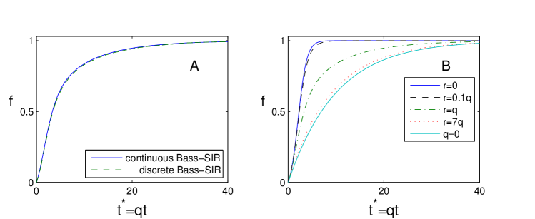
Figure 1: Fraction of adopters in the Bass-SIR model on a nonspatial network, as a function of $t^{*}=qt$. Here $p=0.01$ and $q=0.1$. A) Agreement between the continuous model (2) [solid] and a single simulation of the discrete model (1) with $M=10,000$ [dashes]. Here $r=0.1$. B) The continuous model with $r=0,0.1q,q$, and $7q$. Here $r=0$ is $f_{\rm Bass}$, see (3), and $q=0$ is $f=1-e^{-pt}$.

Cartesian networks.— To analyze the effect of a network with a spatial structure on the diffusion, we first consider periodic $D$-dimensional Cartesian networks, where each node (consumer) is connected to its $2D$ nearest neighbors. In that case, relation (1a) reads

$$\text{Prob}{j~{}\text{adopts in}\choose{(t,t+\Delta t)}}=\left(p+q\frac{i_{j}(t)}{2D}\right)\Delta t+o(\Delta t).$$ (4)

Thus, when $D=1$ the network is a circle and each consumer can be influenced by his left and right neighbors, when $D=2$ the network is a torus and each consumer can be influenced by his up, down, left, and right neighbors, etc.

Our simulations reveal that for given values of $p$, $q$, and $r$, diffusion in a 2D network is faster than in a 1D network but slower than in a 3D network, which, in turn, is slower than in a nonspatial network (Fig. 2). Note that this result is not obvious, since as a network gets more connected, the effect of each connection decreases, so that the maximal internal influence remains $q$, see (1a). The differences among the four networks decrease with $r$. This is because a larger $r$ means shorter internal effects, hence a weaker dependence on the network structure.

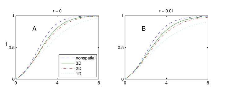
Figure 2: Fraction of adopters in the Bass-SIR model on 1D (dots), 2D (dash-dot), 3D (solid), and nonspatial (dashes) networks. Here $p=0.01$, $q=0.1$, and $M=10,000$. A) $r=0$. B) $r=0.1q$. C) $r=q$. D) $r=7q$.

A priori, it may seem that diffusion becomes faster with $D$, because for a Cartesian network with $M$ consumers, the average distance between consumers decreases as $M^{1/D}$. If diffusion depends on the average distance between consumers, however, then increasing the population size should slow down the fractional adoption, so that $\lim_{M\to\infty}f(t)=0$. This, however, is not the case, since $\lim_{M\to\infty}f\geq 1-e^{-pt}$.

Kolmogorov-Johnson-Mehl-Avrami (KJMA) model.— To understand the effect of the network structure, it is useful to visualize the diffusion process as an on-going random creation of external adopters (“seeds”). Once created, each seed expands through internal adoptions into a cluster of adopters, and expanding clusters can merge into larger clusters. This is nothing but the KJMA model for phase transitions Kolmogorov (1937); Johnson and Mehl (1939); Avrami (1939) from non-adopters to adopters. Unlike its standard applications in physics (but as in algorithmic self-assembly of DNA tiles ), in the Bass-SIR model the evolution of clusters can be more complex, because of the recoveries. To see that, in Fig. 3 we simulate the evolution of single cluster in a 2D network, by placing a single contagious adopter at $t=0$, and setting $p=0$ in (1a) so that all subsequent adoptions are purely-internal. When $r$ is sufficiently small, clusters expand as squares/circles, whose radius increases with time (top row). As $r$ increases, the cluster expands more slowly, the fraction of recovered adopters (out of all adopters) increases, and contagious adopters are mostly concentrated near the cluster surface (second raw). As $r$ further increases (third row), some adopters on the cluster boundary recover before they lead to new adoptions. As a result, clusters evolve into irregular shapes. As $r$ further increases (fourth row), the cluster ceases to expand after some time, once all of its adopters became non-contagious.

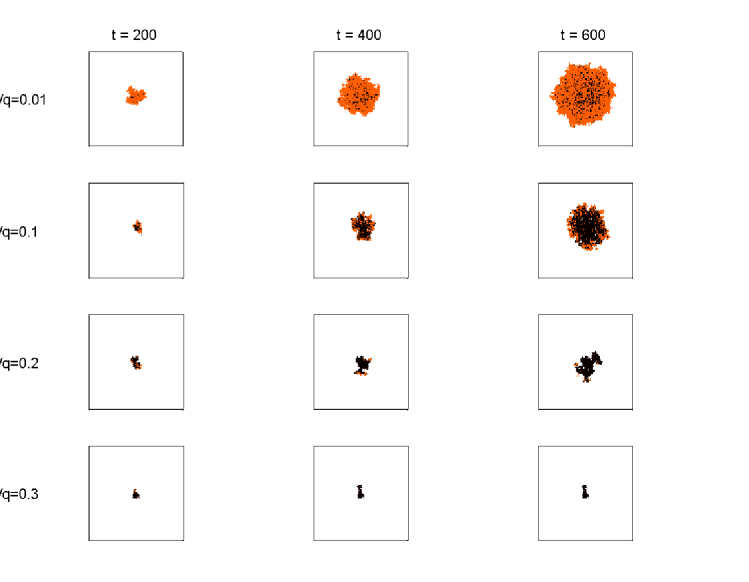
Figure 3: Typical evolution of a single cluster on a 2D network. Here $p=0$, $q=0.1$, and there is a single contagious adopter at $t=0$. Each row corresponds to a different value of $r$. Contagious and recovered adopters are marked by orange and black pixels, respectively.

Since external adoptions are independent of the network structure, the KJMA model implies that the network structure affects the diffusion by affecting the average rate at which clusters expand. We can use this insight to explain the results of Fig. 2, as follows. The average radius $\rho$ of clusters of size $N$ scales as $N^{\frac{1}{D}}$, hence their average surface area (i.e., the number of adopters on the cluster surface which are in direct contact with non-adopters) scales as $\rho^{D-1}\sim N^{\frac{D-1}{D}}$. Therefore, the cluster expansion rate scales as $qN^{\frac{D-1}{D}}/D$, see (4). Hence, the higher $D$ is, the faster the cluster expansion is Fibich and Gibori (2010).

Small-worlds network.— The structure of real-life social networks is different from that of Cartesian networks. Watts and Strogatz Watts and Strogatz (1998) suggested that social networks have a small-worlds structure, whereby most connections are local, but there are also some random long-range connections. They showed that even a small fraction of long-range connections can lead to a dramatic reduction in the average distance between nodes. As a result, epidemics spread much faster on networks with a small-worlds structure.

The acceleration of diffusion by a small-worlds structure should be maximal in the 1D model, because for a given $M$, the average distance is maximal in the 1D model. To induce a “5% small-worlds structure” in the 1D model, we add a link between any two nodes with probability $0.05/M$, so that the average graph degree increases from 2 to 2.05. If, as a result, $j$ is connected to $k_{j}>2$ other consumers, we change the internal effect of each of these consumers on $j$ from $q/2$ to $q/k_{j}$, in accordance with (1a).

Our simulations reveal that the addition of a small-worlds structure has a negligible effect on diffusion of new products (Fig. 4A–C). This is because a small-worlds structure reduces the average distance between agents. This global network property has a negligible effect, however, on diffusion of new products, which depends on the growth rate of a cluster, which, in turn, depends on local properties of the network (such as the grid dimension $D$). Indeed, roughly speaking, if in the absence of a small-worlds structure a certain cluster reaches at time $t$ a size of $N(t)=20$, then adding a “5% small-worlds structure” would increase $N(t)$ at most to $21$.

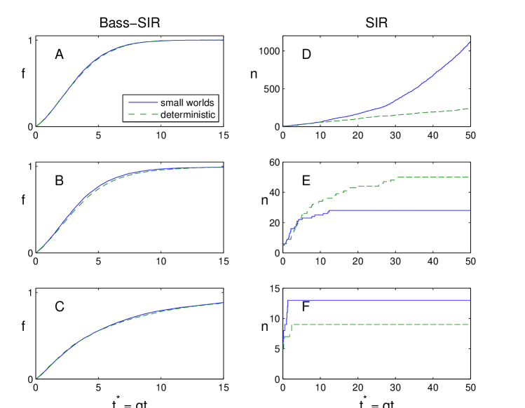
Figure 4: Diffusion on a 1D network with (solid) and without (dashes) a small-worlds structure. Here $q=0.1$ and $M=10,000$. (A)–(C) Fraction of adopters in the discrete Bass-SIR model. Here $p=0.01$, and there are no adopters at $t=0$. A) $r=0$. B) $r=0.1q$. C) $r=q$. (D)–(F) Number of adopters in the discrete SIR model. Here $p=0$, and diffusion starts from 5 randomly-chosen contagious adopters at $t=0$. D) $r=0$. E) $r=0.1q$. F) $r=q$.

To show that our results are not inconsistent with Watts and Strogatz (1998), in Fig. 4D–F we repeat these simulations for the SIR model on the same 1D network with 5% small-worlds structure, and with the same values of $q$ and $r$. Thus, the only differences from Fig. 4A–C is that we now set $p=0$ in (1a), and we let 5 randomly-chosen agents be contagious adopters at $t=0$. In this case the small-worlds structure has a major effect on diffusion, in agreement with Watts and Strogatz (1998). Interestingly, while in the absence of recovery a small-worlds structure always accelerates diffusion, in the presence of recoveries it may also slow it down (Fig. 4E).

Scale-free networks.— Another popular model for social networks is that of a scale-free network. We constructed scale-free networks using the Barabási-Albert (BA) preferential-attachment algorithm Barabási and Albert (1999), in which each new node makes $m$ new links with the existing network nodes, such that the probability of a new node to connect to node $i_{0}$ is $k_{i_{0}}/\sum_{i}k_{i}$, where $k_{i}$ is the degree of node $i$. In the resulting scale-free network, if node $j$ is connected to $k_{j}$ nodes, the effect of each of these nodes on $j$ is ${q}/{k_{j}}$, see (1a).

Our simulations of the discrete Bass-SIR model (1) on scale-free networks show that, as expected, the larger $m$ is, the faster the diffusion (Fig. 5A). Surprisingly, the diffusion on a scale-free network with parameter $m$ is nearly identical to that on a Cartesian network with $D=m$ (Fig. 5B–E). This numerical observation is very surprising, since these networks are different from each other in almost any aspect. Yet, for some reason, the average growth rate of clusters is nearly identical in these networks.

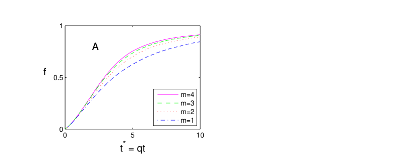
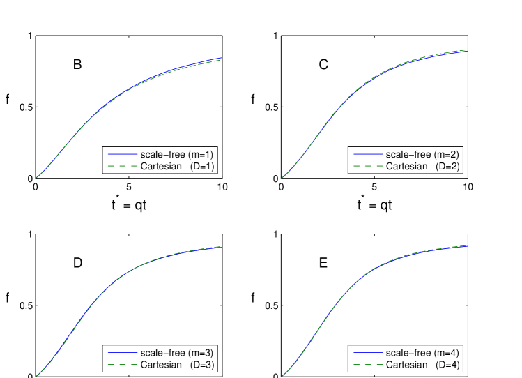
Figure 5: Fraction of adopters in the Bass-SIR model (1) on networks with $p=0.01$, $q=0.1$, $r=0.5q$, and $M=50,000$. A) Scale-free networks with $m=1,2,3$, and $4$. (B)–(E) Scale-free (solid) and Cartesian (dashes) networks. B) $m=D=1$. C) $m=D=2$. D) $m=D=3$. E) $m=D=4$.

Summary.— Two fundamental models of diffusion in social networks are the Bass model for new products, and the SIR model for epidemics Jackson (2008). To the best of our knowledge, these models have not been combined into a single model until now.

The Bass-SIR model is fundamentally different from either of these models. Indeed, since the Bass model does not allow for recovery, it cannot be used for products for which recovery affects the diffusion (e.g., solar PV systems). The SIR model does allow for recovery. However, in the SIR model all external adopters exist at $t=0$, whereas in the Bass-SIR model there is an on-going generation of new external adopters. This difference in the generation of external adopters is not a technical issue, as it leads to a completely different diffusion dynamics.

The key difference between these models is that in the SIR model there is a threshold value of $r$, above which the epidemics will peter out. In contrast, in the Bass-SIR model everyone eventually adopts, since $f(t;p,q,r)\geq f(t;p,0,r)=1-e^{-pt}$ .

The effect of the social network structure in these two models is also very different. Thus, in the SIR model, diffusion occurs through the expansion of a single cluster of internal adopters around “patient zero”. Therefore, the key determinant of diffusion speed is the average distance from patient zero (or more generally, the average distance between individuals), which is a global property of the network. In contrast, diffusion in the Bass-SIR model occurs through the expansion of numerous clusters. Therefore, the diffusion speed is determined by the growth rate of clusters, which depends on local properties of the network. It is because of these differences that, e.g., (i) A small-worlds structure has a large effect on diffusion in the SIR model, but a negligible one in the Bass-SIR model. (ii) Doubling the population size roughly doubles the time $T_{1/2}$ for half of the population to adopt in the SIR model, but has a negligible effect on $T_{1/2}$ in the Bass-SIR model.

The choice between the Bass-SIR model and the SIR model depends on the initiation of the diffusion process. Diseases and rumors that start from a “patent zero” call for the SIR model. External adoptions of new products and external infections from mosquito bites are on-going processes, and thus call for the Bass-SIR model.

Some remaining open questions concern the effect of the network structure.For example, is it true that as $M\to\infty$, the diffusion on a scale-free network becomes identical to that on a Cartesian network with $D=m$? Can we derive macroscopic (averaged) equations for diffusion in Cartesian and scale-free networks? How does recovery affect the phase transition kinetics in the KJMA model?

Acknowledgments.— We thank G. Ariel and O. Raz for useful discussions. This research was conducted while the author was visiting the Center for Scientific Computation and Mathematical Modeling (CSCAMM) at the University of Maryland, and was partially supported by the Kinetic Research Network (KI-Net) under NSF Grant No. RNMS #1107444.

References

- Rogers (2003) E. Rogers, Diffusion of Innovations, 5th ed. (Free Press, New York, 2003).
- Jackson (2008) M. Jackson, Social and Economic Networks (Princeton University Press, Princeton and Oxford, 2008).
- Strang and Soule (1998) D. Strang and S. Soule, Annu. Rev. Sociol. 24, 265 (1998).
- Albert et al. (2000) R. Albert, H. Jeong, and A. Barabási, Nature 406, 378 (2000).
- Pastor-Satorras and Vespignani (2001) R. Pastor-Satorras and A. Vespignani, Phys. Rev. Lett. 86, 3200 (2001).
- Anderson and May (1992) R. Anderson and R. May, Infectious Diseases of Humans (Oxford University Press, Oxford, 1992).
- Mahajan et al. (1993) V. Mahajan, E. Muller, and F. Bass, in Handbooks in Operations Research and Management Science, Vol. 5, edited by J. Eliashberg and G. Lilien (North-Holland, Amsterdam, 1993) pp. 349–408.
- Bass (1969) F. Bass, Management Sci. 15, 215 (1969).
- W.J. Hopp (2004) e. W.J. Hopp, Management Sci. 50, 1763 (2004).
- Graziano and Gillingham (2015) M. Graziano and K. Gillingham, J. Econ. Geogr. 15, 815 (2015).
- Kermack and McKendrick (1927) W. Kermack and A. McKendrick, Proc. Roy. Soc. Lond. A 115, 700 (1927).
- Winfree et al. (1998) E. Winfree, F. Liu, L. Wenzler, and N. Seeman, Nature 394, 539 (1998).
- Fibich and Gibori (2010) G. Fibich and R. Gibori, Oper. Res. 58, 1450 (2010).
- Kolmogorov (1937) A. Kolmogorov, Izv. Akad. Nauk SSSR Ser. Fiz. 1, 335 (1937).
- Johnson and Mehl (1939) W. Johnson and P. Mehl, Trans. Am. Inst. Min. Engin. 135, 416 (1939).
- Avrami (1939) M. Avrami, J. Chem. Phys. 7, 1103 (1939).
- Watts and Strogatz (1998) D. Watts and S. Strogatz, Nature 393, 440 (1998).
- Barabási and Albert (1999) A. Barabási and R. Albert, Science 286, 509 (1999).
- Niu (2002) S. Niu, Math. Problems Engrg. 8, 249 (2002).
- Barish et al. (2009) R. Barish, R. Schulman, P. Rothemund, and E. Winfree, Proc. Natl. Acad. Sci. U.S.A. 106, 6054 (2009).