Interpolative Butterfly Factorization

Abstract

This paper introduces the interpolative butterfly factorization for nearly optimal implementation of several transforms in harmonic analysis, when their explicit formulas satisfy certain analytic properties and the matrix representations of these transforms satisfy a complementary low-rank property. A preliminary interpolative butterfly factorization is constructed based on interpolative low-rank approximations of the complementary low-rank matrix. A novel sweeping matrix compression technique further compresses the preliminary interpolative butterfly factorization via a sequence of structure-preserving low-rank approximations. The sweeping procedure propagates the low-rank property among neighboring matrix factors to compress dense submatrices in the preliminary butterfly factorization to obtain an optimal one in the butterfly scheme. For an $N\times N$ matrix, it takes $O(N\log N)$ operations and complexity to construct the factorization as a product of $O(\log N)$ sparse matrices, each with $O(N)$ nonzero entries. Hence, it can be applied rapidly in $O(N\log N)$ operations. Numerical results are provided to demonstrate the effectiveness of this algorithm.

Keywords. Data-sparse matrix, butterfly algorithm, randomized algorithm, matrix factorization, operator compression, nonuniform Fourier transform, Fourier integral operators.

AMS subject classifications: 44A55, 65R10 and 65T50.

1 Introduction

One key problem in computational harmonic analysis is the rapid evaluation of various transforms to make large-scale scientific computation feasible. These transforms are essentially matrix-vector multiplications, $u=Kg$, where the kernel matrix $K$ is the discrete representation of a transform and the vector $g$ is the discrete representation of a function to be transformed. Inspired by the idea of the butterfly algorithm initially proposed in [24] and later extended in [25], the recently proposed butterfly factorization [20, 21] factorizes a complementary low-rank matrix $K$ of size $N\times N$ into a product of $O(\log N)$ sparse matrices, each with $O(N)$ nonzero entries. After factorization, the application of $K$ has nearly optimal operation and memory complexity of order $N\log N$. Since a wide range of transforms in harmonic analysis admits a matrix representation satisfying the complementary low-rank property [7, 10, 22, 33, 25, 28], the butterfly factorization, once constructed, is a nearly optimal fast algorithm to evaluate these transforms. However, the construction of the butterfly factorization requires $O(N^{2})$ operations in [25] and requires $O(N^{1.5})$ operations in [20, 21], which might still be too expensive in real applications. This paper introduces the interpolative butterfly factorization to construct the factorization in $O(N\log N)$ operation and memory complexity, if the continuous kernel ${K}$ is explicitly available. The interpolative butterfly factorization is a combination of the butterfly algorithm in [7] and a novel structure-preserving matrix compression technique. Hence, the proposed method can be considered as an optimized sparse matrix representation of the butterfly algorithm in [7] with a smaller prefactor in the operation complexity.

Another key problem in modern large-scale computation is the parallel scalability of fast algorithms. Although there have been various fast algorithms like the (nonuniform) fast Fourier transform (FFT) [1, 14, 15], the FFT in polar and spherical coordinates [19, 29, 31, 33], the parallel scalability of some of these traditional algorithms might be still limited in high performance computing. This motivates much effort to improve their parallel scalability [2, 26, 30, 37]. For the same purpose, the interpolative butterfly factorization is proposed as a general framework for highly parallel scalable implementation of a wide range of transforms in harmonic analysis. Since the construction of the butterfly factorization is just a few essentially independent low-rank approximations and the application is a sequence of small matrix-vector multiplications, the butterfly factorization framework significantly reduces communication if implemented in parallel computation.

To be more specific, the interpolative butterfly factorization is proposed for the rapid application of integral transforms of the form

$$u(x)=\int_{\mathbb{R}^{d}}a(x,\xi)e^{2\pi\i\Phi(x,\xi)}g(\xi)d\xi,$$ (1)

where $d$ is the dimension, and ${K}(x,\xi)=a(x,\xi)e^{2\pi\i\Phi(x,\xi)}$ is the kernel function that satisfies following properties:

Assumption 1.1.

Smoothness properties

• $a(x,\xi)$ is an amplitude function that is smooth both in $x$ and $\xi$;

• $\Phi(x,\xi)$ is a phase function that is real analytic for $x$ and $\xi$ and obeys the homogeneity condition of degree $1$ in $\xi$, namely, $\Phi(x,\lambda\xi)=\lambda\Phi(x,\xi)$ for $\lambda>0$.

This transform is also known as the Fourier integral operator (FIO). FIOs are a wide class of operators in harmonic analysis including the (nonuniform) Fourier transform, pseudo-differential operators, and the generalized Radon transform. All these are popular tools in computational physics and chemistry [11, 17, 27, 32, 35], imaging science [6, 8, 23, 38]. For higher dimensional FIOs, the phase function might not be smooth when $\xi=0$. Fortunately, the interpolative butterfly factorization can be adapted to this case following the idea in the multiscale butterfly algorithm in [22].

In most examples, since $a(x,\xi)$ is a smooth symbol of order zero and type $(1,0)$ [3, 5, 9, 34], $a(x,\xi)$ is numerically low-rank in the joint $X$ and $\Omega$ domain and its numerical treatment is relatively easy. Therefore, we will simplify the problem by assuming $a(x,\xi)=1$ in the following discussion.

In a typical setting, it is often assumed that the function $g(\xi)$ decays sufficiently fast so that one can embed the problem in a sufficiently large periodic cell. Without loss of generality, a simple discretization considers functions given on a Cartesian grid

$$X=\left\{x=\left(\frac{n_{1}}{N^{1/d}},\dots,\frac{n_{d}}{N^{1/d}}\right),0\leq n_{1},\dots,n_{d}<N^{1/d}\text{ with }n_{1},\dots,n_{d}\in\mathbb{Z}\right\}$$ (2)

in a unit box in $x$ and defines the discrete integral transform by

$$u(x)=\sum_{\xi\in\Omega}{K}(x,\xi)g(\xi),\quad x\in X,$$ (3)

where

$$\Omega=\left\{\xi=(n_{1},\dots,n_{d}),-\frac{N^{1/d}}{2}\leq n_{1},\dots,n_{d}<\frac{N^{1/d}}{2}\text{ with }n_{1},\dots,n_{d}\in\mathbb{Z}\right\}.$$ (4)

Using the notation in numerical linear algebra, the evaluation of (3) is a matrix-vector multiplication $u=Kg$. Under Assumption 1.1, it can be proved that $K$ is essentially complementary low-rank [7, 22].

1.1 Complementary low-rank matrices and interpolative butterfly factorization

Complementary low-rank matrices have been widely studied in [12, 13, 20, 21, 25, 24, 36]. Let $X$ and $\Omega$ be point sets (not necessary uniformly distributed) in $\mathbb{R}^{d}$ for some dimension $d$. When the kernel $K(x,\xi)$ is discretized on $X\times\Omega$, points in $X$ and $\Omega$ are indexed with row and column indices in the matrix $K$. For simplicity, we also use $X$ and $\Omega$ to denote the sets of row and column indices. Two trees $T_{X}$ and $T_{\Omega}$ of the same depth $L=O(\log N)$, associated with $X$ and $\Omega$ respectively, are constructed by dyadic partitioning. Denote the root level of the tree as level $0$ and the leaf one as level $L$. Such a matrix $K$ of size $O(N)\times O(N)$ is said to satisfy the complementary low-rank property if for any level $\ell$, any node $A$ in $T_{X}$ at level $\ell$, and any node $B$ in $T_{\Omega}$ at level $L-\ell$, the submatrix $K_{A,B}$, obtained by restricting $K$ to the rows indexed by the points in $A$ and the columns indexed by the points in $B$, is numerically low-rank, i.e., for a given precision $\epsilon$ there exists a low-rank approximation of $K_{A,B}$ with an error bounded by $\epsilon$ and the rank bounded polynomially in $\log(1/\epsilon)$ and is independent of $N$. See Figure 1 for an illustration of low-rank submatrices in a complementary low-rank matrix of size $16\times 16$.

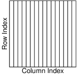
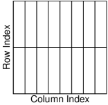
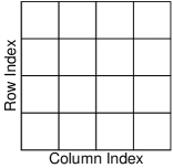
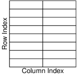
Figure 1: Hierarchical decomposition of the row and column indices of a one-dimensional complementary low-rank matrix of size $16\times 16$. The trees $T_{X}$ ($T_{\Omega}$) has a root containing $16$ column (row) indices and leaves containing a single column (row) index. The rectangles above indicate some of the low-rank submatrices.

It will be shown that, for a complementary low-rank matrix $K$, the matrix-vector multiplication $u=Kg$ can be carried out efficiently via a preliminary interpolative butterfly factorization (IBF) constructed by interpolative low-rank approximations:

$$K\approx U^{L}G^{L-1}\cdots G^{h}M^{h}(H^{h})^{*}\dots(H^{1})^{*}(V^{0})^{*},$$

where the depth $L=O(\log N)$ of $T_{X}$ and $T_{\Omega}$ is assumed to be even, $h=L/2$ is a middle level index, all factors are sparse matrices with $O(N)$ nonzero entries and a large prefactor. Dense blocks in these sparse factors come from interpolative low-rank approximations of low-rank submatrices as illustrated in Figure 1. When the kernel function ${K}$ satisfies Assumption 1.1, each low-rank approximation of these submatrices can be constructed explicitly by Lagrange interpolation with $q$ Chebyshev grid points in each dimension, resulting in dense submatrices of size $q^{d}\times q^{d}$ in sparse factors. Hence, all the matrix factors are available explicitly. However, the low-rank approximation by interpolation is not optimal in the sense that it over estimates the numerical rank $r_{0}$ of the low-rank matrix, i.e. $q^{d}>r_{0}$. Hence, dense blocks in these sparse factors can be further compressed to smaller submatrices of size $r_{0}\times r_{0}$ by a truncated SVD.

The preliminary IBF above can be further compressed by a novel sweeping matrix compression method in two stages. In the sweep-out stage, a sequence of structure-preserving matrix compression is conducted:

$${M^{h}}\approx{C^{h}}{\bar{M}^{h}}{(R^{h})}^{*},$$

$${G^{\ell}}{C^{\ell}}\approx{C^{\ell+1}}{\bar{G}^{\ell}}$$

for $\ell=h,h+1,\dots,L-1$,

$$({H^{\ell}}{R^{\ell}})^{*}\approx({\bar{H}^{\ell}})^{*}({R^{\ell-1}})^{*}$$

for $\ell=h,h-1,\dots,1$, starting from the middle matrix $M^{h}$ and moving towards outer matrices. Let

$${\bar{U}^{L}}={U^{L}}{C^{L}},$$

and

$${\bar{V}^{0}}={V^{0}}{R^{0}},$$

then we have a further compressed factorization

$$K\approx{\bar{U}^{L}\bar{G}^{L-1}\cdots\bar{G}^{h}\bar{M}^{h}(\bar{H}^{h})^{*}\cdots(\bar{H}^{1})^{*}}(\bar{V}^{0})^{*},$$

where all sparse factors have dense submatrices of size closer to $r_{0}\times r_{0}$. ${\bar{U}^{L}}$ and ${\bar{V}^{0}}$ are block-diagonal matrices and the sizes of diagonal blocks depend on the distribution of points in $X$ and $\Omega$. In the case of nonuniform distribution, there might be diagonal blocks with size smaller than $r_{0}\times r_{0}$ in ${\bar{U}^{L}}$ and ${\bar{V}^{0}}$. This motivates the sweep-in stage that contains another sequence of structure-preserving matrix compression:

$${\bar{U}^{L}}\approx{\dot{U}^{L}}\bar{C}^{L},$$

$${\bar{V}^{0}}\approx{\dot{V}^{0}}\bar{R}^{0},$$

$$\bar{C}^{\ell+1}\bar{G}^{\ell}\approx\dot{G}^{\ell}\bar{C}^{\ell}$$

for $\ell=L-1,L-2,\dots,h$,

$$(\bar{H}^{\ell})^{*}(\bar{R}^{\ell-1})^{*}\approx(\bar{R}^{\ell})^{*}(\dot{H}^{\ell})^{*}$$

for $\ell=1,2,\dots,h$, starting from outer matrices to the middle matrix. Finally, let $\dot{M}^{h}=\bar{C}^{h}\bar{M}^{h}(\bar{R}^{h})^{*}$, and one reaches the optimal IBF

$$K\approx{\dot{U}^{L}\dot{G}^{L-1}\cdots\dot{G}^{h}\dot{M}^{h}(\dot{H}^{h})^{*}\cdots(\dot{H}^{1})^{*}}(\dot{V}^{0})^{*},$$ (5)

where all sparse factors have dense submatrices of nearly optimal size.

The optimal IBF represents $K$ as a product of $L+3$ sparse matrices, where all factors are sparse matrices with $O(N)$ nonzero entries, and the prefactor of $O(N)$ is nearly optimal. Once constructed, the cost of applying $K$ to a given vector $g\in\mathbb{C}^{N}$ is $O(N\log N)$.

1.2 Content

The rest of this paper is organized as follows. Section 2 briefly reviews low-rank factorization techniques and the butterfly algorithm in [7]. Section 3 describes the one-dimensional preliminary interpolative butterfly factorization based on interpolative low-rank factorization. Section 4 introduces a structure-preserving matrix compression technique and a sweeping method to further compress the preliminary IBF into an optimal one. Multidimensional extension to a general case when the phase function has singularity at $\xi=0$ is discussed in Section 5. In Section 6, numerical examples are provided to demonstrate the efficiency of the proposed algorithms. Finally, Section 7 concludes this paper with a short discussion.

2 Preliminary

2.1 Low-rank factorization

This section reviews basic tools for efficient low-rank approximations that are repeatedly used in this paper.

Randomized low-rank approximation

For a matrix $Z\in\mathbb{C}^{m\times n}$, we define a rank-$r$ approximate singular value decomposition (SVD) of $Z$ as

$$Z\approx U_{0}\Sigma_{0}V_{0}^{*},$$

where $U_{0}\in\mathbb{C}^{m\times r}$ is unitary, $\Sigma_{0}\in\mathbb{R}^{r\times r}$ is diagonal, and $V_{0}\in\mathbb{C}^{n\times r}$ is unitary. A straightforward method to obtain the optimal rank-$r$ approximation of $Z$ is to compute its truncated SVD, where $U_{0}$ is the matrix with the first $r$ left singular vectors, $\Sigma_{0}$ is a diagonal matrix with the first $r$ singular values in decreasing order, and $V_{0}$ is the matrix with the first $r$ right singular vectors.

The original truncated SVD of $Z$ takes $O(mn\min(m,n))$ operations. More efficient tools have been proposed by introducing randomness in computing approximate SVDs for numerically low-rank matrices. To name a few, the one in [16] is based on applying the matrix to random vectors while another one in [13, 34] relies on sampling the matrix entries randomly. Throughout this paper, the second one is applied to compute large low-rank approximations because it only takes linear operations with respect to the matrix size. Readers are referred to [13, 34] for detailed implementation.

When an approximate SVD $Z\approx U_{0}\Sigma_{0}V_{0}^{*}$ is ready, it can be rearranged in several equivalent ways. First, one can write

$$Z\approx USV^{*},$$

where

$$U=U_{0}\Sigma_{0}^{1/2},\,S=I\text{ and }V^{*}=\Sigma_{0}^{1/2}V_{0}^{*},$$ (6)

so that the left and right factors inherit similar singular values of the original numerical low-rank matrix. Depending on certain applications, sometimes it is better to write the approximation as

$$Z\approx UV^{*}$$

where

$$U=U_{0}\text{ and }V^{*}=\Sigma_{0}V_{0}^{*},$$ (7)

or

$$U=U_{0}\Sigma_{0}\text{ and }V^{*}=V_{0}^{*}$$ (8)

so that only one factor shares the singular values of $Z$.

Interpolative low-rank approximation

The randomized low-rank approximation is efficient if a kernel matrix is given, while the interpolative low-rank approximation is efficient when the explicit formula of the kernel function $K(x,\xi)=e^{2\pi\i\Phi(x,\xi)}$ is available, because the approximation can be constructed explicitly.

Following the theorems in [7, 22], it can be proved that the kernel function $K(x,\xi)=e^{2\pi\i\Phi(x,\xi)}$ satisfies the complementary low-rank property if it fulfills the properties in Assumption 1.1. We will refresh the key idea here for one-dimensional kernels. Let the set $X$ and $\Omega$ refer to the sets defined in (2) and (4). Let $A$ and $B$ be a box pair in the dyadic trees $T_{X}$ and $T_{\Omega}$ such that their levels satisfy $\ell_{A}+\ell_{B}=L$. Then a low-rank separated representation

$$K(x,\xi)=e^{2\pi\i\Phi(x,\xi)}\approx\sum_{t=1}^{r_{\epsilon}}\alpha^{AB}_{t}(x)\beta^{AB}_{t}(\xi)\quad\text{ for }x\in A,\xi\in B$$

exists and can be constructed via the interpolative low-rank approximation as follows.

Let

$$R^{AB}(x,\xi):=\Phi(x,\xi)-\Phi(c_{A},\xi)-\Phi(x,c_{B})+\Phi(c_{A},c_{B}),$$ (9)

where $c_{A}$ and $c_{B}$ are the centers of $A$ and $B$ respectively, then the kernel can be written as

$$e^{2\pi\i\Phi(x,\xi)}=e^{2\pi\i\Phi(c_{A},\xi)}e^{2\pi\i\Phi(x,c_{B})}e^{-2\pi\i\Phi(c_{A},c_{B})}e^{2\pi\i R^{AB}(x,\xi)}.$$ (10)

Hence, the low-rank approximation of $K(x,\xi)$ in $A\times B$ is reduced to the low-rank approximation of $e^{2\pi\i R^{AB}(x,\xi)}$.

Let $w_{A}$ and $w_{B}$ denote the lengths of intervals $A$ and $B$, respectively. A Lagrange interpolation with Chebyshev points in $x$ when $w_{A}\leq 1/\sqrt{N}$ and in $\xi$ when $w_{B}\leq\sqrt{N}$ is applied to construct the low-rank approximation of $e^{2\pi\i R^{AB}(x,\xi)}$. For this purpose, we associate with each interval a Chebyshev grid as follows.

For a fixed integer $r$, the Chebyshev grid of order $r$ on $[-1/2,1/2]$ is defined by

$$\left\{z_{t}=\frac{1}{2}\cos\left(\frac{t\pi}{r-1}\right)\right\}_{0\leq t\leq r-1}.$$

A grid adapted to an interval $A$ with center $c_{A}$ and length $w_{A}$ is then defined via shifting and scaling as

$$\{x_{t}\}_{t=0,1,\ldots,r-1}=\{c_{A}+w_{A}z_{t}\}_{t=0,1,\ldots,r-1}.$$

Given a set of grid points $\{x_{t}\}_{t=0,1,\ldots,r-1}$ in $A$, define Lagrange interpolation polynomials $M^{A}_{t}(x)$ taking value $1$ at $x_{t}$ and $0$ at the other Chebyshev grid points

$$M^{A}_{t}(x)=\prod_{0\leq j\leq r-1,j\neq t}\frac{x-x_{j}}{x_{t}-x_{j}}.$$

Similarly, $M_{t}^{B}$ is denoted as the Lagrange interpolation polynomials for the interval $B$.

Now we are ready to construct the low-rank approximation of $e^{2\pi\i R^{AB}(x,\xi)}$ with $r_{\epsilon}$ Chebyshev points for $\epsilon$-accuracy by interpolation:

• when $w_{B}\leq\sqrt{N}$, the Lagrange interpolation of $e^{2\pi\i R^{AB}(x,\xi)}$ in $\xi$ on a Chebyshev grid $\{g^{B}_{t}\}_{1\leq t\leq r_{\epsilon}}$ adapted to $B$ obeys

  $$e^{2\pi\i R^{AB}(x,\xi)}\approx\sum_{t=1}^{r_{\epsilon}}e^{2\pi\i R^{AB}(x,g^{B}_{t})}M^{B}_{t}(\xi),\quad\forall x\in A,\forall\xi\in B,$$ (11)

• when $w_{A}\leq 1/\sqrt{N}$, the Lagrange interpolation of $e^{2\pi\i R^{AB}(x,\xi)}$ in $x$ on a Chebyshev grid $\{g^{A}_{t}\}_{1\leq t\leq r_{\epsilon}}$ adapted to $A$ obeys

  $$e^{2\pi\i R^{AB}(x,\xi)}\approx\sum_{t=1}^{r_{\epsilon}}M^{A}_{t}(x)e^{2\pi\i R^{AB}(g^{A}_{t},\xi)},\quad\forall x\in A,\forall\xi\in B.$$ (12)

Finally, we are ready to construct the low-rank approximation for the kernel $e^{2\pi\i\Phi(x,\xi)}$:

• when $w_{B}\leq\sqrt{N}$, we multiply (11) with $e^{2\pi\i\Phi(c_{A},\xi)}e^{2\pi\i\Phi(x,c_{B})}e^{-2\pi\i\Phi(c_{A},c_{B})}$, which gives that $\forall x\in A,\forall\xi\in B$

  $$e^{2\pi\i\Phi(x,\xi)}\approx\sum_{t=1}^{r_{\epsilon}}e^{2\pi\i\Phi(x,g^{B}_{t})}\left(e^{-2\pi\i\Phi(c_{A},g^{B}_{t})}M^{B}_{t}(\xi)e^{2\pi\i\Phi(c_{A},\xi)}\right);$$ (13)

• when $w_{A}\leq 1/\sqrt{N}$, multiply (12) with $e^{2\pi\i\Phi(c_{A},\xi)}e^{2\pi\i\Phi(x,c_{B})}e^{-2\pi\i\Phi(c_{A},c_{B})}$ and obtain that $\forall x\in A,\forall\xi\in B$

  $$e^{2\pi\i\Phi(x,\xi)}\approx\sum_{t=1}^{r_{\epsilon}}\left(e^{2\pi\i\Phi(x,c_{B})}M^{A}_{t}(x)e^{-2\pi\i\Phi(g^{A}_{t},c_{B})}\right)e^{2\pi\i\Phi(g^{A}_{t},\xi)}.$$ (14)

The interpolative low-rank factorization can be constructed on-the-fly from the explicit formulas above, which is the main advantage over randomized low-rank approximations. However, since it relies on the information on a fixed Chebyshev grid, the number of Chebyshev points must be sufficiently large to obtain an accurate approximation, i.e., the $\epsilon$-separation rank $r_{\epsilon}$ might be greater than the true numerical rank with $\epsilon$ accuracy.

2.2 Butterfly algorithm

This section provides a brief description of the overall structure of the butterfly algorithm based on the interpolative low-rank approximation in the previous section. In this section, $X$ and $\Omega$ refer to two general sets of $N$ points in $\mathbb{R}$, respectively. With no loss of generality, we assume the points in these two sets are distributed quasi-uniformly but they are not necessarily the sets defined in (2) and (4).

Given an input $\{g(\xi),\xi\in\Omega\}$, the goal is to compute the potentials $\{u(x),x\in X\}$ defined by

$$u(x)=\sum_{\xi\in\Omega}K(x,\xi)g(\xi),\quad x\in X,$$

where $K(x,\xi)$ is a kernel function. The main data structure of the butterfly algorithm is a pair of dyadic trees $T_{X}$ and $T_{\Omega}$. Recall that for any pair of intervals $A\times B\in T_{X}\times T_{\Omega}$ obeying the condition $\ell_{A}+\ell_{B}=L$, the submatrix $\{K(x,\xi)\}_{x\in A,\xi\in B}$ is approximately of a constant rank. An explicit method to construct its low-rank approximation is given by the interpolative low-rank approximation. More precisely, for any $\epsilon>0$, there exists a constant $r_{\epsilon}$ independent of $N$ and two sets of functions $\{\alpha^{AB}_{t}(x)\}_{1\leq t\leq r_{\epsilon}}$ and $\{\beta^{AB}_{t}(\xi)\}_{1\leq t\leq r_{\epsilon}}$ given in (13) or (14) such that

$$\left|K(x,\xi)-\sum_{t=1}^{r_{\epsilon}}\alpha^{AB}_{t}(x)\beta^{AB}_{t}(\xi)\right|\leq\epsilon,\quad\forall x\in A,\forall\xi\in B.$$ (15)

For a given interval $B$ in $\Omega$, define $u^{B}(x)$ to be the restricted potential over the sources $\xi\in B$

$$u^{B}(x)=\sum_{\xi\in B}K(x,\xi)g(\xi).$$

The low-rank property gives a compact expansion for $\{u^{B}(x)\}_{x\in A}$ as summing (15) over $\xi\in B$ with coefficients $g(\xi)$ gives

$$\left|u^{B}(x)-\sum_{t=1}^{r_{\epsilon}}\alpha^{AB}_{t}(x)\left(\sum_{\xi\in B}\beta^{AB}_{t}(\xi)g(\xi)\right)\right|\leq\left(\sum_{\xi\in B}|g(\xi)|\right)\epsilon,\quad\forall x\in A.$$

Therefore, if one can find coefficients $\{\lambda^{AB}_{t}\}_{1\leq t\leq r_{\epsilon}}$ obeying

$$\lambda^{AB}_{t}\approx\sum_{\xi\in B}\beta^{AB}_{t}(\xi)g(\xi),\quad 1\leq t\leq r_{\epsilon},$$ (16)

then the restricted potential $\{u^{B}(x)\}_{x\in A}$ admits a compact expansion

$$\left|u^{B}(x)-\sum_{t=1}^{r_{\epsilon}}\alpha^{AB}_{t}(x)\lambda^{AB}_{t}\right|\leq\left(\sum_{\xi\in B}|g(\xi)|\right)\epsilon,\quad\forall x\in A.$$

The butterfly algorithm below provides an efficient way for computing $\{\lambda^{AB}_{t}\}_{1\leq t\leq r_{\epsilon}}$ recursively. The general structure of the algorithm consists of a top-down traversal of $T_{X}$ and a bottom-up traversal of $T_{\Omega}$, carried out simultaneously. A schematic illustration of the data flow in this algorithm is provided in Figure 2.

Algorithm 2.1.

Butterfly algorithm

1. Preliminaries. Construct the trees $T_{X}$ and $T_{\Omega}$.

2. Initialization. Let $A$ be the root of $T_{X}$. For each leaf interval $B$ of $T_{\Omega}$, construct the expansion coefficients $\{\lambda^{AB}_{t}\}_{1\leq t\leq r_{\epsilon}}$ for the potential $\{u^{B}(x)\}_{x\in A}$ by simply setting

   $$\lambda^{AB}_{t}=\sum_{\xi\in B}\beta^{AB}_{t}(\xi)g(\xi),\quad 1\leq t\leq r_{\epsilon}.$$ (17)

   By the interpolative low-rank approximation, we can define the expansion coefficients $\{\lambda^{AB}_{t}\}_{1\leq t\leq r_{\epsilon}}$ by

   $$\lambda^{AB}_{t}:=e^{-2\pi\i\Phi(c_{A},g_{t}^{B})}\sum_{\xi\in B}\left(M_{t}^{B}(\xi)e^{2\pi\i\Phi(c_{A},\xi)}g(\xi)\right).$$ (18)

3. Recursion. For $\ell=1,2,\ldots,L/2$, visit level $\ell$ in $T_{X}$ and level $L-\ell$ in $T_{\Omega}$. For each pair $(A,B)$ with $\ell_{A}=\ell$ and $\ell_{B}=L-\ell$, construct the expansion coefficients $\{\lambda^{AB}_{t}\}_{1\leq t\leq r_{\epsilon}}$ for the potential $\{u^{B}(x)\}_{x\in A}$ using the low-rank representation constructed at the previous level. Let $P$ be $A$’s parent and $C$ be a child of $B$. Throughout, we shall use the notation $C\succ B$ when $C$ is a child of $B$. At level $\ell-1$, the expansion coefficients $\{\lambda^{PC}_{s}\}_{1\leq s\leq r_{\epsilon}}$ of $\{u^{C}(x)\}_{x\in P}$ are readily available and we have

   $$\left|u^{C}(x)-\sum_{s=1}^{r_{\epsilon}}\alpha^{PC}_{s}(x)\lambda^{PC}_{s}\right|\leq\left(\sum_{\xi\in C}|g(\xi)|\right)\epsilon,\quad\forall x\in P.$$

   Since $u^{B}(x)=\sum_{C\succ B}u^{C}(x)$, the previous inequality implies that

   $$\left|u^{B}(x)-\sum_{C\succ B}\sum_{s=1}^{r_{\epsilon}}\alpha^{PC}_{s}(x)\lambda^{PC}_{s}\right|\leq\left(\sum_{\xi\in B}|g(\xi)|\right)\epsilon,\quad\forall x\in P.$$

   Since $A\subset P$, the above approximation is of course true for any $x\in A$. However, since $\ell_{A}+\ell_{B}=L$, the sequence of restricted potentials $\{u^{B}(x)\}_{x\in A}$ also has a low-rank approximation of size $r_{\epsilon}$, namely,

   $$\left|u^{B}(x)-\sum_{t=1}^{r_{\epsilon}}\alpha^{AB}_{t}(x)\lambda^{AB}_{t}\right|\leq\left(\sum_{\xi\in B}|g(\xi)|\right)\epsilon,\quad\forall x\in A.$$

   Combining the last two approximations, we obtain that $\{\lambda^{AB}_{t}\}_{1\leq t\leq r_{\epsilon}}$ should obey

   $$\sum_{t=1}^{r_{\epsilon}}\alpha^{AB}_{t}(x)\lambda^{AB}_{t}\approx\sum_{C\succ B}\sum_{s=1}^{r_{\epsilon}}\alpha^{PC}_{s}(x)\lambda^{PC}_{s},\quad\forall x\in A.$$ (19)

   This is an over-determined linear system for $\{\lambda^{AB}_{t}\}_{1\leq t\leq r_{\epsilon}}$ when $\{\lambda^{PC}_{s}\}_{1\leq s\leq r_{\epsilon},C\succ B}$ are available. The butterfly algorithm uses an efficient linear transformation approximately mapping $\{\lambda^{PC}_{s}\}_{1\leq s\leq r_{\epsilon},C\succ B}$ into $\{\lambda^{AB}_{t}\}_{1\leq t\leq r_{\epsilon}}$ as follows

   $$\lambda^{AB}_{t}:=e^{-2\pi\i\Phi(c_{A},g_{t}^{B})}\sum_{C\succ B}\sum_{s=1}^{r_{\epsilon}}M_{t}^{B}(g_{s}^{C})e^{2\pi\i\Phi(c_{A},g_{s}^{C})}\lambda^{PC}_{s}.$$ (20)

4. Switch. For the levels visited, the Chebyshev interpolation is applied in variable $\xi$, while the interpolation is applied in variable $x$ for levels $\ell>L/2$. Hence, we are switching the interpolation method at this step. Now we are still working on level $\ell=L/2$ and the same domain pairs $(A,B)$ in the last step. Let $\lambda^{AB}_{s}$ denote the expansion coefficients obtained by Chebyshev interpolation in variable $\xi$ in the last step. Correspondingly, $\{g_{s}^{B}\}_{s}$ are the grid points in $B$ in the last step. We take advantage of the interpolation in variable $x$ in $A$ and generate grid points $\{g_{t}^{A}\}_{1\leq t\leq r_{\epsilon}}$ in $A$. Then we can define new expansion coefficients

   $$\lambda^{AB}_{t}:=\sum_{s=1}^{r_{\epsilon}}e^{2\pi\i\Phi(g_{t}^{A},g_{s}^{B})}\lambda^{AB}_{s}.$$

5. Recursion. Similar to the discussion in Step $3$, we go up in tree $T_{\Omega}$ and down in tree $T_{X}$ at the same time until we reach the level $\ell=L$. We construct the approximation functions by Chebyshev interpolation in variable $x$ as follows:

   $$\alpha_{t}^{AB}(x)=e^{2\pi\i\Phi(x,c_{B})}M_{t}^{A}(x)e^{-2\pi\i\Phi(g_{t}^{A},c_{B})}, \beta_{t}^{AB}(\xi)=e^{2\pi\i\Phi(g_{t}^{A},\xi)}.$$ (21)

   Hence, the new expansion coefficients $\{\lambda^{AB}_{t}\}_{1\leq t\leq r_{\epsilon}}$ can be defined as

   $$\lambda^{AB}_{t}:=\sum_{C\succ B}e^{2\pi\i\Phi(g_{t}^{A},c_{C})}\sum_{s=1}^{r_{\epsilon}}\left(M_{s}^{P}(g_{t}^{A})e^{-2\pi\i\Phi(g_{s}^{P},c_{C})}\lambda^{PC}_{s}\right),$$ (22)

   where again $P$ is $A$’s parent and $C$ is a child interval of $B$.

6. Termination. Finally, $\ell=L$ and set $B$ to be the root node of $T_{\Omega}$. For each leaf interval $A\in T_{X}$, use the constructed expansion coefficients $\{\lambda^{AB}_{t}\}_{1\leq t\leq r_{\epsilon}}$ in (22) to evaluate $u^{B}(x)$ for each $x\in A$,

   $$\begin{split}u(x)=u^{B}(x)&=\sum_{t=1}^{r_{\epsilon}}\alpha^{AB}_{t}(x)\lambda^{AB}_{t}\\ &=e^{2\pi\i\Phi(x,c_{B})}\sum_{t=1}^{r_{\epsilon}}\left(M_{t}^{A}(x)e^{-2\pi\i\Phi(g_{t}^{A},c_{B})}\lambda^{AB}_{t}\right).\end{split}$$ (23)

Figure 2: Trees of the row and column indices. Left: $T_{X}$ for the row indices $X$. Right: $T_{\Omega}$ for the column indices $\Omega$. The interaction between $A\in T_{X}$ and $B\in T_{\Omega}$ starts at the root of $T_{X}$ and the leaves of $T_{\Omega}$.

3 Preliminary interpolative butterfly factorization (IBF)

This section presents the preliminary interpolative butterfly factorization (IBF) for a matrix $K\in\mathbb{C}^{N\times N}$ when its kernel function satisfies Assumption 1.1. In fact, the preliminary interpolative butterfly factorization is a matrix representation of the butterfly algorithm [7]. Similar to the butterfly algorithm, we adopt the same notation of point sets $X$ and $\Omega$, trees $T_{X}$ and $T_{\Omega}$ of depth $L$ (assumed to be an even number). At each level $\ell$, $\ell=0,\dots,L$, we denote the $i$th node at level $\ell$ in $T_{X}$ as $A^{\ell}_{i}$ for $i=0,1,\dots,2^{\ell}-1$ and the $j$th node at level $L-\ell$ in $T_{\Omega}$ as $B^{L-\ell}_{j}$ for $j=0,1,\dots,2^{L-\ell}-1$. These nodes naturally partition $K$ into $O(N)$ submatrices $K_{A^{\ell}_{i},B^{L-\ell}_{j}}$. For simplicity, we write $K^{\ell}_{i,j}:=K_{A^{\ell}_{i},B^{L-\ell}_{j}}$, where the superscript is used to indicate the level (in $T_{X}$). With abuse of notation, sometimes we use the subscripts ${i,j}$ and the superscript $\ell$ on a matrix or a vector corresponding the domain pair $(A^{\ell}_{i},B^{L-\ell}_{j})$ for simplicity, although it is not a submatrix or a subvector restricted in $(A^{\ell}_{i},B^{L-\ell}_{j})$.

The preliminary IBF is based on the observation that the butterfly algorithm in Section 2.2 can be written in a form of matrix factorization. The operations in Step 2 to 6 in Algorithm 2.1 are essentially a sequence of matrix vector multiplications with $O(\log N)$ multiplications, each matrix of which has only $O(r_{\epsilon}^{2}N)$ nonzero entries. Since all the operations are given explicitly based on Chebyshev interpolation, these sparse matrices can be formed by explicit formulas. By formulating these matrices step by step following the flow in Algorithm 2.1, the preliminary IBF is proposed as follows.

1. Preliminaries. Construct the trees $T_{X}$ and $T_{\Omega}$.

2. Initialization. At level $\ell=0$, for each $j=0,1,\dots,2^{L}-1$, let $A$ be $\Omega$ and $B$ be $B^{L}_{j}$ of $T_{\Omega}$. Construct the expansion coefficients $\{\lambda^{AB}_{t}\}_{1\leq t\leq r_{\epsilon}}$ for the potential $\{u^{B}(x)\}_{x\in A}$ by simply setting

   $$\lambda^{AB}_{t}:=e^{-2\pi\i\Phi(c_{A},g_{t}^{B})}\sum_{\xi\in B}\left(M_{t}^{B}(\xi)e^{2\pi\i\Phi(c_{A},\xi)}g(\xi)\right).$$ (24)

   For each $j=0,1,\dots,2^{L}-1$, a column vector $\Lambda^{0}_{j}$ corresponding to the domain pair $(A,B)=(\Omega,B^{L}_{j})$ is defined as

   $$\Lambda^{0}_{j}=\begin{pmatrix}\lambda^{AB}_{1}\\ \vdots\\ \lambda^{AB}_{r_{\epsilon}}\end{pmatrix}.$$

   Let $(V^{0}_{j})^{*}\in\mathbb{C}^{r_{\epsilon}\times O(1)}$ represent the linear transformation in (24) and $g^{0}_{j}$ be the vector representing $g(\xi)$ for $\xi\in B^{L}_{j}$. Then we have

   $$\Lambda^{0}_{j}=(V^{0}_{j})^{*}g^{0}_{j}.$$ (25)

   As we shall see later, the conjugate transpose ^∗ is applied for the purpose of notation consistency. By assembling the matrix-vector multiplications in (25), all the operations in this step can be written as

   $$\Lambda^{0}=\begin{pmatrix}\Lambda^{0}_{0}\\ \vdots\\ \Lambda^{0}_{2^{L}-1}\end{pmatrix}=(V^{0})^{*}g,$$

   where

   $$V^{0}=\text{ diag}\left\{V^{0}_{0},V^{0}_{1},\cdots,V^{0}_{2^{L}-1}\right\}.$$

3. Recursion. For $\ell=1,2,\ldots,L/2$, visit level $\ell$ in $T_{X}$ and level $L-\ell$ in $T_{\Omega}$. At each level $\ell$, for each pair $(A,B)$ with $\ell_{A}=\ell$ and $\ell_{B}=L-\ell$, construct the expansion coefficients $\{\lambda^{AB}_{t}\}_{1\leq t\leq r_{\epsilon}}$ using the low-rank representation constructed at the previous level ($\ell=0$ is the initialization step). Let $P$ be $A$’s parent and $C$ be a child of $B$. An efficient linear transformation approximately mapping $\{\lambda^{PC}_{s}\}_{1\leq s\leq r_{\epsilon},C\succ B}$ into $\{\lambda^{AB}_{t}\}_{1\leq t\leq r_{\epsilon}}$ is constructed by

   $$\lambda^{AB}_{t}:=e^{-2\pi\i\Phi(c_{A},g_{t}^{B})}\sum_{C\succ B}\sum_{s=1}^{r_{\epsilon}}M_{t}^{B}(g_{s}^{C})e^{2\pi\i\Phi(c_{A},g_{s}^{C})}\lambda^{PC}_{s}.$$ (26)

   At each level $\ell$, for each $i=0,1,\dots,2^{\ell}-1$ and $j=0,1,\dots,2^{L-\ell}-1$, a column vector $\Lambda^{\ell}_{i,j}$ is defined as

   $$\Lambda^{\ell}_{i,j}=\begin{pmatrix}\lambda^{AB}_{1}\\ \vdots\\ \lambda^{AB}_{r_{\epsilon}}\end{pmatrix}\in\mathbb{C}^{r_{\epsilon}},$$ (27)

   where the domain pair $(A,B)=(A^{\ell}_{i},B^{L-\ell}_{j})$. For a fixed $j$, stacking vectors $\{\Lambda^{\ell}_{i,j}\}_{i}$ together forms a larger column vector $\Lambda^{\ell}_{j}$ and stacking vectors $\{\Lambda^{\ell}_{j}\}_{j}$ together forms a column vector $\Lambda^{\ell}$,

   $$\Lambda^{\ell}_{j}=\begin{pmatrix}\Lambda^{\ell}_{0,j}\\ \vdots\\ \Lambda^{\ell}_{2^{\ell}-1,j}\end{pmatrix},\quad\Lambda^{\ell}=\begin{pmatrix}\Lambda^{\ell}_{0}\\ \vdots\\ \Lambda^{\ell}_{2^{L-\ell}-1}\end{pmatrix}.$$

   The linear transformation in (26) maps two small column vectors $\Lambda^{\ell-1}_{i,2j}$ and $\Lambda^{\ell-1}_{i,2j+1}$ at the previous level $\ell-1$ to a small column vector $\Lambda^{\ell}_{2i,j}$ if $A$ is the first child of $P$ (or $\Lambda^{\ell}_{2i+1,j}$ if $A$ is the second child of $P$) at the current level $\ell$ for all $i=0,1,\dots,2^{\ell-1}-1$ and $j=0,1,\dots,2^{L-\ell}-1$. Hence, for each pair $(i,j)$, the linear transformation in (26) can be written as a matrix vector multiplication

   $$\Lambda^{\ell}_{2i,j}=\begin{pmatrix}H^{\ell}_{2i,2j}&H^{\ell}_{2i,2j+1}\end{pmatrix}\begin{pmatrix}\Lambda^{\ell-1}_{i,2j}\\ \Lambda^{\ell-1}_{i,2j+1}\end{pmatrix},$$ (28)

   where $H^{\ell}_{2i,2j}\in\mathbb{C}^{r_{\epsilon}\times r_{\epsilon}}$ and $H^{\ell}_{2i,2j+1}\in\mathbb{C}^{r_{\epsilon}\times r_{\epsilon}}$, or

   $$\Lambda^{\ell}_{2i+1,j}=\begin{pmatrix}H^{\ell}_{2i+1,2j}&H^{\ell}_{2i+1,2j+1}\end{pmatrix}\begin{pmatrix}\Lambda^{\ell-1}_{i,2j}\\ \Lambda^{\ell-1}_{i,2j+1}\end{pmatrix},$$ (29)

   where $H^{\ell}_{2i+1,2j}\in\mathbb{C}^{r_{\epsilon}\times r_{\epsilon}}$ and $H^{\ell}_{2i+1,2j+1}\in\mathbb{C}^{r_{\epsilon}\times r_{\epsilon}}$. Assemble the above small matrices together to get

   $$H^{\ell}_{j}=\begin{pmatrix}H^{\ell}_{0,2j}&H^{\ell}_{1,2j}&&&\\ &&H^{\ell}_{2,2j}&H^{\ell}_{3,2j}&&\\ &&&&\ddots&&\\ &&&&&H^{\ell}_{2^{\ell}-2,2j}&H^{\ell}_{2^{\ell}-1,2j}\\ \hline\cr H^{\ell}_{0,2j+1}&H^{\ell}_{1,2j+1}&&&\\ &&H^{\ell}_{2,2j+1}&H^{\ell}_{3,2j+1}&&\\ &&&&\ddots&\\ &&&&&H^{\ell}_{2^{\ell}-2,2j+1}&H^{\ell}_{2^{\ell}-1,2j+1}\end{pmatrix}$$

   for $j=0,1,\dots,2^{L-\ell}-1$ and

   $$H^{\ell}=\begin{pmatrix}H^{\ell}_{0}&&&\\ &H^{\ell}_{1}&&\\ &&\ddots&\\ &&&H^{\ell}_{2^{L-\ell}-1}\\ \end{pmatrix},$$

   then all the operations in this step can be represented by a large matrix-vector multiplication

   $$\Lambda^{\ell}=(H^{\ell})^{*}\Lambda^{\ell-1}$$

   for $\ell=1,2,\ldots,L/2$.

4. Switch. For the levels visited, the Chebyshev interpolation is applied in variable $\xi$, while the interpolation is applied in variable $x$ for levels $\ell>L/2$. Hence, we are switching the interpolation method at this step. Now we are still working at level $\ell=L/2$ and the same domain pairs $(A,B)=(A^{L/2}_{i},B^{L/2}_{j})$ in the last step. Recall that $\Lambda^{L/2}$ denote the expansion coefficients obtained by Chebyshev interpolation in variable $\xi$ in the last step. Correspondingly, $\{g_{s}^{B}\}_{s}$ are the grid points in $B$ in the last step. We take advantage of the interpolation in variable $x$ in $A$ and generate grid points $\{g_{t}^{A}\}_{1\leq t\leq r_{\epsilon}}$ in $A$. Then we can define new expansion coefficients for Chebyshev interpolation in variable $x$ for future steps as

   $$\lambda^{AB}_{t}:=\sum_{s=1}^{r_{\epsilon}}e^{2\pi\i\Phi(g_{t}^{A},g_{s}^{B})}\lambda^{AB}_{s}.$$ (30)

   Let $\tilde{M}^{L/2}_{i,j}\in\mathbb{C}^{r_{\epsilon}\times r_{\epsilon}}$ represent the linear transformation introduced by $\{e^{2\pi\i\Phi(g_{t}^{A},g_{s}^{B})}\}_{1\leq t\leq r_{\epsilon},1\leq s\leq r_{\epsilon}}$ for $i$, $j=0,1,\cdots,2^{L/2}-1$. Then (30) is equivalent to

   $$\tilde{\Lambda}^{L/2}_{i,j}=\tilde{M}^{L/2}_{i,j}\Lambda^{L/2}_{i,j}$$

   for each domain pair $(A,B)=(A^{L/2}_{i},B^{L/2}_{j})$. Recall that

   $$\Lambda^{L/2}_{j}=\begin{pmatrix}\Lambda^{L/2}_{0,j}\\ \vdots\\ \Lambda^{L/2}_{2^{L/2}-1,j}\end{pmatrix},\text{ and }\Lambda^{L/2}=\begin{pmatrix}\Lambda^{L/2}_{0}\\ \vdots\\ \Lambda^{L/2}_{2^{L/2}-1}\end{pmatrix}.$$

   If we define the expansion coefficients in a new order by

   $$\tilde{\Lambda}^{L/2}_{i}=\begin{pmatrix}\tilde{\Lambda}^{L/2}_{i,0}\\ \vdots\\ \tilde{\Lambda}^{L/2}_{i,2^{L/2}-1}\end{pmatrix},\text{ and }\tilde{\Lambda}^{L/2}=\begin{pmatrix}\tilde{\Lambda}^{L/2}_{0}\\ \vdots\\ \tilde{\Lambda}^{L/2}_{2^{L/2}-1}\end{pmatrix},$$

   then all the operations in (30) for all domain pairs can be represented by a large matrix-vector multiplication

   $$\tilde{\Lambda}^{L/2}=M^{L/2}\Lambda^{L/2},$$

   where

   $$M^{L/2}=\begin{pmatrix}M^{L/2}_{0,0}&M^{L/2}_{0,1}&\cdots&M^{L/2}_{0,2^{L/2}-1}\\ M^{L/2}_{1,0}&M^{L/2}_{1,1}&&M^{L/2}_{1,2^{L/2}-1}\\ \vdots&&\ddots&\\ M^{L/2}_{2^{L/2}-1,0}&M^{L/2}_{2^{L/2}-1,1}&&M^{L/2}_{2^{L/2}-1,2^{L/2}-1}\end{pmatrix}\in\mathbb{C}^{r_{\epsilon}N\times r_{\epsilon}N}$$

   and $M^{L/2}_{i,j}\in\mathbb{C}^{r_{\epsilon}\sqrt{N}\times r_{\epsilon}\sqrt{N}}$ is also a $2^{L/2}\times 2^{L/2}$ block matrix with the only nonzero block at the location $(j,i)$ being $\tilde{M}^{L/2}_{i,j}\in\mathbb{C}^{r_{\epsilon}\times r_{\epsilon}}$. By the abuse of notation, we drop the tilde notation $\tilde{\cdot}$ of the expansion coefficients in the second half of the algorithm description.

5. Recursion. Similar to the discussion in Step $3$, we go up in tree $T_{\Omega}$ and down in tree $T_{X}$ at the same time for all level $\ell=L/2+1,\cdots,L$. At each level $\ell$, for any domain pair $(A,B)=(A^{\ell}_{i},B^{L-\ell}_{j})$, for $i=0,1,\dots,2^{\ell}-1$ and $j=0,1,\dots,2^{L-\ell}-1$, we construct the new expansion coefficients $\{\lambda^{AB}_{t}\}_{1\leq t\leq r_{\epsilon}}$ by

   $$\lambda^{AB}_{t}:=\sum_{C\succ B}e^{2\pi\i\Phi(g_{t}^{A},c_{C})}\sum_{s=1}^{r_{\epsilon}}\left(M_{s}^{P}(g_{t}^{A})e^{-2\pi\i\Phi(g_{s}^{P},c_{C})}\lambda^{PC}_{s}\right),$$ (31)

   where again $P$ is $A$’s parent and $C$ is a child interval of $B$. The coefficients are assembled as

   $$\Lambda^{\ell}_{i,j}=\begin{pmatrix}\lambda^{AB}_{1}\\ \vdots\\ \lambda^{AB}_{r_{\epsilon}}\end{pmatrix},\quad\Lambda^{\ell}_{i}=\begin{pmatrix}\Lambda^{\ell}_{i,0}\\ \vdots\\ \Lambda^{\ell}_{i,2^{L-\ell}-1}\end{pmatrix},\text{ and }\Lambda^{\ell}=\begin{pmatrix}\Lambda^{\ell}_{0}\\ \vdots\\ \Lambda^{\ell}_{2^{\ell}-1}\end{pmatrix},$$

   for $i=0,1,\dots,2^{\ell}-1$, $j=0,1,\dots,2^{L-\ell}-1$.

   Similarly to the first recursion step, the linear transformation in (31) maps two small column vectors $\Lambda^{\ell-1}_{i,2j}$ and $\Lambda^{\ell-1}_{i,2j+1}$ at the previous level $\ell-1$ to a small column vector $\Lambda^{\ell}_{2i,j}$ if $A$ is the first child of $P$ (or $\Lambda^{\ell}_{2i+1,j}$ if $A$ is the second child of $P$) at the current level $\ell$ for all $i=0,1,\dots,2^{\ell-1}-1$ and $j=0,1,\dots,2^{L-\ell}-1$. Hence, for each pair $(i,j)$, the linear transformation in (31) can be written as a matrix vector multiplication

   $$\Lambda^{\ell}_{2i,j}=\begin{pmatrix}G^{\ell-1}_{2i,2j}&G^{\ell-1}_{2i,2j+1}\end{pmatrix}\begin{pmatrix}\Lambda^{\ell-1}_{i,2j}\\ \Lambda^{\ell-1}_{i,2j+1}\end{pmatrix},$$ (32)

   where $G^{\ell-1}_{2i,2j}\in\mathbb{C}^{r_{\epsilon}\times r_{\epsilon}}$ and $G^{\ell-1}_{2i,2j+1}\in\mathbb{C}^{r_{\epsilon}\times r_{\epsilon}}$, or

   $$\Lambda^{\ell}_{2i+1,j}=\begin{pmatrix}G^{\ell-1}_{2i+1,2j}&G^{\ell-1}_{2i+1,2j+1}\end{pmatrix}\begin{pmatrix}\Lambda^{\ell-1}_{i,2j}\\ \Lambda^{\ell-1}_{i,2j+1}\end{pmatrix},$$ (33)

   where $G^{\ell-1}_{2i+1,2j}\in\mathbb{C}^{r_{\epsilon}\times r_{\epsilon}}$ and $G^{\ell-1}_{2i+1,2j+1}\in\mathbb{C}^{r_{\epsilon}\times r_{\epsilon}}$. Assemble the above small matrices together to get

   $$G^{\ell-1}_{i}=\begin{pmatrix}G^{\ell-1}_{2i,0}&G^{\ell-1}_{2i,1}&&&\\ &&G^{\ell-1}_{2i,2}&G^{\ell-1}_{2i,3}&&\\ &&&&\ddots&\\ &&&&&G^{\ell-1}_{2i,2^{L-\ell}-2}&G^{\ell-1}_{2i,2^{L-\ell}-1}\\ \hline\cr G^{\ell-1}_{2i+1,0}&G^{\ell-1}_{2i+1,1}&&&\\ &&G^{\ell-1}_{2i+1,2}&G^{\ell-1}_{2i+1,3}&&\\ &&&&\ddots&\\ &&&&&G^{\ell-1}_{2i+1,2^{L-\ell}-2}&G^{\ell-1}_{2i+1,2^{L-\ell}-1}\end{pmatrix}$$

   for $i=0,1,\dots,2^{\ell-1}-1$ and

   $$G^{\ell-1}=\begin{pmatrix}G^{\ell-1}_{0}&&&\\ &G^{\ell-1}_{1}&&\\ &&\ddots&\\ &&&G^{\ell-1}_{2^{\ell-1}-1}\\ \end{pmatrix},$$

   then all the operations in this step can be represented by a large matrix-vector multiplication

   $$\Lambda^{\ell}=G^{\ell-1}\Lambda^{\ell-1}$$

   for $\ell=L/2+1,\ldots,L$.

6. Termination. Finally, $\ell=L$ again and set $B=\Omega$. For each leaf interval $A=A^{L}_{i}\in T_{X}$, $i=0,1,\dots,2^{L}-1$, use the constructed expansion coefficients $\delta^{L}$ in the last step to evaluate $u^{B}(x)$ for each $x\in A$,

   $$\begin{split}u(x)=u^{B}(x)&=\sum_{t=1}^{r_{\epsilon}}\alpha^{AB}_{t}(x)\lambda^{AB}_{t}\\ &=e^{2\pi\i\Phi(x,c_{B})}\sum_{t=1}^{r_{\epsilon}}\left(M_{t}^{A}(x)e^{-2\pi\i\Phi(g_{t}^{A},c_{B})}\lambda^{AB}_{t}\right).\end{split}$$ (34)

   For each domain pair $(A,B)=(A^{L}_{i},\Omega)$, let $U^{L}_{i}\in\mathbb{C}^{O(1)\times r_{\epsilon}}$ be the matrix representing the linear transformation in (34). Define

   $$U^{L}=\text{ diag}\left\{U^{L}_{0},U^{L}_{1},\cdots,U^{L}_{2^{L}-1}\right\}.$$

   By the same argument in the initialization step, the matrix-vector multiplication format of all the operations in this step is

   $$u=U^{L}\Lambda^{L}.$$

In sum, by the discussion above, $K$ is approximated by the preliminary IBF as

$$K\approx U^{L}G^{L-1}\cdots G^{L/2}M^{L/2}(H^{L/2})^{*}\dots(H^{1})^{*}(V^{0})^{*}.$$

Since the total number of nonzero entries of the above sparse factors is $O(r_{\epsilon}^{2}N\log N)$ and each factors can be constructed explicitly by the Chebyshev interpolation, the operation and memory complexity of constructing and applying the IBF is $O(r_{\epsilon}^{2}N\log N)$.

4 Optimal interpolative butterfly factorization

Recall that at each level $\ell$ the kernel matrix $K$ restricted in a domain pair $(A,B)=(A^{\ell}_{i},B^{L-\ell}_{j})$, denoted as $K^{\ell}_{ij}$, is a numerically low-rank matrix. For a given $\epsilon$, let $r_{0}(\epsilon,\ell,i,j)$ be the numerical rank provided by a truncated SVD of $K^{\ell}_{ij}$. With abuse of notation, let us use $r_{0}$ for simplicity. Similarly, let $r_{\epsilon}$ denote the numerical rank provided by the low-rank approximation by Chebyshev interpolation. Since $r_{\epsilon}$ might not be able to reveal the optimal numerical rank $r_{0}$, i.e. $r_{\epsilon}>r_{0}$. The $O(r_{\epsilon}^{2})$ prefactor in the complexity of the preliminary IBF might be far from the optimal one, $r_{0}^{2}$.

The above observation motivates the design of the novel sweeping matrix compression based on a sequence of structure-preserving matrix compression. The sweeping matrix compression further compresses the preliminary IBF into an optimal one. The main idea is to propagate low-rank property among matrix factors in the preliminary IBF and to shrink the size of dense submatrices in these matrix factors by the randomized low-rank approximation in Section 2.

The structure-preserving matrix compression is introduced in Section 4.1. The sweeping matrix compression consists of two stages, the sweep-out and the sweep-in stages. They will be presented in Section 4.2 and Section 4.3, respectively.

4.1 Structure-preserving matrix compression

One key idea to construct the optimal IBF is the sweeping matrix compression via a sequence of structure-preserving matrix compression introduced below. Suppose $S$ is a block matrix with $m\times k$ blocks, i.e.,

$$S=\begin{pmatrix}S_{0,0}&S_{0,1}&\cdots&S_{0,k-1}\\ S_{1,0}&S_{1,1}&&S_{1,k-1}\\ \vdots&&\ddots&\\ S_{m-1,0}&S_{m-1,1}&&S_{m-1,k-1}\end{pmatrix}\in\mathbb{C}^{mr\times kr}.$$

For simplicity, we assume that each block in $S$ is of size $r\times r$. The structure-preserving matrix compression can be easily extended to block matrices with different block sizes. Let $D$ be a block-diagonal matrix with $k$ diagonal blocks and each diagonal block is of size $r\times r_{0}$ with $r_{0}<r$, i.e.,

$$D=\begin{pmatrix}D_{0}&&&\\ &D_{1}&&\\ &&\ddots&\\ &&&D_{k-1}\end{pmatrix}\in\mathbb{C}^{kr\times kr_{0}}.$$

Let $P$ be the product of $S$ and $D$, i.e.,

$$P=\begin{pmatrix}P_{0,0}&P_{0,1}&\cdots&P_{0,k-1}\\ P_{1,0}&P_{1,1}&&P_{1,k-1}\\ \vdots&&\ddots&\\ P_{m-1,0}&P_{m-1,1}&&P_{m-1,k-1}\end{pmatrix}=\begin{pmatrix}S_{0,0}D_{0}&S_{0,1}D_{1}&\cdots&S_{0,k-1}D_{k-1}\\ S_{1,0}D_{0}&S_{1,1}D_{1}&&S_{1,k-1}D_{k-1}\\ \vdots&&\ddots&\\ S_{m-1,0}D_{0}&S_{m-1,1}D_{1}&&S_{m-1,k-1}D_{k-1}\end{pmatrix}\in\mathbb{C}^{mr\times kr_{0}}.$$

We call that the matrix pencil $(S,D)$ has the structure-preserving low rank property of type $(m,k,r,r_{0})$, if it satisfies the following condition. For each $i=1$, $\dots$, $m$, there exists a low-rank approximation

$$\begin{pmatrix}P_{i,0}&P_{i,1}&\cdots&P_{i,k-1}\end{pmatrix}\approx\tilde{D}_{i}\begin{pmatrix}\tilde{S}_{i,0}&\tilde{S}_{i,1}&\cdots&\tilde{S}_{i,k-1}\end{pmatrix}$$ (35)

where $\tilde{D}_{i}\in\mathbb{C}^{r\times r_{0}}$ and $\tilde{S}_{i,j}\in\mathbb{C}^{r_{0}\times r_{0}}$ for $j=0,1,\dots,k-1$. Under the assumption of the structure-preserving low-rank property of type $(m,k,r,r_{0})$, by assembling the low-rank approximations in (35) into two large factors $\tilde{D}$ and $\tilde{S}$, the structure-preserving matrix compression of type $(m,k,r,r_{0})$ factorizes $SD$ as

$$SD\approx\tilde{D}\tilde{S},$$

where $\tilde{D}$ is again a block-diagonal matrix with $k$ diagonal blocks of size $r\times r_{0}$, $\tilde{S}$ is a block matrix with $m\times k$ blocks of size $r_{0}\times r_{0}$, $S$ and $\tilde{S}$ share the same column indices of nonzero blocks in each row block (see Figure 3 for an example).

= $\approx$

Figure 3: The structure-preserving matrix compression of type $(4,4,4,1)$ $SD=P\approx\tilde{D}\tilde{S}$, where $S\in\mathbb{C}^{16\times 16}$ (left matrix), $P\in\mathbb{C}^{16\times 4}$ (middle matrix), and $\tilde{S}\in\mathbb{C}^{4\times 4}$ (right matrix) are $4\times 4$ block matrices with the same sparsity pattern, $D\in\mathbb{C}^{16\times 4}$ (middle left matrix) and $\tilde{D}\in\mathbb{C}^{16\times 4}$ (middle right matrix) are $4\times 4$ block-diagonal matrices,

4.2 Sweeping matrix compression: sweep-out stage

The optimal IBF of $K$ is built in two stages. In the first stage, we further compress the matrix factors in the preliminary IBF,

$$K\approx U^{L}G^{L-1}\cdots G^{h}{M^{h}}(H^{h})^{*}\dots(H^{1})^{*}(V^{0})^{*},$$

sweeping from the middle matrix $M^{h}$ and moving out towards $U^{L}$ and $V^{0}$. Recall that each nonzero submatrix $\tilde{M}^{h}_{ij}\in\mathbb{C}^{r_{\epsilon}\times r_{\epsilon}}$ in $M^{h}$ is the kernel function $K(x.\xi)$ evaluated at the Chebyshev grid points in the domain pairs $(A,B)=(A^{h}_{i},B^{h}_{j})$ at level $h$. Hence, $\tilde{M}^{h}_{ij}$ is a numerically low-rank matrix if $r_{\epsilon}>r_{0}$ (which is usually the case in existing butterfly algorithms using Chebyshev interpolations to construct low-rank factorizations). Hence, ${M^{h}}$ can be further compressed via a rank-revealing low-rank approximation of each $\tilde{M}^{h}_{ij}$, e.g., the truncated SVD, into

$${M^{h}}\approx{C^{h}}{\bar{M}^{h}}{(R^{h})}^{*},$$

resulting the middle level factorization

$$K\approx U^{L}G^{L-1}\cdots G^{h}{C^{h}}{\bar{M}^{h}}{(R^{h})}^{*}(H^{h})^{*}\dots(H^{1})^{*}(V^{0})^{*}.$$ (36)

The middle level factorization is described in detail in Section 4.2.1.

Next, we recursively factorize

$${G^{\ell}}{C^{\ell}}\approx{C^{\ell+1}}{\bar{G}^{\ell}}$$

for $\ell=h,h+1,\dots,L-1$,

$$({H^{\ell}}{R^{\ell}})^{*}\approx({\bar{H}^{\ell}})^{*}({R^{\ell-1}})^{*}$$

for $\ell=h,h-1,\dots,1$, since the matrix pencils $(G^{\ell},C^{\ell})$ and $(H^{\ell},R^{\ell})$ satisfy the structure-preserving low-rank property. In another word, ${C^{\ell}}$ and ${R^{\ell}}$ propagate the low-rank property of $M^{h}$ to $G^{\ell}$ and $H^{\ell}$, respectively, so that we can further compress $G^{\ell}$ and $H^{\ell}$. After this recursive factorization, let

$${\bar{U}^{L}}={U^{L}}{C^{L}},$$

and

$${\bar{V}^{0}}={V^{0}}{R^{0}},$$

then one reaches at a more compressed IBF of $K$:

$$K\approx\bar{U}^{L}\bar{G}^{L-1}\cdots\bar{G}^{h}\bar{M}^{h}(\bar{H}^{h})^{*}\cdots(\bar{H}^{1})^{*}(\bar{V}^{0})^{*},$$ (37)

where all factors are sparse matrices with almost $O(r_{0}^{2}N)$ nonzero entries. We refer to this stage as the recursive factorization and it is discussed in detail in Section 4.2.2 and 4.2.3.

4.2.1 Middle level factorization

Recall that we denote the $i$th node at level $\ell$ in $T_{X}$ as $A^{\ell}_{i}$ for $i=0,1,\dots,2^{\ell}-1$ and the $j$th node at level $L-\ell$ in $T_{\Omega}$ as $B^{L-\ell}_{j}$ for $j=0,1,\dots,2^{L-\ell}-1$. Let $h=L/2$ and $m=2^{L/2}$. Since the nonzero submatrix $\tilde{M}^{h}_{ij}$ in $M^{h}$ is a matrix representation of the kernel function $K(x,\xi)$ evaluated at the Chebyshev grid points $\{g_{t}^{A}\}_{t}$ and $\{g_{s}^{B}\}_{s}$ for the domain pair $(A,B)=(A^{h}_{i},B^{h}_{j})$ at the middle level $\ell=h$. $\tilde{M}^{h}_{ij}\in\mathbb{C}^{r_{\epsilon}\times r_{\epsilon}}$ is numerically rank $r_{0}$. Hence, a rank-$r_{0}$ approximation to every $\tilde{M}^{h}_{i,j}$ is computed by the SVD algorithm via random sampling in [13, 34] with $O(r_{\epsilon}r_{0}+r_{0}^{3})$ operations. In fact, when $r_{\epsilon}$ is already very small, a direct method for SVD truncation of order $r_{\epsilon}^{3}$ is efficient as well. Once the approximate SVD of $\tilde{M}^{h}_{i,j}$ is ready, it is transformed in the form

$${\tilde{M}^{h}_{i,j}}\approx{C^{h}_{i,j}S^{h}_{i,j}(R^{h}_{j,i})^{*}}$$

following (6). We would like to emphasize that the columns of $C^{h}_{i,j}$ and $R^{h}_{j,i}$ are scaled with the singular values of the approximate SVD so that they keep track of the importance of these columns in approximating $\tilde{M}^{h}_{i,j}$.

After calculating the approximate rank-$r_{0}$ factorization of each $\tilde{M}^{h}_{i,j}$, we assemble these factors into three block matrices $C^{h}$, $\bar{M}^{h}$ and $R^{h}$ as follows:

$$\begin{split}{{M}^{h}}=&\begin{pmatrix}{M^{h}_{0,0}}&\cdots&{M^{h}_{0,m-1}}\\ \vdots&\ddots&\vdots\\ {M^{h}_{m-1,0}}&\cdots&{M^{h}_{m-1,m-1}}\end{pmatrix}\\ =&\begin{pmatrix}{C^{h}_{0}}&&\\ &\ddots&\\ &&{C^{h}_{m-1}}\end{pmatrix}\begin{pmatrix}{\bar{M}^{h}_{0,0}}&\cdots&{\bar{M}^{h}_{0,m-1}}\\ \vdots&&\ddots&\vdots\\ {\bar{M}^{h}_{m-1,0}}&\cdots&{\bar{M}^{h}_{m-1,m-1}}\end{pmatrix}\begin{pmatrix}{(R_{0}^{h})^{*}}&&\\ &\ddots&\\ &&{(R_{m-1}^{h})^{*}}\end{pmatrix}\\ =&{C^{h}\bar{M}^{h}(R^{h})^{*}},\\ \end{split}$$ (38)

where

$${C_{i}^{h}}=\begin{pmatrix}{C^{h}_{i,0}}&&&\\ &{C^{h}_{i,1}}&&\\ &&\ddots&\\ &&&{C^{h}_{i,m-1}}\end{pmatrix}\in\mathbb{C}^{mr_{\epsilon}\times mr_{0}},$$ (39)

$${R^{h}_{j}}=\begin{pmatrix}{R^{h}_{0,j}}&&&\\ &{R^{h}_{1,j}}&&\\ &&\ddots&\\ &&&{R^{h}_{m-1,j}}\end{pmatrix}\in\mathbb{C}^{mr_{0}\times mr_{\epsilon}},$$ (40)

and $\bar{M}^{h}_{i,j}\in\mathbb{C}^{mr_{0}\times mr_{0}}$ is also a $m\times m$ block matrix with block size $r_{0}\times r_{0}$ where all blocks are zero except that the $(j,i)$ block is equal to the diagonal matrix ${S}^{h}_{i,j}\in\mathbb{C}^{r_{0}\times r_{0}}$.

It is obvious that there are only $r_{0}N$ nonzero entries in $\bar{M}^{h}$ and $r_{\epsilon}r_{0}N$ nonzero entries in $C^{h}$ and $R^{h}$. See Figure 4 for an example of a middle level factorization of a $64\times 64$ matrix with $r_{0}=1$ and $r_{\epsilon}=4$.

$\approx$

Figure 4: The middle level factorization of a $64\times 64$ matrix ${M}^{2}\approx C^{2}\bar{M}^{2}(R^{2})^{*}$ assuming $r_{0}=1$ and $r_{\epsilon}=4$. Grey blocks indicate nonzero blocks. $C^{2}$ and $R^{2}$ are block-diagonal matrices with $16$ blocks of size $4\times 1$. The diagonal blocks of $C^{2}$ and $R^{2}$ are assembled according to Equation (39) and (40), respectively, as indicated by black rectangles. $\bar{M}^{2}$ is a $4\times 4$ block matrix with each block $\bar{M}^{2}_{i,j}$ itself an $4\times 4$ block matrix containing diagonal weights matrix on the $(j,i)$ block.

4.2.2 Recursive factorization towards $U^{L}$

Each recursive factorization at level $\ell$

$${G^{\ell}}{C^{\ell}}\approx{C^{\ell+1}}{\bar{G}^{\ell}}$$ (41)

results from the structure-preserving low-rank property that originates from the low-rank property of $K^{\ell}_{i,j}$ for all index pairs $(i,j)$. At level $\ell$, recall that

$$G^{\ell}=\begin{pmatrix}G^{\ell}_{0}&&&\\ &G^{\ell}_{1}&&\\ &&\ddots&\\ &&&G^{\ell}_{2^{\ell}-1}\\ \end{pmatrix},$$

where

$$G^{\ell}_{i}=\begin{pmatrix}G^{\ell}_{2i,0}&G^{\ell}_{2i,1}&&&\\ &&G^{\ell}_{2i,2}&G^{\ell}_{2i,3}&&\\ &&&&\ddots&\\ &&&&&G^{\ell}_{2i,2^{L-\ell-1}-2}&G^{\ell}_{2i,2^{L-\ell-1}-1}\\ \hline\cr G^{\ell}_{2i+1,0}&G^{\ell}_{2i+1,1}&&&\\ &&G^{\ell}_{2i+1,2}&G^{\ell}_{2i+1,3}&&\\ &&&&\ddots&\\ &&&&&G^{\ell}_{2i+1,2^{L-\ell-1}-2}&G^{\ell}_{2i+1,2^{L-\ell-1}-1}\end{pmatrix}$$

for $i=0,1,\dots,2^{\ell}-1$. By construction, $[G^{\ell}_{2i,2j}\quad G^{\ell}_{2i,2j+1}]$ is an interpolation matrix that interpolates the kernel function $K(x,\xi)$ from Chebyshev grid points in the domain pairs $(A^{\ell}_{i},B^{L-\ell}_{2j})$ and $(A^{\ell}_{i},B^{L-\ell}_{2j+1})$ to the points in the domain pair $(A^{\ell+1}_{2i},B^{L-\ell-1}_{j})$. Similarly, $[G^{\ell}_{2i+1,2j}\quad G^{\ell}_{2i+1,2j+1}]$ interpolates the kernel function $K(x,\xi)$ from $(A^{\ell}_{i},B^{L-\ell}_{2j})$ and $(A^{\ell}_{i},B^{L-\ell}_{2j+1})$ to $(A^{\ell+1}_{2i+1},B^{L-\ell-1}_{j})$.

At level $\ell=h$,

$$C^{h}=\begin{pmatrix}{C^{h}_{0}}&&\\ &\ddots&\\ &&{C^{h}_{m-1}}\end{pmatrix}$$

where

$${C_{i}^{h}}=\begin{pmatrix}{C^{h}_{i,0}}&&&\\ &{C^{h}_{i,1}}&&\\ &&\ddots&\\ &&&{C^{h}_{i,m-1}}\end{pmatrix}\in\mathbb{C}^{r_{\epsilon}m\times r_{0}m}.$$

By construction, the column space of $C^{h}_{i,j}$ comes from the column space of $K^{h}_{i,j}$ for all $i=0,1,\dots,m-1$ and $j=0,1,\dots,m-1$. Hence, $\begin{pmatrix}G^{h}_{2i,2j}C^{h}_{i,2j}&G^{h}_{2i,2j+1}C^{h}_{i,2j+1}\end{pmatrix}$ represents the column space of $K^{h+1}_{2i,j}$, which implies that $\begin{pmatrix}G^{h}_{2i,2j}C^{h}_{i,2j}&G^{h}_{2i,2j+1}C^{h}_{i,2j+1}\end{pmatrix}$ is numerically rank $r_{0}$. By the randomized low-rank approximation, we have

$$\begin{pmatrix}G^{h}_{2i,2j}C^{h}_{i,2j}&G^{h}_{2i,2j+1}C^{h}_{i,2j+1}\end{pmatrix}\approx C^{h+1}_{2i,j}\begin{pmatrix}\bar{G}^{h}_{2i,2j}&\bar{G}^{h}_{2i,2j+1}\end{pmatrix},$$

where $C^{h+1}_{2i,j}\in\mathbb{C}^{r_{\epsilon}\times r_{0}}$, $\bar{G}^{h}_{2i,2j}\in\mathbb{C}^{r_{0}\times r_{0}}$, and $\bar{G}^{h}_{2i,2j+1}\in\mathbb{C}^{r_{0}\times r_{0}}$. By a similar argument, we have

$$\begin{pmatrix}G^{h}_{2i+1,2j}C^{h}_{i,2j}&G^{h}_{2i+1,2j+1}C^{h}_{i,2j+1}\end{pmatrix}\approx C^{h+1}_{2i+1,j}\begin{pmatrix}\bar{G}^{h}_{2i+1,2j}&\bar{G}^{h}_{2i+1,2j+1}\end{pmatrix},$$

where $C^{h+1}_{2i+1,j}\in\mathbb{C}^{r_{\epsilon}\times r_{0}}$, $\bar{G}^{h}_{2i+1,2j}\in\mathbb{C}^{r_{0}\times r_{0}}$, and $\bar{G}^{h}_{2i+1,2j+1}\in\mathbb{C}^{r_{0}\times r_{0}}$. Hence, the matrix pencil $(G^{h},C^{h})$ satisfies the conditions of the structure-preserving low-rank property of type $(2^{L},2^{L},r_{\epsilon},r_{0})$. Assembling $\{\bar{G}^{h}_{i,j}\}$ and $\{C^{h+1}_{i,j}\}$ together to generate $\bar{G}^{h}\in\mathbb{C}^{r_{0}N\times r_{0}N}$ and $C^{h+1}\in\mathbb{C}^{r_{\epsilon}N\times r_{0}N}$, respectively, in the same way as generating $G^{h}$ and $C^{h}$, we have

$${G^{h}}{C^{h}}\approx{C^{h+1}}{\bar{G}^{h}}.$$

At other levels $\ell=h,\dots,L-1$, similarly to the discussion above, the matrix pencil $(G^{\ell},C^{\ell})$ satisfies the structure-preserving low-rank property of type $(2^{L},2^{L},r_{\epsilon},r_{0})$. By assembling the results of randomized low-rank approximations, we have

$${G^{\ell}}{C^{\ell}}\approx{C^{\ell+1}}{\bar{G}^{\ell}}$$

for $\ell=h,\dots,L-1$.

At the final level $\ell=L$, both matrices $U^{L},C^{L}$ are block diagonal matrices, we simply multiply them together and let

$$\bar{U}^{L}={U^{L}}{C^{L}}.$$

After the recursive factorization of each $G^{\ell}C^{\ell}$, we have

$$K\approx\bar{U}^{L}\bar{G}^{L-1}\cdots\bar{G}^{h}\bar{M}^{h}({R}^{h})^{*}({H}^{h})^{*}\cdots({H}^{1})^{*}({V}^{0})^{*},$$ (42)

where $\bar{G}^{\ell}$ contains only $r_{0}^{2}N$ nonzero entries and $\bar{U}^{L}$ contains $r_{0}N$ nonzero entries.

4.2.3 Recursive factorization towards $V^{0}$

The recursive factorization towards $V^{0}$ is similar to the one towards $U^{L}$. In each step of the factorization

$$({H^{\ell}}{R^{\ell}})^{*}\approx({\bar{H}^{\ell}})^{*}({R^{\ell-1}})^{*}$$ (43)

for all $\ell=h,h+1,\dots,1$, we take advantage of the structure-preserving low-rank property of the matrix pencil $(H^{\ell},R^{\ell})$. The same procedure of Section 4.2.2 now to $(H^{\ell},R^{\ell})$ leads to the recursive factorization in (43). Define

$$\bar{V}^{0}={V^{0}}{R^{0}},$$ (44)

then we have

$$({R}^{h})^{*}({H}^{h})^{*}\cdots({H}^{1})^{*}({V}^{0})^{*}\approx{(\bar{H}^{h})^{*}\cdots(\bar{H}^{1})^{*}(\bar{V}^{0})^{*}},$$

where $\bar{H}^{\ell}$ contains only $r_{0}^{2}N$ nonzero entries and $\bar{V}^{0}$ contains $r_{0}N$ nonzero entries.

After the recursive factorization sweeping from the middle matrix towards $U^{L}$ and $V^{0}$, we reach a more compressed IBF

$$K\approx\bar{U}^{L}\bar{G}^{L-1}\cdots\bar{G}^{h}\bar{M}^{h}(\bar{H}^{h})^{*}\cdots(\bar{H}^{1})^{*}(\bar{V}^{0})^{*}.$$ (45)

4.3 Sweeping matrix compression: sweep-in stage

If the points in the sets $X$ and $\Omega$ are distributed uniformly, the IBF in (45) is already optimal in the butterfly factorization scheme, i.e., nearly all dense submatrices in its factors are of size $r_{0}\times r_{0}$, where $r_{0}$ is the numerical rank of the kernel function $K(x,\xi)$ sampled uniformly in a domain pair $(A,B)\in T_{X}\times T_{\Omega}$. However, when the point sets are nonuniform, e.g., in the nonuniform FFT, the number of samples in $(A,B)$ might be far smaller than $r_{0}$. This means that there might be dense submatrices of size less than $r_{0}\times r_{0}$ in the block diagonal matrices $\bar{U}^{L}$ and $\bar{V}^{0}$. This motivates a sequence of structure-preserving low-rank matrix compression to further compress the IBF in (45), sweeping from outer matrices and moving towards the middle matrix $\bar{M}^{h}$ as follows.

$$\bar{U}^{L}\approx\dot{U}^{L}C^{L}$$

and

$$C^{\ell+1}\bar{G}^{\ell}\approx\dot{G}^{\ell}C^{\ell}$$

for $\ell=L-1,L-2,\dots,h$; similarly, we have,

$$(\bar{V}^{0})^{*}\approx(R^{0})^{*}(\dot{V}^{0})^{*}$$

and

$$(\bar{H}^{\ell})^{*}(R^{\ell-1})^{*}\approx(R^{\ell})^{*}(\dot{H}^{\ell})^{*}$$

for $\ell=1,2,\dots,h$. The sweeping matrix compression above is due to the fact that the matrix pencils $((\bar{G}^{\ell})^{*},(C^{\ell+1})^{*})$ and $((\bar{H}^{\ell})^{*},(R^{\ell-1})^{*})$ satisfy the structure-preserving low-rank property. In another word, ${C^{\ell}}$ and ${R^{\ell}}$ propagate the low-rank property of $\bar{U}^{L}$ and $\bar{V}^{L}$ to $\bar{G}^{\ell}$ and $\bar{H}^{\ell}$, respectively, so that we can further compress $\bar{G}^{\ell}$ and $\bar{H}^{\ell}$. After this recursive factorization, let $\dot{M}^{h}=C^{h}\bar{M}^{h}(R^{h})^{*}$, then one reaches the optimal IBF of $K$:

$$K\approx\dot{U}^{L}\dot{G}^{L-1}\cdots\dot{G}^{h}\dot{M}^{h}(\dot{H}^{h})^{*}\cdots(\dot{H}^{1})^{*}(\dot{V}^{0})^{*}.$$ (46)

where all factors are sparse matrices with almost $O(r_{0}^{2}N)$ or less nonzero entries.

For a given input vector $g\in\mathbb{C}^{N}$, the $O(N^{2})$ matrix-vector multiplication $u=Kg$ can be approximated by a sequence of $O(\log N)$ sparse matrix-vector multiplications given by the optimal IBF. Since computing the factors in the preliminary IBF takes only $O(r_{\epsilon}^{2}N\log N)$ operations and there are only $O(r_{0}^{2}N\log N)$ nonzero entries in the optimal IBF, the construction and application complexity in operation is $O(r_{\epsilon}^{2}N\log N)$ and $O(r_{0}^{2}N\log N)$, respectively. Since all the matrix factors in the preliminary IBF can be generated explicitly, the peak memory complexity $O(r_{\epsilon}^{2}N\log N)$ occurs when the preliminary IBF is completed.

5 High dimensional extension

Although we limited our discussion to one-dimensional problems in previous discussion, the interpolative butterfly factorization, along with its construction algorithm, can be easily generalized to higher dimensions.

By the theorems in [7, 22], a multidimensional kernel function $K(x,\xi)$ satisfying Assumption 1.1 is complementary low-rank (e.g., the nonuniform FFT). In this case, similarly to Section 3, by writing the multidimensional butterfly algorithm [7, 22] into a matrix factorization form, we have a preliminary multidimensional IBF

$$K\approx U^{L}G^{L-1}\cdots G^{h}M^{h}(H^{h})^{*}\dots(H^{1})^{*}(V^{0})^{*},$$

where the depth $L=O(\log N)$ of $T_{X}$ and $T_{\Omega}$ is assumed to be even, $h=L/2$ is a middle level index, all factors are sparse matrices with $O(N)$ nonzero entries and a large prefactor. The preliminary IBF can be further compressed by the sweeping matrix compression to obtain the optimal IBF

$$K\approx\dot{U}^{L}\dot{G}^{L-1}\cdots\dot{G}^{h}\dot{M}^{h}(\dot{H}^{h})^{*}\cdots(\dot{H}^{1})^{*}(\dot{V}^{0})^{*}.$$

However, many important multidimensional kernel matrices fail to satisfy Assumption 1.1 and is not complementary low-rank in the entire domain $X\times\Omega$. The most significant example, the multidimensional Fourier integral operator, typically has a singularity when $\xi=0$ in the $\Omega$ domain. Fortunately, it was proved that this kind of kernel functions satisfies the complementary low-rank property in the domain away from $\xi=0$. An multiscale interpolative butterfly factorization (MIBF) hierarchically partitions the domain $\Omega$ into subdomains $\{\Omega_{t}\}_{t}$ excluding the singular point $\xi=0$ and apply the multidimensional IBF to the kernel restricted in each subdomain pair $X\times\Omega_{t}$.

To be more specific, in two-dimensional problems, suppose

$$\Omega=\left\{\xi=(n_{1},n_{2}),-\frac{N^{1/2}}{2}\leq n_{1},n_{2}<\frac{N^{1/2}}{2}\text{ with }n_{1},n_{2}\in\mathbb{Z}\right\}.$$

Let

$$\Omega_{t}=\left\{(\xi_{1},\xi_{2}):\frac{N^{1/2}}{2^{t+2}}<\max(|\xi_{1}|,|\xi_{2}|)\leq\frac{N^{1/2}}{2^{t+1}}\right\}\cap\Omega,$$ (47)

for $t=0,1,\dots,\log_{2}n-s$, where $n=N^{1/2}$ and $s$ is a small constant, and $\Omega_{C}=\Omega\setminus\cup_{t}\Omega_{t}$. Equation (47) is a corona decomposition of $\Omega$, where each $\Omega_{t}$ is a corona subdomain and $\Omega_{C}$ is a square subdomain at the center containing $O(1)$ points.

The FIO kernel function satisfies the complementary low-rank property when it is restricted in each subdomain $X\times\Omega_{t}$ as proved in [22]. Hence, the MIBF evaluates

$$u(x)=\sum_{\xi\in\Omega}e^{2\pi\imath\Phi(x,\xi)}g(\xi)$$

via a multiscale summation,

$$u(x)=u_{C}(x)+\sum_{t=0}^{\log_{2}n-s}u_{t}(x)=\sum_{\xi\in\Omega_{C}}e^{2\pi\imath\Phi(x,\xi)}g(\xi)+\sum_{t=0}^{\log_{2}n-s}\sum_{\xi\in\Omega_{t}}e^{2\pi\imath\Phi(x,\xi)}g(\xi).$$ (48)

For each $t$, the MIBF evaluates $u_{t}(x)=\sum_{\xi\in\Omega_{t}}e^{2\pi\imath\Phi(x,\xi)}g(\xi)$ with a standard multidimensional IBF and the final piece $u_{C}(x)$ is evaluated directly in $O(N)$ operations. Let $K_{t}$ and $K_{C}$ denote the matrix representation of the kernel $K(x,\xi)$ restricted in $X\times\Omega_{t}$ and $X\times\Omega_{C}$, respectively, then by the standard multidimensional IBF, we have

$$K_{t}\approx\dot{U}_{t}^{L_{t}}\dot{G}_{t}^{L_{t}-1}\cdots\dot{G}_{t}^{\frac{L_{t}}{2}}\dot{M}_{t}^{\frac{L_{t}}{2}}\left(\dot{H}_{t}^{\frac{L_{t}}{2}}\right)^{*}\cdots\left(\dot{H}_{t}^{1}\right)^{*}\left(\dot{V}_{t}^{0}\right)^{*}.$$

Once we have computed the optimal IBF in each restricted domain, the multiscale summation in (48) is approximated by

$$u=Kg\approx K_{C}R_{C}g+\sum_{t=0}^{\log_{2}n-s}\dot{U}_{t}^{L_{t}}\dot{G}_{t}^{L_{t}-1}\cdots\dot{M}_{t}^{\frac{L_{t}}{2}}\cdots\left(\dot{H}_{t}^{1}\right)^{*}\left(\dot{V}_{t}^{0}\right)^{*}R_{t}g,$$ (49)

where $R_{C}$ and $R_{t}$ are the restriction operators to the domains $\Omega_{C}$ and $\Omega_{t}$ respectively.

The construction and application complexity of the MIBF is $O(N\log N)$ with an optimally small prefactor in the butterfly scheme.

6 Numerical results

This section presents several numerical examples to demonstrate the efficiency of the interpolative butterfly factorization. The numerical results were obtained on a single node of a server cluster with quad socket Intel^® Xeon^® CPU E5-4640 @ 2.40GHz (8 core/socket) and 1.5 TB RAM. All implementations are in MATLAB^® and can found in authors’ homepages.

Let $\{u^{d}(x),x\in X\}$, $\{u^{i}(x),x\in X\}$ and $\{u^{m}(x),x\in X\}$ denote the results given by the direct matrix-vector multiplication, the interpolative butterfly factorization (IBF) and the multiscale interpolative butterfly factorization (MIBF). The accuracies of applying the IBF and MIBF are estimated by the relative error defined as follows,

$$\epsilon^{i}=\sqrt{\cfrac{\sum_{x\in S}|u^{i}(x)-u^{d}(x)|^{2}}{\sum_{x\in S}|u^{d}(x)|^{2}}}\quad\text{and}\quad\epsilon^{m}=\sqrt{\cfrac{\sum_{x\in S}|u^{m}(x)-u^{d}(x)|^{2}}{\sum_{x\in S}|u^{d}(x)|^{2}}},$$ (50)

where $S$ is a point set of size $256$ randomly sampled from $X$. Meanwhile, let $R_{comp}$ denotes the compression ratio of the optimal interpolative butterfly factorization against the preliminary interpolative butterfly factorization, which is defined as

$$R_{comp}=\frac{\text{Memory usage of the preliminary interpolative butterfly factorization}}{\text{Memory usage of the optimal interpolative butterfly factorization}}.$$ (51)

$R_{comp}$ accurately evaluates the rank compression ratio in the optimal interpolative butterfly factorization without lost of accuracy.

Although we define $R_{comp}$ as a ratio of memory usage, it also reflects the ratio of running time. Since the application of IBF is a sequence of matrix-vector multiplications, the total running time is linearly depends on the number of non-zeros which is linearly depends on the memory usage. Therefore, $R_{comp}$ also equals the running time of the preliminary IBF over the optimal IBF.

6.1 Nonuniform Fourier Transform in 1D

We first present the numerical result of the most widely used Fourier integral operator, Fourier transform. More specifically, we focus on one-dimensional nonuniform Fourier transform of type I

$$\widehat{u}(\xi_{i})=\sum_{x_{j}}e^{-2\pi\imath x_{j}\xi_{i}}u(x_{j}),\quad i,j=1,2,\dots,N,$$ (52)

where $\{x_{i}\}$ are $N$ random points in $[0,1)$ each of which is drawn from uniform distribution $[0,1)$, and $\xi_{j}=j-1-N/2$. The values of the input function $\{{u}(x_{j})\}_{j=1}^{N}$, are randomly generated.

Table 1 summarizes the results of this example for varying problem sizes, $N$, and numbers of Chebyshev points, $r_{\epsilon}$. In Table 2, we further provide the detailed comparison between the application cost of IBF and unifom/non-uniform FFTs.

$N,r_{\epsilon}$	$\epsilon^{i}$	$R_{comp}$	$T_{Factor}(min)$	$T_{d}(sec)$	$T_{app}(sec)$	$T_{d}/T_{app}$
256, 6	4.35e-04	1.33	1.49e-02	2.73e-02	6.99e-04	3.90e+01
1024, 6	7.80e-04	1.38	9.47e-02	1.82e-01	1.78e-03	1.03e+02
4096, 6	8.89e-04	1.40	5.20e-01	1.48e+00	7.58e-03	1.96e+02
16384, 6	1.09e-03	1.42	2.66e+00	1.25e+01	3.66e-02	3.41e+02
65536, 6	1.12e-03	1.42	1.31e+01	1.60e+02	1.68e-01	9.54e+02
262144, 6	1.20e-03	1.43	6.16e+01	2.69e+03	7.63e-01	3.53e+03
1048576, 6	1.18e-03	1.43	2.66e+02	4.30e+04	3.56e+00	1.21e+04
256,10	3.57e-08	1.50	1.56e-02	2.66e-02	8.67e-04	3.07e+01
1024,10	5.09e-08	1.44	1.04e-01	1.85e-01	3.58e-03	5.17e+01
4096,10	1.02e-07	1.46	5.76e-01	1.54e+00	1.55e-02	9.92e+01
16384,10	1.13e-07	1.49	2.95e+00	1.27e+01	7.59e-02	1.67e+02
65536,10	1.27e-07	1.53	1.45e+01	1.75e+02	3.36e-01	5.22e+02
262144,10	1.34e-07	1.55	6.86e+01	2.57e+03	1.57e+00	1.64e+03
1048576,10	1.43e-07	1.56	2.99e+02	4.26e+04	1.44e+01	2.96e+03

Table 1: Numerical results for the one-dimensional Fourier transform given in (52). $N$ is the problem size; $r_{\epsilon}$ is the number of Chebyshev points; $\epsilon^{i}$ is the sampled relative error given in (50); $R_{comp}$ is the compression ratio defined as (51); $T_{Factor}$ is the construction time of the IBF; $T_{d}$ is the running time of the direct evaluation; $T_{app}$ is the application time of the IBF; $T_{d}/T_{app}$ is the speedup factor over the direct evaluation.

$N$	$\epsilon^{i}$	$T_{app}(sec)$	$P_{op}$	$T_{NUFFT}(sec)$	$T_{app}/T_{NUFFT}$
256	4.35e-04	6.99e-04	6.64e+00	2.25e-04	3.11e+00
1024	7.80e-04	1.78e-03	7.82e+00	6.17e-04	2.88e+00
4096	8.89e-04	7.58e-03	8.65e+00	2.57e-03	2.95e+00
16384	1.09e-03	3.66e-02	9.24e+00	9.88e-03	3.70e+00
65536	1.12e-03	1.68e-01	9.71e+00	4.13e-02	4.07e+00
262144	1.20e-03	7.63e-01	1.01e+01	1.80e-01	4.25e+00
1048576	1.18e-03	3.56e+00	1.04e+01	7.74e-01	4.60e+00
256	3.57e-08	8.67e-04	1.41e+01	2.18e-04	3.97e+00
1024	5.09e-08	3.58e-03	1.93e+01	6.34e-04	5.65e+00
4096	1.02e-07	1.55e-02	2.23e+01	2.59e-03	5.97e+00
16384	1.13e-07	7.59e-02	2.44e+01	1.00e-02	7.57e+00
65536	1.27e-07	3.36e-01	2.57e+01	4.11e-02	8.18e+00
262144	1.34e-07	1.57e+00	2.66e+01	1.74e-01	9.01e+00
1048576	1.43e-07	1.44e+01	2.74e+01	7.45e-01	1.93e+01

Table 2: Numerical comparison between IBF and NUFFT [15] for the one-dimensional Fourier transform given in (52). $P_{op}$ is the operator-wise penalty over the uniform FFT [18, 4], i.e., the number of operation count over the one of the FFT; $T_{NUFFT}$ is the running time of the NUFFT [15] where the implementation is in Fortran; $T_{app}/T_{NUFFT}$ is the time penalty of the non-uniform FFT.

The result in Table 1 reflects the $O(N\log N)$ complexity for both the construction and application. The relative error slightly increases as the problem size $N$ increases. In general, nonuniform FFT requires more effect to interpolate the irregular point distribution, which means there is an underlying penalty factor coming from the problem itself. Based on the numbers in Table 1, the penalty factor is on average 9 for approximation with accuracy 1e-3 and 25 for approximation with accuracy 1e-7. This implies that if the proposed algorithm is well implemented and the code is deeply optimized, the application time of the IBF for the nonuniform Fourier transform is about $9$ and $25$ times slower than the FFT for an approximation accuracy 1e-3 and 1e-7, respectively. Table 2 provides the concrete running time comparison. The actual time penalty over the NUFFT [15] is on average about $3$ and $6$. As we shall discuss later, the IBF would have better scalability in distributed and parallel computing (future work) than the existing NUFFT framework. Hence, the distributed and parallel IBF could be better than the existing NUFFT framework for large-scale computing.

6.2 General Fourier integral operator in 1D

Our second example is to evaluate a one-dimensional FIO [20] of the following form:

$$u(x)=\int_{\mathbb{R}}e^{2\pi\imath\Phi(x,\xi)}\widehat{f}(\xi)d\xi,$$ (53)

where $\widehat{f}$ is the Fourier transform of $f$, and $\Phi(x,\xi)$ is a phase function given by

$$\Phi(x,\xi)=x\cdot\xi+c(x)|\xi|,~{}~{}~{}c(x)=(2+\sin(2\pi x))/8.$$ (54)

The discretization of (53) is

$$u(x_{i})=\sum_{\xi_{j}}e^{2\pi\imath\Phi(x_{i},\xi_{j})}\widehat{f}(\xi_{j}),\quad i,j=1,2,\dots,N,$$ (55)

where $\{x_{i}\}$ and $\{\xi_{j}\}$ are points uniformly distributed in $[0,1)$ and $[-N/2,N/2)$ following

$$x_{i}=(i-1)/N\text{ and }\xi_{j}=j-1-N/2.$$ (56)

Table 3 summarizes the results of this example for different grid sizes $N$ and Chebyshev points $r_{\epsilon}$.

$N,r_{\epsilon}$	$\epsilon^{i}$	$R_{comp}$	$T_{Factor}(min)$	$T_{d}(sec)$	$T_{app}(sec)$	$T_{d}/T_{app}$
256, 7	4.58e-03	2.19	1.52e-02	2.86e-02	8.26e-04	3.47e+01
1024, 7	6.53e-03	2.28	9.38e-02	1.84e-01	1.78e-03	1.03e+02
4096, 7	7.68e-03	2.34	5.05e-01	1.47e+00	8.57e-03	1.71e+02
16384, 7	8.22e-03	2.38	2.57e+00	1.23e+01	2.82e-02	4.37e+02
65536, 7	1.04e-02	2.41	1.25e+01	1.48e+02	1.23e-01	1.20e+03
262144, 7	1.05e-02	2.45	5.91e+01	2.48e+03	5.93e-01	4.18e+03
1048576, 7	1.25e-02	2.50	2.59e+02	5.70e+04	2.39e+00	2.39e+04
256,10	1.87e-05	1.82	1.60e-02	2.78e-02	9.81e-04	2.84e+01
1024,10	9.47e-06	1.87	9.99e-02	1.86e-01	3.08e-03	6.03e+01
4096,10	1.03e-05	2.00	5.48e-01	1.50e+00	1.19e-02	1.26e+02
16384,10	1.09e-05	2.07	2.80e+00	1.22e+01	5.76e-02	2.12e+02
65536,10	1.29e-05	2.14	1.37e+01	1.51e+02	3.09e-01	4.88e+02
262144,10	1.37e-05	2.18	6.45e+01	2.58e+03	1.13e+00	2.28e+03
1048576,10	1.70e-05	2.20	2.87e+02	5.86e+04	5.03e+00	1.17e+04

Table 3: Numerical results for the one-dimensional FIO given in (55).

Table 3 presents two groups of numerical results. The first group adopts $7$ Chebyshev points and the relative error is around 8.00e-03, whereas the second group adopts $10$ Chebyshev points and the relative error is around 1.00e-05. Theoretically, the relative error should be independent of problem size $N$ [7, 22]. In practice, even though the relative error increases slowly as the size of the problem increases due to the accumulation of the numerical error, the error stays in the same order. The third column of the table indicates that the compression ratio is around 2.3 for the first group and 2 for the second group. This implies that the sweeping compression procedure in the nearly optimal IBF compresses the factorization by a factor greater than 2, which results in saving in both memory and application time. The saving is greater in higher dimensional problems as we can see in previous analysis and in the example later. On the time scaling side, both the factorization time and the application time strongly support the complexity analysis. Every time we quadripule the problem size, the factorization time increases on average by a factor of 5, and the increasing factor decreases monotonically down to 4. The increasing factor for the application time is on average lower but close to 4. The speedup factor over the direct method may catch the eye ball of the users who are interested in the application of the FIO.

6.3 General Fourier Integral Operator in 2D with MIBF

This section presents a numerical example to demonstrate the efficiency of the multiscale interpolative butterfly factorization (MIBF).

We revisit a similar example in [21],

$$u(x)=\sum_{\xi\in\Omega}e^{2\pi\imath\Phi(x,\xi)}g(\xi),\quad x\in X,$$ (57)

with a kernel $\Phi(x,\xi)$ given by

$$\begin{split}\Phi(x,\xi)=&x\cdot\xi+\sqrt{c_{1}^{2}(x)\xi_{1}^{2}+c_{2}^{2}(x)\xi_{2}^{2}},\\ c_{1}(x)=&(2+\sin(2\pi x_{1})\sin(2\pi x_{2}))/32,\\ c_{2}(x)=&(2+\cos(2\pi x_{1})\cos(2\pi x_{2}))/32,\end{split}$$ (58)

where $X$ and $\Omega$ are defined as,

$$X=\left\{x=\left(\frac{n_{1}}{N^{1/2}},\frac{n_{2}}{N^{1/2}}\right),0\leq n_{1},n_{2}<N^{1/2}\text{ with }n_{1},n_{2}\in\mathbb{Z}\right\}$$ (59)

and

$$\Omega=\left\{\xi=(n_{1},n_{2}),-\frac{N^{1/2}}{2}\leq n_{1},n_{2}<\frac{N^{1/2}}{2}\text{ with }n_{1},n_{2}\in\mathbb{Z}\right\}.$$ (60)

In the multiscale decomposition of $\Omega$, we recursively divide $\Omega$ until the center part is of size 16 by 16.

$N,r_{\epsilon}$	$\epsilon^{m}$	$R_{comp}$	$T_{Factor}(min)$	$T_{d}(sec)$	$T_{app}(sec)$	$T_{d}/T_{app}$
$32^{2}$, 6	2.52e-03	2.45	7.63e-02	2.45e-01	7.52e-03	3.25e+01
$64^{2}$, 6	4.13e-03	2.47	4.00e-01	2.17e+00	3.71e-02	5.86e+01
$128^{2}$, 6	3.11e-03	2.41	2.19e+00	2.11e+01	2.65e-01	7.98e+01
$256^{2}$, 6	1.71e-02	3.08	1.91e+01	2.61e+02	1.19e+00	2.20e+02
$512^{2}$, 6	5.32e-02	3.35	9.58e+01	4.88e+03	5.59e+00	8.74e+02
$32^{2}$, 9	5.58e-06	3.79	1.77e-01	2.44e-01	1.17e-02	2.08e+01
$64^{2}$, 9	7.21e-06	2.96	1.07e+00	2.27e+00	7.68e-02	2.95e+01
$128^{2}$, 9	6.98e-06	2.66	5.55e+00	2.09e+01	6.12e-01	3.41e+01
$256^{2}$, 9	8.37e-06	3.16	6.34e+01	2.85e+02	8.48e+00	3.36e+01
$512^{2}$, 9	1.23e-05	2.95	3.11e+02	4.79e+03	5.25e+01	9.13e+01

Table 4: Numerical results for the two-dimensional FIO given in (57) by the MIBF.

Table 4 summarizes the results of this example by the MIBF. The results agree with the $O(N\log N)$ complexity analysis. As we double the problem size $N$, the factorization time increases by a factor 5 on average. Similarly, the actual application time matches the theoretical complexity as well. The relative error is essentially independent of the problem size $N$ and the speedup factor is attractive. Comparing Table 3 and Table 4, we notice that $R_{comp}$ in two dimensions is larger than that in one-dimension. This matches our expectation because the numerical rank by the Chebyshev interpolation is $r_{\epsilon}^{d}$, which increases with the dimension $d$. Therefore, the sweeping compression benefits more in multidimensional problems.

7 Conclusion and discussion

This paper introduces an interpolative butterfly factorization as a data-sparse approximation of complementary low-rank matrices when their kernel functions satisfy certain analytic properties. More precisely, it represents such an $N\times N$ dense matrix as a product of $O(\log N)$ sparse matrices with nearly optimal number of entries. The construction and application of the interpolative butterfly factorization is highly efficient with $O(N\log N)$ operation and memory complexity. The prefactor of the complexity is nearly optimal in the butterfly scheme.

Since applying the sparse factors is essentially a sequence of sparse matrix-vector multiplications with structured sparsity, this algorithm is especially of interest in distributed parallel computing. Based on the data distribution patten given in [28], the problem can be easily distributed in a $d$-dimensional way, which is of great interests for extreme-scale computing. In another word, for a problem of size $N=n^{d}$, we could distribute the problem among $P=O(N)$ processes and achieve communication complexity, $O(\alpha\log p+\beta\frac{N}{P}r_{0}\log P)$, where $\alpha$ is the message latency and $\beta$ is the per-process inverse bandwidth. It is a promising general framework for scalable implementation of a wide range of transforms in harmonic analysis.

Acknowledgments. Y. Li was partially supported by the National Science Foundation under award DMS-1328230 and the U.S. Department of Energy’s Advanced Scientific Computing Research program under award DE-FC02-13ER26134/DE-SC0009409. H. Y. is partially supported by the National Science Foundation under grants ACI-1450280 and thank the support of the AMS-Simons travel award.

References

- [1] A. Averbuch, R. Coifman, D. Donoho, M. Elad, and M. Israeli. Fast and accurate polar Fourier transform. Applied and Computational Harmonic Analysis, 21(2):145 – 167, 2006.
- [2] O. Ayala and L.-P. Wang. Parallel implementation and scalability analysis of 3D fast Fourier transform using 2D domain decomposition. Parallel Computing, 39(1):58 – 77, 2013.
- [3] G. Bao and W. Symes. Computation of pseudo-differential operators. SIAM Journal on Scientific Computing, 17(2):416–429, 1996.
- [4] D. J. Bernstein. The tangent FFT. In Applied algebra, algebraic algorithms and error-correcting codes, pages 291–300. Springer, 2007.
- [5] E. Candès, L. Demanet, and L. Ying. Fast computation of Fourier integral operators. SIAM J. Sci. Comput., 29(6):2464–2493, 2007.
- [6] E. Candès, X. Li, and M. Soltanolkotabi. Phase retrieval via Wirtinger flow: Theory and algorithms. Information Theory, IEEE Transactions on, 61(4):1985–2007, April 2015.
- [7] E. J. Candès, L. Demanet, and L. Ying. A fast butterfly algorithm for the computation of Fourier integral operators. Multiscale Modeling and Simulation, 7(4):1727–1750, 2009.
- [8] L. Demanet, M. Ferrara, N. Maxwell, J. Poulson, and L. Ying. A butterfly algorithm for synthetic aperture radar imaging. SIAM Journal on Imaging Sciences, 5(1):203–243, 2012.
- [9] L. Demanet and L. Ying. Discrete symbol calculus. SIAM Review, 53(1):71–104, 2011.
- [10] L. Demanet and L. Ying. Fast wave computation via Fourier integral operators. Mathematics of Computation, 81:1455–1486, 2012.
- [11] L. Demanet and L. Ying. Fast wave computation via Fourier integral operators. Math. Comput., 81(279), 2012.
- [12] B. Engquist and L. Ying. Fast directional multilevel algorithms for oscillatory kernels. SIAM Journal on Scientific Computing, 29(4):1710–1737, 2007.
- [13] B. Engquist and L. Ying. A fast directional algorithm for high frequency acoustic scattering in two dimensions. Communications in Mathematical Sciences, 7(2):327–345, 06 2009.
- [14] W. M. Gentleman and G. Sande. Fast Fourier transforms: For fun and profit. In Proceedings of the November 7-10, 1966, Fall Joint Computer Conference, AFIPS ’66 (Fall), pages 563–578, New York, NY, USA, 1966. ACM.
- [15] L. Greengard and J.-Y. Lee. Accelerating the Nonuniform Fast Fourier Transform. SIAM Review, 46(3):443–454, 2004.
- [16] N. Halko, P. Martinsson, and J. Tropp. Finding structure with randomness: Probabilistic algorithms for constructing approximate matrix decompositions. SIAM Review, 53(2):217–288, 2011.
- [17] J. Hu, S. Fomel, L. Demanet, and L. Ying. A fast butterfly algorithm for generalized Radon transforms. Geophysics, 78(4):U41–U51, June 2013.
- [18] S. G. Johnson and M. Frigo. A modified split-radix FFT with fewer arithmetic operations. Signal Processing, IEEE Transactions on, 55(1):111–119, 2007.
- [19] L. Knockaert. Fast Hankel transform by fast sine and cosine transforms: the Mellin connection. Signal Processing, IEEE Transactions on, 48(6):1695–1701, Jun 2000.
- [20] Y. Li, H. Yang, E. R. Martin, K. L. Ho, and L. Ying. Butterfly Factorization. Multiscale Modeling & Simulation, 13(2):714–732, 2015.
- [21] Y. Li, H. Yang, and L. Ying. Multidimensional Butterfly Factorization. arXiv:1509.07925 [math.NA], 2015.
- [22] Y. Li, H. Yang, and L. Ying. A multiscale butterfly aglorithm for Fourier integral operators. Multiscale Modeling and Simulation, 13(2):614–631, 2015.
- [23] W. Liao and A. Fannjiang. MUSIC for single-snapshot spectral estimation: Stability and super-resolution. Applied and Computational Harmonic Analysis, 40(1):33 – 67, 2016.
- [24] E. Michielssen and A. Boag. A multilevel matrix decomposition algorithm for analyzing scattering from large structures. Antennas and Propagation, IEEE Transactions on, 44(8):1086–1093, Aug 1996.
- [25] M. O’Neil, F. Woolfe, and V. Rokhlin. An algorithm for the rapid evaluation of special function transforms. Appl. Comput. Harmon. Anal., 28(2):203–226, 2010.
- [26] D. Pekurovsky. P3DFFT: A framework for parallel computations of Fourier transforms in three dimensions. SIAM Journal on Scientific Computing, 34(4):C192–C209, 2012.
- [27] D. Pekurovsky. P3DFFT: A Framework for Parallel Computations of Fourier Transforms in Three Dimensions. SIAM Journal on Scientific Computing, 34(4):C192–C209, 2012.
- [28] J. Poulson, L. Demanet, N. Maxwell, and L. Ying. A parallel butterfly algorithm. SIAM J. Sci. Comput., 36(1):C49–C65, 2014.
- [29] V. Rokhlin and M. Tygert. Fast algorithms for spherical harmonic expansions. SIAM J. Sci. Comput., 27(6):1903–1928, Dec. 2005.
- [30] D. S. Seljebotn. Wavemoth-fast spherical harmonic transforms by butterfly matrix compression. The Astrophysical Journal Supplement Series, 199(1):5, 2012.
- [31] A. Townsend. A fast analysis-based discrete Hankel transform using asymptotic expansions. SIAM Journal on Numerical Analysis, 53(4):1897–1917, 2015.
- [32] D. O. Trad, T. J. Ulrych, and M. D. Sacchi. Accurate interpolation with high-resolution time-variant Radon transforms. Geophysics, 67(2):644–656, 2002.
- [33] M. Tygert. Fast algorithms for spherical harmonic expansions, {III}. Journal of Computational Physics, 229(18):6181 – 6192, 2010.
- [34] H. Yang and L. Ying. A fast algorithm for multilinear operators. Applied and Computational Harmonic Analysis, 33(1):148 – 158, 2012.
- [35] B. Yazici, L. Wang, and K. Duman. Synthetic aperture inversion with sparsity constraints. In Electromagnetics in Advanced Applications (ICEAA), 2011 International Conference on, pages 1404–1407, Sept 2011.
- [36] L. Ying. Sparse Fourier transform via butterfly algorithm. SIAM J. Sci. Comput., 31(3):1678–1694, Feb. 2009.
- [37] L. Ying, L. Demanet, and E. Candès. 3D discrete curvelet transform. In Optics & Photonics 2005, pages 591413–591413. International Society for Optics and Photonics, 2005.
- [38] Z. Zhao, Y. Shkolnisky, and A. Singer. Fast Steerable Principal Component Analysis. Computational Imaging, IEEE Transactions on, to appear.