Probing the deep end of the Milky Way with Kepler:
Asteroseismic analysis of 854 faint Red Giants misclassified as Cool Dwarfs

Abstract

Asteroseismology has proven to be an excellent tool to determine not only the global stellar properties with a good precision but also to infer stellar structure, dynamics, and evolution for a large sample of Kepler stars. Prior to the launch of the mission the properties of Kepler targets were inferred from broadband photometry, leading to the Input Catalog (KIC Brown et al., 2011). The KIC was later revised in the Kepler Star Properties Catalog (Huber et al., 2014), based on literature values and an asteroseismic analysis of stars which were unclassified in the KIC. Here we present an asteroseismic analysis of 45,400 stars which were classified as dwarfs in the Kepler Star Properties Catalog. We found that around 2% of the sample shows acoustic modes in the typical frequency range that put them in the red-giant category rather than cool dwarfs. We analyse the asteroseismic properties of these stars, derive their surface gravities, masses, and radii and present updated effective temperatures and distances. We show that the sample is significantly fainter than the previously known oscillating giants in the Kepler field, with the faintest stars reaching down to a Kepler magnitude, Kp $\sim$ 16. We demonstrate that 404 stars are at distances beyond 5 kpc and that the stars are significantly less massive than for the original Kepler red-giant sample, consistent with a population of distant halo giants. A comparison with a galactic population model shows that up to 40 stars might be genuine halo giants, which would increase the number of known asteroseismic halo stars by a factor of 4. The detections presented here will provide a valuable sample for galactic archeology studies.

1. INTRODUCTION

The Kepler mission has observed more than 196,000 stars (Batalha et al., 2010) over four years. While the main objective of the mission was to search for exoplanets, a lot of effort has been undertaken to well characterize the properties of the stars, in particular the ones hosting planets.

To prepare the mission, all potential targets were observed in broadband photometry, which was used to build the Kepler Input catalog (KIC, Brown et al., 2011). The choice of photometric data over spectroscopic classification was mainly due to the large number of targets. However, the KIC also made use of existing catalogs such as the Two Micron All Sky Survey, USNO-B1.0, Hipparcos, Tycho-2, and UCAC2. Since the beginning of the mission, this catalog has been widely used for characterizing the discovered exoplanet host stars or for targeting specific categories of stars for stellar physics studies. It was also compared to spectroscopic observations that became progressively available during the lifetime of the mission (e.g. Bruntt et al., 2012; Thygesen et al., 2012) or to re-calibrated KIC photometry (Pinsonneault et al., 2012). These studies showed that, on average, solar-like stars and red giants have effective temperatures 3 to 5% higher than the ones from the KIC. The analysis of Verner et al. (2011), based on asteroseimology, showed that for a sample of main-sequence stars the KIC overestimates the surface gravities by on average 0.23 dex for $\log$ g above 4.0 dex and 0.30 dex for $\log$ g below 4.0 dex. More recently, Holtzman et al. (2015) showed a similar trend for a subsample of red giants observed by the SDSS-III/APOGEE survey.

Huber et al. (2014) (hereafter H14) updated the stellar properties of the Kepler targets by fitting stellar parameters available in the literature to isochrones of a grid of stellar models. In that work, they also detected oscillations in almost 3,000 stars that were unclassified in the KIC, allowing them to classify these stars as red giants. The precise knowledge of the stellar properties, in particular the masses and radii of planet host stars, is important as it can have a dramatic impact on the estimation of the size of the planet detected with the transit method that is used by the Kepler mission.

Having long-cadence data for all the stars, we can look for signatures of oscillations in the stars, which would help us classify them as dwarfs or red giants. Indeed, for most giants and some classical pulsators, the modes are visible below the long-cadence Nyquist frequency (Huber et al., 2013). Here, we analyzed GKM stars as described in Section 2 and classified as dwarfs in the H14 catalog to confirm their status as dwarfs. In Section 2 we briefly describe the target selection and how the Kepler light curves were calibrated. Section 3 provides the seismic analysis of the stars where we detected oscillations in the Kepler data. We also derive revised effective temperatures and distances. In Section 4, we discuss the results of this sample and give our conclusions in Section 5.

2. Star selection and photometric calibration

From the H14 catalog, we selected GKM dwarfs according to the following criteria: $\log g\geq 4.25$ and $T_{\rm eff}\leq 5500K$. This temperature cut ensures little pollution from F stars in our sample although we loose the hottest G-type stars. The log g cut ensures that we do not have subgiants in our sample. We also added a few tens stars from the asteroseismic sample of solar-like stars from Chaplin et al. (2011) where red-giant-like oscillations were detected. These additional stars have $T_{\rm eff}>5500K$. This led to a sample of 45,431 stars. We calibrated the long-cadence light curves following García et al. (2011) and Mathur et al. (in prep.) using all the Kepler quarters available. Given the way the Kepler mission operated some of these stars had a variety of observation lengths going from one month to almost 4 years. We concatenated the quarters when the stars were observed for several quarters. We also applied the gap-filling technique as described in Pires et al. (2015) to reduce the effects of the observational window function (García et al., 2014a). Gaps up to 783 data points (16 days) were filled. Then we visually checked the light curves and their associated power spectra. Out of the 45,431 stars, we flagged 1107 stars that clearly showed oscillation modes or a red-giant like excess of power in the power spectrum. Most of the selected stars have effective temperatures above 4000 K. This agrees with the fact that the dwarf-giant classification in the KIC is more reliable for $\mbox{$T_{\rm eff}$}<4000\,K$ (Mann et al., 2012).

During our visual inspection of the power spectra, we divided the stars into three different categories for the seismic analysis described in Section 3.1: 1) stars with modes located below 10 $\mu$Hz, 2) stars with modes between 10 and 200 $\mu$Hz, and 3) stars with modes above 200 $\mu$Hz. Because the modes of the first group are at very low frequency we applied a high-pass filter with a lower cut-off frequency. The last category corresponds to stars where we can observe modes that are above the Nyquist frequency and that could be reflected to lower frequency (Chaplin et al., 2014). These stars were analyzed in a different way to avoid a wrong estimation of $\log g$. This led to a sample of stars to be studied of 121 stars with modes below 10 $\mu$Hz, 723 stars between 10 and 200 $\mu$Hz, and 137 stars above 200 $\mu$Hz. We also flagged 126 stars that had either lower signal-to-noise ratio (SNR) or a less clear oscillation pattern. In the following section we explain how to characterize these stars to confirm the existence of p-mode oscillations and thus define the final set of stars to be studied.

In the final study sample, stars have been observed for different duration. We notice that among the 1107 stars, 125 stars have less than three quarters available, which means that they have a lower frequency resolution tin the power spectra.

3. Seismic characterization of the stars

3.1. Determination of the acoustic-mode global parameters

We analyzed the light curves and power spectra of the 1107 stars selected above with the A2Z pipeline (Mathur et al., 2010) and the SYD pipeline (Huber et al., 2009) to determine the global parameters of the acoustic modes. In order to better see the modes below 10 $\mu$Hz, we applied a high-pass filter with a boxcar width of 40 days corresponding to a cut-off frequency of 0.29 $\mu$Hz so that the high-pass filter does not affect the very low-frequency modes. For the remaining stars, we used a boxcar width of 20 days (i.e. 0.58 $\mu$Hz).

We applied an improved version of A2Z (hereafter A2Z+) to have a more precise value of the mean large frequency separation, $\Delta\nu$, which is the distance between modes of same degree and of consecutive orders. We computed a first estimation of $\Delta\nu$ with the auto-correlation function (Mosser & Appourchaux, 2009), determined the frequency of the highest $\ell\,=\,$0 mode close to $\nu_{\rm max}$ ($\nu_{\ell=0}$), and then masked out the $\ell\,=\,1$ modes. We recomputed the mean large frequency separation by calculating the power spectrum of the masked power spectrum (PS2) between $\nu_{\rm l=0}-k\times\Delta\nu$ and $\nu_{\rm l=0}+k\times\Delta\nu$. In general we take $k\,=\,2$ but the value of $k$ can be different depending on the SNR and the frequency of maximum power, $\nu_{\rm max}$, of the star. The A2Z+ uncertainties were computed with the weighted centroids method that depends on the frequency resolution in the PS2. Given that in most cases we take the same number of orders around $\nu_{\ell=0}$, the relative uncertainties are generally very similar for the different stars.

For the stars with modes above 200$\mu$Hz, we applied a slightly different methodology as the modes observed can result from the reflection of modes oscillating above the Nyquist frequency of 283.21 $\mu$Hz (see Chaplin et al., 2014, for more details). The reflected modes keep the properties of the real modes, in particular the mean large frequency separation. If the modes observed are actually oscillating above the Nyquist frequency the correspondence between the observed frequency of maximum power, $\nu_{\rm max}$, and $\Delta\nu$ will show clear disagreement with the $\Delta\nu$-$\nu_{\rm max}$ relation (Stello et al., 2009). To analyze these stars, we reconstructed the power spectrum by mirroring our power spectrum above the Nyquist frequency. This allowed us to measure $\Delta\nu$ and $\nu_{\rm max}$ above and below $\nu_{\rm Nyq}$. Then we checked which $\nu_{\rm max}$ agreed with $\Delta\nu$ according to the seismic scaling relations (Kjeldsen & Bedding, 1995; Stello et al., 2009). We first confirmed 61 stars that have $\nu_{\rm max}$ between 200 and 285 $\mu$Hz. After a visual inspection of the spectra, we also confirmed the detection of modes for 31 more stars with $\nu_{\rm max}$ $>$  285 $\mu$Hz (three stars with modes above the Nyquist frequency according to our method and 28 stars with partially observed modes). This partial mode detection only provides a very rough estimate of $\nu_{\rm max}$and it is not possible to provide a reliable estimation of a seismic $\log g$. Finally, we checked visually the results with échelle diagrams and adjusted $\Delta\nu$ in order to have the straightest ridges for the $\ell\,=\,0$ modes and validated the seismic parameters for the A2Z+ pipeline.

We found 875 stars with modes detected by either A2Z+ or SYD below the Nyquist frequency. Among them, eight stars have a low SNR and thus the detection is less clear, in particular the determination of the mean large separation. As we do see an excess of power, we list them in the same table without any value for $\Delta\nu$ and a special flag (’SNR’).

We compared the results of the A2Z+ and SYD pipelines for 784 stars where both pipelines returned results. A more detailed description of the comparison between the two pipelines is given in the Appendix A.

3.2. Blending Effects

Some of the detected oscillations may be affected by stars polluting the photometric aperture of the giant star. To check that this was not the case, we fitted the background of the power spectra following Mathur et al. (2011) and Kallinger et al. (2014) and computed the maximum amplitudes per radial mode of the acoustic modes. These parameters are related to the luminosity of the stars as already shown in previous works (Huber et al., 2011; Stello et al., 2011). We plot in Figure 1 the maximum amplitude per radial mode as a function of $\nu_{\rm max}$ for the new classified red giants and compare them to the values calculated for a known sample of red giants studied within the Kepler Asteroseismic Consortium (KASC). These stars are red giants as listed in the KIC and astrometric references stars (Batalha et al., 2010). Based on the KASC sample, (Huber et al., 2011) derived that $A_{\rm max}\propto\mbox{$\nu_{\rm max}$}^{-0.8}$. From Figure 1, we can infer a lower limit of the relation ($5.10^{2}\times\mbox{$\nu_{\rm max}$}^{-0.8}$) below which there are no KASC stars. We find 50 stars that have an abnormally low $A_{\rm max}$. This lower amplitude can be explained by the fact that if a red giant has a nearby companion, its light is going to be diluted by the nearby star causing a decrease of the measured amplitude of the brightness variation. For this sample of stars, we checked the UKIRT images in the J band within 2 arcmin of the target. We found that 36 stars out of the 50 stars with low $A_{\rm max}$ could indeed be polluted by a brighter nearby star. They are flagged in the Flag column of Table 1 as ’PB’ (for Possible Blend). For the remaining stars that have $A_{\rm max}$ in agreement with the KASC red giants, the UKIRT images suggest that 62 stars have a nearby star that could pollute the main target.

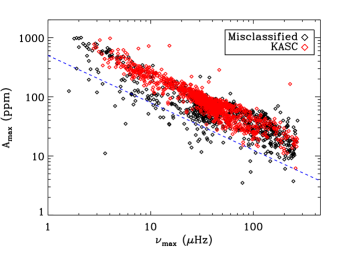
Figure 1.— Maximum amplitude per radial mode as a function of $\nu_{\rm max}$for the confirmed detections in our sample ( black symbols) and for $\sim$1200 known red giants ( red symbols). The blue dashed line represents the $5.10^{2}\times\mbox{$\nu_{\rm max}$}^{-0.8}$ below which we considered the stars with low $A_{\rm max}$.

Some of the oscillations detected could be due to a known red giant leaking onto the pixels of the dwarf. We searched for known red giants (either with detected oscillations or classified as red giants in the H14 catalog) that were within a radius of 1 arcmin (15 pixels) from the misclassified stars. The comparison of the power spectra of nearby known red giants with the misclassified stars showed that 52 stars out of the 875 stars with modes below Nyquist have the same power spectra and thus the mode detection results from pollution. We discarded these 52 stars from our sample. There are three additional stars (KIC 4907817, 8246648, and 9788579) where the power spectra look similar but the length of data available is different for the two samples of stars without any overlapping quarters making it more difficult to compare them. This leads to a final sample of confirmed misclassified stars of 854 stars: 820 stars with $\nu_{\rm max}$well below Nyquist, 31 near/superNyquist stars, and three stars that could result from pollution and that have the comment ’PP’ (for Possible Pollution).

In addition to the visual check of the J-band images for this subsample of stars, we also looked at the crowding of the whole sample of stars. The crowding is provided on the MAST and it is defined as the ratio of the target flux to the total flux in the optimal aperture. The optimal aperture is computed by the NASA Pre-search Data Conditioning (for more details see Jenkins et al., 2010). In this paper we define a crowding value of 1 when all the flux belongs to the main target. Since the satellite rolls every three months to keep its solar panels towards the Sun, the aperture and thus the crowding changes every quarter (as described in the NASA Kepler release notes). We computed the crowding as the median value of all the quarters. The values of crowding for each target are listed in Tables 1 and 3. Figure 2 shows the distribution of the crowding for the 854 stars. Most of the stars have a crowding larger than 75%, meaning that most of the flux is coming from the main target and the probability that there is a nearby star polluting the light curve is low. Stars with a crowding value below 75% should be considered very cautiously. They have the comment ’CR’ (for Crowding’) in the last column of Table 1.

Figure 2.— Histogram of the crowding as described in Section 3.2 for the 854 misclassified red giants.

Tables 1 and 2 list the seismic parameters obtained by the A2Z+ and SYD pipelines respectively. Table 3 gives the seismic parameters from A2Z+ for the near and super-Nyquist stars.

One of these stars, KIC 7292836, could be a seismic binary where we see two regions with modes. After changing the aperture for this star, by using a smaller number of pixels to produce the light curves, and inspecting the J-band image, we could not see a nearby star. We provide the seismic parameters of the two power excesses.

Table 1Seismic and fundamental parameters of the misclassified red giants obtained for the A2Z+ pipeline

KIC	$K_{p}$	$T_{\rm eff}$ (K)	$T^{*}_{\rm eff}$ (K)	$\Delta\nu$ ($\mu$Hz)	$\nu_{\rm max}$ ($\mu$Hz)	$\log g$	M∗ ($M_{\odot}$)	R∗ ($R_{\odot}$)	d (kpc)	Crowding	Flag
893233	11.4	4204${}^{+154}_{-156}$	4285${}^{+96}_{-96}$	1.03 $\pm$  0.18	6.1 $\pm$  0.4	1.67 $\pm$ 0.03	1.51 $\pm$  0.56	29.59 $\pm$  7.58	1.66${}^{+0.92}_{-0.31}$	0.98
1027110	12.1	4415${}^{+161}_{-149}$	4272${}^{+85}_{-85}$	1.13 $\pm$  0.11	6.6 $\pm$  0.4	1.71 $\pm$ 0.03	1.31 $\pm$  0.29	26.56 $\pm$  4.01	2.06${}^{+0.67}_{-0.13}$	0.98
1160684	14.9	4137${}^{+121}_{-144}$	4571${}^{+91}_{-91}$	3.59 $\pm$  0.10	27.5 $\pm$  1.4	2.34 $\pm$ 0.02	1.03 $\pm$  0.11	11.34 $\pm$  0.75	3.76${}^{+0.09}_{-0.08}$	0.91
1162220	11.2	4284${}^{+129}_{-134}$	4303${}^{+87}_{-86}$	1.68 $\pm$  0.05	11.1 $\pm$  0.7	1.94 $\pm$ 0.03	1.29 $\pm$  0.16	20.28 $\pm$  1.56	1.21${}^{+0.18}_{-0.07}$	0.99
1163114	12.7	4211${}^{+123}_{-138}$	4440${}^{+88}_{-88}$	1.91 $\pm$  0.20	14.2 $\pm$  0.7	2.05 $\pm$ 0.02	1.70 $\pm$  0.39	20.39 $\pm$  3.20	2.63${}^{+0.34}_{-0.26}$	0.97
1164356	14.1	5225${}^{+169}_{-135}$	5360${}^{+178}_{-125}$	3.33 $\pm$  0.09	27.8 $\pm$  1.8	2.38 $\pm$ 0.03	1.83 $\pm$  0.24	14.43 $\pm$  1.14	6.91${}^{+0.21}_{-0.25}$	0.74
1164584	14.3	4333${}^{+128}_{-133}$	4546${}^{+90}_{-90}$	3.35 $\pm$  0.12	28.8 $\pm$  1.4	2.36 $\pm$ 0.02	1.55 $\pm$  0.18	13.60 $\pm$  0.97	3.77${}^{+0.29}_{-0.54}$	0.95
1292147	15.2	4219${}^{+121}_{-145}$	4764${}^{+130}_{-106}$	8.12 $\pm$  0.28	87.2 $\pm$  4.2	2.85 $\pm$ 0.02	1.34 $\pm$  0.15	7.18 $\pm$  0.51	3.20${}^{+0.71}_{-0.30}$	0.91
1293587	14.9	4914${}^{+152}_{-126}$	4921${}^{+149}_{-98}$	16.67 $\pm$  0.17	253.8 $\pm$  23.8	3.32 $\pm$ 0.04	1.95 $\pm$  0.33	5.04 $\pm$  0.49	2.17${}^{+0.18}_{-0.12}$	0.86
1429629	15.2	4260${}^{+129}_{-146}$	4697${}^{+152}_{-93}$	6.28 $\pm$  0.19	63.0 $\pm$  3.1	2.71 $\pm$ 0.02	1.38 $\pm$  0.15	8.61 $\pm$  0.59	3.94${}^{+0.69}_{-0.32}$	0.94
1431059	13.1	4660${}^{+140}_{-122}$	4938${}^{+101}_{-98}$	13.62 $\pm$  0.47	171.3 $\pm$  7.6	3.15 $\pm$ 0.02	1.35 $\pm$  0.14	5.10 $\pm$  0.34	1.06${}^{+0.07}_{-0.07}$	0.98
1431599	12.3	4056${}^{+100}_{-115}$	4007${}^{+80}_{-80}$	0.53 $\pm$  0.28	2.3 $\pm$  0.2	1.24 $\pm$ 0.04	1.04 $\pm$  1.11	40.75 $\pm$  30.66	3.24${}^{+0.56}_{-0.21}$	0.98
1432022	14.8	5706${}^{+162}_{-184}$	4726${}^{+94}_{-94}$	0.92 $\pm$  0.01	4.5 $\pm$  0.3	1.56 $\pm$ 0.03	1.10 $\pm$  0.13	28.73 $\pm$  2.01	13.65${}^{+2.83}_{-0.77}$	0.93	PB
1576043	12.5	4012${}^{+120}_{-149}$	4176${}^{+83}_{-83}$	0.91 $\pm$  0.03	5.4 $\pm$  0.4	1.62 $\pm$ 0.03	1.65 $\pm$  0.24	33.13 $\pm$  2.94	2.76${}^{+0.46}_{-0.27}$	0.98
2010137	12.3	4019${}^{+123}_{-158}$	4253${}^{+85}_{-85}$	1.08 $\pm$  0.15	6.1 $\pm$  0.5	1.67 $\pm$ 0.04	1.23 $\pm$  0.39	26.81 $\pm$  5.72	2.18${}^{+1.19}_{-0.22}$	0.98
2010577	15.6	4703${}^{+181}_{-159}$	4773${}^{+116}_{-116}$	3.90 $\pm$  0.67	30.0 $\pm$  1.5	2.39 $\pm$ 0.02	1.03 $\pm$  0.36	10.71 $\pm$  2.66	6.78${}^{+4.03}_{-0.58}$	0.34	CR
2011870	13.2	3962${}^{+116}_{-161}$	4118${}^{+83}_{-83}$	0.76 $\pm$  0.01	4.7 $\pm$  0.2	1.55 $\pm$ 0.02	2.19 $\pm$  0.18	41.05 $\pm$  2.00	4.77${}^{+0.42}_{-0.25}$	0.97
2014684	11.8	4200${}^{+124}_{-138}$	4293${}^{+85}_{-85}$	1.05 $\pm$  0.11	5.8 $\pm$  0.4	1.65 $\pm$ 0.03	1.20 $\pm$  0.29	27.10 $\pm$  4.45	1.90${}^{+0.81}_{-0.19}$	0.99
2014737	15.6	5177${}^{+214}_{-160}$	5441${}^{+110}_{-110}$	3.93 $\pm$  0.67	27.4 $\pm$  1.7	2.38 $\pm$ 0.03	0.92 $\pm$  0.33	10.29 $\pm$  2.57	22.54${}^{+1.69}_{-2.06}$	0.35	CR
2159728	15.2	4787${}^{+189}_{-157}$	4936${}^{+196}_{-196}$	7.33 $\pm$  0.27	78.0 $\pm$  3.7	2.81 $\pm$ 0.02	1.52 $\pm$  0.18	8.02 $\pm$  0.61	4.71${}^{+0.26}_{-0.77}$	0.92
2167183	13.7	3987${}^{+126}_{-156}$	3975${}^{+79}_{-79}$	0.55 $\pm$  0.01	2.5 $\pm$  0.2	1.27 $\pm$ 0.04	1.14 $\pm$  0.17	40.97 $\pm$  3.49	5.40${}^{+0.32}_{-0.19}$	0.92
2284679	11.4	4895${}^{+149}_{-149}$	5004${}^{+126}_{-113}$	16.15 $\pm$  0.55	199.8 $\pm$  11.5	3.22 $\pm$ 0.03	1.11 $\pm$  0.14	4.26 $\pm$  0.33	0.56${}^{+0.04}_{-0.04}$	0.99
2297384	14.3	4350${}^{+125}_{-137}$	4625${}^{+92}_{-92}$	3.78 $\pm$  0.12	32.0 $\pm$  2.0	2.41 $\pm$ 0.03	1.35 $\pm$  0.17	11.98 $\pm$  0.94	3.42${}^{+0.34}_{-0.14}$	0.94
2297825	14.3	4240${}^{+123}_{-140}$	4668${}^{+93}_{-93}$	3.78 $\pm$  0.13	31.0 $\pm$  1.7	2.40 $\pm$ 0.03	1.24 $\pm$  0.15	11.65 $\pm$  0.87	3.37${}^{+0.19}_{-0.16}$	0.94
2308968	15.2	4988${}^{+156}_{-162}$	5097${}^{+152}_{-114}$	5.02 $\pm$  0.95	33.5 $\pm$  2.4	2.45 $\pm$ 0.03	0.57 $\pm$  0.23	7.46 $\pm$  2.07	9.23${}^{+0.50}_{-3.03}$	0.91
2309524	12.1	3839${}^{+121}_{-141}$	4060${}^{+102}_{-92}$	0.71 $\pm$  0.15	3.7 $\pm$  0.2	1.45 $\pm$ 0.03	1.38 $\pm$  0.60	36.77 $\pm$  11.18	2.09${}^{+0.56}_{-0.12}$	0.97
2422890	13.0	3898${}^{+125}_{-152}$	3899${}^{+88}_{-88}$	0.44 $\pm$  0.00	1.8 $\pm$  0.1	1.12 $\pm$ 0.03	1.01 $\pm$  0.10	45.65 $\pm$  2.72	4.93${}^{+0.20}_{-0.25}$	0.97
2436209	14.9	4248${}^{+128}_{-139}$	4716${}^{+102}_{-94}$	5.74 $\pm$  0.82	57.2 $\pm$  2.7	2.67 $\pm$ 0.02	1.49 $\pm$  0.44	9.37 $\pm$  1.95	4.31${}^{+0.34}_{-0.68}$	0.89
2436332	14.3	4187${}^{+126}_{-134}$	4498${}^{+90}_{-90}$	3.39 $\pm$  0.10	28.7 $\pm$  1.6	2.36 $\pm$ 0.03	1.44 $\pm$  0.17	13.17 $\pm$  0.94	3.71${}^{+0.30}_{-0.48}$	0.92
2436540	14.9	4386${}^{+123}_{-136}$	4652${}^{+116}_{-93}$	5.80 $\pm$  0.15	59.2 $\pm$  2.8	2.68 $\pm$ 0.02	1.55 $\pm$  0.16	9.44 $\pm$  0.59	3.74${}^{+0.45}_{-0.26}$	0.90
2436814	14.2	4219${}^{+126}_{-136}$	4488${}^{+93}_{-89}$	3.10 $\pm$  0.11	24.1 $\pm$  1.3	2.28 $\pm$ 0.02	1.22 $\pm$  0.15	13.21 $\pm$  0.99	3.62${}^{+0.47}_{-0.35}$	0.80
2436824	14.5	4214${}^{+126}_{-139}$	4429${}^{+88}_{-88}$	3.85 $\pm$  0.12	34.0 $\pm$  1.6	2.43 $\pm$ 0.02	1.41 $\pm$  0.15	12.00 $\pm$  0.79	5.90${}^{+0.33}_{-0.56}$	0.87
2437040	14.2	4209${}^{+118}_{-144}$	4490${}^{+89}_{-89}$	3.07 $\pm$  0.08	25.5 $\pm$  1.2	2.31 $\pm$ 0.02	1.50 $\pm$  0.15	14.25 $\pm$  0.88	3.82${}^{+0.22}_{-0.34}$	0.72
2437402	14.7	4315${}^{+124}_{-139}$	4712${}^{+104}_{-94}$	4.81 $\pm$  0.16	46.1 $\pm$  2.3	2.57 $\pm$ 0.02	1.58 $\pm$  0.18	10.75 $\pm$  0.76	4.11${}^{+0.14}_{-0.17}$	0.69
2437507	14.1	4156${}^{+122}_{-132}$	4493${}^{+95}_{-95}$	2.62 $\pm$  0.01	20.6 $\pm$  1.1	2.21 $\pm$ 0.02	1.49 $\pm$  0.14	15.81 $\pm$  0.88	4.00${}^{+0.09}_{-0.34}$	0.94
2437539	14.6	4178${}^{+119}_{-137}$	4683${}^{+104}_{-93}$	4.88 $\pm$  0.17	46.8 $\pm$  2.3	2.58 $\pm$ 0.02	1.54 $\pm$  0.18	10.57 $\pm$  0.75	3.87${}^{+0.18}_{-0.47}$	0.94
2437589	14.3	4197${}^{+119}_{-138}$	4729${}^{+94}_{-94}$	4.63 $\pm$  0.16	46.9 $\pm$  2.4	2.58 $\pm$ 0.02	1.95 $\pm$  0.22	11.83 $\pm$  0.85	3.52${}^{+0.21}_{-0.13}$	0.95
2437653	15.2	4386${}^{+130}_{-129}$	4818${}^{+155}_{-155}$	7.03 $\pm$  0.21	74.1 $\pm$  3.4	2.78 $\pm$ 0.02	1.49 $\pm$  0.16	8.18 $\pm$  0.54	4.25${}^{+0.33}_{-0.71}$	0.86
2437698	14.2	4269${}^{+123}_{-145}$	4660${}^{+95}_{-95}$	3.74 $\pm$  0.12	31.8 $\pm$  2.1	2.41 $\pm$ 0.03	1.39 $\pm$  0.19	12.20 $\pm$  0.99	3.37${}^{+0.41}_{-0.15}$	0.94
2437805	14.2	4178${}^{+117}_{-139}$	4673${}^{+95}_{-95}$	3.85 $\pm$  0.50	31.8 $\pm$  1.8	2.41 $\pm$ 0.03	1.25 $\pm$  0.35	11.53 $\pm$  2.22	3.32${}^{+0.66}_{-0.22}$	0.93
2437816	14.0	4146${}^{+125}_{-131}$	4419${}^{+88}_{-88}$	2.38 $\pm$  0.07	17.9 $\pm$  0.9	2.15 $\pm$ 0.02	1.40 $\pm$  0.15	16.52 $\pm$  1.10	3.79${}^{+0.41}_{-0.50}$	0.91
2438038	15.0	4315${}^{+123}_{-142}$	4663${}^{+103}_{-93}$	6.15 $\pm$  0.19	62.9 $\pm$  3.0	2.71 $\pm$ 0.02	1.48 $\pm$  0.16	8.93 $\pm$  0.59	3.70${}^{+0.34}_{-0.27}$	0.91
2438094	15.3	4356${}^{+124}_{-138}$	4369${}^{+87}_{-87}$	1.58 $\pm$  0.04	9.9 $\pm$  0.7	1.89 $\pm$ 0.03	1.20 $\pm$  0.16	20.61 $\pm$  1.66	9.02${}^{+0.82}_{-0.65}$	0.82
2441711	14.8	4777${}^{+187}_{-163}$	4696${}^{+93}_{-93}$	4.00 $\pm$  0.11	33.3 $\pm$  3.6	2.43 $\pm$ 0.05	1.24 $\pm$  0.24	11.21 $\pm$  1.30	4.91${}^{+0.24}_{-0.19}$	0.94
2448727	15.3	4497${}^{+168}_{-156}$	4645${}^{+92}_{-92}$	4.38 $\pm$  0.13	38.2 $\pm$  2.3	2.49 $\pm$ 0.03	1.28 $\pm$  0.16	10.67 $\pm$  0.80	5.53${}^{+0.20}_{-0.59}$	0.92
2556387	11.1	3445${}^{+117}_{-113}$	4464${}^{+89}_{-89}$	2.21 $\pm$  0.06	19.5 $\pm$  1.0	2.19 $\pm$ 0.02	2.47 $\pm$  0.26	20.97 $\pm$  1.38	1.44${}^{+0.10}_{-0.08}$	0.99
2569360	14.2	4187${}^{+122}_{-138}$	4424${}^{+90}_{-88}$	2.75 $\pm$  0.10	21.3 $\pm$  1.1	2.22 $\pm$ 0.02	1.33 $\pm$  0.16	14.73 $\pm$  1.09	3.71${}^{+0.45}_{-0.45}$	0.94
2570094	15.0	4386${}^{+126}_{-135}$	4799${}^{+147}_{-132}$	6.49 $\pm$  0.22	68.4 $\pm$  3.2	2.75 $\pm$ 0.02	1.60 $\pm$  0.18	8.84 $\pm$  0.62	4.19${}^{+0.40}_{-0.65}$	0.83
2570518	14.7	4399${}^{+130}_{-127}$	4566${}^{+91}_{-91}$	4.94 $\pm$  0.15	46.1 $\pm$  2.7	2.57 $\pm$ 0.03	1.35 $\pm$  0.16	10.04 $\pm$  0.74	3.57${}^{+0.31}_{-0.21}$	0.83
2571093	12.7	3815${}^{+114}_{-139}$	3900${}^{+78}_{-78}$	0.48 $\pm$  0.48	2.1 $\pm$  0.1	1.19 $\pm$ 0.02	1.13 $\pm$  2.27	44.75 $\pm$  63.33	3.21${}^{+0.39}_{-0.19}$	0.97
2578811	12.0	3685${}^{+110}_{-139}$	3912${}^{+80}_{-78}$	0.35 $\pm$  0.04	1.6 $\pm$  0.1	1.07 $\pm$ 0.03	1.78 $\pm$  0.45	64.22 $\pm$  11.17	2.89${}^{+1.04}_{-0.30}$	0.98
2585447	14.8	5403${}^{+168}_{-137}$	5305${}^{+388}_{-388}$	1.42 $\pm$  0.05	8.3 $\pm$  0.5	1.85 $\pm$ 0.04	1.45 $\pm$  0.22	23.57 $\pm$  2.21	19.55${}^{+0.80}_{-8.41}$	0.56	CR
2708445	15.0	4182${}^{+120}_{-135}$	4584${}^{+91}_{-91}$	6.11 $\pm$  0.18	60.5 $\pm$  3.0	2.69 $\pm$ 0.02	1.32 $\pm$  0.14	8.63 $\pm$  0.57	3.57${}^{+0.22}_{-0.25}$	0.90
2713304	15.9	3989${}^{+50}_{-50}$	4381${}^{+108}_{-97}$	1.23 $\pm$  0.20	6.9 $\pm$  0.6	1.73 $\pm$ 0.04	1.11 $\pm$  0.40	23.73 $\pm$  5.85	12.21${}^{+7.20}_{-1.35}$	0.37	CR
2715419	15.1	5151${}^{+193}_{-155}$	5026${}^{+100}_{-100}$	1.88 $\pm$  0.01	9.5 $\pm$  0.7	1.90 $\pm$ 0.03	0.65 $\pm$  0.09	14.98 $\pm$  1.13	8.76${}^{+0.39}_{-0.18}$	0.88
2721453	15.1	4819${}^{+154}_{-134}$	4882${}^{+97}_{-97}$	15.44 $\pm$  0.05	214.1 $\pm$  35.3	3.25 $\pm$ 0.08	1.57 $\pm$  0.45	4.93 $\pm$  0.82	2.25${}^{+0.15}_{-0.13}$	0.92
2845610	9.3	5095${}^{+151}_{-129}$	5051${}^{+101}_{-101}$	6.97 $\pm$  0.14	90.1 $\pm$  5.2	2.88 $\pm$ 0.03	2.97 $\pm$  0.33	10.36 $\pm$  0.68	0.46${}^{+0.01}_{-0.02}$	1.00
2846051	10.2	4203${}^{+100}_{-121}$	4297${}^{+88}_{-88}$	1.15 $\pm$  0.04	6.8 $\pm$  0.4	1.72 $\pm$ 0.03	1.35 $\pm$  0.17	26.50 $\pm$  2.07	0.96${}^{+0.19}_{-0.07}$	1.00
…

Table 2Seismic and fundamental parameters of the misclassified red giants obtained for the SYD pipeline

KIC	$T^{*}_{\rm eff}$ (K)	$\Delta\nu$ ($\mu$Hz)	$\nu_{\rm max}$ ($\mu$Hz)	$\log g$	M∗ ($M_{\odot}$)	R∗ ($R_{\odot}$)	d (kpc)
893233	4276${}^{+89}_{-156}$	1.17 $\pm$  0.02	6.1 $\pm$  0.1	1.67 $\pm$ 0.01	0.90 $\pm$  0.04	22.87 $\pm$  0.71	1.44${}^{+0.06}_{-0.03}$
1027110	4241${}^{+87}_{-149}$	1.15 $\pm$  0.01	6.7 $\pm$  0.2	1.71 $\pm$ 0.02	1.24 $\pm$  0.09	25.79 $\pm$  1.12	2.13${}^{+0.14}_{-0.12}$
1160684	4555${}^{+91}_{-144}$	3.56 $\pm$  0.05	27.3 $\pm$  0.6	2.34 $\pm$ 0.01	1.04 $\pm$  0.06	11.43 $\pm$  0.39	3.77${}^{+0.09}_{-0.08}$
1162220	4278${}^{+106}_{-134}$	1.67 $\pm$  0.01	11.0 $\pm$  0.4	1.93 $\pm$ 0.02	1.28 $\pm$  0.09	20.30 $\pm$  0.80	1.22${}^{+0.10}_{-0.05}$
1163114	4419${}^{+90}_{-138}$	1.89 $\pm$  0.01	14.3 $\pm$  0.5	2.05 $\pm$ 0.02	1.80 $\pm$  0.12	20.96 $\pm$  0.81	2.61${}^{+0.14}_{-0.10}$
1164356	5471${}^{+269}_{-135}$	3.33 $\pm$  0.01	27.7 $\pm$  0.6	2.38 $\pm$ 0.02	1.85 $\pm$  0.13	14.47 $\pm$  0.60	6.15${}^{+0.81}_{-0.68}$
1164584	4554${}^{+95}_{-133}$	3.36 $\pm$  0.01	28.4 $\pm$  0.5	2.36 $\pm$ 0.01	1.49 $\pm$  0.06	13.40 $\pm$  0.30	3.76${}^{+0.08}_{-0.21}$
1292147	4701${}^{+94}_{-145}$	8.12 $\pm$  0.02	88.0 $\pm$  0.9	2.85 $\pm$ 0.01	1.35 $\pm$  0.04	7.20 $\pm$  0.13	3.12${}^{+0.13}_{-0.11}$
1429629	4664${}^{+93}_{-146}$	6.27 $\pm$  0.01	62.7 $\pm$  0.7	2.71 $\pm$ 0.01	1.36 $\pm$  0.04	8.57 $\pm$  0.16	2.12${}^{+0.12}_{-0.14}$
1431059	4912${}^{+98}_{-122}$	13.64 $\pm$  0.02	169.5 $\pm$  0.9	3.15 $\pm$ 0.01	1.29 $\pm$  0.03	5.02 $\pm$  0.08	3.84${}^{+0.18}_{-0.10}$
1431599	3989${}^{+79}_{-115}$	0.53 $\pm$  0.01	2.3 $\pm$  0.1	1.24 $\pm$ 0.01	1.01 $\pm$  0.07	40.17 $\pm$  1.63	1.05${}^{+0.03}_{-0.03}$
1432022	4723${}^{+94}_{-184}$	0.90 $\pm$  0.01	4.4 $\pm$  0.2	1.55 $\pm$ 0.02	1.08 $\pm$  0.11	28.98 $\pm$  1.71	3.24${}^{+0.15}_{-0.15}$
1576043	4168${}^{+83}_{-149}$	0.93 $\pm$  0.01	5.3 $\pm$  0.3	1.61 $\pm$ 0.03	1.44 $\pm$  0.17	31.31 $\pm$  2.11	13.71${}^{+1.43}_{-0.71}$
2010137	4203${}^{+95}_{-158}$	1.08 $\pm$  0.01	6.0 $\pm$  0.1	1.66 $\pm$ 0.01	1.12 $\pm$  0.05	25.96 $\pm$  0.71	2.65${}^{+0.42}_{-0.17}$
2010577	4749${}^{+95}_{-159}$	3.89 $\pm$  0.05	29.9 $\pm$  0.6	2.39 $\pm$ 0.01	1.02 $\pm$  0.05	10.71 $\pm$  0.33	2.18${}^{+0.15}_{-0.08}$
2011870	4102${}^{+84}_{-161}$	0.77 $\pm$  0.01	4.6 $\pm$  0.1	1.54 $\pm$ 0.01	1.89 $\pm$  0.08	38.54 $\pm$  0.99	6.68${}^{+0.30}_{-0.30}$
2014684	4282${}^{+85}_{-138}$	1.09 $\pm$  0.02	5.8 $\pm$  0.1	1.65 $\pm$ 0.01	1.03 $\pm$  0.06	25.02 $\pm$  0.91	4.64${}^{+0.14}_{-0.19}$
2014737	5306${}^{+106}_{-160}$	3.79 $\pm$  0.10	27.9 $\pm$  0.8	2.38 $\pm$ 0.01	1.10 $\pm$  0.09	11.17 $\pm$  0.56	1.84${}^{+0.08}_{-0.08}$
2159728	4735${}^{+94}_{-157}$	7.32 $\pm$  0.02	78.0 $\pm$  0.7	2.80 $\pm$ 0.01	1.43 $\pm$  0.04	7.87 $\pm$  0.14	13.11${}^{+1.40}_{-0.93}$
2167183	3993${}^{+79}_{-156}$	0.57 $\pm$  0.02	2.5 $\pm$  0.0	1.27 $\pm$ 0.01	1.03 $\pm$  0.08	38.87 $\pm$  2.00	3.91${}^{+0.17}_{-0.17}$
2284679	4946${}^{+143}_{-149}$	16.15 $\pm$  0.02	197.8 $\pm$  1.0	3.22 $\pm$ 0.01	1.06 $\pm$  0.04	4.20 $\pm$  0.09	5.23${}^{+0.29}_{-0.20}$
2297384	4597${}^{+92}_{-137}$	3.79 $\pm$  0.03	31.2 $\pm$  1.1	2.40 $\pm$ 0.02	1.22 $\pm$  0.08	11.57 $\pm$  0.46	0.52${}^{+0.03}_{-0.02}$
2297825	4654${}^{+93}_{-140}$	3.82 $\pm$  0.03	30.5 $\pm$  0.8	2.39 $\pm$ 0.01	1.13 $\pm$  0.06	11.20 $\pm$  0.36	3.42${}^{+0.12}_{-0.10}$
2308968	5443${}^{+108}_{-162}$	5.03 $\pm$  0.11	34.1 $\pm$  0.6	2.47 $\pm$ 0.01	0.66 $\pm$  0.04	7.80 $\pm$  0.29	3.40${}^{+0.08}_{-0.12}$
2309524	4021${}^{+100}_{-141}$	0.71 $\pm$  0.01	3.8 $\pm$  0.1	1.45 $\pm$ 0.01	1.43 $\pm$  0.09	37.10 $\pm$  1.44	5.19${}^{+0.10}_{-0.10}$
2422890	3874${}^{+77}_{-152}$	0.42 $\pm$  0.04	1.7 $\pm$  0.0	1.09 $\pm$ 0.01	0.97 $\pm$  0.18	46.27 $\pm$  6.04	2.29${}^{+0.27}_{-0.15}$
2436209	4668${}^{+93}_{-139}$	5.74 $\pm$  0.01	57.2 $\pm$  0.6	2.66 $\pm$ 0.01	1.46 $\pm$  0.04	9.31 $\pm$  0.16	4.96${}^{+0.41}_{-0.20}$
2436332	4498${}^{+90}_{-134}$	3.40 $\pm$  0.01	28.5 $\pm$  0.8	2.35 $\pm$ 0.01	1.40 $\pm$  0.07	13.02 $\pm$  0.40	3.76${}^{+0.13}_{-0.17}$
2436540	4652${}^{+93}_{-136}$	5.80 $\pm$  0.01	58.3 $\pm$  0.8	2.67 $\pm$ 0.01	1.49 $\pm$  0.05	9.31 $\pm$  0.19	3.67${}^{+0.27}_{-0.13}$
2436814	4514${}^{+90}_{-136}$	3.13 $\pm$  0.01	24.4 $\pm$  0.4	2.29 $\pm$ 0.01	1.23 $\pm$  0.05	13.17 $\pm$  0.30	3.74${}^{+0.18}_{-0.16}$
2436824	4417${}^{+88}_{-139}$	3.85 $\pm$  0.01	34.0 $\pm$  0.3	2.43 $\pm$ 0.01	1.40 $\pm$  0.04	11.99 $\pm$  0.21	3.61${}^{+0.13}_{-0.18}$
2437040	4491${}^{+89}_{-144}$	3.08 $\pm$  0.01	25.5 $\pm$  0.5	2.31 $\pm$ 0.01	1.48 $\pm$  0.06	14.18 $\pm$  0.34	5.77${}^{+0.32}_{-0.29}$
2437402	4688${}^{+221}_{-139}$	4.81 $\pm$  0.01	45.7 $\pm$  0.9	2.57 $\pm$ 0.02	1.53 $\pm$  0.10	10.65 $\pm$  0.42	3.78${}^{+0.09}_{-0.23}$
2437507	4486${}^{+89}_{-132}$	2.60 $\pm$  0.01	20.5 $\pm$  0.4	2.21 $\pm$ 0.01	1.50 $\pm$  0.06	15.91 $\pm$  0.39	4.06${}^{+0.21}_{-0.27}$
2437539	4715${}^{+194}_{-137}$	4.90 $\pm$  0.01	46.8 $\pm$  0.6	2.58 $\pm$ 0.01	1.53 $\pm$  0.08	10.52 $\pm$  0.34	3.95${}^{+0.13}_{-0.26}$
2437589	4720${}^{+94}_{-138}$	4.61 $\pm$  0.01	46.6 $\pm$  1.0	2.58 $\pm$ 0.01	1.94 $\pm$  0.09	11.86 $\pm$  0.30	3.73${}^{+0.30}_{-0.18}$
2437653	4688${}^{+115}_{-129}$	7.01 $\pm$  0.01	73.8 $\pm$  0.7	2.78 $\pm$ 0.01	1.43 $\pm$  0.05	8.09 $\pm$  0.16	3.66${}^{+0.11}_{-0.18}$
2437698	4643${}^{+93}_{-145}$	3.76 $\pm$  0.02	30.8 $\pm$  1.6	2.40 $\pm$ 0.02	1.24 $\pm$  0.11	11.70 $\pm$  0.62	3.68${}^{+0.22}_{-0.15}$
2437805	4601${}^{+94}_{-139}$	3.79 $\pm$  0.04	31.7 $\pm$  0.9	2.41 $\pm$ 0.01	1.29 $\pm$  0.08	11.79 $\pm$  0.43	3.35${}^{+0.19}_{-0.13}$
2437816	4421${}^{+106}_{-131}$	2.35 $\pm$  0.01	17.7 $\pm$  0.3	2.14 $\pm$ 0.01	1.44 $\pm$  0.06	16.83 $\pm$  0.41	3.33${}^{+0.17}_{-0.08}$
2438038	4647${}^{+92}_{-142}$	6.14 $\pm$  0.01	62.6 $\pm$  0.7	2.70 $\pm$ 0.01	1.46 $\pm$  0.05	8.89 $\pm$  0.16	3.76${}^{+0.15}_{-0.17}$
2438094	4373${}^{+88}_{-138}$	1.58 $\pm$  0.01	10.0 $\pm$  0.5	1.89 $\pm$ 0.02	1.23 $\pm$  0.11	20.76 $\pm$  1.10	3.73${}^{+0.10}_{-0.15}$
2441711	4678${}^{+93}_{-163}$	4.00 $\pm$  0.04	35.4 $\pm$  1.2	2.46 $\pm$ 0.02	1.47 $\pm$  0.10	11.88 $\pm$  0.46	9.00${}^{+0.32}_{-0.64}$
2448727	4602${}^{+126}_{-156}$	4.38 $\pm$  0.01	38.5 $\pm$  0.8	2.49 $\pm$ 0.01	1.28 $\pm$  0.06	10.68 $\pm$  0.31	4.95${}^{+0.30}_{-0.15}$
2556387	4465${}^{+89}_{-113}$	2.23 $\pm$  0.02	19.4 $\pm$  0.9	2.19 $\pm$ 0.02	2.35 $\pm$  0.20	20.48 $\pm$  1.02	5.04${}^{+0.57}_{-0.16}$
2569360	4393${}^{+111}_{-138}$	2.75 $\pm$  0.01	21.5 $\pm$  0.4	2.23 $\pm$ 0.01	1.36 $\pm$  0.06	14.85 $\pm$  0.41	1.44${}^{+0.10}_{-0.05}$
2570094	4722${}^{+129}_{-135}$	6.50 $\pm$  0.02	67.8 $\pm$  0.8	2.74 $\pm$ 0.01	1.51 $\pm$  0.06	8.66 $\pm$  0.20	3.68${}^{+0.14}_{-0.16}$
2570518	4563${}^{+91}_{-127}$	4.93 $\pm$  0.01	45.9 $\pm$  0.6	2.56 $\pm$ 0.01	1.34 $\pm$  0.04	10.01 $\pm$  0.19	3.79${}^{+0.26}_{-0.21}$
2571093	3905${}^{+86}_{-139}$	0.45 $\pm$  0.05	2.1 $\pm$  0.0	1.19 $\pm$ 0.01	1.44 $\pm$  0.32	50.61 $\pm$  8.02	3.62${}^{+0.13}_{-0.09}$
2578811	3910${}^{+78}_{-139}$	0.36 $\pm$  0.02	1.6 $\pm$  0.2	1.08 $\pm$ 0.06	1.71 $\pm$  0.41	62.61 $\pm$  9.00	3.25${}^{+0.34}_{-0.19}$
2585447	4888${}^{+432}_{-137}$	1.43 $\pm$  0.02	8.2 $\pm$  0.6	1.83 $\pm$ 0.04	1.21 $\pm$  0.20	22.13 $\pm$  2.17	2.99${}^{+0.68}_{-0.25}$
2708445	4576${}^{+91}_{-135}$	6.09 $\pm$  0.01	60.2 $\pm$  0.6	2.68 $\pm$ 0.01	1.31 $\pm$  0.04	8.63 $\pm$  0.15	10.50${}^{+8.06}_{-1.42}$
2713304	4380${}^{+109}_{-50}$	1.14 $\pm$  0.02	6.6 $\pm$  1.1	1.72 $\pm$ 0.08	1.33 $\pm$  0.39	26.53 $\pm$  4.50	3.63${}^{+0.11}_{-0.13}$
2715419	4999${}^{+100}_{-155}$	1.84 $\pm$  0.03	9.5 $\pm$  0.3	1.90 $\pm$ 0.02	0.70 $\pm$  0.05	15.54 $\pm$  0.64	13.34${}^{+4.44}_{-1.48}$
2845610	5055${}^{+101}_{-129}$	7.13 $\pm$  0.03	93.6 $\pm$  6.9	2.90 $\pm$ 0.03	3.04 $\pm$  0.40	10.29 $\pm$  0.77	8.86${}^{+0.25}_{-0.18}$
2846051	4322${}^{+86}_{-121}$	1.10 $\pm$  0.01	6.8 $\pm$  0.2	1.73 $\pm$ 0.01	1.65 $\pm$  0.10	29.20 $\pm$  1.04	2.24${}^{+0.13}_{-0.13}$
2846944	4326${}^{+98}_{-145}$	1.42 $\pm$  0.01	7.9 $\pm$  0.3	1.79 $\pm$ 0.02	0.93 $\pm$  0.07	20.31 $\pm$  0.85	0.46${}^{+0.01}_{-0.01}$
2847114	4256${}^{+85}_{-120}$	1.33 $\pm$  0.02	7.6 $\pm$  0.3	1.77 $\pm$ 0.02	1.03 $\pm$  0.07	21.95 $\pm$  0.92	1.16${}^{+0.05}_{-0.05}$
2850913	4619${}^{+92}_{-135}$	5.23 $\pm$  0.01	49.3 $\pm$  0.7	2.60 $\pm$ 0.01	1.34 $\pm$  0.05	9.62 $\pm$  0.19	1.80${}^{+0.07}_{-0.04}$
2853089	4972${}^{+99}_{-171}$	10.78 $\pm$  0.04	122.1 $\pm$  1.4	3.01 $\pm$ 0.01	1.26 $\pm$  0.04	5.82 $\pm$  0.11	2.36${}^{+0.12}_{-0.10}$
2853469	3912${}^{+88}_{-152}$	0.44 $\pm$  0.01	1.9 $\pm$  0.0	1.15 $\pm$ 0.01	1.19 $\pm$  0.09	48.17 $\pm$  2.57	2.15${}^{+0.07}_{-0.07}$
2861062	4973${}^{+168}_{-145}$	1.86 $\pm$  0.01	12.9 $\pm$  0.6	2.03 $\pm$ 0.02	1.68 $\pm$  0.15	20.71 $\pm$  1.06	5.35${}^{+0.34}_{-0.34}$
2865296	4722${}^{+94}_{-122}$	3.78 $\pm$  0.14	27.7 $\pm$  0.6	2.35 $\pm$ 0.01	0.90 $\pm$  0.08	10.48 $\pm$  0.60	3.25${}^{+0.25}_{-0.19}$
2986860	4449${}^{+89}_{-170}$	1.49 $\pm$  0.02	9.8 $\pm$  0.7	1.89 $\pm$ 0.03	1.54 $\pm$  0.19	23.36 $\pm$  1.65	14.30${}^{+1.00}_{-0.70}$
…

Table 3Properties of the red giants with modes near or above the Nyquist frequency from the A2Z+ pipeline

KIC	$K_{p}$	$T_{\rm eff}$ (K)	$\Delta\nu$ ($\mu$Hz)	$\nu_{\rm max}$ ($\mu$Hz)	$\log g$	Crowding
1296817	12.2	4931 $\pm$  98	23.12 $\pm$  0.65	325.0 $\pm$ 22.5	3.43 $\pm$ 0.03	0.99
3215881	12.0	5045 $\pm$  100	20.98 $\pm$  0.71	285.0 $\pm$ 23.1	3.38 $\pm$ 0.03	1.00
3831261	14.2	4921 $\pm$  98	14.34 $\pm$  0.08	285.0 $\pm$ 20.3	3.37 $\pm$ 0.03	0.99
3947028	15.4	4750 $\pm$  95	18.88 $\pm$  0.20	285.0 $\pm$ 20.3	3.37 $\pm$ 0.03	0.99
4556618	14.1	4911 $\pm$  98	19.20 $\pm$  0.81	285.0 $\pm$ 20.3	3.37 $\pm$ 0.03	0.99
4920027	15.3	5180 $\pm$  103	17.16 $\pm$  0.98	285.0 $\pm$ 20.3	3.39 $\pm$ 0.03	0.94
5184359	14.1	5158 $\pm$  103	19.87 $\pm$  0.81	285.0 $\pm$ 20.3	3.38 $\pm$ 0.03	1.00
5620827	11.1	4998 $\pm$  99	19.53 $\pm$  2.22	285.0 $\pm$ 20.3	3.38 $\pm$ 0.03	1.00
5702338	14.6	5078 $\pm$  101	20.60 $\pm$  0.36	285.0 $\pm$ 20.3	3.38 $\pm$ 0.03	0.98
6263730	11.8	5151 $\pm$  103	20.23 $\pm$  0.75	285.0 $\pm$ 20.3	3.38 $\pm$ 0.03	1.00
6284113	11.5	4975 $\pm$  99	18.57 $\pm$  0.38	285.0 $\pm$ 20.3	3.38 $\pm$ 0.03	0.99
6591545	14.9	5132 $\pm$  102	18.57 $\pm$  0.28	285.0 $\pm$ 20.3	3.38 $\pm$ 0.03	1.00
7122721	13.4	5029 $\pm$  100	17.16 $\pm$  0.34	285.0 $\pm$ 20.3	3.38 $\pm$ 0.03	0.60
7550798	13.9	5075 $\pm$  101	26.34 $\pm$  0.93	370.0 $\pm$ 20.3	3.49 $\pm$ 0.03	0.99
7678714	13.6	5093 $\pm$  101	20.91 $\pm$  0.24	285.0 $\pm$ 20.3	3.38 $\pm$ 0.03	0.98
7732398	13.9	5385 $\pm$  107	19.20 $\pm$  0.50	285.0 $\pm$ 20.3	3.39 $\pm$ 0.03	0.98
8037501	13.4	4840 $\pm$  96	17.70 $\pm$  0.52	285.0 $\pm$ 20.3	3.37 $\pm$ 0.03	0.97
8417876	14.3	5228 $\pm$  104	20.60 $\pm$  0.50	285.0 $\pm$ 20.3	3.39 $\pm$ 0.03	0.99
8553989	12.5	5132 $\pm$  102	24.10 $\pm$  0.55	285.0 $\pm$ 20.3	3.38 $\pm$ 0.03	0.99
9095475	14.7	5035 $\pm$  100	21.37 $\pm$  0.74	285.0 $\pm$ 20.3	3.38 $\pm$ 0.03	0.98
9221660	12.4	5160 $\pm$  103	19.87 $\pm$  0.49	285.0 $\pm$ 20.3	3.38 $\pm$ 0.03	1.00
9637300	13.6	5095 $\pm$  101	23.60 $\pm$  0.96	335.0 $\pm$ 20.3	3.45 $\pm$ 0.03	1.00
9639069	14.4	5193 $\pm$  103	19.53 $\pm$  0.30	285.0 $\pm$ 20.3	3.39 $\pm$ 0.03	1.00
9698043	13.9	5178 $\pm$  103	22.66 $\pm$  0.41	285.0 $\pm$ 20.3	3.39 $\pm$ 0.03	0.99
9706054	14.3	5205 $\pm$  104	21.78 $\pm$  0.53	285.0 $\pm$ 20.3	3.39 $\pm$ 0.03	0.97
10264711	14.3	5078 $\pm$  101	20.60 $\pm$  0.49	285.0 $\pm$ 20.3	3.38 $\pm$ 0.03	0.99
11138117	14.6	5159 $\pm$  103	22.21 $\pm$  0.34	285.0 $\pm$ 20.3	3.38 $\pm$ 0.03	1.00
11181529	13.3	5209 $\pm$  104	20.23 $\pm$  0.48	285.0 $\pm$ 20.3	3.39 $\pm$ 0.03	1.00
11250788	11.1	5375 $\pm$  107	19.87 $\pm$  0.64	285.0 $\pm$ 20.3	3.39 $\pm$ 0.03	1.00
11443679	13.7	5361 $\pm$  107	19.20 $\pm$  0.39	285.0 $\pm$ 20.3	3.39 $\pm$ 0.03	0.96
11666333	13.8	5254 $\pm$  105	19.20 $\pm$  0.46	285.0 $\pm$ 25.0	3.39 $\pm$ 0.03	0.96

3.3. Revised Effective Temperatures and Distances

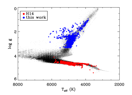
Figure 3.— HR diagram of the stars cataloged in H14 (black dots). Stars in our sample are overplotted with colored circles: the old stellar parameters are represented in red symbols and the parameters derived in this work (i.e. seismic $\log g$ and revised $T_{\rm eff}$) are represented with blue symbols.

Previous estimates of effective temperatures for this sample were mostly based on matching broadband photometry to models assuming a simple reddening law as part of the classifications for the KIC. If the stars are indeed giants instead of dwarfs, these temperatures will be underestimated since the stars are more distant and therefore more reddened than initially assumed.

To determine revised temperatures and distances for the sample we used broadband photometry, asteroseismic observables, and a grid of Parsec isochrones (Bressan et al., 2012). The grid ranges from 0.5–14 Gyr with a stepsize of 0.5 Gyr and $Z=0.0001-0.03$ with a stepsize of 0.0001 (corresponding to metallicities between $\mbox{$\rm{[Fe/H]}$}=-2.18$ and $\mbox{$\rm{[Fe/H]}$}=+0.42$), and was calculated with a Reimers mass loss parameters set to $\eta=0.2$.

Given a set of observables $x=\{J-K,H-K,g-r,r-i,\mbox{$\nu_{\rm max}$},\mbox{$\Delta\nu$}\}$ with Gaussian uncertainties $\sigma_{x}$ and a set of intrinsic parameters $y=\{\rm age,\ [Fe/H],\ mass\}$, we calculated the posterior probability of the observed star having intrinsic parameters $y$ as:

$$\begin{split}p(y|x)\propto p(y)p(x|y)\propto p(y)\prod_{i}\exp{\left(-\frac{(x_{i}-x_{i}(y))^{2}}{2\sigma_{x,i}^{2}}\right)}\>.\end{split}$$ (1)

For $p(y)$ we adopt a flat prior on age and mass, and a metallicity prior derived from the Geneva Copenhagen survey (Casagrande et al., 2011), which has been shown to agree well with the metallicity distribution of Kepler targets (Dong et al., 2014). We used 2MASS $J-H$ and $H-K$ colors if all three bands have the highest photometric quality flag (Qflg=’AAA’), and KIC $g-r,r-i$ colors otherwise. For the KIC photometry we interpolated uncertainties as a function of $Kp$ using typical values taken from Figure 3 in Brown et al. (2011). Nine stars did not have all the colors available or a not high-enough quality flag so they do not have results from this method. Model colors and distances are calculated from absolute magnitudes, which are reddened using the 3D extinction map by Amôres & Lépine (2005) for distances corresponding to the apparent magnitude (either $J$-band or $g$-band) and galactic coordinates of a given target. Values for $\nu_{\rm max}$ and $\Delta\nu$ values for each model were calculated using the scaling relations (Kjeldsen & Bedding, 1995), assuming solar reference values of $\mbox{$\nu_{\rm max}$}=3090\mbox{$\mu$Hz}$ and $\mbox{$\Delta\nu$}=135.1\mbox{$\mu$Hz}$ (Huber et al., 2011). Temperatures and distances were then derived from the median and $1\sigma$ confidence interval of the probability distribution function obtained by integrating $p(y|x)$ along the isochrone grid, weighted by local grid spacing in mass, age and metallicity (Serenelli et al., 2013). We note that we assumed that the targets were single stars when deriving the distances but that effect should be small.

For the stars with $\nu_{\rm max}$ below the Nyquist frequency, we computed the mass, radius, and $\log g$ using the scaling relations along with the updated effective temperature. The stellar parameters are all listed in Tables 1 and 2 , respectively for the A2Z+ and the SYD pipelines. For the stars with modes near or above the Nyquist frequency, we only computed the $\log g$ as we only have a very rough estimate of $\nu_{\rm max}$. The seismic parameters for this subsample of stars are given in Table 3. Figure 3 shows a $\log g$ versus $T_{\rm eff}$ diagram comparing the positions of the sample before and after the re-derivation of $\log g$ and $T_{\rm eff}$. Note that $\log g$ values for the sample were calculated using the $\nu_{\rm max}$ scaling relations with the revised $T_{\rm eff}$. As expected, most stars shift to hotter temperatures since the de-reddened colors assuming larger distances are bluer than de-reddened colors assuming that the stars are dwarfs.

3.4. Mixed modes and evolutionary stage

As stars evolve to become red giants the acoustic modes in the stellar envelope start to couple with the gravity modes in the core, which leads to the so-called mixed modes (Dupret et al., 2009). Mixed modes have been observed in several thousands of giants in the Kepler field (e.g. Beck et al., 2011; Bedding et al., 2011; Mosser et al., 2012; Stello et al., 2013). Because of their partly gravity-mode nature, they are sensitive to the stellar core properties, and in particular whether a star is ascending the red giant branch (with an inert core and only burning hydrogen in a shell) or if it is a red clump star also burning helium in the core (Bedding et al., 2011; Mosser et al., 2014). This classification into red giant branch and red clump stars shows up as a difference in the period spacing of consecutive overtone mixed modes. We therefore attempted to measure the median period spacing for each star in our sample using the method by Stello et al. (2013). Figure 4 shows the median period spacing versus $\Delta\nu$ for the 280 stars where we could obtain a clear classification after verification by visual inspection of the power spectra. Some of the red giant branch stars at low $\Delta\nu$ are artificially pushed up to larger period spacings by the method. In this region between the red clump and the red giant branch the classifications, shown by symbol type, relies on the visual inspection of the power spectra. Compared to the large ‘typical’ Kepler sample of giants analyzed by Stello et al. (2013, their Fig. 4a), we see that our new sample here is strongly dominated by low-mass stars; only very few clump stars with masses above about 2M_⊙ are present (marked 2ndRC). The classifications along with the the value of the median period spacings are given in Table 4. We note that given the method to determine the median period spacings they are not suitable for direct model comparison, and serve here merely as a way to classify the stellar evolutionary state.

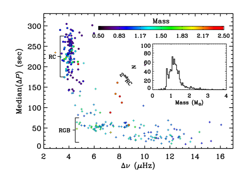
Figure 4.— Median period spacing versus $\Delta\nu$ for the 280 stars providing a clear classification into either red giant branch or red clump (including secondary clump). Dots show the helium core-burning stars, and stars show the red giant branch stars. The color of the symbols indicate the stellar mass derived from the $\Delta\nu$ and $\nu_{\mathrm{max}}$ scaling relations. The mass distribution of the plotted sample is shown in the inset.

Table 4Evolutionary stage and period spacing for 280 misclassified red giants

KIC	Median $\Delta P$ (s)	Evolutionary Stage
1160684	214.0	RC/2ndRC
1431059	16.3	RGB
2010577	190.9	RC/2ndRC
2014737	230.8	RC/2ndRC
2159728	60.4	RGB
2297384	230.5	RC/2ndRC
2297825	190.1	RC/2ndRC
2308968	276.4	RC/2ndRC
2436209	86.7	RGB
2436540	53.7	RGB
2437402	59.6	RGB
2437539	63.4	RGB
2437589	48.1	RGB
2437698	219.3	RC/2ndRC
2437805	179.6	RC/2ndRC
2438038	42.7	RGB
2570094	46.9	RGB
2708445	53.5	RGB
2850913	56.0	RGB
2865296	230.6	RC/2ndRC
3110892	260.0	RC/2ndRC
3239099	255.8	RC/2ndRC
3331116	231.7	RC/2ndRC
3432568	43.7	RGB
3534438	283.7	RC/2ndRC
3543446	23.2	RGB
3952678	238.2	RC/2ndRC
3953036	64.6	RGB
3956618	143.4	RC/2ndRC
3957962	244.4	RC/2ndRC
3964353	54.2	RGB
3965974	262.8	RC/2ndRC
3972205	47.3	RGB
3972697	266.5	RC/2ndRC
3974206	226.5	RC/2ndRC
4041075	194.5	RC/2ndRC
4041406	112.2	RC/2ndRC
4041741	50.5	RGB
4049147	90.7	RGB
4057657	257.8	RC/2ndRC
4067867	249.5	RC/2ndRC
4141587	200.1	RC/2ndRC
4141698	54.4	RGB
4246729	64.1	RGB
4248675	169.4	RC/2ndRC
4254250	239.8	RC/2ndRC
4254422	212.2	RC/2ndRC
4265786	12.1	RGB
4271799	278.8	RC/2ndRC
4366888	31.1	RGB
4446637	12.9	RGB
…

4. Discussion of the sample

4.1. Faint stars and distances

We looked at the distribution of some of the stellar properties of the misclassified red giant sample. Figure 5 shows the distribution of the Kepler magnitude for the confirmed red giants and for the $\sim$  13,000 public red giants in Huber et al. (2011). We clearly see that the new red giant sample is very different from the known red giants one: they are much fainter than the previously known sample.

Figure 5.— Comparison of the magnitude distribution of our confirmed red giants (bottom panel) and the public red giants (top panel).

Even though the stars are so faint, we are still able to detect solar-like oscillations and characterize their global properties. It seems from Figure 5 that Kepler would have been able to detect oscillations in giants even fainter than $Kp\,=\,16$ if they had been observed. This result is very promising for missions like K2 (Howell et al., 2014) and its galactic archeology program (Stello et al., 2015) and Transiting Exoplanet Survey Satellite (TESS Ricker et al., 2015).

Figure 6 shows the distance distribution of the newly classified red giants compared to another sample of red giants observed by Kepler. Rodrigues et al. (2014) determined the distances of $\sim$  2000 Kepler red giants that also had spectroscopic observations with the Apache Point Observatory Galactic Evolution Experiment (APOGEE Majewski et al., 2015). Their sample of stars (hereafter called the APOKASC sample) had distances up to $\sim$ 4 kpc. We note that the distances of the new red giants are quite large compared to the APOKASC sample and go well beyond 10 kpc. Our sample of new red giants has 404 stars at a distance larger than 5 kpc. This new sample allows us to probe our Galaxy further away and study stellar populations with seismology in a different region compared to what has been done so far with the CoRoT and Kepler missions. This can be seen in Figure 7, which is an update of the Figure 2 of Miglio et al. (2015).

We also computed the heights of the stars with respect to the Galactic plane to infer the possible number of halo stars present in our sample. Their position in the Galaxy are shown in the bottom panel of Figure 7. Figure 8 shows the distribution of the heights of the misclassified stars. We compared this distribution with a synthetic population of halo stars in the Kepler field with $J<16$ generated using Galaxia (Sharma et al., 2011), which shows that the majority of stars ($\gtrsim$60%) above 5 kpc are halo stars, while the faction of halo stars drops rapidly towards the galactic plane ($\lesssim$2% below 2 kpc). We divided the fraction of halo stars from the Galaxia model and our observed sample in height bins of 2 kpc to estimate the number of potential halo stars in each bin, yielding a total of about 40 red giants in our sample which could be halo stars. We note that this estimate is statistical only, and may be affected by systematic errors in the Galaxy model.

Figure 6.— Normalized distribution of the distances in parsec for the confirmed red giants of our sample (solid line) compared to the distances of the APOKASC red giants (dashed line) from Rodrigues et al. (2014).

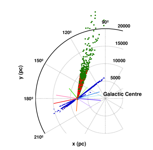
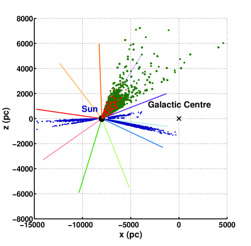
Figure 7.— Position in the Galaxy of the new red giants (green circles) compared to the stars in the CoRoT (blue dots), Kepler (red dots), and K2 fields (solid lines) as a function of x and y (top panel) and x and z (bottom panel).

Figure 8.— Distribution of the heights of the misclassified red giants.

4.2. Mass distribution of the sample

Figure 9 top panel presents the mass distribution of the newly classified red giants and the KASC sample of red giants (e.g. Huber et al., 2011) (red dashed line). Both samples peak at around 1.2 $M_{\odot}$. However, we clearly see that the number of high-mass (M larger than 1.3$M_{\odot}$) stars is smaller in our new sample compared to the KASC one as already noted in Section 3.4. There are slightly more stars with masses below 1.1 $M_{\odot}$. This agrees with the fact that these stars are more distant, and thus possibly halo stars. In the middle panel of Figure 9 we also note that the low-mass stars are in general fainter ($K_{p}>$14).

In fact, the generally lower mass of the sample would imply larger expected amplitudes at a given $\nu_{\rm max}$ (Stello et al., 2011). In Figure 1, we note that there are some stars with slightly higher mode amplitude ($A_{\rm max}$) compared to the general trend. We looked at the masses of the low-amplitude mode stars but did not find any systematic low-mass stars.

Given that some of these stars could belong to the halo and are thus metal-poor stars, some of the masses derived with the scaling relations should be taken cautiously. Indeed Epstein et al. (2014) studied a sample of halo stars observed by Kepler and showed that the scaling relations seem to deviate. As we do not have reliable metallicity measurement for these stars yet, we cannot take out the metal-poor stars from the sample.

We note that there are two stars (KIC 4850755 and 6266309) with a mass below 0.4M_⊙. Their parameters seem correct although KIC 4850755 seems a little odd from the visual inspection with a low number of modes observed and low amplitude for the l=1 modes as reported for example by García et al. (2014b) and theoretically explained by Fuller et al. (2015) and Stello et al. (2016). It could also be that scaling relations are not valid for such low-mass stars. More stars of this type would be needed to verify the validity of the scaling relations in this mass regime.

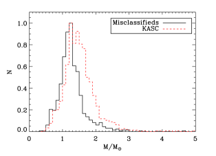
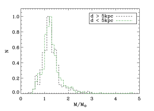
Figure 9.— Distribution of mass for the misclassified red giants. Top panel: mass histograms of our sample (black solid line) compared to the KASC sample (red dashed line). Middle panel: mass histograms for stars brighter (blue dotted-cached line) or fainter (black solid line) than a Kepler magnitude of 14. Bottom panel: mass histograms for stars in our sample which are closer than 5 kpc (red dashed-dotted line) and beyond 5 kpc (black dashed line).

We also looked at differences in the mass distribution as a function of distance (see bottom panel of Figure 9). We divided the sample into stars with distances larger than 5 kpc and stars with distances smaller than 5 kpc. The general distribution of both samples is very similar.

4.3. Possible explanations for dwarf classification

We checked the type of data and analysis that were used in the Kepler H14 catalog, to derive the effective temperature and the surface gravity of the 854 confirmed red giants. The majority of the stars of our sample have values obtained from the KIC. However, 24 stars have their $\log g$ determined by Huber et al. (2014) based on photometric observations and 8 stars were characterized by the work of Dressing & Charbonneau (2013) who analyzed optical and near-infrared photometry from the KIC to improve the stellar parameters of the cool Kepler dwarfs.

Recently, Gaidos et al. (2016) classified the cool Kepler dwarfs. We found six stars that overlap with our sample. They have the flag ’PM’ for ’Possible M dwarfs’. Four of them either a low crowding value or are possible pollution.

We aforementioned that the misclassified stars have their parameters determined from photometric observations. Distinguishing the luminosity class between dwarf and red giants can be a difficult task when only using multi-color photometry and the respective color indices. In approximately 4 % of KIC targets, there were significant discrepancies between different photometric temperature indicators (Pinsonneault et al., 2012). This fraction was comparable to the 3.8 % of targets with significant blends, estimated from a comparison of KIC photometry to that of the higher angular resolution SDSS photometry. In an even smaller minority of cases, the gravity classification was also in significant error, most likely due to a similar cause. Thus it is not surprising that 854 stars (less than 0.5% of the Kepler targets) were misclassified. This number of stars is actually remarkably low given the large number of targets.

4.4. Planet-Candidate Host Stars

Five of the newly classified red giants are planet-candidate hosts stars. In Table 5, we compare the new seismic stellar radius with the H14 value. Most of these stars were classified as M-dwarfs but now that they are classified as red giants, their new radii are 7 to 21 times larger than the ones listed in the H14 catalog.

We combined our revised stellar radii with the transit depths listed at the NASA Exoplanet Archive to re-calculate the planet-candidate radii, also given in Table 5. To calculate the uncertainties on the planet radius, we used a symmetric uncertainty on the ratio $R_{p}/R_{*}$ where we decided to take the largest values of the positive and negative values and then propagated the error bars. Given the new classification of the host stars, the estimated planet sizes have changed from Earth-size/superEarth-size planets to objects bigger than 5$\times R_{+}$.

To re-evaluate the planet-candidate status we used the revised stellar mass and radius to estimate the expected transit duration for a circular orbit and compared this to the observed transit durations. For three planet-candidate hosts (KOI-5652, KOI-5859, KOI-2813) the observed durations are significantly shorter than expected for a planet orbiting an evolved star, indicating that the planet-candidate would have to be either on a highly eccentric orbit or have an extremely high impact parameter. Inspection of the data validation (DV) reports showed that KOI-5652 and KOI-5859 both have low S/N, and hence are likely spurious detections due to the high correlated noise in giants due to stellar granulation. KOI-2813 is flagged as a likely false positive according to spectroscopic follow-up observations by the Kepler Community Follow-Up, which is supported by our reclassification of the host star. Finally, KOI-4902.01 and KOI-6217.01 show transit durations which are compatible with a low-luminosity RGB star, and hence remain viable planet-candidates.

Table 5Determination of the new planet radius for the planet-candidate host stars reclassified as red giants

KIC	KOI name	$R_{\rm p}/R_{\rm*}$	$R_{*}$ (new)	$R_{*}$ (old)	$R_{p}$ (new)	$R_{p}$ (old)	Planet-candidate
			($R_{\odot}$)	($R_{\odot}$)	($R_{+}$)	($R_{+}$)	status
9292100	K05652	0.021 $\pm$ 0.002	6.00 $\pm$ 0.44	0.63 $\pm$ 2.36	13.70 $\pm$ 2.08	1.43 $\pm$ 5.41	Likely FP
10000162	K04902	0.020 $\pm$ 0.003	5.44 $\pm$ 0.38	0.80 $\pm$ 0.26	12.10 $\pm$ 2.40	1.78 $\pm$ 0.57	PC
10200627	K06217	0.011 $\pm$ 0.001	4.23 $\pm$ 0.56	0.54 $\pm$ 0.04	5.01 $\pm$ 0.99	0.64 $\pm$ 0.04	PC
11100170	K05869	0.032 $\pm$ 0.002	11.90 $\pm$ 0.89	0.69 $\pm$ 0.07	41.65 $\pm$ 6.06	2.42 $\pm$ 0.23	Likely FP
11197853	K02813	0.011 $\pm$ 0.001	10.47 $\pm$ 0.75	0.62 $\pm$ 1.88	12.15 $\pm$ 1.75	0.73 $\pm$ 2.18	Likely FP

5. Conclusions

The analysis of 45,431 dwarfs from the Q1-Q16 Kepler star properties catalog (Huber et al., 2014) led to the re-classification of 854 of them as red giants, among which 31 stars have modes close to or above the Nyquist frequency. The comparison of the power spectra with known red giants and the inspection of UKIRT J-band images suggest that some of these newly classified red giants could still result from the presence of a nearby star.

We analyzed the light curves with two different pipelines, A2Z+ and SYD, and measured the global parameters of the acoustic modes. We then computed stellar fundamental parameters such as mass and radius from scaling relations and revised effective temperatures and distances from isochrone fitting for stars with modes below Nyquist frequency and for which colors were available. Among that sample of stars, we determined the evolutionary stage of 280 stars based on the period spacing of mixed modes.

We find that this sample of new red giants are less massive, fainter, and more distant than the previously known sample of red giants observed by Kepler, extending the parameter space. This work demonstrates that we can push the mode-detection limits in red giants to much fainter stars up to $Kp$ around 16.

These faint red giants represent a goldmine for galactic archeology studies (e.g. Miglio et al., 2013; Stello et al., 2015) as these stars probe the edge of the Milky Way. They will be observed by APOGEE in order to study their composition and have additional information to better understand the chemical evolution of the Galaxy.

Appendix A Comparison of the A2Z+ and SYD pipelines

A.1. Seismic parameters

The $\Delta\nu$ and $\nu_{\rm max}$ comparison for 748 stars is shown in Figure 10. For 97.7% of the stars, the agreement in $\Delta\nu$ is better than 1 $\sigma$. Concerning $\nu_{\rm max}$, both pipelines agree within 1 $\sigma$ for $\sim$ 98.7% of the stars. The relative difference in $\Delta\nu$ (resp. $\nu_{\rm max}$) is lower than 3% for 91% (resp. 85%) of the stars. The disagreement is larger in two regions: at very low frequency ($\mbox{$\nu_{\rm max}$}<10\mu$Hz and $\mbox{$\Delta\nu$}<2.5\mu$Hz) and around $\mbox{$\nu_{\rm max}$}\sim$ 30 $\mu$Hz and $\mbox{$\Delta\nu$}\sim$ 4 $\mu$Hz.

At very low frequency, due to limited resolution and the lower number of modes observed, it can be more difficult to fit a Gaussian to the excess power (method used by A2Z+ to estimate $\nu_{\rm max}$). Moreover, the computation of $\nu_{\rm max}$ is obtained after subtracting the background. As a consequence, if the background is fitted slightly differently by each method, it can affect the position of the maximum power. Moreover, in this frequency-range, the modes show stronger non-asymptotic behavior (Stello et al., 2014). So a slight difference in the number of orders taken to compute the mean large frequency separation and the frequency range can have an impact on the final estimate of $\Delta\nu$. We did a few tests with A2Z+ and found that in some cases it can lead to more than 3% change in $\Delta\nu$ for low $\nu_{\rm max}$.

The second frequency range where the largest disagreements are found corresponds to the clump stars where the mixed modes (resulting from the coupling between the p-mode and g-mode cavities) are clearly present, making the determination of $\Delta\nu$ more difficult to obtain.

There are 18 stars that disagree by more than 1 $\sigma$ in terms of $\Delta\nu$. For 11 of them the difference is of the order of a few 0.01$\mu$Hz. For the remaining 7 stars the SNR is too low to see if one value is better than the other. In terms of $\nu_{\rm max}$, ten stars disagree by more than 1$\sigma$ among which two (KIC 5351659 and 10587397) have a very low SNR. After visual inspection, for six stars (KIC 2422890, 4383163, 5976435, 9589159, 9712670, and 12599753) the A2Z+ value seems to be a better representation of $\nu_{\rm max}$ while for two stars (KIC 5036900 and 6525060) the SYD value seems to be closer to the observed $\nu_{\rm max}$.

Figure 10.— Difference in the mean large separation (left panel) and the frequency of maximum power (right panel) between the two pipelines A2Z+ and SYD as a function of the A2Z+ values (top panel) and in units of $\sigma$ computed as the quadratic sum of the uncertainties from A2Z+ and SYD (bottom panel).

We note that the uncertainties provided by the two pipelines are quite different. For $\nu_{\rm max}$, SYD has an average uncertainty of $\sim$2% and A2Z+ around 6%. For $\Delta\nu$, SYD has an average uncertainty of 0.6% compared to 3% for A2Z+. This difference is due to the different methods used. A2Z+ uncertainties are computed based on power centroids methods as described in Hekker et al. (2010), which is known to be quite conservative. The uncertainties of the SYD pipeline are computed through Monte-Carlo simulations by perturbing the power spectrum according to a $\chi^{2}$ distribution with two degrees of freedom, and repeating the $\nu_{\rm max}$ and $\Delta\nu$ measurements 500 times per star. The uncertainties are then estimated from the standard deviation of the resulting $\nu_{\rm max}$ and $\Delta\nu$ distributions.

A.2. Stellar fundamental parameters

As explained in Section 3.3, we computed the revised effective temperature of these stars by fitting isochrones and using constraints on the colors and the seismic parameters ($\Delta\nu$ and $\nu_{\rm max}$). Figure 11 represents the HR Diagram for the two pipelines with the revised effective temperature and the seismic $\log g$ from scaling relations. We can see that they look very similar even with slightly different seismic parameters.

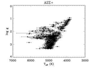
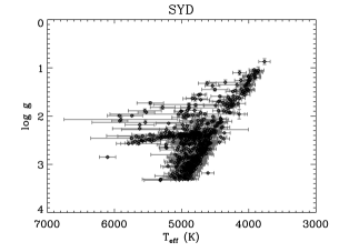
Figure 11.— HR Diagram obtained for the two pipelines where the effective temperature was computed with the isochrone fitting code (see Section 3.4) and the surface gravities were calculated from the scaling relations.

Figure 10 represents the comparison of the effective temperature and the distance for both pipelines. We note that the stellar parameters obtained from the isochrones fitting agree well within the uncertainties. Since the main contributors for the determination of the effective temperatures are the colors, the difference in the uncertainties on this parameter between A2Z+ and SYD is small. The seismic parameters have more impact on the distance derivation. We note that while the average uncertainty on $\Delta\nu$ (resp. $\nu_{\rm max}$) is five times (resp. three times) larger for A2Z+ compared to SYD the mean relative uncertainty on the distance is 1.6 times larger for A2Z+ than for SYD.

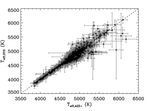
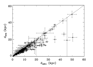
Figure 12.— Comparison of the effective temperature and distance obtained from the isochrone fitting code for the two pipelines. redo d in log scale

Finally, we compare the distribution in radius and mass computed with uncorrected scaling relations between A2Z+ and SYD in Figure 13. We can see that the distributions are quite similar and agree well within the uncertainties. Here we can note the difference in the uncertainties due to the larger uncertainties on the seismic parameters for the A2Z+ pipeline as explained in the previous section.

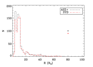
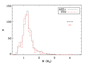
Figure 13.— Comparison of the radius and mass obtained from the scaling relation for the two pipelines. The error bars on the right hand-side represent the typical uncertainties of each method.

References

- Amôres & Lépine (2005) Amôres, E. B., & Lépine, J. R. D. 2005, AJ, 130, 659
- Batalha et al. (2010) Batalha, N. M., et al. 2010, ApJ, 713, L109
- Beck et al. (2011) Beck, P. G., et al. 2011, Science, 332, 205
- Bedding et al. (2011) Bedding, T. R., et al. 2011, Nature, 471, 608
- Bressan et al. (2012) Bressan, A., Marigo, P., Girardi, L., Salasnich, B., Dal Cero, C., Rubele, S., & Nanni, A. 2012, MNRAS, 427, 127
- Brown et al. (2011) Brown, T. M., Latham, D. W., Everett, M. E., & Esquerdo, G. A. 2011, AJ, 142, 112
- Bruntt et al. (2012) Bruntt, H., et al. 2012, MNRAS, 423, 122
- Casagrande et al. (2011) Casagrande, L., Schönrich, R., Asplund, M., Cassisi, S., Ramírez, I., Meléndez, J., Bensby, T., & Feltzing, S. 2011, A&A, 530, A138
- Chaplin et al. (2014) Chaplin, W. J., Elsworth, Y., Davies, G. R., Campante, T. L., Handberg, R., Miglio, A., & Basu, S. 2014, MNRAS, 445, 946
- Chaplin et al. (2011) Chaplin, W. J., et al. 2011, ApJ, 732, 54
- Dong et al. (2014) Dong, S., et al. 2014, ApJ, 789, L3
- Dressing & Charbonneau (2013) Dressing, C. D., & Charbonneau, D. 2013, ApJ, 767, 95
- Dupret et al. (2009) Dupret, M.-A., et al. 2009, A&A, 506, 57
- Epstein et al. (2014) Epstein, C. R., et al. 2014, ApJ, 785, L28
- Fuller et al. (2015) Fuller, J., Cantiello, M., Stello, D., Garcia, R. A., & Bildsten, L. 2015, Science, 350, 423
- Gaidos et al. (2016) Gaidos, E., Mann, A. W., Kraus, A. L., & Ireland, M. 2016, MNRAS, 457, 2877
- García et al. (2011) García, R. A., et al. 2011, MNRAS, 414, L6
- García et al. (2014a) —. 2014a, A&A, 568, A10
- García et al. (2014b) —. 2014b, A&A, 563, A84
- Hekker et al. (2010) Hekker, S., et al. 2010, MNRAS, 402, 2049
- Holtzman et al. (2015) Holtzman, J. A., et al. 2015, AJ, 150, 148
- Howell et al. (2014) Howell, S. B., et al. 2014, PASP, 126, 398
- Huber et al. (2009) Huber, D., Stello, D., Bedding, T. R., Chaplin, W. J., Arentoft, T., Quirion, P., & Kjeldsen, H. 2009, Communications in Asteroseismology, 160, 74
- Huber et al. (2011) Huber, D., et al. 2011, ApJ, 743, 143
- Huber et al. (2013) —. 2013, ApJ, 767, 127
- Huber et al. (2014) —. 2014, ApJS, 211, 2
- Jenkins et al. (2010) Jenkins, J. M., et al. 2010, ApJ, 713, L87
- Kallinger et al. (2014) Kallinger, T., et al. 2014, A&A, 570, A41
- Kjeldsen & Bedding (1995) Kjeldsen, H., & Bedding, T. R. 1995, A&A, 293, 87
- Majewski et al. (2015) Majewski, S. R., et al. 2015, ArXiv e-prints
- Mann et al. (2012) Mann, A. W., Gaidos, E., Lépine, S., & Hilton, E. J. 2012, ApJ, 753, 90
- Mathur et al. (2010) Mathur, S., et al. 2010, A&A, 511, A46
- Mathur et al. (2011) —. 2011, ApJ, 741, 119
- Miglio et al. (2015) Miglio, A., Girardi, L., Rodrigues, T. S., Stello, D., & Chaplin, W. J. 2015, Astrophysics and Space Science Proceedings, 39, 11
- Miglio et al. (2013) Miglio, A., et al. 2013, MNRAS, 429, 423
- Mosser & Appourchaux (2009) Mosser, B., & Appourchaux, T. 2009, ArXiv 0909.0782
- Mosser et al. (2012) Mosser, B., et al. 2012, A&A, 540, A143
- Mosser et al. (2014) —. 2014, A&A, 572, L5
- Pinsonneault et al. (2012) Pinsonneault, M. H., An, D., Molenda-Żakowicz, J., Chaplin, W. J., Metcalfe, T. S., & Bruntt, H. 2012, ApJS, 199, 30
- Pires et al. (2015) Pires, S., Mathur, S., García, R. A., Ballot, J., Stello, D., & Sato, K. 2015, A&A, 574, A18
- Ricker et al. (2015) Ricker, G. R., et al. 2015, Journal of Astronomical Telescopes, Instruments, and Systems, 1, 014003
- Rodrigues et al. (2014) Rodrigues, T. S., et al. 2014, MNRAS, 445, 2758
- Serenelli et al. (2013) Serenelli, A. M., Bergemann, M., Ruchti, G., & Casagrande, L. 2013, MNRAS, 429, 3645
- Sharma et al. (2011) Sharma, S., Bland-Hawthorn, J., Johnston, K. V., & Binney, J. 2011, ApJ, 730, 3
- Stello et al. (2016) Stello, D., Cantiello, M., Fuller, J., Huber, D., García, R. A., Bedding, T. R., Bildsten, L., & Silva Aguirre, V. 2016, Nature, 529, 364
- Stello et al. (2009) Stello, D., Chaplin, W. J., Basu, S., Elsworth, Y., & Bedding, T. R. 2009, MNRAS, 400, L80
- Stello et al. (2011) Stello, D., et al. 2011, ApJ, 737, L10
- Stello et al. (2013) —. 2013, ApJ, 765, L41
- Stello et al. (2014) —. 2014, ApJ, 788, L10
- Stello et al. (2015) —. 2015, ApJ, 809, L3
- Thygesen et al. (2012) Thygesen, A. O., et al. 2012, A&A, 543, A160
- Verner et al. (2011) Verner, G. A., et al. 2011, ApJ, 738, L28