Edit distance and its computation

Abstract

In this paper, we provide a method for determining the asymptotic value of the maximum edit distance from a given hereditary property. This method permits the edit distance to be computed without using Szemerédi’s Regularity Lemma directly.

Using this new method, we are able to compute the edit distance from hereditary properties for which it was previously unknown. For some graphs $H$, the edit distance from ${\rm Forb}(H)$ is computed, where ${\rm Forb}(H)$ is the class of graphs which contain no induced copy of graph $H$.

Those graphs for which we determine the edit distance asymptotically are $H=K_{a}+E_{b}$, an $a$-clique with $b$ isolated vertices, and $H=K_{3,3}$, a complete bipartite graph. We also provide a graph, the first such construction, for which the edit distance cannot be determined just by considering partitions of the vertex set into cliques and cocliques.

In the process, we develop weighted generalizations of Turán’s theorem, which may be of independent interest.

1 Introduction

Throughout this paper, we use standard terminology in the theory of graphs. See, for example, [6]. A subgraph devoid of edges, usually called an independent set, is referred to in this paper as a coclique, so that it parallels the notion of a clique.

1.1 Background

The edit distance of graphs was defined in [4] as follows:

Definition 1

Let ${\cal P}$ denote a class of graphs. If $G$ is a fixed graph, then the edit distance from $G$ to ${\cal P}$ is

$${\rm Dist}(G,{\cal P})=\min\left\{\left|E(F)\triangle E(G)\right|:F\in{\cal P},V(F)=V(G)\right\}$$

and the edit distance from $n$-vertex graphs to ${\cal P}$ is

$${\rm Dist}(n,{\cal P})=\max\left\{{\rm Dist}(G,{\cal P}):|V(G)|=n\right\}.$$

It is natural to consider hereditary properties of graphs. A hereditary property is one that is closed under the deletion of vertices. In fact, edge-modification for such properties is an important question in computer science, as described in Alon and Stav [1] and biology, as shown in [4].

Clearly, ${\rm Forb}(H)$ is a hereditary property for any graph $H$. In fact, every hereditary property, ${\cal H}$, can be expressed as $\bigcap_{H\in{\cal F}({\cal H})}{\rm Forb}(H)$, where the intersection is over the family ${\cal F}({\cal H})$, which consists of all graphs $H$ which are the minimal elements of $\overline{{\cal H}}$.

In [1], Alon and Stav prove that, for every hereditary property ${\cal H}$, there exists a $p^{*}=p^{*}({\cal H})$ such that, with high probability, ${\rm Dist}(n,{\cal H})={\rm Dist}\left(G(n,p^{*}),{\cal H}\right)+o(n^{2})$, where $G(n,p)$ denotes the usual Erdős-Rényi random graph. This fact can be used to prove the existence of

$$d^{*}({\cal H})\stackrel{{\scriptstyle\rm def}}{{=}}\lim_{n\rightarrow\infty}{\rm Dist}(n,{\cal H})/\binom{n}{2}.$$

1.2 Previous results

The previously-known general bounds for ${\rm Dist}(n,{\rm Forb}(H))$ are expressed in terms of the so-called binary chromatic number:

Definition 2

The binary chromatic number of a graph $G$, $\chi_{B}(G)$ is the least integer $k+1$ such that, for all $c\in\{0,\ldots,k+1\}$, there exists a partition of $V(G)$ into $c$ cliques and $k+1-c$ cocliques.

The binary chromatic number [4] is called the “colouring number” of a hereditary property by Bollobás and Thomason [9] and again by Bollobás [5] and is called the parameter $\tau(H)$ in Prömel and Steger [21]. The term indicates its generalizibility to multicolorings of the edges of $K_{n}$, or $K_{n,n}$ as in [3].

The binary chromatic number gives the value of ${\rm Dist}(n,{\rm Forb}(H))$ to within a multiplicative factor of $2$, asymptotically:

Theorem 3 ([4])

If $H$ is a graph with binary chromatic number $\chi_{B}(H)=k+1$, then $\left(\frac{1}{2k}-o(1)\right)\binom{n}{2}\leq{\rm Dist}\left(n,{\rm Forb}(H)\right)\leq\frac{1}{k}\binom{n}{2}$.

1.2.1 Known values of $d^{*}$ and $p^{*}$

In [4], a large class of graphs $H$ for which $d^{*}({\rm Forb}(H))$ is known to be the lower bound in Theorem 3 is described. Namely, if a graph $H$ has the property that $\chi_{B}(H)=k+1$ and there exist $(A,c)$ and $(a,C)$ such that each of the following occurs

• $V(H)$ cannot be partitioned into $c$ cliques and $A$ cocliques,

• $V(H)$ cannot be partitioned into $C$ cliques and $a$ cocliques,

• $A+c=a+C=k$ and $c\leq k/2\leq C$,

then

$$d^{*}({\rm Forb}(H))=\frac{1}{2k}.$$

It is observed in [1] that if $H$ and $(A,c)$ and $(a,C)$ satisfy the conditions above, then $p^{*}({\rm Forb}(H))=1/2$. Furthermore, if $H$ is a self-complementary graph, then $A=C$ and $a=c$. So, $C+c=k$, which implies $c\leq k/2\leq C$ and $\left(p^{*}({\rm Forb}(H)),d^{*}({\rm Forb}(H))\right)=\left(1/2,1/(2k)\right)$.

The edit distance from monotone properties is also well-known. A monotone property is, without loss of generality, closed under the removal of either vertices or edges. Let ${\cal M}$ be a monotone property of graphs. The theorems of Erdős and Stone [15] and Erdős and Simonovits [14] give that

$$d^{*}({\cal M})=1/r,\qquad\mbox{where }r=\min\{\chi(F)-1:F\not\in{\cal M}\}\qquad\text{and}\qquad p^{*}({\cal M})=1.$$

Alon and Stav, in [2], prove that $d^{*}({\rm Forb}(K_{1,3}))=p^{*}({\rm Forb}(K_{1,3}))=1/3.$ In this paper, we generalize this result to compute the pairs $(p^{*},d^{*})$ for hereditary properties of the form ${\rm Forb}(K_{a}+E_{b})$ and ${\rm Forb}\left(\overline{K_{a}+E_{b}}\right)$, where $K_{a}$ is a complete graph on $a$ vertices, $E_{b}$ is an empty graph on $b$ vertices and the “$+$” denotes a disjoint union of graphs. The claw $K_{1,3}$ is $\overline{K_{3}+E_{1}}$.

In both [4] and in [2], more precise results for determining ${\rm Dist}(n,{\cal H})$ are given for several families of hereditary properties. For this paper, we concern ourselves exclusively with the first-order asymptotics.

Finally, in [2], a formula is given for the asymptotic value of the distance ${\rm Dist}(G(n,1/2),{\cal H})$ for an arbitrary hereditary property ${\cal H}$. It generalizes the result, stated in [1] and implicit from arguments in [4], that almost surely, ${\rm Dist}(G(n,1/2),{\rm Forb}(H))=\frac{1}{2(\chi_{B}({\rm Forb}(H))-1)}\binom{n}{2}-o(n^{2})$. In this paper, we will further generalize this by determining an asymptotic expression for ${\rm Dist}(G(n,p),{\cal H})$ for all $p\in[0,1]$.

1.3 Colored homomorphisms

Next we recall three definitions from [1] which are convenient for us.

Definition 4

A colored regularity graph (CRG), $K$, is a complete graph for which the vertices are partitioned $V(K)={\rm VW}(K)\mathbin{\ooalign{$\cup$\crcr\hfil\raise 8.0pt\hbox{\xviiroman.}\hfil\crcr}}{\rm VB}(K)$ and the edges are partitioned $E(K)={\rm EW}(K)\mathbin{\ooalign{$\cup$\crcr\hfil\raise 8.0pt\hbox{\xviiroman.}\hfil\crcr}}{\rm EG}(K)\mathbin{\ooalign{$\cup$\crcr\hfil\raise 8.0pt\hbox{\xviiroman.}\hfil\crcr}}{\rm EB}(K)$. The sets ${\rm VW}$ and ${\rm VB}$ are the white and black vertices, respectively, and the sets ${\rm EW}$, ${\rm EG}$ and ${\rm EB}$ are the white, gray and black edges, respectively.

Bollobás and Thomason ([8],[10]) originate the use of this structure to define so-called basic hereditary properties. In particular, the paper [10] generalizes the enumeration of graphs with a given property $\cal P$ to the problem of computing the probability that $G(n,p)\in{\cal P}$. The problems are equivalent if $p=1/2$. The papers use many of the techniques that are repeated or cited in the subsequent works on edit distance and use other nontrivial ideas.

Definition 5

Let $K$ be a CRG with $V(K)=\{v_{1},\ldots,v_{k}\}$. The graph property ${\cal P}_{K,n}$ consists of all graphs $J$ on $n$ vertices for which there is an equipartition ${\bf A}=\{A_{i}:1\leq i\leq k\}$ of the vertices of $J$ satisfying the following conditions for $1\leq i<j\leq k$:

• if $v_{i}\in{\rm VW}(K)$, then $A_{i}$ spans an empty graph in $J$,

• if $v_{i}\in{\rm VB}(K)$, then $A_{i}$ spans a complete graph in $J$,

• if $\{v_{i},v_{j}\}\in{\rm EW}(K)$, then $(A_{i},A_{j})$ spans an empty bipartite graph in $J$,

• if $\{v_{i},v_{j}\}\in{\rm EB}(K)$, then $(A_{i},A_{j})$ spans a complete bipartite graph in $J$,

• if $\{v_{i},v_{j}\}\in{\rm EG}(K)$, then $(A_{i},A_{j})$ is unrestricted.

If all of the above holds, we say that the equipartition witnesses the membership of $J$ in ${\cal P}_{K,n}$.

Definition 6

A colored-homomorphism from a (simple) graph $F$ to a CRG, $K$, is a mapping $\varphi:V(F)\rightarrow V(K)$, which satisfies the following:

1. If $\{u,v\}\in E(F)$ then either $\varphi(u)=\varphi(v)=t\in{\rm VB}(K)$, or $\varphi(u)\neq\varphi(v)$ and $\left\{\varphi(u),\varphi(v)\right\}\in{\rm EB}(K)\cup{\rm EG}(K)$.

2. If $\{u,v\}\not\in E(F)$ then either $\varphi(u)=\varphi(v)=t\in{\rm VW}(K)$, or $\varphi(u)\neq\varphi(v)$ and $\left\{\varphi(u),\varphi(v)\right\}\in{\rm EW}(K)\cup{\rm EG}(K)$.

Moreover, a colored-homomorphism can be defined from a CRG, $K^{\prime}$, to another CRG, $K^{\prime\prime}$, that satisfies the following:

1. If $v\in{\rm VB}(K^{\prime})$, then $\varphi(v)\in{\rm VB}(K^{\prime\prime})$. If $v\in{\rm VW}(K^{\prime})$, then $\varphi(v)\in{\rm VW}(K^{\prime\prime})$.

2. If $(u,v)\in{\rm EB}(K^{\prime})$ then either $\varphi(u)=\varphi(v)=t\in{\rm VB}(K^{\prime\prime})$, or $\varphi(u)\neq\varphi(v)$ and $\left(\varphi(u),\varphi(v)\right)\in{\rm EB}(K^{\prime\prime})\cup{\rm EG}(K^{\prime\prime})$.

3. If $(u,v)\in{\rm EW}(K^{\prime})$ then either $\varphi(u)=\varphi(v)=t\in{\rm VW}(K^{\prime\prime})$, or $\varphi(u)\neq\varphi(v)$ and $\left(\varphi(u),\varphi(v)\right)\in{\rm EW}(K^{\prime\prime})\cup{\rm EG}(K^{\prime\prime})$.

Note that we can use the second definition to include the first, by defining $V(F)={\rm VW}(F)\mathbin{\ooalign{$\cup$\crcr\hfil\raise 8.0pt\hbox{\xviiroman.}\hfil\crcr}}{\rm VB}(F)$ in such a way as to make the colored-homomorphism legal with respect to the edge set.

Definition 7

A CRG, $K^{\prime}$, is induced in another CRG, $K$, if there is a colored-homomor-phism $\varphi:V(K^{\prime})\rightarrow V(K)$ such that

• $\varphi$ is an injection and

• for any $u,v\in V(K^{\prime})$ for which $\left\{\varphi(u),\varphi(v)\right\}\in{\rm EG}(K)$, then $\{u,v\}\in{\rm EG}(K^{\prime})$.

Definition 8

A CRG, $K$, is an ${\cal H}$-colored regularity graph (${\cal H}$-CRG) for a hereditary property ${\cal H}$ if, for every graph $J\not\in{\cal H}$, there is no colored-homomorphism from $J$ to $K$.

Denote ${\cal K}({\cal H})$ to be the family of all CRGs $K$ such that for every graph $J\not\in{\cal H}$ there is no colored-homomorphism from $J$ to $K$. If there is no colored-homomorphism from $J$ to $K$, then this is denoted as $J\not\mapsto_{c}K$. If there is a colored-homomorphism from $J$ to $K$, then this is denoted as $J\mapsto_{c}K$.

Observe that if ${\cal H}=\bigcap_{H\in{\cal F}({\cal H})}{\rm Forb}(H)$, then an ${\cal H}$-CRG, $K$, is one such that for all $H\in{\cal F}({\cal H})$, there is no colored-homomorphism from $H$ into $K$.

1.4 Functions of colored regularity graphs

1.4.1 Binary chromatic number

Previous edit distance results were expressed in terms of the so-called binary chromatic number, which can be viewed as an invariant on CRGs for which the edge set is gray.

Definition 9

Let $K(a,c)$ denote the CRG with $a$ white vertices, $c$ black vertices and all edges gray.

The binary chromatic number of a hereditary property ${\cal H}$, denoted $\chi_{B}({\cal H})$, is the least integer $k+1$ such that, $K(a,c)\not\in{\cal K}({\cal H})$ for all $a,c$ such that $a+c=k+1$. This definition means that $\chi_{B}({\rm Forb}(H))=\chi_{B}(H)$ for any graph $H$.

This quantity is too specific for our purposes. We need to introduce a function that accounts for nongray edges in CRGs.

1.4.2 The function $f$

Given a CRG, $K$, we define two functions. If $K$ has $k$ vertices, with the usual notation for the edge sets and the vertex sets, then let

$$f_{K}(p)\stackrel{{\scriptstyle\rm def}}{{=}}\frac{1}{k^{2}}\left[p\left(|{\rm VW}(K)|+2|{\rm EW}(K)|\right)+(1-p)\left(|{\rm VB}(K)|+2|{\rm EB}(K)|\right)\right].$$

The function that defines $f_{K}(p)$ was introduced in [1] and corresponds to equipartitioning the vertex set of some $G$ which is chosen according to the distribution $G(n,p)$ and mapping the parts of the partition to the vertices of $K$. So, $f$ represents the expected proportion of edges that are changed under the rule that if an edge is mapped to a white edge or its endvertices are mapped to the same white vertex, then the edge is removed and if a nonedge is mapped to a black edge or its endvertices are mapped to the same black vertex, then the edge is added.

The function $f_{K}(p)$, as a function of $p$, is a line with a slope in $[-1,1]$.

1.4.3 The function $g$

The function $g_{K}(p)$ is defined by a quadratic program. It corresponds not necessarily to an equipartition, but a partition with optimal sizes.

In order to define $g$, we first define some matrices: Let ${\bf W}_{K}$ denote the adjacency matrix of the graph defined by the white edges, along with the first $|{\rm VW}(K)|$ diagonal entries being $1$ (corresponding to the white vertices) and the other diagonal entries being $0$. Let ${\bf B}_{K}$ denote the adjacency matrix of the graph defined by the black edges along with the last $|{\rm VB}(K)|$ diagonal entries being $1$ (corresponding to the black vertices) and the other diagonal entries being $0$. We define the matrix ${\bf M}_{K}(p)$ as follows:

$${\bf M}_{K}(p)=p{\bf W}_{K}+(1-p){\bf B}_{K}.$$

With this, we define $g_{K}(p)$:

$$g_{K}(p):=\left\{\begin{array}[]{rlcl}\min&\lx@intercol{\bf u}^{T}{\bf M}_{K}(p){\bf u}\hfil\lx@intercol\\ {\rm s.t.}&{\bf u}^{T}{\bf 1}&=&1\\ &{\bf u}&\geq&{\bf 0}.\end{array}\right.$$ (1)

If an optimal solution ${\bf u}^{\prime}$ has zero entries, then $g_{K}(p)=g_{K^{*}}(p)$ for the CRG, $K^{*}$, induced in $K$, whose vertices correspond to the nonzero entries of ${\bf u}^{\prime}$. (Note that $K^{*}$ may depend on ${\bf u}^{\prime}$.)

Lemma 10

For any CRG $K$, and any $p\in[0,1]$, there exists a CRG $K^{*}$, where $K^{*}$ is defined as a CRG induced in $K$ by the vertices which correspond to nonzero entries of ${\bf u}^{\prime}$, such that $g_{K}(p)=g_{K^{*}}(p)=\frac{1}{{\bf 1}^{T}{\bf M}_{K^{*}}^{-1}(p){\bf 1}}$.

We prove Lemma 10 in Section 3.2.

2 Results

2.1 General bounds

Theorem 11 is our main theorem, relating the functions $f$ and $g$. For $p\in(0,1)$, the notation $G(n,p)$ is the random variable that represents a graph on $n$ vertices chosen by a random process in which each edge is present independently with probability $p$. For $m\geq 1$, $G(n,m)$ is the random variable that represents a graph on $n$ vertices chosen uniformly at random from all $n$ vertex graphs with $\lfloor m\rfloor$ edges.

Theorem 11

For a hereditary property ${\cal H}=\bigcap_{H\in{\cal F}({\cal H})}{\rm Forb}(H)$, let ${\cal K}({\cal H})$ denote all CRGs $K$ such that $H\not\mapsto_{c}K$ for each $H\in{\cal F}({\cal H})$. Then, $d^{*}({\cal H})\stackrel{{\scriptstyle\rm def}}{{=}}\lim_{n\rightarrow\infty}{\rm Dist}(n,{\cal H})/\binom{n}{2}$ exists. Define

$$f(p)\stackrel{{\scriptstyle\rm def}}{{=}}\inf_{K\in{\cal K}({\cal H})}f_{K}(p)\qquad\mbox{and}\qquad g(p)\stackrel{{\scriptstyle\rm def}}{{=}}\inf_{K\in{\cal K}({\cal H})}g_{K}(p).$$

Then it is the case that $f(p)=g(p)$ for all $p\in[0,1]$,

$$d^{*}({\cal H})=\max_{p\in[0,1]}f(p)=\max_{p\in[0,1]}g(p),$$

and $p^{*}({\cal H})$ is the value of $p$ at which $f$ achieves its maximum. In addition, the function $f(p)=g(p)$ is concave.

Furthermore, for all $p\in(0,1)$,

$$\max_{G:e(G)=p{\scriptstyle\binom{n}{2}}}\left\{{\rm Dist}(G,{\cal H})\right\}=f(p)\binom{n}{2}+o(n^{2}),$$

and for all $\epsilon>0$, ${\rm Dist}\left(G\left(n,p{\scriptstyle\binom{n}{2}}\right),{\cal H}\right)\geq f(p)\binom{n}{2}-\epsilon n^{2}$, with probability approaching 1 as $n\rightarrow\infty$.

Of course, by definition, ${\rm Dist}(n,{\rm Forb}({\cal H}))=d^{*}({\cal H})\binom{n}{2}+o(n^{2})$.

Remark: The main theorem of Alon and Stav [1] states, informally, that there exists a $p^{*}=p^{*}({\cal H})$ such that ${\rm Dist}(n,{\cal H})={\rm Dist}(G(n,p^{*}),{\cal H})$. Here, we compute the first-order asymptotic of the edit distance and show that $f(p)\binom{n}{2}$ is asymptotically the maximum edit distance among all graphs of density $p$, and is achieved by the random graph $G(n,p{\scriptstyle\binom{n}{2}})$. Informally, ${\rm Dist}\left(G(n,p{\scriptstyle\binom{n}{2}}),{\cal H}\right)=f(p)\binom{n}{2}+o(n^{2})$ and in the proof, we show, that ${\rm Dist}\left(G(n,p),{\cal H}\right)=f(p)\binom{n}{2}+o(n^{2})$ as well.

In addition, Theorem 11 has the advantage that the edit distance can be computed, asymptotically, without direct use of Szemerédi’s Regularity Lemma. As we see in Theorems 12, 13, 14 and 15, the function $f(p)$ is very useful in computing the values of $\left(p^{*}({\cal H}),d^{*}({\cal H})\right)$.

The method for computing $(p^{*},d^{*})$ in this paper follows the same pattern for every hereditary property.

Method for computing edit distance:
Upper bound: Carefully choose CRGs, $K^{\prime},K^{\prime\prime}\in{\cal K}({\cal H})$ (possibly $K^{\prime}=K^{\prime\prime}$) and compute $\max_{p\in[0,1]}\min\left\{g_{K^{\prime}}(p),g_{K^{\prime\prime}}(p)\right\}$. This maximum is an upper bound for $d^{*}({\cal H})$.

Lower bound: Let $p^{*}$ be the value of $p$ at which the function $\min\left\{g_{K^{\prime}}(p),g_{K^{\prime\prime}}(p)\right\}$ achieves its maximum. For any $K\in{\cal K}({\cal H})$, we try to show that $f_{K}(p^{*})$ is at least the upper bound value. If this is the case, then we have computed $d^{*}({\cal H})$; moreover, $p^{*}({\cal H})$ is the $p^{*}$ provided above. In order to do this, we use a type of weighted Turán theorem.

2.2 The edit distance of $K_{a}+E_{b}$

We give a class of graphs in which neither the upper nor the lower bounds given by the binary chromatic number hold.

Theorem 12

Let $a\geq 2$ and $b\geq 1$ be positive integers. Let $H=K_{a}+E_{b}$, the disjoint union of an $a$-clique and a $b$-coclique. Then,

$$d^{*}\left({\rm Forb}(K_{a}+E_{b})\right)=\frac{1}{a+b-1}\quad\text{ and }\quad p^{*}\left({\rm Forb}(K_{a}+E_{b})\right)=\frac{a-1}{a+b-1},$$

i.e., ${\rm Dist}(n,{\rm Forb}(K_{a}\cup E_{b}))=\frac{1}{a+b-1}\binom{n}{2}-o(n^{2})$.

We note that $\chi_{B}(K_{a}+E_{b})=\max\{a,b+1\}$ and so Theorem 12 is an improvement over [4] in the case when $a\neq b+1$. It is also an improvement over Proposition 17, which appears below, in the case when $b>1$ and $a>2$. Alon and Stav [2] prove the case when $a=3$ and $b=1$, the complement of the “claw,” $K_{1,3}$.

2.3 A few specific graphs

In all known examples of hereditary properties ${\cal H}$, the point at which $\left(p^{*}({\cal H}),d^{*}({\cal H})\right)$ occurs is either the intersection of two curves $g_{K^{\prime}}(p)$, $g_{K^{\prime\prime}}(p)$ or is the maximum of a single curve $g_{K^{\prime}}(p)$. In either case, each CRG can be chosen to be one with only gray edges.

We compute the edit distance of two hereditary properties that demonstrate the complexity of both $p^{*}$ and $d^{*}$.

2.3.1 The graph $K_{3,3}$

The graph $K_{3,3}$ has $d^{*}$ and $p^{*}$ defined by the local maximum of a single curve $g_{K^{\prime}}(p)$.

Theorem 13

The complete bipartite graph $K_{3,3}$ satisfies

$$p^{*}\left({\rm Forb}(K_{3,3})\right)=\sqrt{2}-1\quad\text{and}\quad d^{*}\left({\rm Forb}(K_{3,3})\right)=3-2\sqrt{2}.$$

Moreover, $p^{*}$ is the local maximum of $g_{K^{\prime}}(p)$, where $K^{\prime}$ consists of one white vertex, two black vertices and all gray edges.

It should be noted that neither $p^{*}$ nor $d^{*}$ could be determined for this hereditary property by the intersection of a finite number of $f$ curves, simply because such intersections would occur at rational points. So, a sequence of CRGs would be required. By using the $g$ curves, however, we need only to use a single CRG.

2.3.2 The graph $H_{9}$

Here, the graph we construct is formed by taking $C_{9}^{2}$ and adding a triangle. That is, if the vertices are $\{0,1,2,3,4,5,6,7,8\}$, then $i\sim j$ iff $i-j\in\{\pm 1,\pm 2\}\pmod{9}$ or both $i$ and $j$ are congruent to 0 modulo $3$. For notational simplicity, we call this graph $H_{9}$. See Figure 1.

Figure 1: The graph $H_{9}$.

An upper bound on $d^{*}({\rm Forb}(H_{9}))$ is defined by the intersection of two curves, $g_{K^{\prime}}(p)$, $g_{K^{\prime\prime}}(p)$, one of which corresponds to a CRG that has one black edge. For this graph $H_{9}$, it is impossible to only consider CRGs which have all edges gray. It was a folklore belief that for every graph it is sufficient to consider CRGs which have all edges gray, $H_{9}$ is the first example showing that this belief is false.

Theorem 14

The graph $H_{9}$ satisfies

$$d^{*}\left({\rm Forb}(H_{9})\right)\leq\frac{3-\sqrt{5}}{4}.$$

Moreover, this value occurs at the intersection of $g_{K^{\prime}}(p)$ and $g_{K^{\prime\prime}}(p)$, where $K^{\prime}$ consists of two black vertices and a gray edge and $K^{\prime\prime}$ consists of four white vertices, a black edge and 5 gray edges.

In the proof, we show that if only gray-edge CRGs are used, then the upper bound on $d^{*}$ could be no less than $1/5=0.2$, but $\frac{3-\sqrt{5}}{4}\approx 0.191$. The lower bound, from Theorem 3, is $d^{*}({\rm Forb}(H_{9}))\geq 1/6\approx 0.167$.

2.4 4-vertex graphs

In [2], Alon and Stav compute $\left(p^{*}({\rm Forb}(H)),d^{*}({\rm Forb}(H))\right)$ for all $H$ on at most 4 vertices. Except for $P_{3}+K_{1}$ and its complement, all such graphs $H$ are either covered by Theorem 16 (see also [4]) or are of the form $K_{a}+E_{b}$ or $\overline{K_{a}+E_{b}}$, which is covered by Theorem 12. Here we give a short and different proof, using Lemma 18, for $\overline{P_{3}+K_{1}}$, which consists of a triangle and a pendant edge.

Theorem 15

The graph $\overline{P_{3}+K_{1}}$ satisfies

$$p^{*}\left({\rm Forb}(\overline{P_{3}+K_{1}})\right)=2/3\qquad\mbox{and}\qquad d^{*}\left({\rm Forb}(\overline{P_{3}+K_{1}})\right)=1/3.$$

3 Basic tools

3.1 Improved binary chromatic number bounds

Lemma 10, along with Theorem 11, yields a proof of a somewhat better upper bound for ${\rm Dist}(n,{\cal H})$, based on the binary chromatic number.

Recall that $K(a,c)$ denotes the CRG that consists of $a$ white vertices, $c$ black vertices and only gray edges. If $k=\chi_{B}({\cal H})-1$, then let $c_{\rm min}$ be the least $c$ so that $K(k-c,c)\not\in{\cal K}({\cal H})$. Let $c_{\rm max}$ be the greatest such number. For ${\cal H}={\rm Forb}(H)$, there exists an upper bound that can be expressed in terms of the binary chromatic number of $H$ and corresponding $c_{\rm min}$ and $c_{\rm max}$.

Theorem 16 ([4])

Let $H$ be a graph with binary chromatic number $k+1$ and $c_{\rm min}$ and $c_{\rm max}$ be defined as above. If $c_{\rm min}\leq k/2\leq c_{\rm max}$, then

$$d^{*}({\rm Forb}(H))=\frac{1}{2k}.$$

Otherwise, let $c_{0}$ be the one of $\{c_{\rm max},c_{\rm min}\}$ that is closest to $k/2$. Then

$$d^{*}({\rm Forb}(H))\leq\left(\frac{1}{1+2\sqrt{\frac{c_{0}}{k}\left(1-\frac{c_{0}}{k}\right)}}\right)\frac{1}{k}\leq\frac{1}{k}.$$

Proposition 17 improves this general upper bound, not only trivially by extending it to general hereditary properties, but also by improving the case when $c_{\rm max}=0$ or $c_{\rm min}=k$.

Proposition 17

Let ${\cal H}$ be a hereditary property with $k+1=\chi_{B}({\cal H})$ and $c_{0},c_{\rm max},c_{\rm min}$ defined analogously to Theorem 16. The bounds in Theorem 16 hold for ${\cal H}$. Furthermore, if ${\cal H}\neq{\rm Forb}(K_{k+1})$, then

$$d^{*}({\cal H})\leq\frac{1}{k+1}.$$

Note that $d^{*}({\rm Forb}(K_{k+1}))=\frac{1}{k}$ by Turán’s theorem.

Proof.  If we restrict our attention to the CRGs in ${\cal K}({\cal H})$ which are of the form $K(a,c)$, then Theorem 11 gives that

$$d^{*}({\cal H})\leq\max_{p\in[0,1]}\inf_{K(a,c)\in{\cal K}({\cal H})}\left\{g_{K(a,c)}(p)\right\}=\max_{p\in[0,1]}\min_{K(a,c)\in{\cal K}({\cal H})}\left\{\frac{p(1-p)}{a(1-p)+cp}\right\}.$$

A word on why the “$\inf$” is made into a “$\min$”: Recall that if ${\cal H}=\bigcap_{H\in{\cal F}({\cal H})}{\rm Forb}(H)$, then $K\in{\cal K}({\cal H})$ means that $H\not\mapsto_{c}K$ for all $H\in{\cal F}({\cal H})$. Choose some $H_{0}\in{\cal F}({\cal H})$. In order for $K\in{\cal K}({\cal H})$, it must be the case that $H_{0}\not\mapsto_{c}K$. But, there are only a finite number of pairs $(a,c)$ such that $H_{0}\not\mapsto_{c}K(a,c)$. Indeed, $H_{0}\mapsto_{c}K(a,c)$ if either $a\geq\chi(H_{0})$ or $c\geq\chi(\overline{H_{0}})$. Therefore, regardless of ${\cal H}$, there are only a finite number of $(a,c)$ for which $K(a,c)\in{\cal K}({\cal H})$.

Suppose there exist different pairs $(a,C)$ and $(A,c)$ such that $a+C=A+c=k$ and $c\leq k/2\leq C$. We bound $d^{*}({\cal H})$ by $\max\limits_{p\in[0,1]}\min\left\{g_{K(a,C)}(p),g_{K(A,c)}(p)\right\}$. If $p<1/2$, then

$$C(1-2p) > c(1-2p)$$

$$-C(1-p)+Cp < -c(1-p)+cp$$

$$(k-C)(1-p)+Cp < (k-c)(1-p)+cp$$

$$a(1-p)+Cp < A(1-p)+cp$$

$$g_{K(a,C)}(p) > g_{K(A,c)}(p).$$

Similarly, if $p>1/2$, then $g_{K(a,C)}(p)<g_{K(A,c)}(p)$. So, $\max\limits_{p\in[0,1]}\min\left\{g_{K(a,C)}(p),g_{K(A,c)}(p)\right\}$ occurs at the intersection of the two curves, which is $\left(1/2,1/(2k)\right)$.

Otherwise, let $c_{0}$ be the value of $c$ for which $K(k-c,c)\in{\cal K}({\cal H})$ that is the closest to $k/2$. Without loss of generality, assume that $c_{0}=c<k/2$. If $c_{0}>0$, then $k\geq 3$ and we may bound $d^{*}({\cal H})$ by $g_{K(k-c_{0},c_{0})}(p)$, which achieves its maximum at $p=\frac{\sqrt{k-c_{0}}}{\sqrt{k-c_{0}}+\sqrt{c_{0}}}$ and this maximum is

$$\frac{1}{\left(\sqrt{k-c_{0}}+\sqrt{c_{0}}\right)^{2}} = \left(\frac{1}{1+2\sqrt{\frac{c_{0}}{k}\left(1-\frac{c_{0}}{k}\right)}}\right)\frac{1}{k}$$

$$\leq \left(\frac{1}{1+2\sqrt{\frac{1}{k}\left(1-\frac{1}{k}\right)}}\right)\frac{1}{k}=\frac{1}{k+2\sqrt{k-1}}<\frac{1}{k+1}.$$

Finally, consider the case when $c_{0}=0$. If there exists some $K(\alpha,\gamma)\in{\cal K}({\cal H})$ with $\gamma\geq 1$, then $g_{K(\alpha,\gamma)}(p)$ intersects $g_{K(k,0)}(p)$ at $p=\frac{k-\alpha}{k-\alpha+\gamma}$ and the value of each function at that point is $\frac{k-\alpha}{k(k-\alpha+\gamma)}\leq\frac{1}{k+1}$, which has equality only if $\gamma=1$ and $\alpha=0$. If there is no such $K(\alpha,\gamma)$, then, with ${\cal H}=\bigcap_{H\in{\cal F}({\cal H})}{\rm Forb}(H)$, each $H\mapsto_{c}K(0,1)$. Therefore, each $H$ is a clique and so the smallest one defines ${\cal H}$. The fact that $\chi_{B}({\cal H})=k+1$ requires ${\cal H}={\rm Forb}(K_{k+1})$.

So, $d^{*}({\cal H})\leq\frac{1}{k+1}$ unless ${\cal H}={\rm Forb}(K_{k+1})$. $\Box$

3.2 Proof of Lemma 10

Let ${\bf u}^{\prime}$ be an optimal solution of (1) and, among such solutions, it is one with the most number of zero entries. Let $K^{*}$ be a CRG that corresponds to ${\bf u}^{\prime}$. Let ${\bf M}_{K^{*}}(p)$ be the associated matrix and ${\bf u}^{*}$ be the vector formed by removing the zero entries from ${\bf u}^{\prime}$. By assumption, ${\bf u}^{*}$ is an optimal solution of

$$g_{K^{*}(p)}:=\left\{\begin{array}[]{rlcl}\min&\lx@intercol{\bf u}^{T}{\bf M}_{K^{*}}(p){\bf u}\hfil\lx@intercol\\ {\rm s.t.}&{\bf u}^{T}{\bf 1}&=&1\\ &{\bf u}&\geq&{\bf 0},\end{array}\right.$$ (2)

where from $K^{*}$ the vertices that correspond to the deleted $0$ coordinates of ${\bf u}^{\prime}$ and the corresponding rows and columns of ${\bf M}_{K^{*}}(p)$ are removed. Furthermore, all entries of ${\bf u}^{*}$ are strictly positive.

Suppose ${\bf M}_{K^{*}}(p)$ is not invertible, with ${\bf M}_{K^{*}}(p){\bf x}={\bf 0}$ where ${\bf x}\neq{\bf 0}$ and ${\bf x}^{T}{\bf 1}\neq 0$. Then rescale ${\bf x}$ so that ${\bf x}^{T}{\bf 1}=1$. Choose an $\epsilon>0$ such that $(1-\epsilon){\bf u}^{*}+\epsilon{\bf x}$ has all nonnegative entries. This is possible and is a feasible solution to the quadratic program (2), producing the value

$$\left((1-\epsilon){\bf u}^{*}+\epsilon{\bf x}\right)^{T}{\bf M}_{K^{*}}(p)\left((1-\epsilon){\bf u}^{*}+\epsilon{\bf x}\right)=(1-\epsilon)^{2}({\bf u}^{*})^{T}{\bf M}_{K^{*}}(p){\bf u}^{*},$$

which contradicts the presumed optimal value.

Suppose ${\bf M}_{K^{*}}(p)$ is not invertible, with ${\bf M}_{K^{*}}(p){\bf x}={\bf 0}$ where ${\bf x}\neq{\bf 0}$ and ${\bf x}^{T}{\bf 1}=0$. Then rescale $\bf x$ so that ${\bf u}^{*}+{\bf x}$ has nonnegative entries and at least one zero entry. This is a feasible solution to (2), producing the value

$$\left({\bf u}^{*}+{\bf x}\right)^{T}{\bf M}_{K^{*}}(p)\left({\bf u}^{*}+{\bf x}\right)=({\bf u}^{*})^{T}{\bf M}_{K^{*}}(p){\bf u}^{*},$$

but this contradicts the value of ${\bf u}^{*}$ because this vector has zero entries. More zero entries can be appended to create a solution of (1) which has more zeros than ${\bf u}^{\prime}$.

Therefore, we may assume that ${\bf M}_{K^{*}}(p)$ is invertible. Note that both it and its inverse are symmetric matrices. Define the following vector: ${\bf z}:={\bf M}_{K^{*}}(p)^{-1}{\bf 1}/\left({\bf 1}^{T}{\bf M}_{K^{*}}(p)^{-1}{\bf 1}\right)$. Choose $\epsilon>0$ small enough so that both $\frac{1}{1+\epsilon}\left({\bf u}^{*}+\epsilon{\bf z}\right)$ and $\frac{1}{1-\epsilon}\left({\bf u}^{*}-\epsilon{\bf z}\right)$ have all entries nonnegative. Such an $\epsilon$ exists because all entries of ${\bf u}^{*}$ are positive.

These are each feasible solutions and when $\frac{1}{1\pm\epsilon}\left({\bf u}^{*}\pm\epsilon{\bf z}\right)$ is placed in (2), it gives the value

$$\frac{1}{(1\pm\epsilon)^{2}}\left({\bf u}^{*}\pm\epsilon{\bf z}\right)^{T}{\bf M}_{K^{*}}(p)\left({\bf u}^{*}\pm\epsilon{\bf z}\right)$$

$$= \frac{1}{(1\pm\epsilon)^{2}}\left[({\bf u}^{*})^{T}{\bf M}_{K^{*}}(p){\bf u}^{*}\pm 2\epsilon({\bf u}^{*})^{T}{\bf M}_{K^{*}}(p){\bf z}+\epsilon^{2}{\bf z}^{T}{\bf M}_{K^{*}}(p){\bf z}\right]$$

$$= \frac{1}{(1\pm\epsilon)^{2}}\left[({\bf u}^{*})^{T}{\bf M}_{K^{*}}(p){\bf u}^{*}\pm 2\epsilon\frac{({\bf u}^{*})^{T}{\bf M}_{K^{*}}(p){\bf M}_{K^{*}}(p)^{-1}{\bf 1}}{{\bf 1}^{T}{\bf M}_{K^{*}}(p)^{-1}{\bf 1}}\right.$$

$$\hskip 72.26999pt\left.+\epsilon^{2}\frac{{\bf 1}^{T}{\bf M}_{K^{*}}(p)^{-1}{\bf M}_{K^{*}}(p){\bf M}_{K^{*}}(p)^{-1}{\bf 1}}{\left({\bf 1}^{T}{\bf M}_{K^{*}}(p)^{-1}{\bf 1}\right)^{2}}\right]$$

$$= \frac{1}{(1\pm\epsilon)^{2}}\left[({\bf u}^{*})^{T}{\bf M}_{K^{*}}(p){\bf u}^{*}+\frac{\epsilon^{2}\pm 2\epsilon}{{\bf 1}^{T}{\bf M}_{K^{*}}(p)^{-1}{\bf 1}}\right]$$

$$= ({\bf u}^{*})^{T}{\bf M}_{K^{*}}(p){\bf u}^{*}+\epsilon(\pm 2+\epsilon)\left[\frac{1}{{\bf 1}^{T}{\bf M}_{K^{*}}(p)^{-1}{\bf 1}}-({\bf u}^{*})^{T}{\bf M}_{K^{*}}(p){\bf u}^{*}\right].$$

If $({\bf u}^{*})^{T}{\bf M}_{K^{*}}(p){\bf u}^{*}\neq\left({\bf 1}^{T}{\bf M}_{K^{*}}(p)^{-1}{\bf 1}\right)^{-1}$, then either ${\bf u}^{*}+\epsilon{\bf z}$ or ${\bf u}^{*}-\epsilon{\bf z}$ is a better solution to (2) than ${\bf u}^{*}$, a contradiction.

So, (2), hence (1), has value $\left({\bf 1}^{T}{\bf M}_{K^{*}}(p)^{-1}{\bf 1}\right)^{-1}$. $\Box$

4 Proof of Theorem 11

Our proof has the following outline:

1. Show that every graph $G$ on $n$ vertices and $p\binom{n}{2}$ edges has ${\rm Dist}(G,{\cal H})\leq f(p)\binom{n}{2}$.

2. Show that $f$ is continuous and so it achieves its maximum.

3. Show that, for any fixed $p$ and for $\epsilon$ small enough, ${\rm Dist}\left(G(n,p),{\cal H}\right)\geq f(p)\binom{n}{2}-2\epsilon n^{2}$ for $n$ sufficiently large.

4. Show that $g(p)=f(p)$ for all $p$.

5. Show that $g(p)$ is concave.

A: Upper bound.

Recall that $f(p)=\inf\limits_{K\in{\cal K}({\cal H})}f_{K}(p)$ and $g(p)=\inf\limits_{K\in{\cal K}({\cal H})}g_{K}(p)$.

Let $G$ be an arbitrary graph on $n$ vertices with $p\binom{n}{2}$ edges. Let $K\in{\cal K}({\cal H})$ with $k=|{\rm VB}(K)|+|{\rm VW}(K)|$. We will randomly partition $V(G)$ into $k$ pieces and delete and add edges in a manner determined by $K$. For each $v\in V(G)$, randomly, and independently from other vertices, place $v$ into $V_{i}$ with probability $1/k$. Moreover, label the vertices of $K$ with $\{v_{1},\ldots,v_{k}\}$. Create $G^{\prime}$ from $G$ by performing the following action for each distinct $i$ and $j$ in $[k]$:

• If $v_{i}\in{\rm VW}(K)$, then delete the edges in $G$ having both endpoints in $V_{i}$.

• If $v_{i}\in{\rm VB}(K)$, then add the non-edges in $G$ having both endpoints in $V_{i}$.

• If $\{v_{i},v_{j}\}\in{\rm EW}(K)$, then delete the edges in $G$ having one endpoint in $V_{i}$ and the other in $V_{j}$.

• If $\{v_{i},v_{j}\}\in{\rm EB}(K)$, then add the edges in $G$ having one endpoint in $V_{i}$ and the other in $V_{j}$.

If there is an induced copy of $H$ in $G^{\prime}$, then there is a colored-homomorphism from $H$ to $K$. Since $K\in{\cal K}({\cal H})$, there is no $H\in{\cal F}({\cal H})$ for which $H\mapsto_{c}K$. Thus, $G^{\prime}\in{\cal H}$.

The probability that an edge is deleted is $(|{\rm VW}(K)|+2|{\rm EW}(K)|)/k^{2}$ and the probability that a nonedge is added is $(|{\rm VB}(K)|+2|{\rm EB}(K)|)/k^{2}$. Therefore, expected number of changes is

$$p\binom{n}{2}\frac{|{\rm VW}(K)|+2|{\rm EW}(K)|}{k^{2}}+(1-p)\binom{n}{2}\frac{|{\rm VB}(K)|+2|{\rm EB}(K)|}{k^{2}}=f_{K}(p)\binom{n}{2}.$$

This implies that there is a partition which results in at most $f_{K}(p)\binom{n}{2}$ changes in order to transform $G$ into some $G^{\prime}\in{\cal H}$, i.e., ${\rm Dist}(G,{\cal H})/\binom{n}{2}\leq f_{K}(p)$. Since this is true for any $K\in{\cal K}({\cal H})$, ${\rm Dist}(G,{\cal H})/\binom{n}{2}\leq\inf_{K\in{\cal K}({\cal H})}f_{K}(p)=f(p)$.

B: Continuity of $f$.

We differ slightly from Alon and Stav in their approach in [1] to ensure the continuity of $f$. For terminology and citations of the theorems below, see chapter 7 of Rudin [22].

The set ${\cal K}({\cal H})$ is countable since the set of finite CRGs is countable. Therefore, we can linearly order the members of ${\cal K}({\cal H})$ as $K_{1},K_{2},\ldots$. Let $m_{n}(p)=\min_{i\leq n}f_{K_{i}}(p)$ and $f(p)=\inf_{i}f_{K_{i}}(p)$. Since each $f_{K_{i}}(p)$ is a line with slope in $[-1,1]$, each $m_{n}(p)$ is Lipschitz with coefficient $1$. So, $\{m_{n}\}$ forms an equicontinuous, pointwise bounded family. As such, $\{m_{n}\}$ has a uniformly convergent subsequence. The limit must, therefore, be continuous. Since $m_{n}\rightarrow f$ pointwise, this limit is $f(p)$.

Since $f$ is continuous, it achieves its maximum in the closed interval $[0,1]$. Therefore, ${\rm Dist}(n,{\cal H})\leq\max_{p\in[0,1]}f(p)$. Define $p^{*}$ so that $f(p^{*})$ is this maximum. Note that if some lines are horizontal then $p^{*}$ is not necessarily unique.

C: Lower bound for the random graph.

Fix $p\in(0,1)$ and $\epsilon>0$. Let $S=S(\epsilon,{\cal H})$ the function provided by the generalization of the Regularity Lemma, cited as Lemma 2.7 in [1]. The proof below follows ideas similar to those in [1]. Let $G\sim G(n,p)$. A routine application of the Chernoff bound (see [16]) gives that the probability that every equipartition of $V(G)$ into $k\leq S$ pieces $V_{1}\mathbin{\ooalign{$\cup$\crcr\hfil\raise 8.0pt\hbox{\xviiroman.}\hfil\crcr}}\cdots\mathbin{\ooalign{$\cup$\crcr\hfil\raise 8.0pt\hbox{\xviiroman.}\hfil\crcr}}V_{k}$ has the subgraphs $G[V_{i}]$ and the bipartite subgraphs $G[(V_{i},V_{j})]$ with density in $(p-n^{-0.4},p+n^{-0.4})$ for all distinct $i,j\in[k]$ is at most $\exp\{-\Omega(n^{1.2})\}$, with $p$ and $S$ fixed. Choose $n$ to be large enough for such a graph to exist and choose $G$ to be one such graph.

Let $G^{\prime}\in{\cal H}$ have the property that ${\rm Dist}(G,G^{\prime})={\rm Dist}(G,{\cal H})$. Apply the generalization of the Regularity Lemma to $G^{\prime}$, with parameters $\epsilon$ and $m=2\epsilon^{-1}$. There is an $S=S(\epsilon,{\cal H})$ such that there is an equipartition of the vertex set: $V(G^{\prime})=V_{1}\mathbin{\ooalign{$\cup$\crcr\hfil\raise 8.0pt\hbox{\xviiroman.}\hfil\crcr}}\cdots\mathbin{\ooalign{$\cup$\crcr\hfil\raise 8.0pt\hbox{\xviiroman.}\hfil\crcr}}V_{k}$, with $m\leq k\leq S$. Each piece is of size either $L\stackrel{{\scriptstyle\rm def}}{{=}}\lfloor n/k\rfloor$ or $\lceil n/k\rceil$.

The graph $G^{\prime\prime}$ is constructed from this partition in such a way as to ensure that $G^{\prime\prime}[V_{i}]$ is either an empty or complete graph and either $d_{G^{\prime\prime}}(V_{i},V_{j})=0$ or $d_{G^{\prime\prime}}(V_{i},V_{j})=1$ or $\epsilon/2\leq d_{G^{\prime\prime}}(V_{i},V_{j})\leq 1-\epsilon/2$. This is done by deleting edges from sparse clusters and pairs and adding edges to dense clusters and pairs. Consequently, ${\rm Dist}(G^{\prime},G^{\prime\prime})<(\epsilon/2)n^{2}$.

This naturally yields a CRG, $K$, on the vertex set $\{v_{1},\ldots,v_{k}\}$ where $v_{i}$ is $\left\{\mbox{white},\mbox{black}\right\}$ iff $G^{\prime\prime}[V_{i}]$ is $\left\{\mbox{empty},\mbox{complete}\right\}$ and $\{v_{i},v_{j}\}$ is $\left\{\mbox{white},\mbox{black}\right\}$ iff $\left\{d_{G^{\prime\prime}}(V_{i},V_{j})=0\right.$, $\left.d_{G^{\prime\prime}}(V_{i},V_{j})=1\right\}$; otherwise $\{v_{i},v_{j}\}$ is gray. If there is a colored-homomorphism from $H\in{\cal F}({\cal H})$ to $K$, then the construction of $G^{\prime\prime}$ ensures that $H$ is induced in both $G^{\prime\prime}$ and $G^{\prime}$. Therefore, $K$ must be in ${\cal K}({\cal H})$.

Since the distance between graphs is simply a symmetric difference of edges, we see immediately that the triangle inequality applies:

$${\rm Dist}(G,G^{\prime}) \geq {\rm Dist}(G,G^{\prime\prime})-{\rm Dist}(G^{\prime},G^{\prime\prime})$$

$$\geq {\rm Dist}(G,G^{\prime\prime})-(\epsilon/2)n^{2}$$

$$\geq \left(p-n^{-0.4}\right)\binom{L}{2}|{\rm VW}(K)|+\left(1-p-n^{-0.4}\right)\binom{L}{2}|{\rm VB}(K)|$$

$$+\left(p-n^{-0.4}\right)L^{2}|{\rm EW}(K)|+\left(1-p-n^{-0.4}\right)L^{2}|{\rm EB}(K)|-(\epsilon/2)n^{2}$$

$$\geq \frac{1}{k^{2}}\left(p|{\rm VW}(K)|+(1-p)|{\rm VB}(K)|\right)\binom{n}{2}\frac{(n-k)(n-2k)}{n(n-1)}$$

$$+\frac{1}{k^{2}}\left(p|{\rm EW}(K)|+(1-p)|{\rm EB}(K)|\right)\binom{n}{2}\frac{(n-k)^{2}}{n(n-1)}$$

$$-\frac{n^{1.6}}{2k}-\frac{n^{1.6}}{2}-(\epsilon/2)n^{2}.$$

For $n$ large enough,

$${\rm Dist}(G,G^{\prime}) \geq \frac{1}{k^{2}}\left(p|{\rm VW}(K)|+(1-p)|{\rm VB}(K)|\right)\binom{n}{2}\left(1-\frac{3k}{n}\right)$$

$$+\frac{1}{k^{2}}\left(p|{\rm EW}(K)|+(1-p)|{\rm EB}(K)|\right)\binom{n}{2}\left(1-\frac{2k}{n}\right)-\frac{3\epsilon}{4}n^{2}$$

$$\geq f_{K}(p)\binom{n}{2}-\epsilon n^{2}.$$

So, for each sufficiently small $\epsilon>0$, the probability that $G\sim G(n,p)$ satisfies ${\rm Dist}(G,{\cal H})\geq f(p)\binom{n}{2}-\epsilon n^{2}$ approaches $1$ as $n\rightarrow\infty$.

The only place where randomness is used above is to show that, with respect to any equipartition with $k\leq S$ parts, the density of the pairs is close to $p$. This is true for $G\left(n,p{\scriptstyle\binom{n}{2}}\right)$ as well, therefore we conclude that for all $\epsilon$ sufficiently small, the probability that $G\sim G\left(n,p{\scriptstyle\binom{n}{2}}\right)$ satisfies ${\rm Dist}(G,{\cal H})\geq f(p)\binom{n}{2}-\epsilon n^{2}$ approaches $1$ as $n\rightarrow\infty$.

Thus, $f(p)$ is the supremum of ${\rm Dist}(G,{\cal H})$ for graphs $G$ of density $p$ and ${\rm Dist}(n,{\cal H})/\binom{n}{2}=f(p^{*})-o(1)$.

D: Equality of $f$ and $g$.

We address the $g$ functions. Recalling (1),

$$g_{K}(p)=\left\{\begin{array}[]{rlcl}\min&\lx@intercol{\bf w}^{T}{\bf M}_{K}(p){\bf w}\hfil\lx@intercol\\ {\rm s.t.}&{\bf w}^{T}{\bf 1}&=&1\\ &{\bf w}&\geq&{\bf 0}.\end{array}\right.$$

If $K$ has $k$ vertices, then ${\bf w}=\frac{1}{k}{\bf 1}$ is a feasible solution, and $g_{K}(p)\leq f_{K}(p)$ for all $p\in[0,1]$. Thus, $g(p)\leq f(p)$.

Fix $p\in[0,1]$ and $\epsilon\in(0,1)$ and choose a $K^{*}\in{\cal K}({\cal H})$ such that $g_{K^{*}}(p)\leq g(p)+\epsilon/2$ and an optimal solution in the corresponding quadratic program, ${\bf u}^{*}=(u_{1},\ldots,u_{k})$, has strictly positive entries. We will find a CRG, $L$ (for which the $\ell$ clusters are equally weighted), that will approximate the weighted version of $K^{*}$. Set $\ell>5k\epsilon^{-1}$. Construct a CRG, $L$, on $\ell$ vertices such that there are $\lfloor u_{i}\ell\rfloor$ or $\lceil u_{i}\ell\rceil$ copies of vertex $x_{i}$ of $K^{*}$ in the natural way: Let $y^{\prime}$ be a copy of $x_{i}$ and $y^{\prime\prime}$ be a copy of $x_{j}$. The vertex $y^{\prime}$ has the same color as $x_{i}$ and $y^{\prime\prime}$ has the same color as $x_{j}$. If $i\neq j$, then $\{y^{\prime},y^{\prime\prime}\}$ has the same color as $\{x_{i},x_{j}\}$. If $i=j$, then $\{y^{\prime},y^{\prime\prime}\}$ has the same color as vertex $x_{i}$.

Let $\tilde{{\bf u}}=\left(\lceil u_{1}\ell\rceil,\ldots,\lceil u_{k}\ell\rceil\right)$ and ${\bf d}=\tilde{{\bf u}}-\ell{{\bf u}}^{*}$. Hence, coordinatewise, ${\bf 0}\leq{\bf d}\leq k{\bf 1}$. We can upper bound the $f$ function of $L$:

$$f_{L}(p) = \frac{1}{\ell^{2}}(\tilde{{\bf u}})^{T}{\bf M}_{K^{*}}(p)\tilde{\bf u}$$

$$= \frac{1}{\ell^{2}}\left(\ell{{\bf u}}^{*}+{\bf d}\right)^{T}{\bf M}_{K^{*}}(p)\left(\ell{{\bf u}}^{*}+{\bf d}\right)$$

$$= ({\bf u}^{*})^{T}{\bf M}_{K^{*}}(p){\bf u}^{*}+\frac{2}{\ell}{\bf u}^{*}{\bf M}_{K^{*}}(p){\bf d}+\frac{1}{\ell^{2}}{\bf d}^{T}{\bf M}_{K^{*}}(p){\bf d}$$

$$\leq g_{K^{*}}(p)+\frac{2}{\ell}({\bf u}^{*})^{T}{\bf J}{\bf 1}+\frac{1}{\ell^{2}}{\bf 1}^{T}{\bf J}{\bf 1}$$

$$= g_{K^{*}}(p)+\frac{2k}{\ell}({\bf u}^{*})^{T}{\bf 1}+\frac{k}{\ell^{2}}{\bf 1}^{T}{\bf 1}$$

$$= g_{K^{*}}(p)+\frac{2k}{\ell}+\frac{k^{2}}{\ell^{2}},$$

where $\bf J$ is the all ones $k\times k$ matrix. Since $k/\ell<\epsilon/5<1/5$, it is true that $2k/\ell+k^{2}/\ell^{2}<\epsilon/2$. Therefore,

$$f(p)\leq f_{L}(p)<g_{K^{*}}(p)+\frac{\epsilon}{2}<g(p)+\epsilon,$$

for all $\epsilon\in(0,1)$, yielding $f(p)=g(p)$.

E: Concavity of $f(p)$.

A function $h$ is concave on an interval domain if, whenever $a$ and $b$ are in the domain of $h$, then $h(ta+(1-t)b)\geq th(a)+(1-t)h(b)$ for all $t\in[0,1]$.

For the function $f$, the infimum of linear functions,

$$f(ta+(1-t)b) = \inf_{K\in{\cal K}({\cal H})}\{f_{K}(ta+(1-t)b)\}=\inf_{K\in{\cal K}({\cal H})}\left\{tf_{K}(a)+(1-t)f_{K}(b)\right\}$$

$$\geq t\left(\inf_{K\in{\cal K}({\cal H})}\{f_{K}(a)\}\right)+(1-t)\left(\inf_{K\in{\cal K}({\cal H})}\{f_{K}(b)\}\right)$$

$$= tf(a)+(1-t)f(b).$$

This concludes the proof of Theorem 11. $\Box$

5 The computation of $p^{*}$ and $d^{*}$ for specific families

Let $t(n,k)$ denote the number of edges in the Turán graph on $n$ vertices with no clique of order $k+1$. The following is a result of elementary computation:

$$\frac{k-1}{k}\frac{n^{2}}{2}-\frac{k}{8}\leq t(n,k)=\frac{k-1}{k}\frac{n^{2}}{2}-\frac{k}{2}\left(\left\lceil\frac{n}{k}\right\rceil-\frac{n}{k}\right)\left(\frac{n}{k}-\left\lfloor\frac{n}{k}\right\rfloor\right)\leq\frac{k-1}{k}\frac{n^{2}}{2}.$$

5.1 General approach

To prove upper bounds on $d^{*}$, we use (1) and choose CRGs whose curves intersect at $(p^{*},d^{*})$ or a curve that achieves its maximum at $(p^{*},d^{*})$.

To prove lower bounds on $d^{*}$, we need to use a weighted Turán approach which seems to be quite difficult in general. To see a simple application of the weighted Turán method, we provide a very short proof of the lower bound in Theorem 3 below:

Let $H$ be a graph with binary chromatic number $\chi_{B}$ and let $K$ be any CRG for which $H\not\mapsto_{c}K$. This immediately implies that $K$ contains no clique of order $\chi_{B}+1$ whose edges are all gray.

In particular, this implies that ${\rm EG}(K)\leq t(k,\chi_{B})$. Setting $p=1/2$, we see that

$$f_{K}(1/2) = \frac{1}{k^{2}}\left[\frac{1}{2}\left(|{\rm VW}(K)|+2|{\rm EW}(K)|\right)+\frac{1}{2}\left(|{\rm VB}(K)|+2|{\rm EB}(K)|\right)\right]$$

$$= \frac{1}{k^{2}}\left[\frac{k}{2}+\left(|{\rm EW}(K)|+|{\rm EB}(K)|\right)\right]$$

$$\geq \frac{1}{k^{2}}\left[\frac{k}{2}+\left(\binom{k}{2}-t(k,\chi_{B})\right)\right]$$

$$\geq \frac{1}{2}-\frac{1}{k^{2}}t(k,\chi_{B})$$

$$\geq \frac{1}{2}-\frac{\chi_{B}-1}{2\chi_{B}}=\frac{1}{2\chi_{B}},$$

and this proves the lower bound of Theorem 3.

5.2 Edit distance of $K_{a}+E_{b}$

5.2.1 Upper bound

Here, we choose $K^{\prime}$ to have $|{\rm VW}(K^{\prime})|=a-1$, $|{\rm VB}(K^{\prime})|=0$ and all edges gray. Furthermore, we choose $K^{\prime\prime}$ to have $|{\rm VW}(K^{\prime\prime})|=0$, $|{\rm VB}(K^{\prime\prime})|=b$ and all edges gray. It is easy to see that both $K_{a}+E_{b}\not\mapsto_{c}K^{\prime}$ and $K_{a}+E_{b}\not\mapsto_{c}K^{\prime\prime}$. An easy computation gives that $g_{K^{\prime}}(p)=\frac{p}{a-1}$ and $g_{K^{\prime\prime}}(p)=\frac{1-p}{b}$. The intersection of the two functions is at the point $(p^{*},d^{*})=\left(\frac{a-1}{a+b-1},\frac{1}{a+b-1}\right)$. Moreover, the fact that $\min\{g_{K^{\prime}}(p),g_{K^{\prime\prime}}(p)\}$ is strictly unimodal, means that our proof below that $g(p^{*})\geq d^{*}$ means that $p^{*}$ is the unique value at which $g(p)$ achieves its maximum.

5.2.2 Weighted Turán lemma

The following lemma can be considered to be a generalization of Turán’s theorem. That is, if from Lemma 18 we only apply condition (1) but not condition (2), then the answer is a basic consequence of Turán.

Lemma 18

Let $a\geq 2$ and let $K$ be a CRG with the property that any set $A$ of $a$ vertices has at least one of the following conditions:

1. $A$ contains at least one white edge,

2. $A$ contains a spanning subgraph of black edges.

Then

$$(a-1){\rm EW}(K)+{\rm EB}(K)\geq\left\lceil\frac{n}{2}(n-a+1)\right\rceil.$$

Proof.  We fix an integer $a\geq 2$ and proceed via induction on $n$. The base case, $n\leq a$ is trivial.

Now, we assume that any CRG, $K^{\prime}$, on $s<n$ vertices that satisfies the conditions of the lemma has $(a-1){\rm EW}(K^{\prime})+{\rm EB}(K^{\prime})\geq\lceil(s/2)(s-a)\rceil$.

Let $K$ be a CRG on $n$ vertices. If it consists of only white edges, then

$$(a-1){\rm EW}(K)+{\rm EB}(K)=(a-1){\rm EW}(K)=(a-1)\binom{n}{2}\geq\left\lceil\frac{n}{2}(n-a+1)\right\rceil.$$

Let $V(K)-S$ be a maximal set of vertices that does not span a white edge. We may assume that $S\neq\emptyset$ because otherwise the minimum black degree is at least $n-a+1$, proving the claim of the theorem. By the maximality of $V(K)-S$, for any $s\in S$ there exists a $t\in V(K)-S$ such that $st\in{\rm EW}(K)$. Moreover, since there is no white edge in $V(K)-S$, vertex $s$ has at most $a-2$ gray neighbors in $V(K)-S$. Otherwise, $s$ and $a-1$ gray neighbors in $V(K)-S$ will violate both conditions.

The total weight of $K$ is as follows:

• In the CRG induced by the vertex subset $V(K)-S$, the weight is at least $\left\lceil(n-|S|)(n-|S|-a+1)/2\right\rceil$, by induction.

• In the CRG induced by the pair $(S,V(K)-S)$, each $s\in S$ has at least one white neighbor and at most $a-2$ gray neighbors, so the weight from $s$ into $V(K)-S$ is at least $(a-1)+(n-|S|-(a-2)-1)=n-|S|$. So the weight is at least $|S|(n-|S|)$.

• In the CRG induced by $S$, the total weight is at least $\left\lceil(|S|/2)(|S|-a+1)\right\rceil$, by induction.

Adding these together, the proof is complete.
$\Box$

Remark: Note that equality holds when $S=\emptyset$ (i.e, there is no white edge) and the gray edges form a graph that is either $(a-2)$-regular or has $n-1$ vertices of degree $a-2$ and one vertex of degree $a-3$, depending on divisibility.

5.2.3 Lower bound

Fix $p^{*}=\frac{a-1}{a+b-1}$. Let $K$ be any CRG for which $K_{a}+E_{b}\not\mapsto_{c}K$. To simplify notation, define $K_{\rm W}$ to be the CRG induced by ${\rm VW}(K)$. First we will give a lower bound on $p^{*}|{\rm EW}(K)|+(1-p^{*})|{\rm EB}(K)|$.

• In the bipartite CRG induced by $({\rm VW}(K),{\rm VB}(K))$, all edges must be black, otherwise $K_{a}+E_{b}\mapsto_{c}K$. These edges contribute a weight of $(1-p^{*})|{\rm VW}(K)||{\rm VB}(K)|$.

• In the CRG induced by ${\rm VB}(K)$, each set of $b+1$ vertices has at least one black edge in the CRG they induce, otherwise $K_{a}+E_{b}\mapsto_{c}K$. The $a$-clique maps to one vertex and the $b$-coclique maps to the remaining $b$ black vertices. By Turán’s theorem, these edges contribute a weight of at least $(1-p^{*})\left[\binom{|{\rm VB}(K)|}{2}-t(|{\rm VB}(K)|,b)\right]$.

• In the CRG induced by ${\rm VW}(K)$, consider a set of $a$ vertices. If there is neither a white edge nor a spanning subgraph of black edges, then the vertices can be labeled $v_{1},\ldots,v_{a}$ such that the $a-1$ edges incident to $v_{1}$ are all gray and $\{v_{2},\ldots,v_{a}\}$ induces a CRG with all edges either gray or black.
  In this case, map the $b$-coclique to $v_{1}$ and the $a$ vertices of the clique to $v_{1},\ldots,v_{a}$. This exhibits the fact that $K_{a}+E_{b}\mapsto_{c}K$. We will apply Lemma 18 to $K_{\rm W}$. As a result, these edges contribute a weight of at least

  $$p^{*}|{\rm EW}(K_{\rm W})|+(1-p^{*})|{\rm EB}(K_{\rm W})|$$

  $$= \frac{1}{a+b-1}\left[(a-1)|{\rm EW}(K_{\rm W})|+b|{\rm EB}(K_{\rm W})|\right]$$

  $$\geq \frac{1}{a+b-1}\left[(a-1)|{\rm EW}(K_{\rm W})|+|{\rm EB}(K_{\rm W})|\right]$$

  $$\geq \frac{1}{a+b-1}\left\lceil\frac{|{\rm VW}(K)|}{2}(|{\rm VW}(K)|-a+1)\right\rceil.$$

The remaining edges of the CRG contribute the following to the weight:

$$(1-p^{*})|{\rm VW}(K)||{\rm VB}(K)|+(1-p^{*})\left(\binom{|{\rm VB}(K)|}{2}-t\left(|{\rm VB}(K)|,b\right)\right)$$

$$\geq \frac{1}{a+b-1}\left(b|{\rm VW}(K)||{\rm VB}(K)|+b\left(\binom{|{\rm VB}(K)|}{2}-t\left(|{\rm VB}(K)|,b\right)\right)\right)$$

$$\geq \frac{1}{a+b-1}\left(b|{\rm VW}(K)||{\rm VB}(K)|+\frac{|{\rm VB}(K)|^{2}}{2}-\frac{b|{\rm VB}(K)|}{2}\right).$$

Computing $f_{K}(p^{*})$ gives, by definition,

$$f_{K}(p^{*}) = \frac{1}{k^{2}}\left(p^{*}\left(|{\rm VW}(K)|+2|{\rm EW}(K)|\right)+(1-p^{*})\left(|{\rm VB}(K)|+2|{\rm EB}(K)|\right)\right)$$

$$\geq \frac{1}{(a+b-1)k^{2}}\left((a-1)|{\rm VW}(K)|+b|{\rm VB}(K)|+2b|{\rm VW}(K)||{\rm VB}(K)|\right.$$

$$\left.+|{\rm VB}(K)|^{2}-b|{\rm VB}(K)|+|{\rm VW}(K)|(|{\rm VW}(K)|-a+1)\right)$$

$$= \frac{1}{(a+b-1)k^{2}}\left(2b|{\rm VW}(K)||{\rm VB}(K)|+|{\rm VB}(K)|^{2}+|{\rm VW}(K)|^{2}\right)$$

$$= \frac{1}{(a+b-1)k^{2}}\left(k^{2}+2(b-1)|{\rm VW}(K)||{\rm VB}(K)|\right)$$

$$\geq \frac{1}{a+b-1}.$$

Therefore, $d^{*}({\rm Forb}(K_{a}+E_{b}))=\frac{1}{a+b-1}$ and $p^{*}({\rm Forb}(K_{a}+E_{b}))=\frac{a-1}{a+b-1}$. $\Box$

5.3 Edit distance of $K_{3,3}$

5.3.1 Upper bound

The Young tableau in Figure 3 diagrams the values of $(a,c)$ for which $K_{3,3}\not\mapsto_{c}K(a,c)$ and Figure 3 gives the graph of $K(1,2)$ with the region it defines shaded.

Figure 2: The Young tableau of $(a,c)$ for which $K_{3,3}\not\mapsto_{c}K(a,c)$.

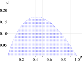
Figure 3: The graph of $g_{K(1,2)}(p)$.

Here, we choose $K^{\prime}$ to have $|{\rm VW}(K^{\prime})|=1$, $|{\rm VB}(K^{\prime})|=2$ and all edges are gray. That is, $K^{\prime}=K(1,2)$ and it is easy to see that $K_{3,3}\not\mapsto_{c}K^{\prime}$ . We can use Lemma 10 to compute that $g_{K^{\prime}}(p)=\frac{p(1-p)}{1+p}$. The maximum of this function on $[0,1]$ occurs at $(p^{*},d^{*})=\left(\sqrt{2}-1,3-2\sqrt{2}\right)$.

5.3.2 Lower bound

Fix $p^{*}=\sqrt{2}-1$. Let $K$ be any CRG for which $K_{3,3}\not\mapsto_{c}K$. For simplicity of notation, define $K_{\rm B}$ to be the CRG induced by ${\rm VB}(K)$. First we will give a lower bound on $p^{*}|{\rm EW}(K)|+(1-p^{*})|{\rm EB}(K)|$.

• In the CRG induced by ${\rm VW}(K)$, all edges must be white, otherwise $K_{3,3}\mapsto_{c}K$. These edges contribute a weight of $p^{*}\binom{|{\rm VW}(K)|}{2}$.

• In the bipartite CRG induced by $\left({\rm VW}(K),{\rm VB}(K)\right)$, if there is a triangle $\{b_{1},b_{2},b_{3}\}$ in ${\rm VB}(K)$ that has all edges white or gray then, for every $w\in{\rm VW}(K)$, $\{b_{i},w\}$ is white for at least one $i\in\{1,2,3\}$. Otherwise, $K_{3,3}\mapsto_{c}K$.
  Since there must be a white edge between every white/gray triangle in ${\rm VB}(K)$ and every vertex in ${\rm VW}(K)$, let $C\subseteq{\rm VB}(K)$ be a minimum-sized vertex set that contains a vertex from every triangle with no black edges in $K_{\rm B}$. These edges contribute a weight of at least $p^{*}|{\rm VW}(K)||C|$.

• Let $K_{{\rm B}\setminus{\rm C}}$ denote the CRG induced by ${\rm VB}(K)-C$. In $K_{\rm B}$, there can be no triangle with all edges gray, otherwise $K_{3,3}\mapsto_{c}K$. By the definition of $C$, in $K_{{\rm B}\setminus{\rm C}}$ there can be no triangle with all edges white or gray. These edges contribute a weight of at least

  $$\min\{p^{*},1-p^{*}\}\left(\binom{|{\rm VB}(K)|}{2}-t(|{\rm VB}(K)|,2)\right)$$

  $$+(1-2\min\{p^{*},1-p^{*}\})\left(\binom{|{\rm VB}(K)-C|}{2}-t(|{\rm VB}(K)-C|,2)\right).$$

Since $p^{*}<0.5$, $p^{*}|{\rm EW}(K)|+(1-p^{*})|{\rm EB}(K)|$ is at least

$$p^{*}\binom{|{\rm VW}(K)|}{2}+p^{*}|{\rm VW}(K)||C|+p^{*}\left(\frac{|{\rm VB}(K)|^{2}-2|{\rm VB}(K)|}{4}\right)$$

$$+(1-2p^{*})\left(\frac{|{\rm VB}(K)-C|^{2}-2|{\rm VB}(K)-C|}{4}\right).$$

A lower bound on $f_{K}(p^{*})$ gives

$$f_{K}(p^{*})k^{2} = p^{*}\left(|{\rm VW}(K)|+2|{\rm EW}(K)|\right)+(1-p^{*})\left(|{\rm VB}(K)|+2|{\rm EB}(K)|\right)$$ (3)

$$\geq p^{*}|{\rm VW}(K)|+(1-p^{*})|{\rm VB}(K)|+2p^{*}\binom{|{\rm VW}(K)|}{2}$$

$$+2p^{*}|{\rm VW}(K)||C|+2p^{*}\left(\frac{|{\rm VB}(K)|^{2}-2|{\rm VB}(K)|}{4}\right)$$

$$+2(1-2p^{*})\left(\frac{|{\rm VB}(K)-C|^{2}-2|{\rm VB}(K)-C|}{4}\right)$$

$$\geq (1-2p^{*})|C|+p^{*}|{\rm VW}(K)|^{2}+2p^{*}|{\rm VW}(K)||C|$$

$$+\frac{1-p^{*}}{2}|{\rm VB}(K)|^{2}-(1-2p^{*})|{\rm VB}(K)||C|+\frac{1-2p^{*}}{2}|C|^{2}$$

$$\geq p^{*}|{\rm VW}(K)|^{2}+\frac{1-p^{*}}{2}|{\rm VB}(K)|^{2}$$

$$+\frac{1-2p^{*}}{2}|C|\left(|C|-2|{\rm VB}(K)|+\frac{4p^{*}}{1-2p^{*}}|{\rm VW}(K)|\right).$$

All that remains is to verify that the expressions in (3) is at most $\frac{p^{*}(1-p^{*})}{1+p^{*}}k^{2}$. We need to divide this into two cases. First, assume $|{\rm VB}(K)|\leq\frac{2p^{*}}{1-2p^{*}}|{\rm VW}(K)|$. In this case, the value of $|C|$ that minimizes (3) is $|C|=0$,

$$f_{K}(p^{*})k^{2} \geq p^{*}|{\rm VW}(K)|^{2}+\frac{1-p^{*}}{2}|{\rm VB}(K)|^{2}$$

$$\geq \left(p^{*}\left(\frac{1-p^{*}}{1+p^{*}}\right)^{2}+\frac{1-p^{*}}{2}\left(\frac{2p^{*}}{1+p^{*}}\right)^{2}\right)k^{2}$$

$$= \frac{p^{*}(1-p^{*})}{1+p^{*}}k^{2}=(3-2\sqrt{2})k^{2},$$

because the minimum occurs at $|{\rm VB}(K)|=\frac{2p^{*}}{1+p^{*}}k$. Second, assume $|{\rm VB}(K)|\geq\linebreak[4]\frac{2p^{*}}{1-2p^{*}}|{\rm VW}(K)|$, i.e, $|{\rm VB}(K)|\geq 2p^{*}k$. In this case, the value of $|C|$ that minimizes (3) is $|C|=|{\rm VB}(K)|-\frac{2p^{*}}{1-2p^{*}}|{\rm VW}(K)|$:

$$f_{K}(p^{*})k^{2} \geq p^{*}|{\rm VW}(K)|^{2}+\frac{1-p^{*}}{2}|{\rm VB}(K)|^{2}-\frac{1-2p^{*}}{2}\left[|{\rm VB}(K)|-\frac{2p^{*}}{1-2p^{*}}|{\rm VW}(K)|\right]^{2}$$

$$= \left(p^{*}-\frac{2(p^{*})^{2}}{1-2p^{*}}\right)|{\rm VW}(K)|^{2}+\frac{p^{*}}{2}|{\rm VB}(K)|^{2}+2p^{*}|{\rm VW}(K)||{\rm VB}(K)|$$

$$= p^{*}k^{2}-\frac{2(p^{*})^{2}}{1-2p^{*}}|{\rm VW}(K)|^{2}-\frac{p^{*}}{2}|{\rm VB}(K)|^{2}.$$

This expression is minimized at the endpoints of the domain of $|{\rm VB}(K)|$. For $|{\rm VB}(K)|=k$, we have $\frac{p^{*}}{2}\approx 0.207>\frac{p^{*}(1-p^{*})}{1+p^{*}}=3-2\sqrt{2}\approx 0.172$. For the other endpoint, $|{\rm VB}(K)|=2p^{*}k$, we have

$$f_{K}(p^{*})k^{2}\geq p^{*}k^{2}-\frac{2(p^{*})^{2}}{1-2p^{*}}(1-2p^{*})^{2}k^{2}-\frac{p^{*}}{2}(2p^{*})^{2}k^{2}=\left[p^{*}-2(p^{*})^{2}+2(p^{*})^{3}\right]k^{2}.$$

This gives $f_{K}(p)\geq 15\sqrt{2}-21\approx 0.213>\frac{p^{*}(1-p^{*})}{1+p^{*}}=3-2\sqrt{2}\approx 0.172$.

To summarize, $f(p^{*})\geq\frac{p^{*}(1-p^{*})}{1+p^{*}}=3-2\sqrt{2}$. Therefore, $d^{*}({\rm Forb}(K_{3,3}))=3-2\sqrt{2}$ and $p^{*}({\rm Forb}(K_{3,3}))=\sqrt{2}-1$.

5.4 Edit distance of $H_{9}$

5.4.1 Upper bound

The Young tableau in Figure 5 diagrams the values of $(a,c)$ for which $H_{9}\not\mapsto_{c}K(a,c)$. To see this, we can exhibit the following partitions of $V(G)$:

• 3 cliques: $\left\{\{0,1,2\},\{3,4,5\},\{6,7,8\}\right\}$

• 1 coclique, 2 cliques: $\left\{\{2,7\},\{8,0,1\},\{3,4,5,6\}\right\}$

• 2 cocliques, 1 clique: $\left\{\{1,4,7\},\{2,5,8\},\{0,3,6\}\right\}$

• 4 cocliques: $\left\{\{1,4,7\},\{0,5\},\{3,8\},\{2,6\}\right\}$.

Moreover, it is easy to see that the largest clique of $H_{9}$ is 4 and the largest coclique is 3. So, $H_{9}\not\mapsto_{c}K(0,2),K(1,1)$. Since there are only two cocliques of size 3, $H_{9}\not\mapsto_{c}K(3,0)$.

Figure 5 gives the graphs of $g_{K(0,2)}(p)$, $g_{K(3,0)}(p)$ as well as $g_{K^{\prime\prime}}(p)$ for the $K^{\prime\prime}$ defined in the theorem. The region they define is shaded.

Figure 4: The Young tableau of $(a,c)$ for which $H_{9}\not\mapsto_{c}K(a,c)$.

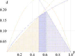
Figure 5: The graphs of the $g_{K}(p)$ relevant to $H_{9}$.

Recall that $K^{\prime\prime}$ satisfies $|{\rm VW}(K^{\prime\prime})|=4$, $|{\rm VB}(K^{\prime\prime})|=0$, one black edge and 5 gray edges. See Figure 6.

Figure 6: The colored regularity graph $K^{\prime\prime}$.

The graph $H_{9}$ has only two cocliques of order three: $\{1,4,7\}$ and $\{2,5,8\}$. The vertices that remain, $\{0,3,6\}$, form a clique. So, any partition of the vertices of $H_{9}$ into cocliques that uses both of these $3$-cocliques, requires 5 pieces to the partition. As a result, if there were a colored-homomorphism from $H_{9}$ into $K^{\prime\prime}$, it would partition the vertices into one coclique of order 3 and three cocliques of order 2.

Assuming such a colored-homomorphism exists, we assume, without loss of generality, that one of the cocliques is $\{1,4,7\}$. The vertex $0$ is only nonadjacent to $5$. The vertex $3$ is only nonadjacent to $8$. The vertex $6$ is only nonadjacent to $2$. Therefore, the only partition that can witness the colored-homomorphism is $\left\{\{1,4,7\},\{0,5\},\{2,6\},\{3,8\}\right\}$. Between every pair of these cocliques is a nonedge. So, no pair of them could be mapped to endpoints of the black edge of $K^{\prime\prime}$. Therefore, $H_{9}\not\mapsto_{c}K^{\prime\prime}$.

We can use Lemma 10 to conclude that $g_{K^{\prime}}(p)=\frac{1-p}{2}$ and $g_{K^{\prime\prime}}(p)=\frac{p}{2(1+p)}$. The intersection is at the point $(p,d)=\left(\frac{\sqrt{5}-1}{2},\frac{3-\sqrt{5}}{4}\right)$.

Thus, the upper bound obtained by $d^{*}\leq\max\limits_{p\in[0,1]}\min\limits_{(a,c):K(a,c)\in{\cal K}({\cal H})}g_{K(a,c)}(p)$ would be $1/5=0.2$, achieved by the intersection of $g_{K(0,2)}(p)=\frac{1-p}{2}$ and $g_{K(3,0)}(p)=\frac{p}{3}$. But, as we can see by Figure 5, the value $d=\frac{3-\sqrt{5}}{4}\approx 0.191$ provides a better upper bound.

5.5 New proof of the edit distance of $\overline{P_{3}+K_{1}}$

Alon and Stav [2] computed $(p^{*},d^{*})$ for hereditary properties defined by graphs on at most $4$ vertices. This paper has also done so, as a corollary of our results, with the exception of ${\rm Forb}\left(\overline{P_{3}+K_{1}}\right)$. We include a computation of the value of $(p^{*},d^{*})$ as an application of our technique and to demonstrate the versatility of Lemma 18.

5.5.1 Upper bound

Here, we choose $K^{\prime}=K(0,1)$ and $K^{\prime\prime}=K(2,0)$. Recall that $\overline{P_{3}+K_{1}}$ is a triangle with a pendant edge. It is easy to see that both $\overline{P_{3}+K_{1}}\not\mapsto_{c}K^{\prime}$ and $\overline{P_{3}+K_{1}}\not\mapsto_{c}K^{\prime\prime}$. We can use Lemma 10 to conclude that $g_{K^{\prime}}(p)=1-p$ and $g_{K^{\prime\prime}}(p)=\frac{p}{2}$. The intersection is at the point $(p^{*},d^{*})=\left(\frac{2}{3},\frac{1}{3}\right)$. Clearly, this $p^{*}$ is unique because $g(p)<1/3$ for all $p\neq 2/3$.

5.5.2 Lower bound

Fix $p^{*}=\frac{2}{3}$. Let $K$ be any CRG for which $\overline{P_{3}+K_{1}}\not\mapsto_{c}K$. For simplicity of notation, define $K_{\rm W}$ to be the CRG induced by ${\rm VW}(K)$. We will give a lower bound on $p^{*}|{\rm EW}(K)|+(1-p^{*})|{\rm EB}(K)|$.

• In the bipartite CRG induced by $({\rm VW}(K),{\rm VB}(K))$, no edges can be gray, otherwise $\overline{P_{3}+K_{1}}\mapsto_{c}K$. This contributes $\min\{p^{*},1-p^{*}\}|{\rm VW}(K)||{\rm VB}(K)|$.

• In the CRG induced by ${\rm VB}(K)$, no edges can be gray, otherwise $\overline{P_{3}+K_{1}}\linebreak\mapsto_{c}K$. This contributes $\min\{p^{*},1-p^{*}\}\binom{|{\rm VB}(K)|}{2}$.

• In $K_{\rm W}$, consider any subset of $3$ vertices. If there is neither a white edge nor a pair of black edges, then it is possible to map the vertices of $\overline{P_{3}+K_{1}}$ into those three vertices so that each vertex of the triangle is mapped to a different vertex and the pendant vertex is in the vertex incident to the two gray edges. This contributes $p^{*}{\rm EW}(K_{\rm W})+(1-p^{*}){\rm EB}(K_{\rm W})$.

To summarize, using $p^{*}=2/3$ and Lemma 18, we have

$$p^{*}|{\rm EW}(K)|+(1-p^{*})|{\rm EB}(K)|$$

$$\geq \frac{1}{3}\left(|{\rm VW}(K)||{\rm VB}(K)|+\binom{|{\rm VB}(K)|}{2}\right)+\frac{1}{3}\left(2|{\rm EW}(K_{\rm W})|+|{\rm EB}(K_{\rm W})|\right)$$

$$\geq \frac{1}{3}\left(|{\rm VW}(K)||{\rm VB}(K)|+\binom{|{\rm VB}(K)|}{2}\right)+\frac{1}{3}\left\lceil\frac{|{\rm VW}(K)|}{2}(|{\rm VW}(K)|-2)\right\rceil$$

$$= \frac{1}{3}\left(|{\rm VW}(K)||{\rm VB}(K)|+\binom{|{\rm VB}(K)|}{2}+\frac{|{\rm VW}(K)|^{2}-2|{\rm VW}(K)|}{2}\right).$$

Now we give a lower bound on $f_{K}(p^{*})$:

$$f_{K}(p^{*})k^{2} = p^{*}\left(|{\rm VW}(K)|+2|{\rm EW}(K)|\right)+(1-p^{*})\left(|{\rm VB}(K)|+2|{\rm EB}(K)|\right)$$

$$\geq \frac{2}{3}|{\rm VW}(K)|+\frac{1}{3}|{\rm VB}(K)|+\frac{2}{3}\left(|{\rm VW}(K)||{\rm VB}(K)|\right.$$

$$+\left.\frac{|{\rm VB}(K)|^{2}-|{\rm VB}(K)|}{2}+\frac{|{\rm VW}(K)|^{2}-2|{\rm VW}(K)|}{2}\right)$$

$$= \frac{1}{3}\left(|{\rm VW}(K)|^{2}+2|{\rm VW}(K)||{\rm VB}(K)|+|{\rm VB}(K)|^{2}\right)=\frac{1}{3}k^{2}.$$

So, comparing with the upper bound, $d^{*}({\rm Forb}(\overline{P_{3}+K_{1}}))=1/3$ and since $g(p)\leq\min\{g_{K^{\prime}}(p),$ $g_{K^{\prime\prime}}(p)\}<1/3$ for all $p\neq 2/3$, it is also the case that $p^{*}({\rm Forb}(\overline{P_{3}+K_{1}}))=2/3$. $\Box$

6 Conclusions

6.1 Observations on functions $f$ and $g$

The function $f_{K}(p)$ is invariant under equipartitions of $V(K)$. To see this, let $\tilde{K}$ be formed by partitioning each vertex of $K$ into $c$ pieces with the colors of vertices and edges be the natural coloring inherited from $K$. As a result, $|{\rm VW}(\tilde{K})|=c|{\rm VW}(K)|$, $|{\rm VB}(\tilde{K})|=c|{\rm VB}(K)|$, $|{\rm EW}(\tilde{K})|=c^{2}|{\rm EW}(K)|+\binom{c}{2}|{\rm VW}(K)|$ and $|{\rm EB}(\tilde{K})|=c^{2}|{\rm EB}(K)|+\binom{c}{2}|{\rm VB}(K)|$. Thus,

$$f_{\tilde{K}}(p)=\frac{1}{c^{2}k^{2}}\left[p(|{\rm VB}(\tilde{K})|+2|{\rm EW}(\tilde{K})|)+(1-p)(|{\rm VW}(\tilde{K})|+2|{\rm EB}(\tilde{K})|)\right]\\ =f_{K}(p).$$

The same is true for $g_{K}(p)$ and $g_{\tilde{K}}(p)$. Any feasible solution, ${\bf u}$ of the quadratic program that defines $g_{K}(p)$ can be made into a feasible solution, $\tilde{{\bf u}}$ of the quadratic program that defines $g_{\tilde{K}}(p)$ by arbitrarily distributing the weight of one vertex in $K$ to the vertices in $\tilde{K}$ to which it corresponds. It can be seen that, if ${\bf M}_{K}(p)$ is the matrix corresponding to $K$ and ${\bf M}_{\tilde{K}}(p)$ is the matrix corresponding to $\tilde{K}$, then ${\bf u}^{T}{\bf M}_{K}(p){\bf u}=\tilde{{\bf u}}^{T}{\bf M}_{\tilde{K}}(p)\tilde{{\bf u}}$.

The function $g$ is more flexible, however. It is not only invariant under equipartitions but it is invariant under arbitrary partitions. To see this, construct an equivalence relation on the vertices of a CRG, $K$, in which vertices $u$ and $v$ are equivalent if $u$, $v$ and $\{u,v\}$ are all the same color and, for all $w\in V(K)-\{u,v\}$, $\{u,w\}$ and $\{v,w\}$ are the same color as each other.

If $K$ is a CRG and $K_{0}$ is the CRG induced by the equivalence relation on $K$, then $g_{K}(p)=g_{K_{0}}(p)$. Therefore, in the computation of $g(p)$, one may ignore CRGs which have nontrivial equivalence classes.

6.2 Open questions

• Investigating Proposition 17, is there a more convenient expression for the upper bound based only on the Young diagram (see Figures 3 and 5) of the set of CRGs $\{K(a,c):H\not\mapsto_{c}K(a,c),\forall H\in{\cal F}({\cal H})\}$?

• To compute the edit distance is hard, we do not have sharp result even for ${\rm Forb}(K_{m,n})$, where $K_{m,n}$ is an arbitrary complete bipartite graph.

• The precise value for $d^{*}(H_{9})$, where $H_{9}$ is defined in Theorem 14, is unknown, but we conjecture that the upper bound is correct and we further conjecture that $p^{*}({\rm Forb}(H_{9}))=(\sqrt{5}-1)/2$.

• Every hereditary property ${\cal H}$ can be expressed as $\bigcap_{H\in{\cal F}({\cal H})}{\rm Forb}(H)$ for some family of graphs ${\cal F}({\cal H})$. In computing edit distance, it may be that some members of $H\in{\cal F}({\cal H})$ are unnecessary, even if they are necessary to define the family. I.e, for hereditary property ${\cal H}$, what are the maximal properties ${\cal H}^{\prime}\supseteq{\cal H}$ such that $d^{*}({\cal H}^{\prime})=d^{*}({\cal H})$?

  For example, the strong perfect graph theorem [11] states that perfect graphs are characterized by ${\cal P}=\bigcap_{k\geq 2}\left({\rm Forb}(C_{2k+1})\cap{\rm Forb}(\overline{C_{2k+1}})\right)$. But, it is not difficult to use Theorem 16 to show that $d^{*}({\cal P})=d^{*}({\rm Forb}(C_{5}))=1/4$, as observed by Alon and Stav [1].

• Our proofs of the lower bounds for $d^{*}({\rm Forb}(H))$ for $H=K_{a}+E_{b}$ or $H=K_{3,3}$ are cumbersome and cannot assume that the total number of vertices in each of the forbidden CRGs is bounded by any function of $H$. Is there a better way to compute the lower bound? Is there a function of $H$ so that we need only to consider $g_{K}(p)$ for $K$ whose order is bounded by said function?

• Finally, the edit distance is unknown for most hereditary properties. So-called unit disk graphs (UDGs), see [12], define a hereditary property but the family ${\cal F}$ is not known. It is easy to see that $K_{1,7}$ cannot occur as an induced subgraph in a UDG. (For some definitions of the unit disk graph, $K_{1,6}$ is forbidden also.) We believe that a small family of such forbidden induced subgraphs will be enough to determine the edit distance from the family of UDGs.

  For any graph $H$, both $p^{*}({\rm Forb}(H))$ and $d^{*}({\rm Forb}(H))$ can be considered invariants of graph $H$. Being able to compute these invariants even for some given fixed graph seems to be quite difficult in general.

6.3 Thanks

We thank Maria Axenovich for valuable conversations. We also thank Noga Alon for reading a draft of the paper and making several useful comments. These include the observation that the existence of the limit that defines $d^{*}({\cal H})$ results from a simple monotonicity argument. We appreciate the careful reading of an anonymous referee, which lead to improvements in the manuscript.

References

- [1] N. Alon and U. Stav, What is the furthest graph from a hereditary property?, to appear in Random Structures Algorithms.
- [2] N. Alon and U. Stav, The maximum edit distance from hereditary graph properties, to appear in J. Combin. Theory Ser. B.
- [3] M. Axenovich and R. Martin, Avoiding patterns in matrices via a small number of changes, SIAM J. Discrete Math., 20 (2006), no. 1, 49–54.
- [4] M. Axenovich, A. Kézdy and R. Martin, On the editing distance in graphs, to appear in J. Graph Theory.
- [5] B. Bollobás, Hereditary properties of graphs: asymptotic enumeration, global structure, and colouring. Proceedings of the international Congress of Mathematicians, Vol. III (Berlin 1998). Doc. Math. 1998, Extra Vol. III, 333–342 (electronic).
- [6] B. Bollobás, Modern graph theory, Graduate texts in mathematics, 184. Springer-Verlag, New York, 1998. xiv+394 pp.
- [7] B. Bollobás, Random graphs. Second edition. Cambridge Studies in Advanced Mathematics, 73. Cambridge University Press, Cambridge, 2001. xviii+498 pp.
- [8] B. Bollobás and A. Thomason, Projections of bodies and hereditary properties of hypergraphs. Bull. London Math. Soc. 27 (1995), no. 5, 417–424.
- [9] B. Bollobás and A. Thomason, Hereditary and monotone properties of graphs. The mathematics of Paul Erdős, II 70–78, Algorithms Combin., 14, Springer, Berlin, 1997.
- [10] B. Bollobás and A. Thomason, The structure of hereditary properties and colourings of random graphs. Combinatorica 20 (2000), no. 2, 173–202.
- [11] M. Chudnovsky, N. Robertson, P. Seymour and R. Thomas, The strong perfect graph theorem. Ann. of Math. (2) 164 (2006), no. 1, 51–229.
- [12] B.N. Clark, C.J. Colbourn and D.S. Johnson, Unit disk graphs. Discrete Math. 86 (1990), no. 1 3, 165 -177.
- [13] P. Erdős and A. Rényi, On random graphs I. Publ. Math. Debrecen 6 (1959), 290–297.
- [14] P. Erdős and M. Simonovits, A limit theorem in graph theory, Studia Sci. Math. Hungar 1 (1966), 51–57.
- [15] P. Erdős and A. Stone, On the structure of linear graphs, Bull. Amer. Math. Soc. 52 (1946), 1087–1091.
- [16] S. Janson, T. Łuczak and A Ruciński, Random Graphs. Wiley-Interscience Series in Discrete Mathematics and Optimization. Wiley-Interscience, New York, 2000.
- [17] J. Komlós, A. Shokoufandeh, M. Simonovits and E. Szemerédi, The regularity lemma and its applications in graph theory. Theoretical aspects of computer science (Tehran, 2000), 84–112, Lecture Notes in Comput. Sci., 2292, Springer, Berlin, 2002.
- [18] J. Komlós and M. Simonovits, Szemerédi’s regularity lemma and its applications in graph theory. Combinatorics, Paul Erdős is eighty, Vol. 2 (Keszthely, 1993), 295–352, Bolyai Soc. Math. Stud. 2, János Bolyai Math. Soc., Budapest, 1996.
- [19] H.J. Prömel and A. Steger, Excluding induced subgraphs: quadrilaterals. Random Structures Algorithms 2 (1991), no. 1, 55–71.
- [20] H.J. Prömel and A. Steger, Excluding induced subgraphs. II. Extremal graphs. Discrete Appl. Math. 44 (1993), no. 1-3, 283–294.
- [21] H.J. Prömel and A. Steger, Excluding induced subgraphs. III. A general asymptotic. Random Structures Algorithms 3 (1992), no. 1, 19–31.
- [22] W. Rudin, Principles of mathematical analysis. Third edition. International Series in Pure and Applied Mathematics. McGraw-Hill Book Co., New York-Auckland-Düsseldorf, 1976. x+342 pp.
- [23] E. Szemerédi, On sets of integers containing no elements in arithmetic progression, Acta Arithmetica 27 (1975), 199–245.
- [24] E. Szemerédi, Regular partitions of graphs. In Problèmes Combinatoires et Théorie des Graphes, 399–401, Colloq. Internat. CNRS, Univ. Orsay, Paris, 1978.
- [25] P. Turán, Eine Extremalaufgabe aus der Graphentheorie. (Hungarian) Mat. Fiz. Lapok 48, (1941), 436–452.