Superconductivity in FeSe thin films driven by the interplay between nematic fluctuations and spin-orbit coupling

Abstract

The origin of the high-temperature superconducting state observed in FeSe thin films, whose phase diagram displays no sign of magnetic order, remains a hotly debated topic. Here we investigate whether fluctuations arising due to the proximity to a nematic phase, which is observed in the phase diagram of this material, can promote superconductivity. We find that nematic fluctuations alone promote a highly degenerate pairing state, in which both $s$-wave and $d$-wave symmetries are equally favored, and $T_{c}$ is consequently suppressed. However, the presence of a sizable spin-orbit coupling or inversion symmetry-breaking at the film interface lifts this harmful degeneracy and selects the $s$-wave state, in agreement with recent experimental proposals. The resulting gap function displays a weak anisotropy, which agrees with experiments in monolayer FeSe and intercalated Li_1-x(OH)_xFeSe.

In most iron-based superconductors (FeSC), superconductivity is found in close proximity to a magnetically ordered state, suggesting that magnetic fluctuations play an important role in binding the Cooper pairs Mazin08 ; Hirschfeld11 ; Chubukov11 ; Chubukov_review . Indeed, the fact that the Fermi surface of these materials is composed of small hole pockets and electron pockets separated by the magnetic ordering vector led to the proposal of a sign-changing $s^{+-}$ wave state, in which the gap function has different signs in the hole and in the electron pockets. However, the recent observation of superconductivity over $70$ K in monolayer FeSe brought new challenges to the field Xue12 ; Feng12 ; Zhou13 ; Feng13 ; Xue14 ; Jia14 ; Wang14 ; Ding15 ; FengNC14 ; Chen16 . In contrast to the standard FeSC, no long-range magnetic order is observed in thin films or even bulk FeSe Khasanov09 , and the Fermi surface of monolayer FeSe consists of electron pockets only Zhou13 ; Feng12 ; Shen14 ; Ding15 . Since $T_{c}$ in monolayer FeSe is the highest among all FeSC, the elucidation of its origin is a fundamental step in the search for higher $T_{c}$ in these systems.

One of the proposed scenarios to explain the dramatic ten-fold increase of $T_{c}$ in monolayer FeSe with respect to the $8$ K value in bulk FeSe HSU08 was the strong coupling to an optical phonon mode of the SrTiO₃ (STO) substrate Shen14 ; Lee12 ; Zhao16 , which is manifested by replica bands observed in ARPES Shen14 . Although such a coupling can certainly enhance $T_{c}$ Rademaker16 ; DHLee_STO ; Millis16 ; Johnston16 ; Dolgov16 , recent experiments indicate that the STO substrate may not be essential to achieve the high-$T_{c}$ state. In particular, $T_{c}$ up to $40$ K was observed in electrostatically-gated films of FeSe with different thickness grown both on STO and MgO substrates Tsukazaki16 . Similar values of $T_{c}$ were reported in FeSe coated with potassium Takahashi15 ; ShenSC15 and in the bulk sample Li_1-x(OH)_xFeSe FengPRB15 ; Zhou16 , which consists of intercalated FeSe layers. In common to all these systems is the fact that their Fermi surface consists of electron pockets only, suggesting that doping by negative charge carriers plays a fundamental role in stabilizing the high-$T_{c}$ state.

Importantly, recent experiments in K-coated bulk FeSe ShenSC15 revealed that, besides shifting the chemical potential, electron-doping also suppresses the nematic order observed in undoped bulk FeSe at $T_{\mathrm{nem}}\approx 90$ K Coldea15 . In the nematic state, whose origin remains hotly debated RMF15 ; RMF16 ; Si15 ; DHLee_FeSe15 ; Glasbrenner15 , the $x$ and $y$ in-plane directions become inequivalent and orbital order emerges. Remarkably, the highest $T_{c}$ in the phase diagram of K-coated FeSe is observed near the region where $T_{\mathrm{nem}}$ nearly vanishes. Similarly, in the case of FeSe thin films grown on STO, nematic order is observed over a wide range of film thickness ShenNem15 ; Feng16 , but not in the monolayer case Hoffman16 . These observations, combined with the absence of magnetic order in these systems, begs the question of whether nematic fluctuations can provide a sensible mechanism to explain the superconductivity of thin films of FeSe ShenSC15 ; Yamase13 ; DHLee_STO ; Vishwanath15 .

In this paper, we show that nematic fluctuations alone favor degenerate $s$-wave ($A_{1g}$) and $d$-wave ($B_{2g}$) superconducting states in FeSe thin films. This degeneracy stems from the fact that while the two electron pockets are separated by the momentum $\boldsymbol{Q}_{M}=\left(\pi,\pi\right)$, nematic fluctuations are peaked at $\boldsymbol{Q}_{\mathrm{nem}}=0$. More importantly, the SC ground state manifold has an enlarged $U(1)\times U(1)$ degeneracy, which is very detrimental to SC, since fluctuations of one SC channel strongly suppress long-range order in the other SC channel. Remarkably, this degeneracy is removed by the sizable spin-orbit coupling (SOC) observed in these compounds Zhigadlo16 , which lift the pairing frustration and selects $s$-wave over $d$-wave, stabilizing a SC state at higher temperatures. In thin films, the inversion symmetry-breaking (ISB) at the interface also contributes significantly to this degeneracy lifting. Interestingly, recent experiments propose that an $s$-wave state is realized in FeSe thin films FengNP15 . We also find that, when the SOC and/or ISB energy scales are larger than the energy scale associated with the mismatch between the two electron pockets, a nearly isotropic gap appears at the electron pockets, whose angular dependence agrees with ARPES and STM measurements in FeSe thin films ShenSC15 ; FengPRL14 and intercalated Li_1-x(OH)_xFeSe Wen16 .

Microscopic model   We start with the full five-orbital tight-binding model in the 1-Fe Brillouin zone and project it on the subspace of the $d_{xz}$, $d_{yz}$, and $d_{xy}$ orbitals, which give the largest contribution to the Fermi surface. In particular, while the $X$ electron pocket centered at $\boldsymbol{Q}_{X}=(\pi,0)$ has $d_{yz}/d_{xy}$ orbital content, the $Y$ electron pocket centered at $\boldsymbol{Q}_{Y}=(0,\pi)$ has $d_{xz}/d_{xy}$ content (see Fig. 1a). Following Ref. Oskar13 , we expand the projected tight-binding matrix in powers of the momentum measured relative to $\boldsymbol{Q}_{X}$ and $\boldsymbol{Q}_{Y}$. Defining two spinors corresponding to each electron pocket:

$$\Psi_{X}(\boldsymbol{k}) \approx \left(d_{yz}(\boldsymbol{k}+\boldsymbol{Q}_{X})\ ,\ d_{xy}(\boldsymbol{k}+\boldsymbol{Q}_{X})\right)^{T}$$

$$\Psi_{Y}(\boldsymbol{k}) \approx \left(d_{xz}(\boldsymbol{k}+\boldsymbol{Q}_{Y})\ ,\ d_{xy}(\boldsymbol{k}+\boldsymbol{Q}_{Y})\right)^{T}$$ (1)

the non-interacting Hamiltonian is written as $\mathcal{H}_{0}=\sum\limits_{\boldsymbol{k},i=X,Y}\Psi_{i}^{\dagger}(\boldsymbol{k})\hat{H}_{i}(\boldsymbol{k})\Psi_{i}(\boldsymbol{k})$ where $\hat{H}_{i}$ are $2\times 2$ matrices in spinor space (see the supplementary material SM). The $B_{2g}$ nematic order parameter is described by the bosonic field $\phi_{q}$, with $q=\left(\Omega_{n},\boldsymbol{q}\right)$, whereas the nematic fluctuations are given by the nematic susceptibility $\chi_{\mathrm{nem}}(\boldsymbol{q},\Omega_{n})$. For our analysis, it is not necessary to specify the origin of the nematic order parameter, but rather how it couples to the electronic states. As discussed in Ref. Vafek14 , there are two possible nematic couplings: $\lambda_{1}$, which couples $\phi_{q}$ to the onsite energy difference between the $d_{xz}$ and $d_{yz}$ orbitals, and $\lambda_{2}$, which couples $\phi_{q}$ to the hopping anisotropy between nearest-neighbor $d_{xy}$ orbitals (see Fig. 1b):

$$\mathcal{H}_{\mathrm{int}}=\sum_{\boldsymbol{q},i=X,Y}\phi_{-\mathbf{q}}\Psi_{i}^{\dagger}(\boldsymbol{k})\hat{\lambda}_{i}^{\mathrm{nem}}\Psi_{i}(\boldsymbol{k}+\boldsymbol{q})$$ (2)

with $\hat{\lambda}_{i}^{\mathrm{nem}}=\pm\mathrm{diag}\left(\lambda_{1},\lambda_{2}\right)$, where the plus (minus) sign refers to $i=X$ ($i=Y)$. Here, we focus on the effect of short-ranged frequency independent nematic fluctuations and approximate $\chi_{\mathrm{nem}}(\boldsymbol{q},\Omega_{n})$ by its zero momentum and zero frequency value. The first approximation is justified due to the smallness of the electron pockets, whereas the second one is reasonable as long as the system is not too close to a nematic quantum critical point Schattner15 ; DHLee15 ; Vishwanath15 . Note that renormalization-group calculations on a related microscopic model support the idea that the disappearance of the central hole pockets suppresses nematic order RMF16 .

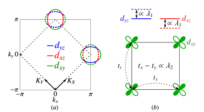
Figure 1: (a) Fermi surface (FS) of a thin film of FeSe, consisting only of electron pockets, in the unfolded (solid lines) and folded (dotted lines) Brillouin zones. The color around the FS indicates the orbital that contributes the largest spectral weight. (b) The two different nematic couplings: $\lambda_{1}$ couples to the on-site energy difference between the $d_{xz}$ and $d_{yz}$ orbitals, whereas $\lambda_{2}$ couples to the anisotropic hopping between nearest-neighbor $d_{xy}$ orbitals.

Superconducting instability   We decompose the pairing states in terms of the different irreducible representations of the space group of the FeSe plane, $P4/nmm$ (see Ref. Oskar13 and the SM), and focus on the two leading pairing channels, which belong to the singlet $s$-wave ($A_{1g}$) and $d$-wave ($B_{2g}$) symmetry representations note :

$$\Psi_{X}^{T}\begin{pmatrix}\Delta_{1}&0\\ 0&\Delta_{2}\end{pmatrix}\otimes i\sigma_{2}\Psi_{X}\pm\Psi_{Y}^{T}\begin{pmatrix}\Delta_{1}&0\\ 0&\Delta_{2}\end{pmatrix}\otimes i\sigma_{2}\Psi_{Y}$$ (3)

where the plus (minus) sign refers to $s$-wave ($d$-wave) pairing. The gaps $\Delta_{1}$ and $\Delta_{2}$ correspond to intra-orbital pairing within the $d_{xz}/d_{yz}$ orbitals and $d_{xy}$ orbitals, respectively.$\Delta_{1}$ and $\Delta_{2}$ are found via the gap equations:

$$\eta\hat{M}=\chi_{\mathrm{nem}}T\sum_{n,\boldsymbol{k}}\left(\hat{\lambda}_{i}^{\mathrm{nem}}\right)^{T}\hat{G}_{-k,i}^{T}\hat{M}\hat{G}_{k,i}\hat{\lambda}_{i}^{\mathrm{nem}}$$ (4)

where $\eta$ is the SC eigenvalue, $\hat{M}=\begin{pmatrix}\Delta_{1}&0\\ 0&\Delta_{2}\end{pmatrix}$, and $\hat{G}_{p,i}^{-1}=i\omega_{n}-\hat{H}_{i}\left(\mathbf{p}\right)$. The SC transition temperature is obtained when $\eta=1$. Hereafter, we set the value of $\left(\lambda_{1}^{2}+\lambda_{2}^{2}\right)\chi_{\mathrm{nem}}$ to yield $T_{c}=5$meV when $\lambda_{2}=0$.

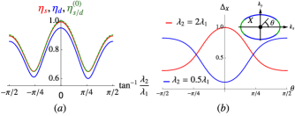
Figure 2: (a) The eigenvalue $\eta$ of the gap equation (4) as function of the ratio between the two nematic couplings $\lambda_{2}/\lambda_{1}$. Without SOC or ISB, the $s$-wave and $d$-wave solutions have the same eigenvalue (dashed green curve, $\eta_{s/d}^{(0)}$ ). The presence of SOC or ISB removes this degeneracy, making $s$-wave (red curve, $\eta_{s}$) the leading pairing instability and $d$-wave (blue curve, $\eta_{d}$) the subleading one. (b) Normalized SC gap along the $X$ electron pocket as function of the angle $\theta$ for different values of $\lambda_{2}/\lambda_{1}$.

Solution of the gap equations reveals that for all ratios of the nematic coupling constants $\lambda_{1}$ and $\lambda_{2}$, the superconducting instabilities in the $s$-wave and $d$-wave channels are always degenerate, as shown in Fig. 2a. Although the intra-orbital gaps $\Delta_{1}$ and $\Delta_{2}$ are isotropic, the gaps projected onto the Fermi pockets, $\Delta_{X}$ and $\Delta_{Y}$, acquire an angle-dependence due to the orbital content of the Fermi pockets. To illustrate this behavior, Fig. 2b shows $\Delta_{X}$ as function of the polar angle $\theta$. When $\lambda_{1}>\lambda_{2}$, nematic fluctuations couple mainly to the $d_{xz}/d_{yz}$ orbitals; as a result, $\Delta_{X}$ is proportional to the spectral weight of the $d_{xz}/d_{yz}$ orbital on the $X$ pockets, which is maximum around $\theta=\pm\pi/2$ (see Fig. 1a). Consequently, $\Delta_{X}$ reaches its maximum at $\theta=\pm\pi/2$ and its minimum at $\theta=0,\pi$. Conversely, for $\lambda_{1}<\lambda_{2}$, the gap is maximum at $\theta=0,\pi$, where the spectral weight of the $d_{xy}$ orbital on the $X$ pocket is maximum. Recent ARPES experiments in FeSe suggest that $\lambda_{1}$ and $\lambda_{2}$ are comparable Borisenko .

In terms of the averaged gaps $\Delta_{X}$ and $\Delta_{Y}$, the $s$-wave and $d$-wave solutions correspond to $\Delta_{s}=\frac{1}{2}(\Delta_{X}+\Delta_{Y})$ and $\Delta_{d}=\frac{1}{2}(\Delta_{X}-\Delta_{Y})$. Using this notation, the degeneracy between $s$ and $d$ can be understood as a consequence of the fact that nematic fluctuations, peaked at $\boldsymbol{Q}_{\mathrm{nem}}=0$, do not couple the gaps at the $X$ and $Y$ pockets, since they are displaced by the momentum $\mathbf{Q}_{M}=\mathbf{Q}_{X}+\mathbf{Q}_{Y}=(\pi,\pi)$. This suggests an enlarged $U(1)\times U(1)$ degeneracy of the SC ground state manifold, corresponding to two decoupled SC order parameters. To investigate the robustness of this enlarged degeneracy, we went beyond the linearized gap equations and computed the superconducting free energy to quartic order in the gaps (see SM), obtaining:

$$F_{SC}=a\left(|\Delta_{X}|^{2}+|\Delta_{Y}|^{2}\right)+\frac{u}{2}\left(|\Delta_{X}|^{4}+|\Delta_{Y}|^{4}\right)$$ (5)

This form confirms that $\Delta_{X}$ and $\Delta_{Y}$ remain decoupled to higher orders in $F_{SC}$. The consequences of this enlarged $U(1)\times U(1)$ degeneracy are severe: going beyond the mean-field approximation of Eq. (4), fluctuations of one SC channel suppress long-range order in the other channel, i.e. $T_{c,s}-T_{c,0}\propto-\left\langle\Delta_{d}^{2}\right\rangle$. Such a pairing frustration is therefore detrimental to SC DHLee_13 ; Fernandes13 ; Brydon14 ; YXWang16 , suggesting that nematic fluctuations alone do not provide an optimal SC pairing mechanism in this system. Interestingly, previous investigations of SC induced by nematic fluctuations in different models also found nearly-degenerate states Yamase13 ; Kivelson15 .

Spin-orbit coupling (SOC) and Inversion symmetry-breaking (ISB)   The analysis above neglected a key property of the crystal structure of the FeSe plane: Because of the puckering of the Se atoms above and below the Fe square lattice, the actual crystallographic unit cell contains 2 Fe atoms. As a result, in the 2-Fe Brillouin zone (the folded BZ), the momentum $\boldsymbol{Q}_{M}=\left(\pi,\pi\right)$ becomes $\mathbf{\tilde{Q}}=0$ (hereafter the tilde denotes a wave-vector in the folded BZ). Thus, the two electron pockets become centered at the same momentum $\tilde{\mathbf{Q}}=\left(\pi,\pi\right)$ and overlap, as shown by the dashed lines in Fig. 1a.

This property opens up the possibility of coupling the $\Delta_{X}$ and $\Delta_{Y}$ gaps and removing the enlarged $U(1)\times U(1)$ degeneracy. At the non-interacting level, this is accomplished by the atomic spin orbit coupling $\lambda_{\mathrm{SOC}}\boldsymbol{S}\cdot\boldsymbol{L}$, which couples the $d_{xz}$ ($d_{yz}$) orbital associated with the $Y$ ($X$) pocket to the $d_{xy}$ orbital associated with the $X$ ($Y$) pocket Vafek14 :

$$\mathcal{H}_{\mathrm{SOC}}=\frac{i}{2}\lambda_{\mathrm{SOC}}\sum_{\boldsymbol{k}}\Psi_{Y}^{{\dagger}}\left(\tau_{+}\otimes\sigma_{1}+\tau_{-}\otimes\sigma_{2}\right)\Psi_{X}+h.c.$$ (6)

where $\tau$ and $\sigma$ are Pauli matrices in spinor and spin spaces, respectively. While in the normal state the SOC splits the two overlapping elliptical electron pockets centered at $\tilde{\mathbf{Q}}=\left(\pi,\pi\right)$ into inner and outer pockets (see Fig. 3a and the ARPES data of Zhigadlo16 ), in the SC state it couples the gaps $\Delta_{X}$ and $\Delta_{Y}$. For $\lambda_{\mathrm{SOC}}$ small compared to $\epsilon_{m}$ – the energy scale associated with the mismatch between the $X$ and $Y$ electron pockets – this coupling is given perturbatively by the Feynman diagram of Fig. 3b, which gives the following contribution to the SC free energy of Eq. (5):

$$\delta F_{SC}=\gamma\left(\Delta_{X}\Delta_{Y}^{*}+h.c\right)$$ (7)

As shown in the SM, $\gamma\propto-\lambda^{2}$, implying that the SOC selects the $s$-wave state, with $\Delta_{X}$ and $\Delta_{Y}$ of the same sign, over the $d$-wave state, with $\Delta_{X}$ and $\Delta_{Y}$ of opposite signs. More importantly, it lifts the $U(1)\times U(1)$ degeneracy between the two pairing states, suppressing the negative interference of one pairing channel on the other. We confirmed this general conclusion by evaluating explicitly the gap equations in the $A_{1g}$ ($s$-wave) and $B_{2g}$ ($d$-wave) channels, finding that $\eta_{s}>\eta_{d}$ for all values of the nematic coupling constants, as shown in Fig. 2a. Note that the SOC induces triplet components to these pairing states (see SM).

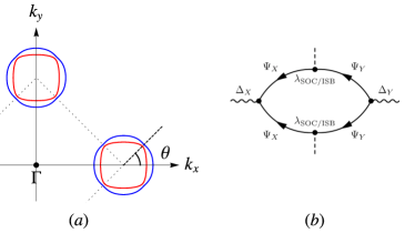
Figure 3: (a) The Fermi surface in the presence of SOC or ISB consists of split inner (red) and outer (blue) electron pockets. (b) Feynman diagram representing the coupling between the gaps in the two electron pockets promoted by SOC or ISB. This coupling lifts the degeneracy between $s$-wave and $d$-wave.

Having established that the $A_{1g}$ channel is the leading SC instability, we now discuss the angular dependence of the gaps $\Delta_{i/o}$ around the inner ($i$) and outer ($o$) electron pockets. When $\lambda_{\mathrm{SOC}}\ll\epsilon_{m}$, as it is apparent from Fig. 1a, the outer electron pocket consists mostly of $d_{xy}$ orbital spectral weight, whereas the inner pocket consists mostly of $d_{xz}/d_{yz}$ spectral weigh. The $d_{xz}$ and $d_{yz}$ gap functions have essentially the same angular dependence as in the case without SOC, shown previously in Fig. 2b. Consequently, the gap anisotropy depends strongly on the ratio $\lambda_{1}/\lambda_{2}$ between the two nematic couplings. For $\lambda_{1}\approx\lambda_{2}$, the gaps are nearly isotropic around the inner and outer pockets, whereas for $\lambda_{1}<\lambda_{2}$ or $\lambda_{1}>\lambda_{2}$, the gaps are anisotropic in both pockets.

The gap structure however changes dramatically in the case $\lambda_{\mathrm{SOC}}\gg\epsilon_{m}$ (with both still much smaller than the Fermi energy). In this case, the two reconstructed electron pockets are fully hybridized, implying that their orbital weights are similar. As a result, the SC gaps on the inner and outer pockets are weakly anisotropic for all values of the ratio $\lambda_{1}/\lambda_{2}$, whose main effect is to displace the position of the gap maxima. While for $\lambda_{1}<\lambda_{2}$ the gap minima are located at the intersection points between the two un-hybridized electron pockets, $\theta=\pm\pi/4$, for $\lambda_{1}>\lambda_{2}$ the gap minima are found at the intersection points (see Fig. 4). Interestingly, recent ARPES experiments in monolayer FeSe observe gap maxima at $\theta=\pm\pi/4$ Zhang15 , whereas STM measurements in the intercalated Li_1-x(OH)_xFeSe compound report gap minima at $\theta=\pm\pi/4$ Wen16 .

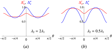
Figure 4: Angular dependence of the SC gap along the inner (red) and outer (blue) electron pocket in the case where the SOC coupling is much larger than the electron pockets mismatch. The positions of the gap minima are controlled by $\lambda_{2}/\lambda_{1}$.

Besides SOC, the inversion-symmetry breaking (ISB) at the interface of thin films also lifts the degeneracy between $s$-wave and $d$-wave in the case of FeSe thin films. In terms of the low-energy spinor states, ISB gives rise to the term Hu14 :

$$H_{\mathrm{ISB}}=\lambda_{\mathrm{ISB}}\sum_{\boldsymbol{k}}\Psi_{X}^{{\dagger}}\frac{\tau_{0}+\tau_{3}}{2}\Psi_{Y}+h.c.$$ (8)

Similarly to SOC, $\lambda_{\mathrm{ISB}}$ hybridizes the two electron pockets and favors $s$-wave over $d$-wave, lifting the degeneracy between the two states (Fig. 3b) and enhancing the $s$-wave pairing instability. As shown in the SM, the effect of ISB on the angular dependence of the gap functions around the inner and outer pockets is very similar to the effect of SOC. The only difference is that because ISB barely couples to the $d_{xy}$ orbitals, the gaps remain moderately anisotropic.

So far we considered only the zero-momentum contribution of the nematic fluctuations. In general, however, $\chi_{\mathrm{nem}}^{-1}\left(\mathbf{q}\right)=\xi_{\mathrm{nem}}^{-2}+q^{2}$. Thus, although small-momentum fluctuations do not couple the $X$ and $Y$ pockets, leaving the $s$-wave/$d$-wave degeneracy intact, large-momentum fluctuations couple them, giving rise to their own free-energy coupling $\gamma^{\prime}$ in Eq. (7). As shown in the SM, however, $\gamma^{\prime}\ll\gamma$, implying that the small-momentum approximation is sensible.

Besides SOC and ISB, other effects can lift the $s$-wave/$d$-wave degeneracy promoted by the dominant nematic fluctuations. For instance, magnetic fluctuations peaked at $(\pi,\pi)$ would favor the $d$-wave state Khodas12 ; Hinojosa15 , whereas a momentum-independent electron-phonon interaction would favor the $s$-wave state. To the best of our knowledge, no sign of $(\pi,\pi)$ magnetic order has been observed in FeSe thin films with only electron pockets. First-principle calculations for the momentum-independent phonon coupling estimate a resulting $T_{c}\lesssim 1$ K Xing14 , an energy scale that may be too small to significantly lift the degeneracy, since $T_{c}\approx 40$ K in FeSe thin films.

Previous works have shown that forward-scattering phonons can lead to a sizable enhancement of $T_{c}$ in FeSe films grown over SrTiO₃ or BaTiO₃ Lee12 ; Rademaker16 ; Johnston16 ; DHLee_STO ; Dolgov16 ; Millis16 . Indeed, the observation of replica band in ARPES measurements highlights the importance of this phonon mode Shen14 . Similarly to the nematic fluctuations studied here, forward-scattering phonons are also peaked at zero momentum, and therefore are expected to also promote degenerate $s$-wave/$d$-wave SC states Dolgov16 . In this regard, the two pairing mechanisms may cooperate to promote a robust SC state, whose degeneracy is lifted by SOC or ISB. While a detailed analysis of this problem is beyond the scope of this work, it is tempting to attribute to this cooperative effect the fact that $T_{c}$ is higher in FeSe films grown over titanium oxide interfaces as compared to other types of interfaces or other FeSe-based compounds.

Summary   In summary, we showed that the combined effect of nematic fluctuations and SOC/ISB favors an $s$-wave state in electron-doped thin films of FeSe, in agreement with recent experimental proposals FengNP15 . The role played by SOC and ISB is fundamental to lift the degeneracy with the sub-leading $d$-wave state, which suppresses the onset of long-range SC order. Although nematic fluctuations are momentum-independent in our model, the gap function can acquire a pronounced angular dependence since the nematic order parameter couples differently to $d_{xz}/d_{yz}$ and $d_{xy}$ orbitals. Interestingly, in the regime where the SOC and ISB couplings are larger than the mismatch between the electron pockets, we obtain a gap function whose angular dependence agrees qualitatively with measurements in monolayer FeSe and intercalated Li_1-x(OH)_xFeSe. More generally, our work provides an interesting framework in which superconductivity can develop in the presence of nematic fluctuations.

Supplementary Material for “Superconductivity in FeSe thin films driven by the interplay between nematic fluctuations and spin-orbit coupling”

I Superconducting gap equations

I.1 No spin-orbit coupling

The non-interacting Hamiltonian in terms of the spinors $\psi_{X,Y}$ is given by $\mathcal{H}_{0}=\sum\limits_{\boldsymbol{k},i=X,Y}\Psi_{i}^{\dagger}(\boldsymbol{k})\hat{H}_{i}(\boldsymbol{k})\Psi_{i}(\boldsymbol{k})$, with:

$$\hat{H}_{X} =\begin{pmatrix}\epsilon_{1}+\frac{\boldsymbol{K}^{2}}{2m_{1}}-a_{1}K_{x}K_{y}&-iv_{-}(\boldsymbol{K})\\ iv_{-}(\boldsymbol{K})&\epsilon_{3}+\frac{\boldsymbol{K}^{2}}{2m_{3}}-a_{3}K_{x}K_{y}\end{pmatrix}\ ,\quad\hat{H}_{Y}=\begin{pmatrix}\epsilon_{1}+\frac{\boldsymbol{K}^{2}}{2m_{1}}+a_{1}K_{x}K_{y}&-iv_{+}(\boldsymbol{K})\\ iv_{+}(\boldsymbol{K})&\epsilon_{3}+\frac{\boldsymbol{K}^{2}}{2m_{3}}+a_{3}K_{x}K_{y}\end{pmatrix}$$ (S1)

and

$$v_{\pm}(\boldsymbol{K})=v(\pm K_{x}+K_{y})+p_{1}(\pm K_{x}^{3}+K_{y}^{3})+p_{2}K_{x}K_{y}(K_{x}\pm K_{y})\ .$$ (S2)

where $(K_{x},K_{y})$ refer to the 2-Fe Brillouin zone (BZ). The parameters in the Hamiltonian $\mathcal{H}_{0}$ are taken from Table IX of Ref. Oskar . The SC gap equations are given by the Feynman diagram in Fig. S1:

$$\eta_{\alpha}\hat{M}_{\alpha}=\chi_{\mathrm{nem}}T\sum_{n,\boldsymbol{k}}\left(\hat{\lambda}^{\mathrm{nem}}\right)^{T}\hat{G}_{-k}^{T}\hat{M}_{\alpha}\hat{G}_{k}\hat{\lambda}^{\mathrm{nem}}\ .$$ (S3)

where $\hat{\lambda}$, $\hat{G}_{K}$ are $4\times 4$ matrices:

$$\hat{\lambda}^{\mathrm{nem}}=\begin{pmatrix}\hat{\lambda}_{X}^{\mathrm{nem}}&0\\ 0&\hat{\lambda}_{Y}^{\mathrm{nem}}\end{pmatrix}\ ,\quad\hat{G}_{K}=\big{(}i\omega_{n}I_{4\times 4}-H(\boldsymbol{K})\big{)}^{-1}\ \text{with }\ \hat{H}(\boldsymbol{K})=\begin{pmatrix}\hat{H}_{X}(\boldsymbol{K})&0\\ 0&\hat{H}_{Y}(\boldsymbol{K})\end{pmatrix}$$

and $\hat{\lambda}_{X}^{\mathrm{nem}}$ and $\hat{\lambda}_{X}^{\mathrm{nem}}$ are defined as in the main text. For simplicity, we introduce two parameters to describe the nematic couplings $\lambda_{1}$ and $\lambda_{2}$: $\lambda=\sqrt{\lambda_{1}^{2}+\lambda_{2}^{2}}$ and $\chi=\tan^{-1}(\lambda_{2}/\lambda_{1})$. $\hat{M}_{\alpha}$ is also a $4\times 4$ matrix with the label $\alpha$ referring to different irreducible representations of the $P4/nmm$ space group. Following Ref. Oskar , there are 6 different irreducible representations corresponding to singlet pairing at the electron pockets (namely, $A_{1g}$, $B_{2g}$, $A_{2u}$, $B_{2u}$, $E_{g}$, and $E_{u}$):

$$\hat{M}_{A_{1g}/B_{2g}}=\begin{pmatrix}\Delta_{1}\\ &\Delta_{2}\\ &&\pm\Delta_{1}\\ &&&\pm\Delta_{2}\end{pmatrix}\quad\hat{M}_{A_{2u}/B_{2u}}=\begin{pmatrix}0&\dfrac{\tau_{0}\pm\tau_{3}}{2}\\ \dfrac{\tau_{0}\pm\tau_{3}}{2}&0\end{pmatrix}\quad\hat{M}_{E_{g}^{(1)}}=\begin{pmatrix}0&\tau_{-}\\ \tau_{+}&0\end{pmatrix}$$

$$\hat{M}_{E_{g}^{(2)}}=\begin{pmatrix}0&-\tau_{+}\\ -\tau_{-}&0\end{pmatrix}\quad\hat{M}_{E_{u}^{(1)}}=\begin{pmatrix}0&0\\ 0&\tau_{1}\end{pmatrix}\quad\hat{M}_{E_{u}^{(2)}}=\begin{pmatrix}\tau_{1}&0\\ 0&0\end{pmatrix}$$ (S4)

Note that because $E_{g}$ and $E_{u}$ are two-dimensional representations, we introduced the superscripts $(1)$ and $(2)$ for the two components of the representation that give the same eigenvalue $\eta$. To compute $T_{c}$, we note that an infinitesimal pairing field $\Delta_{0}$ is renormalized by nematic fluctuations according to the diagrammatic series shown in Fig. S1:

$=$ $+$

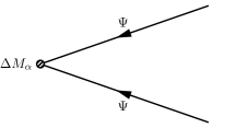
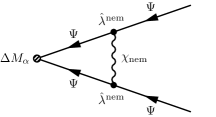
Figure S1: The effective pairing field $\Delta M_{\alpha}$ is the sum of the infinitesimal pairing field $\Delta_{0}M_{\alpha}$ and the effective pairing field dressed by nematic fluctuations.

$$\Delta\hat{M}_{\alpha}=\Delta_{0}\hat{M}_{\alpha}+\Delta\chi_{\mathrm{nem}}T\sum_{n,\boldsymbol{k}}\left(\hat{\lambda}^{\mathrm{nem}}\right)^{T}\hat{G}_{-k}^{T}\hat{M}_{\alpha}\hat{G}_{k}\hat{\lambda}^{\mathrm{nem}}\quad\Longrightarrow\quad\Delta=\frac{\Delta_{0}}{1-\eta_{\alpha}}$$ (S5)

Therefore, $T_{c}$ is obtained when the largest eigenvalue $\eta_{\alpha}(T=T_{c})=1$. In our paper, the value of the coupling $\lambda^{2}\chi_{\mathrm{nem}}$ is set such that $T_{c}=5$ meV for the case of $A_{1g}/B_{2g}$ pairing when $\lambda_{2}=0$, i.e. $\chi=0$. Fig. S2 shows the other eigenvalues $\eta_{\alpha}$ at the same temperature $T=5$ meV. Clearly, the $A_{1g}$ and $B_{1g}$ states are the degenerate leading SC instabilities of this system. The corresponding values for $\Delta_{1}$ and $\Delta_{2}$ as a function of $\chi=\tan^{-1}(\lambda_{2}/\lambda_{1})$ is also shown in the figure.

To project the gaps onto the Fermi pockets, $\Delta_{X/Y}(\boldsymbol{K})$, we introduce the spinor $u_{X/Y}\left(\mathbf{K}\right)=\big{(}u_{X/Y,1}(\boldsymbol{K}),u_{X/Y,2}(\boldsymbol{K})\big{)}^{T}$ that diagonalizes $\hat{H}_{X/Y}$ and whose eigenvalue corresponds to the band dispersion that crosses the Fermi level. Then, the projected gap is given by:

$$\Delta_{X}(\boldsymbol{K})=\Delta_{1}\big{|}u_{X,1}(\boldsymbol{K})\big{|}^{2}+\Delta_{2}\big{|}u_{X,2}(\boldsymbol{K})\big{|}^{2}$$ (S6)

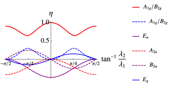
(a)

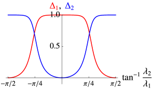
(b)

Figure S2: (a) The eigenvalues for different SC channels without SOC or ISB, as function of the ratio $\lambda_{2}/\lambda_{1}$ between the two nematic coupling constants. (b) The two intra-orbital gap functions $\Delta_{1}$ and $\Delta_{2}$ corresponding to the solution of the gap equations in the degenerate $A_{1g}$ /$B_{2g}$ channel.

I.2 Non-zero spin-orbit coupling

The SOC interaction is given by:

$$\mathcal{H}_{\mathrm{SOC}}=\frac{i}{2}\lambda_{\mathrm{SOC}}\Psi_{Y}^{{\dagger}}\left(\tau_{+}\otimes\sigma_{1}+\tau_{-}\otimes\sigma_{2}\right)\Psi_{X}+h.c.$$ (S7)

In the presence of SOC, spin-singlet and spin-triplet pairings are mixed. In general, the latter can be written as $\Psi^{T}\boldsymbol{M}\otimes i\sigma_{2}\boldsymbol{\sigma}\Psi$, where $\Psi$ is the eight-component spinor $\Psi=(\Psi_{X\sigma}\ ,\ \Psi_{Y\sigma})^{T}$. Since the spin component is symmetric for spin-triplet pairing, the orbital part $\boldsymbol{M}$ must be anti-symmetric. Since $A_{1g}$ and $B_{2g}$ are the two leading SC instabilities in the absence of SOC, we only focus on these two channels here. These irreducible representations can only be obtained if both the spin component and the orbital component transform as $E_{g}$, since $E_{g}\otimes E_{g}=A_{1g}\oplus A_{2g}\oplus B_{1g}\oplus B_{2g}$. The spin combination that transforms according to $E_{g}$ is $(i\sigma_{2}\sigma_{1},i\sigma_{2}\sigma_{2})$; for the orbital part, which must be anti-symmetric (i.e. $E_{g}^{-}$), we have:

$$-i\big{(}\Psi_{Y}^{T}\tau_{+}\Psi_{X}-\Psi_{X}^{T}\tau_{-}\Psi_{Y},\Psi_{Y}^{T}\tau_{-}\Psi_{X}-\Psi_{X}^{T}\tau_{+}\Psi_{Y}\big{)}$$ (S8)

which corresponds to inter-pocket pairing. Writing it in the form $\big{(}\Psi^{T}M_{1}\Psi,\Psi^{T}M_{2}\Psi\big{)}$, we readily obtain the non-zero matrix elements $\big{(}M_{2}\big{)}_{14}=-\big{(}M_{2}\big{)}_{41}=\big{(}M_{1}\big{)}_{23}=-\big{(}M_{1}\big{)}_{32}=i$. Combined with the spin part, we obtain the following gap functions:

$$A_{1g}: \qquad\Psi^{T}\left(\begin{pmatrix}\Delta_{1}^{A}&0&0&0\\ 0&\Delta_{2}^{A}&0&0\\ 0&0&\Delta_{1}^{A}&0\\ 0&0&0&\Delta_{2}^{A}\end{pmatrix}\otimes i\sigma_{2}+\begin{pmatrix}0&0&0&0\\ 0&0&i\Delta_{3}^{A}&0\\ 0&-i\Delta_{3}^{A}&0&0\\ 0&0&0&0\end{pmatrix}\otimes\sigma_{3}+\begin{pmatrix}0&0&0&-\Delta_{3}^{A}\\ 0&0&0&0\\ 0&0&0&0\\ \Delta_{3}^{A}&0&0&0\end{pmatrix}\otimes\sigma_{0}\right)\Psi$$ (S9)

$$B_{2g}: \qquad\Psi^{T}\left(\begin{pmatrix}\Delta_{1}^{B}&0&0&0\\ 0&\Delta_{2}^{B}&0&0\\ 0&0&-\Delta_{1}^{B}&0\\ 0&0&0&-\Delta_{2}^{B}\end{pmatrix}\otimes i\sigma_{2}+\begin{pmatrix}0&0&0&0\\ 0&0&i\Delta_{3}^{B}&0\\ 0&-i\Delta_{3}^{B}&0&0\\ 0&0&0&0\end{pmatrix}\otimes\sigma_{3}+\begin{pmatrix}0&0&0&\Delta_{3}^{B}\\ 0&0&0&0\\ 0&0&0&0\\ -\Delta_{3}^{B}&0&0&0\end{pmatrix}\otimes\sigma_{0}\right)\Psi$$ (S10)

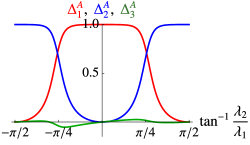
(a)

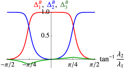
(b)

Figure S3: The solution of the $A_{1g}$ and $B_{2g}$ pairing gaps in the presence of SOC. The two nematic couplings are given by $\lambda_{1}$ and $\lambda_{2}$.

The three gaps $\Delta_{1}$, $\Delta_{2}$, and $\Delta_{3}$ are determined by solving the gap equation. In Fig. S3, we show the solution of the gap equations: clearly, the presence of spin-orbit coupling lifts the degeneracy between $A_{1g}$ and $B_{2g}$, as illustrated in Fig. 2 of the main text. Here we used $\lambda_{\mathrm{SOC}}=50$meV. We also note that the admixture with the triplet component is small.

To calculate the momentum dependence of the gap function, we project the gaps $\Delta_{1}$, $\Delta_{2}$, and $\Delta_{3}$ along the Fermi surface. Since the Hamiltonian does not break time reversal symmetry and inversion symmetry, each band is doubly degenerate (Kramers degeneracy). To show this more clearly, we define two new 4-component spinors related by time reversal symmetry:

$$\Phi_{1}=\big{(}\Psi_{X\uparrow}\quad\Psi_{Y\downarrow}\big{)}\ ,\quad\mbox{and}\quad\Phi_{2}=\big{(}\Psi_{X\downarrow}\quad-\Psi_{Y\uparrow}\big{)}$$ (S11)

Both $\mathcal{H}_{0}$ and the SOC term are diagonal in this representation:

$$\mathcal{H}_{0}+\mathcal{H}_{\mathrm{SOC}}=\sum_{\boldsymbol{K}}\Phi_{1}^{{\dagger}}\hat{H}_{1}\Phi_{1}+\sum_{\boldsymbol{K}}\Phi_{2}^{{\dagger}}\hat{H}_{2}\Phi_{2}\ ,\quad\mbox{with }\quad\hat{H}_{1}=\begin{pmatrix}\hat{H}_{X}&\hat{h}\\ \hat{h}^{{\dagger}}&\hat{H}_{Y}\end{pmatrix}\ ,\mbox{\,\ }H_{2}=\begin{pmatrix}\hat{H}_{X}&\hat{h}^{*}\\ \hat{h}^{T}&\hat{H}_{Y}\end{pmatrix}\quad,\mbox{and }\hat{h}=\frac{\lambda_{\mathrm{SOC}}}{2}\begin{pmatrix}0&-1\\ -i&0\end{pmatrix}$$

It follows immediately that $H_{1}(\boldsymbol{K})=H_{2}^{*}(-\boldsymbol{K})$. Furthermore, because the system is also invariant under inversion, the energy dispersions of $\Phi_{1}$ and $\Phi_{2}$ are exactly the same. This implies that each band in the system is doubly degenerate, although neither $\Phi_{1}$ nor $\Phi_{2}$ has degeneracies. Upon diagonalization, we find that the two overlapping electron pockets split due to the SOC, forming an inner and an outer electron pocket.

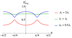
(a)

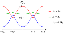
(b)

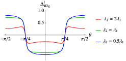
(c)

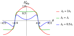
(d)

Figure S4: Projected gap on the inner ($i$) and outer ($o$) electron pockets, with $\lambda_{\mathrm{SOC}}=50$meV. (a) and (b) correspond to the $A_{1g}$ pairing channel, whereas (c) and (d) correspond to the $B_{2g}$ channel. The two nematic couplings are given by $\lambda_{1}$ and $\lambda_{2}$.

As for the pairing interaction, we find that both $A_{1g}$ and $B_{2g}$ gaps couple the two spinors, $\Phi_{1}^{T}\hat{\Delta}_{A_{1g}}\Phi_{2}$ and $\Phi_{1}^{T}\hat{\Delta}_{B_{2g}}\Phi_{2}$, with

$$\hat{\Delta}_{A_{1g}}=\begin{pmatrix}\Delta_{1}^{A}&0&0&\Delta_{3}^{A}\\ 0&\Delta_{2}^{A}&-i\Delta_{3}^{A}&0\\ 0&i\Delta_{3}^{A}&\Delta_{1}^{A}&0\\ \Delta_{3}^{A}&0&0&\Delta_{2}^{A}\end{pmatrix}\ ,\mbox{and }\quad\hat{\Delta}_{B_{2g}}=\begin{pmatrix}\Delta_{1}^{B}&0&0&-\Delta_{3}^{B}\\ 0&\Delta_{2}^{B}&-i\Delta_{3}^{B}&0\\ 0&i\Delta_{3}^{B}&-\Delta_{1}^{B}&0\\ -\Delta_{3}^{B}&0&0&-\Delta_{2}^{B}\end{pmatrix}$$

This allows us to project the gap onto the Fermi surface in a straightforward way. Consider for instance the $A_{1g}$ gap projected onto the inner Fermi pocket. We first diagonalize $H_{1}(\boldsymbol{K})$ and $H_{2}\left(\boldsymbol{K}\right)$ to obtain the band operators $u_{i,\boldsymbol{K}}$ and $v_{i,\boldsymbol{K}}$, respectively. They are related to the orbital operators $d_{\mu,\boldsymbol{K}}$ according to:

$$d_{\mu,\boldsymbol{K}} =\sum_{i}\langle\mu|u_{i}(\boldsymbol{K})\rangle u_{i,\boldsymbol{K}}$$ (S12)

$$d_{\mu,\boldsymbol{K}} =\sum_{i}\langle\mu|v_{i}(\boldsymbol{K})\rangle v_{i,\boldsymbol{K}}$$ (S13)

Due to time-reversal symmetry, $\langle\mu|v_{i}(-\boldsymbol{K})\rangle=\langle u_{i}(\boldsymbol{K})|d_{\mu}\rangle$. The SC Hamiltonian then becomes:

$$\sum_{\mu\nu}\Delta_{\mu\nu}d_{\mu,-\boldsymbol{K}}d_{\nu,\boldsymbol{K}} =\sum_{\mu\nu}\Delta_{\mu\nu}\sum_{ij}\langle\mu|v_{i}(-\boldsymbol{K})\rangle\langle\nu|u_{j}(\boldsymbol{K})\rangle v_{i,-\boldsymbol{K}}u_{j,\boldsymbol{K}}$$

$$=\sum_{\mu\nu}\Delta_{\mu\nu}\sum_{ij}\langle u_{i}(\boldsymbol{K})|\mu\rangle\langle\nu|u_{j}(\boldsymbol{K})\rangle v_{i,-\boldsymbol{K}}u_{j,\boldsymbol{K}}$$ (S14)

Projecting onto band $l$, we find:

$$\sum_{\mu\nu}\Delta_{\mu\nu}\langle u_{l}(\boldsymbol{K})|\mu\rangle\langle\nu|u_{l}(\boldsymbol{K})\rangle v_{l}(-\boldsymbol{K})u_{l}(\boldsymbol{K})=\langle u_{l}(\boldsymbol{K})|\hat{\Delta}|u_{l}(\boldsymbol{K})\rangle v_{l}(-\boldsymbol{K})u_{l}(\boldsymbol{K})$$ (S15)

As a result, the gap along the pocket corresponding to band $l$ given by:

$$\Delta_{l}\left(\boldsymbol{K}\right)=\langle u_{l}(\boldsymbol{K})|\hat{\Delta}|u_{l}(\boldsymbol{K})\rangle\ ,$$ (S16)

yielding the results shown in Fig. S4.

I.3 Inversion symmetry-breaking

As discussed in the main text, the inversion symmetry is broken at the interface of thin films of FeSe. Considering the generators of the $P4/nmm$ group, $\{\sigma_{z}|\frac{1}{2}\frac{1}{2}\}$ is the only symmetry transformation broken, as it corresponds to a reflection $\sigma_{z}$ with respect to the Fe plane followed by a translation by $\left(\frac{1}{2},\frac{1}{2}\right)$ in the 2-Fe unit cell. Because the term:

$$H_{\mathrm{ISB}}=\lambda_{\mathrm{ISB}}\Psi_{X}^{\dagger}\frac{\tau_{0}+\tau_{3}}{2}\Psi_{Y}+h.c.$$ (S17)

acquires a minus sign upon the symmetry transformation $\{\sigma_{z}|\frac{1}{2}\frac{1}{2}\}$, it must be generated once inversion symmetry is broken. Similarly to the SOC term, the ISB term hybridizes the $X$ and $Y$ pockets, and splits the degeneracy between the $A_{1g}$ and $B_{2g}$ pairing states. Unlike the SOC case, there is no admixture with triplet components. However, to solve the gap equations, one needs to introduce an admixture with the pairing channel $A_{2u}$, resulting in the pairing matrix of the form:

$$\hat{M}_{A_{1g}+A_{2u}}=\begin{pmatrix}\Delta_{1}&0&\Delta_{3}&0\\ 0&\Delta_{2}&0&0\\ \Delta_{3}&0&\Delta_{1}&0\\ 0&0&0&\Delta_{2}\end{pmatrix}$$ (S18)

In Fig. S5, we show the solution of the gap equations and the corresponding gap functions projected onto the Fermi surface.

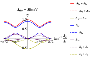
(a)

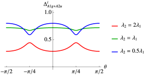
(b)

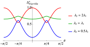
(c)

Figure S5: (a) The SC eigenvalue $\eta$ in different SC channels for $\lambda_{\mathrm{ISB}}=50$meV. (b) and (c): Projected gap on the inner ($i$) and outer ($o$) electron pockets in the leading $A_{1g}+A_{2u}$ pairing channel. The two nematic couplings are given by $\lambda_{1}$ and $\lambda_{2}$.

II Superconducting free energy

II.1 No spin-orbit coupling

In the absence of SOC and ISB, the $s$-wave and $d$-wave channels have the same $T_{c}$. In terms of a free energy expansion, this implies that, to quadratic order in the gaps:

$$F^{(2)}=\alpha\left(|\Delta_{s}|^{2}+|\Delta_{d}|^{2}\right)$$ (S19)

In this section we study how this degeneracy is affected by quartic coefficients in the free energy, which go beyond the linearized SC gap equations. For notation convenience, we define the superconducting order parameters $\Delta_{s}$ and $\Delta_{d}$ by

$$\hat{\Delta}_{A_{1g}}=\Delta_{s}\begin{pmatrix}\cos\alpha_{s}&0&0&0\\ 0&\sin\alpha_{s}&0&0\\ 0&0&\cos\alpha_{s}&0\\ 0&0&0&\sin\alpha_{s}\end{pmatrix}\otimes i\sigma_{2}\qquad\hat{\Delta}_{B_{2g}}=\Delta_{d}\begin{pmatrix}\cos\alpha_{d}&0&0&0\\ 0&\sin\alpha_{d}&0&0\\ 0&0&-\cos\alpha_{d}&0\\ 0&0&0&-\sin\alpha_{d}\end{pmatrix}\otimes i\sigma_{2}\ .$$

They are related to the gaps $\Delta_{1,2}^{A/B}$ according to $\Delta_{1}^{A/B}=\Delta_{s/d}\cos\alpha_{s/d}$ and $\Delta_{2}^{A/B}=\Delta_{s/d}\sin\alpha_{s/d}$. The parameters $\alpha_{s/d}$ are obtained from the gap equations. The quartic terms of the free energy are given by:

$$F^{(4)}=\frac{T}{2}\sum_{k}\mathrm{Tr}\Big{(}\hat{G}_{k}\hat{\Delta}\hat{G}_{-k}^{T}\hat{\Delta}^{\dagger}\hat{G}_{k}\hat{\Delta}\hat{G}_{-k}^{T}\hat{\Delta}^{\dagger}\Big{)}\ ,\quad\text{with }\quad\hat{\Delta}=\hat{\Delta}_{A_{1g}}+\hat{\Delta}_{B_{2g}}\ .$$

yielding:

$$F^{(4)}=\beta_{1}|\Delta_{d}|^{4}+\gamma_{1}|\Delta_{s}|^{2}|\Delta_{d}|^{2}+\frac{\gamma_{2}}{2}\left(\Delta_{s}^{*2}\Delta_{d}^{2}+c.c.\right)+\beta_{2}|\Delta_{d}|^{4}\ ,$$ (S20)

Evaluating the trace gives $\gamma_{1}=2\gamma_{2}=4\beta_{1}=4\beta_{2}=4\beta$. Thus, the free energy can be written as

$$F=\alpha\left(|\Delta_{s}|^{2}+|\Delta_{d}|^{2}\right)+\beta\left(|\Delta_{s}|^{4}+|\Delta_{d}|^{4}+4|\Delta_{s}|^{2}|\Delta_{d}|^{2}+\Delta_{s}\Delta_{d}^{*}+\Delta_{s}^{*}\Delta_{d}\right)$$ (S21)

Minimizing the free energy with respect to the relative phase between $\Delta_{s}$ and $\Delta_{d}$ give $\pi/2$. Under this condition, the free energy is given by:

$$F=\alpha\left(|\Delta_{s}|^{2}+|\Delta_{d}|^{2}\right)+\beta\left(|\Delta_{s}|^{2}+|\Delta_{d}|^{2}\right)^{2}$$ (S22)

Thus, besides the $U(1)$ symmetry related to the global phase, there is an additional $U(1)$ symmetry related to the fact that only the value of $|\Delta_{s}|^{2}+|\Delta_{d}|^{2}$ is fixed by minimization of the free energy. Equivalently, we can write the $s$ and $d$ gaps in terms of the gaps on the two electron pockets, $\Delta_{X}$ and $\Delta_{Y}$. To see this, we note that the solution of the gap equations for the $s$ and $d$ gaps give the same parameter $\alpha_{s}=\alpha_{d}$. Then the total gap can be written as:

$$\hat{\Delta}=\hat{\Delta}_{A_{1g}}+\hat{\Delta}_{B_{2g}}=\left(\begin{array}[]{cc}\left(\Delta_{s}+\Delta_{d}\right)\tilde{\tau}&0\\ 0&\left(\Delta_{s}-\Delta_{d}\right)\tilde{\tau}\end{array}\right)$$ (S23)

with the $2\times 2$ diagonal matrix $\tilde{\tau}=\mathrm{diag}\left(\cos\alpha_{s},\,\sin\alpha_{s}\right)$. Since the upper (lower) diagonal block is related to the $X$ ($Y$) pocket, we have:

$$\Delta_{X} =\Delta_{s}+\Delta_{d}\ ,\qquad\Delta_{Y}=\Delta_{s}-\Delta_{d}$$

Substitution in the free energy yields two decoupled superconducting systems:

$$F=\frac{\alpha}{2}\left(|\Delta_{X}|^{2}+|\Delta_{Y}|^{2}\right)+\frac{\beta}{2}\left(\big{|}\Delta_{X}\big{|}^{4}+\big{|}\Delta_{Y}\big{|}^{4}\right)$$ (S24)

II.2 Non-zero spin-orbit coupling and inversion symmetry-breaking

The main effect of the SOC (and also of the ISB) is to generate a quadratic coupling between the two gaps $\Delta_{X}$ and $\Delta_{Y}$. According to the Feynman diagram of Fig. 3 in the main text, these terms generate the quadratic contribution to the free energy:

$$\delta F=\gamma\left(\Delta_{X}\Delta_{Y}^{*}+\Delta_{X}^{*}\Delta_{Y}\right)$$ (S25)

Here we illustrate the computation of $\gamma$ for the case of SOC. The Feynman diagram gives:

$$\gamma= -\left(\frac{i\lambda}{2}\right)^{2}T\sum_{n,\boldsymbol{k}}\mathrm{Tr}\left[\Delta_{X}\otimes i\sigma_{2}G_{X}(\omega_{n},\boldsymbol{K})\big{(}\tau_{+}\otimes\sigma_{1}+\tau_{-}\otimes\sigma_{2}\big{)}G_{Y}(\omega_{n},\boldsymbol{K})\Delta_{Y}^{*}\otimes(-i\sigma_{2})G_{Y}^{T}(-\omega_{n},-\boldsymbol{K})\right.$$

$$\qquad\left.\big{(}\tau_{+}\otimes\sigma_{1}+\tau_{-}\otimes\sigma_{2}\big{)}^{T}G_{X}^{T}(-\omega_{n},-\boldsymbol{K})\right]$$

$$= -\frac{\lambda^{2}}{2}T\sum_{n,\boldsymbol{k}}\left\{\left(G_{Y}\Delta_{Y}^{*}G_{Y}^{T}\right)_{22}\left(G_{X}^{T}\Delta_{X}G_{X}\right)_{11}+\left(G_{Y}\Delta_{Y}^{*}G_{Y}^{T}\right)_{11}\left(G_{X}^{T}\Delta_{X}G_{X}\right)_{22}\right\}$$ (S26)

where $G_{X/Y}=(i\omega_{n}-H_{X/Y}(K))^{-1}$ and $G_{X/Y}^{T}=(-i\omega_{n}-H_{X/Y}^{T}(-\boldsymbol{K}))^{-1}$. In general, the diagonal component of $G_{X}^{T}\Delta_{X}G_{X}$ could be either positive or negative. But if we only focus on the projection along the band that crosses the Fermi level, this diagonal component must be positive. Consider for instance the wave-function $|u(\boldsymbol{K})\rangle$ that diagonalizes $H_{X}(\boldsymbol{K})$ and gives the band $\epsilon_{u}(\boldsymbol{K})$ that crosses the Fermi surface. We find:

$$\left(G_{X}^{T}\Delta_{X}G_{X}\right)_{ii}\approx\frac{\langle u(\boldsymbol{K})|\Delta_{X}|u(\boldsymbol{K})\rangle\left|\langle i|u(\boldsymbol{K})\rangle\right|^{2}}{(-i\omega_{n}-\epsilon_{u}(\boldsymbol{K}))(i\omega_{n}-\epsilon_{u}(\boldsymbol{K}))}=\frac{\left|\langle i|u(\boldsymbol{K})\rangle\right|^{2}}{\omega_{n}^{2}+\epsilon_{u}^{2}(\boldsymbol{K})}\langle u(\boldsymbol{K})|\Delta_{X}|u(\boldsymbol{K})\rangle$$ (S27)

Since:

$$\langle u(\boldsymbol{k})|\Delta_{X}|u(\boldsymbol{k})\rangle=\Delta_{1}|u_{1}(\boldsymbol{k})|^{2}+\Delta_{2}|u_{2}(\boldsymbol{k})|^{2}$$

is the SC gap projected onto the band that crosses the Fermi level, we find that it is always positive, because both $\Delta_{1}$ and $\Delta_{2}$ are positive, as shown in Fig. S2. Thus, it follows that $\gamma<0$.

As for the quartic coefficients, we find that in the presence of SOC or ISB they satisfy the relationship $\gamma_{1}-\gamma_{2}\lessapprox 2\sqrt{\beta_{1}\beta_{2}}$. As a result, the two gap functions can in principle coexist and break time reversal symmetry at low temperatures.

II.3 Large-momentum nematic fluctuations

In the previous subsection, we investigated the effect of SOC and ISB in lifting the $s$-wave/$d$-wave degeneracy. It is interesting to study whether large-momentum nematic fluctuations, involving momentum transfer $\boldsymbol{q}\approx M=(\pi,\pi)$ and thus coupling the electron pockets, give rise to a similar effect. We note that these large-momentum fluctuations are actually associated with orbital order that breaks translational symmetry (antiferro-orbital order), instead of ferro-orbital order. The fact that the associated antiferro-orbital order has not been observed in bulk or thin films of FeSe suggests that these fluctuations are much smaller than the nematic ones, and therefore can be considered a perturbation on top of the superconducting state obtained previously. For this reason, the main contribution of the large-momentum nematic fluctuations $\chi_{M}$ to the superconducting free energy is captured by the Feynman diagram in Fig. S6, yielding the quadratic term:

Figure S6: Feynman diagram representing the coupling between the gaps in the two electron pockets mediated by large-momentum nematic fluctuations $\chi_{nem}(\boldsymbol{q}\approx\boldsymbol{M})\equiv\chi_{M}$. Similar to SOC, this coupling also lifts the degeneracy between s-wave and d-wave, but with a much smaller effect.

$$\delta F=\gamma^{\prime}(\Delta_{X}^{*}\Delta_{Y}+\Delta_{Y}^{*}\Delta_{X})$$ (S28)

with

$$\gamma^{\prime}= -T^{2}\sum_{m,n}\int\frac{{\rm d}^{2}\boldsymbol{k}}{(2\pi)^{2}}\frac{{\rm d}^{2}\boldsymbol{k}^{\prime}}{(2\pi)^{2}}\frac{\lambda^{2}\chi(\omega_{n}-\omega_{m},\boldsymbol{k}-\boldsymbol{k}^{\prime}+\boldsymbol{M})}{(i\omega_{n}-\epsilon_{X}(\boldsymbol{k}))(-i\omega_{n}-\epsilon_{X}(-\boldsymbol{k}))(i\omega_{m}-\epsilon_{Y}(\boldsymbol{k}^{\prime}))(-i\omega_{m}-\epsilon_{Y}(-\boldsymbol{k}^{\prime}))}$$

$$\approx -\lambda^{2}\chi_{M}T^{2}\sum_{m,n}\int\frac{{\rm d}^{2}\boldsymbol{k}}{(2\pi)^{2}}\frac{{\rm d}^{2}\boldsymbol{k}^{\prime}}{(2\pi)^{2}}\frac{1}{(\omega_{n}^{2}+\epsilon_{X}^{2}(\boldsymbol{k}))(\omega_{m}^{2}+\epsilon_{Y}^{2}(\boldsymbol{k}^{\prime}))}$$

$$\approx -N_{f}^{2}\lambda^{2}\chi_{M}\left(\ln\frac{\Lambda}{T_{c}}\right)^{2}$$ (S29)

In the above formula, we made the approximation that the nematic susceptibility is peaked at zero frequency and momentum $\mathbf{Q}$, and neglected the orbital dependence of the coupling between the fermions and the nematic fluctuation. It is obvious that $\gamma^{\prime}<0$, showing that the nematic fluctuation $\chi_{M}$ also favors $s$ wave.

Next, we compare the effects of large-momentum fluctuations and SOC in lifting the degeneracy by comparing $\gamma^{\prime}$ calculated here with $\gamma$ calculated in Eq. (S25). From Fig. 3, we can estimate $\gamma$ as:

$$\gamma\approx-T\sum_{n}\int\frac{{\rm d}^{2}\boldsymbol{k}}{(2\pi)^{2}}\frac{\lambda_{SOC}^{2}}{(\omega_{n}^{2}+\epsilon_{x}^{2}(\boldsymbol{k}))(\omega_{n}^{2}+\epsilon_{y}^{2}(\boldsymbol{k}))}\approx-\lambda_{SOC}^{2}T\sum_{n}\int\frac{{\rm d}^{2}\boldsymbol{k}}{(2\pi)^{2}}\frac{1}{(\omega_{n}^{2}+\epsilon^{2}(\boldsymbol{k}))^{2}}\sim-N_{f}\frac{\lambda_{SOC}^{2}}{T_{c}^{2}}$$

Furthermore, we can use for $T_{c}$:

$$\ln\frac{\Lambda}{T_{c}}\approx\frac{1}{N_{f}\lambda^{2}\chi_{0}}$$ (S30)

where $\chi_{0}$ is the zero-momentum nematic susceptibility. Substituting in the equations above, we find:

$$\frac{\gamma}{\gamma^{\prime}}=\frac{\chi_{0}}{\chi_{M}}\frac{\lambda_{SOC}^{2}}{T_{c}^{2}}\left(\ln\frac{\Lambda}{T_{c}}\right)^{-1}\approx\left(1+2\pi^{2}\xi_{\mathrm{nem}}^{2}a^{-2}\right)\frac{\lambda_{SOC}^{2}}{T_{c}^{2}}\left(\ln\frac{\Lambda}{T_{c}}\right)^{-1}$$ (S31)

where, in the last step, we considered the expansion $\chi_{\mathrm{nem}}^{-1}(\mathbf{q})=\xi_{\mathrm{nem}}^{-2}+q^{2}$ and substituted $\chi_{0}=\chi_{\mathrm{nem}}(0)$, $\chi_{0}=\chi_{\mathrm{nem}}(\pi,\pi)$. We now substitute reasonable, experimentally-based values for these quantities. According to ARPES data in bulk FeSe Zhigadlo16S , $\lambda_{SOC}\approx 10$ meV, which is of the same order as $T_{c}\approx 6$ meV of the thin films. The bandwidth can be estimated as $\Lambda\sim 100$ meV, whereas the nematic correlation length is certainly a few lattice constants – say $\xi=5a$. Substituting these numbers, we estimate $\gamma/\gamma^{\prime}\approx 500\gg 1$. Therefore, the effect of large-momentum fluctuations is negligible compared to the effect of spin-orbit coupling. A similar analysis for the inversion symmetry-breaking contribution reveals the latter is also much larger than the large-momentum fluctuations contribution, as long as $\lambda_{ISB}>1$ meV. Although this is a reasonable value, first principle calculations are necessary to estimate $\lambda_{ISB}$, which is beyond the scope of this paper.

III Fermi-surface projected Model

In the previous analyses, we considered the low-energy model derived directly from the $5\times 5$ tight-binding Hamiltonian. To gain more insight into the problem, we can further restrict our analysis only to the bands that cross the Fermi level, since they give the dominant contribution to the pairing instability. It is then convenient to write the $X$ and $Y$ pockets dispersions (here $\boldsymbol{k}$ refers to the 1-Fe unit cell):

$$\varepsilon_{X,\mathbf{k}}=\frac{k^{2}}{2m}-\epsilon_{\mu}-\epsilon_{m}\cos 2\theta\ ,\varepsilon_{Y,\mathbf{k}}=\frac{k^{2}}{2m}-\epsilon_{\mu}+\epsilon_{m}\cos 2\theta$$ (S32)

and the non-interacting Hamiltonian in terms of the band operators $f_{X}$ and $f_{Y}$:

$$H_{0}=\sum_{\boldsymbol{k}}\varepsilon_{X,\boldsymbol{k}}f_{X,\mathbf{k}}^{\dagger}f_{X,\mathbf{k}}^{\phantom{\dagger}}+\sum_{\boldsymbol{k}}\varepsilon_{Y,\boldsymbol{k}}f_{Y,\mathbf{k}}^{\dagger}f_{Y,\mathbf{k}}^{\phantom{\dagger}}$$ (S33)

Here, $\epsilon_{m}$ gives the mismatch between the two electron pockets. The advantage of this model over the previous one is that it allows us to easily tune the ratio between the mismatch and the SOC, $\epsilon_{m}/\lambda_{\mathrm{SOC}}$, which in the full model above is fixed by the parameter $v$ in Eq. S1. To proceed, we write down the relationship between the band operators $f_{X}$, $f^{\prime}_{X}$ and the orbital operators $d_{xy},\,d_{yz}$ Fernandes14 :

$$f_{X}\left(\theta\right)=\frac{\alpha d_{xy}+i\sin\theta d_{yz}}{\sqrt{\alpha^{2}+\sin^{2}\theta}}\ ;\quad f^{\prime}_{X}\left(\theta\right)=\frac{i\sin\theta d_{xy}+\alpha d_{yz}}{\sqrt{\alpha^{2}+\sin^{2}\theta}}\ .$$ (S34)

where $\theta$ is the polar angle. The factor $i$ is inserted to keep the wave-function time-reversal invariant. While $f_{X}$ describes the band obtained from the diagonalization of $\hat{H}_{X}$ that crosses the Fermi level, $f^{\prime}_{X}$ describes the band that do not cross the Fermi level. These relationships can be inverted to give:

$$d_{xy}=\frac{\alpha f_{X}-i\sin\theta f^{\prime}_{X}}{\sqrt{\alpha^{2}+\sin^{2}\theta}}\ ,\qquad d_{yz}=\frac{-i\sin\theta f_{X}+\alpha f^{\prime}_{X}}{\sqrt{\alpha^{2}+\sin^{2}\theta}}\ .$$ (S35)

The band operators $f_{Y}$, $f^{\prime}_{Y}$, related to the $Y$ pocket, are obtained by a rotation of $\pi/2$ followed by a mirror reflection $\sigma_{z}$ with respect to the $(x,y)$ plane:

$$\theta\rightarrow\theta-\frac{\pi}{2}\ ,\quad d_{xy}\rightarrow-d_{xy}\ ,\quad d_{yz}\rightarrow d_{xz}\quad\Longrightarrow\quad f_{Y}\left(\theta\right)=-\frac{\alpha d_{xy}+i\cos\theta d_{xz}}{\sqrt{\alpha^{2}+\cos^{2}\theta}}\ ;\quad f^{\prime}_{Y}\left(\theta\right)=\frac{i\cos\theta d_{xy}+\alpha d_{xz}}{\sqrt{\alpha^{2}+\cos^{2}\theta}}\ .$$

The coupling between nematic fluctuations and the band operators associated with the $X$ electron pocket can be obtained from:

$$H_{\mathrm{int},X} =\lambda\sum_{\mathbf{k},\mathbf{k}^{\prime}}\phi_{\mathbf{k}-\mathbf{k}^{\prime}}\left(\cos\chi d_{yz,\mathbf{k}^{\prime}}^{\dagger}d_{yz,\mathbf{k}}+\sin\chi d_{xy,\mathbf{k}^{\prime}}^{\dagger}d_{xy,\mathbf{k}}\right)$$ (S36)

$$H_{\mathrm{int},X} =\lambda\sum_{\mathbf{k},\mathbf{k}^{\prime}}\phi_{\mathbf{k}-\mathbf{k}^{\prime}}\left(\frac{\alpha^{2}\sin\chi+\cos\chi\sin\theta\sin\theta^{\prime}}{\sqrt{\big{(}\alpha^{2}+\sin^{2}\theta^{\prime}\big{)}\big{(}\alpha^{2}+\sin^{2}\theta\big{)}}}\right)f_{X}^{\dagger}(\theta^{\prime})f_{X}(\theta)$$ (S37)

where $\chi=\tan^{-1}\big{(}\lambda_{2}/\lambda_{1}\big{)}$ and $\lambda=\sqrt{\lambda_{1}^{2}+\lambda_{2}^{2}}$ are related to the two nematic couplings $\lambda_{1}$ and $\lambda_{2}$. Since we are interested on the states at the Fermi level, we hereafter focus only on the contributions arising from bilinear combinations of $f_{X}$ and $f_{Y}$, since the band dispersions corresponding to $f^{\prime}_{X}$ and $f^{\prime}_{Y}$ do not cross the Fermi surface. Similarly, for pocket $Y$ we find:

$$H_{\mathrm{int},Y}=-\lambda\sum_{\mathbf{k},\mathbf{k}^{\prime}}\phi_{\mathbf{k}-\mathbf{k}^{\prime}}\left(\frac{\alpha^{2}\sin\chi+\cos\chi\cos\theta\cos\theta^{\prime}}{\sqrt{\big{(}\alpha^{2}+\cos^{2}\theta^{\prime}\big{)}\big{(}\alpha^{2}+\cos^{2}\theta\big{)}}}\right)f_{Y}^{\dagger}(\theta^{\prime})f_{Y}(\theta)$$ (S38)

The linearized gap equations for the two pockets then become:

$$\eta\Delta_{X}(\theta) =\lambda^{2}\chi_{\mathrm{nem}}N_{0}\ln\frac{\Lambda}{T}\int\frac{{\rm d}\theta^{\prime}}{2\pi}\frac{\left(\alpha^{2}\sin\chi+\cos\chi\sin\theta\sin\theta^{\prime}\right)^{2}}{\big{(}\alpha^{2}+\sin^{2}\theta^{\prime}\big{)}\big{(}\alpha^{2}+\sin^{2}\theta\big{)}}\Delta_{X}(\theta^{\prime})\ ,$$ (S39)

$$\eta\Delta_{Y}(\theta) =\lambda^{2}\chi_{\mathrm{nem}}N_{0}\ln\frac{\Lambda}{T}\int\frac{{\rm d}\theta^{\prime}}{2\pi}\frac{\left(\alpha^{2}\sin\chi+\cos\chi\cos\theta\cos\theta^{\prime}\right)^{2}}{\big{(}\alpha^{2}+\cos^{2}\theta^{\prime}\big{)}\big{(}\alpha^{2}+\cos^{2}\theta\big{)}}\Delta_{Y}(\theta^{\prime})\ ,$$ (S40)

where $\Lambda$ is the high energy cutoff, and $N_{0}$ is the density of states. These gap equations can be conveniently parametrized and solved in terms of the intra-orbital gaps $\Delta_{1}$ and $\Delta_{2}$:

$$\Delta_{X}\left(\theta\right) =\frac{\Delta_{1}\alpha^{2}+\Delta_{2}\sin^{2}\theta}{\alpha^{2}+\sin^{2}\theta}$$ (S41)

$$\Delta_{Y}\left(\theta\right) =\frac{\Delta_{1}\alpha^{2}+\Delta_{2}\cos^{2}\theta}{\alpha^{2}+\cos^{2}\theta}$$ (S42)

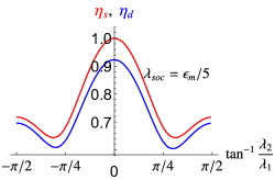
(a)

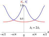
(b)

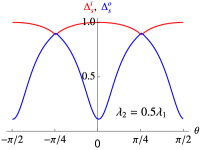
(c)

Figure S7: SC in different channels for $\alpha=0.5$ and $\lambda_{\mathrm{SOC}}=5\epsilon_{m}$. (a) The eigenvalues of the $A_{1g}$ ($s$-wave) and $B_{2g}$ ($d$-wave) pairing channels. (b) and (c): Projected gap functions of the $A_{1g}$ solution onto the inner and outer electron pockets for $\lambda_{2}=2\lambda_{1}$ and $\lambda_{2}=0.5\lambda_{1}$, respectively.

To calculate the gap function in the presence of SOC and ISB, we need to write down the two additional non-interacting terms in the band basis. The SOC is given by

$$H_{\mathrm{SOC}}=\frac{i}{2}\lambda_{\mathrm{SOC}}\sum_{\boldsymbol{k}}\left[d_{xz,\boldsymbol{k}+\boldsymbol{Q}_{Y}}^{\dagger}\sigma_{1}d_{xy,\boldsymbol{k}+\boldsymbol{Q}_{X}}+d_{xy,\boldsymbol{k}+\boldsymbol{Q}_{Y}}^{{\dagger}}\sigma_{2}d_{yz,\boldsymbol{k}+\boldsymbol{Q}_{X}}\right]+h.c.$$ (S43)

Projecting onto the Fermi surface, we find:

$$H_{\mathrm{SOC}}=\lambda_{\mathrm{SOC}}\sum_{\boldsymbol{k}}\frac{\alpha}{2\sqrt{\alpha^{2}+\cos^{2}\theta}\sqrt{\alpha^{2}+\sin^{2}\theta}}f_{Y}^{{\dagger}}\left(\cos\theta\sigma_{1}-\sin\theta\sigma_{2}\right)f_{X}+h.c.$$ (S44)

Similarly, the ISB term is:

$$H_{\mathrm{ISB}}=\lambda_{\mathrm{ISB}}\sum_{\boldsymbol{k}}d_{xz,\boldsymbol{k}+\boldsymbol{Q}_{Y}}^{\dagger}d_{yz,\boldsymbol{k}+\boldsymbol{Q}_{X}}+h.c.$$ (S45)

whose projection onto the Fermi surface gives:

$$H_{\mathrm{ISB}}=-\lambda_{\mathrm{ISB}}\sum_{\boldsymbol{k}}\frac{\sin\theta\cos\theta}{\sqrt{\alpha^{2}+\cos^{2}\theta}\sqrt{\alpha^{2}+\sin^{2}\theta}}\,f_{X}^{\dagger}f_{Y}+h.c.\$$ (S46)

The results for the case of SOC are shown in Fig. S7 (for $\lambda_{\mathrm{SOC}}\ll\epsilon_{m}$) and S8 (for $\lambda_{\mathrm{SOC}}\gg\epsilon_{m}$). In the former case, the angular dependence of the gap functions in the inner and outer pockets, and the splitting of the $A_{1g}$ and $B_{2g}$ degeneracies, are similar to Fig. 2 of the main text, which was obtained using the full orbital model. In the latter case, the degeneracy lifting is more pronounced, and the gaps in the two pockets are similar, as shown in Fig. 4 of the main text.

Figure S8: Eigenvalues of the $A_{1g}$ ($s$-wave) and $B_{2g}$ ($d$-wave) pairing channels for $\alpha=0.5$ and $\lambda_{\mathrm{SOC}}=5\epsilon_{m}$.

The impact of ISB on SC is similar to the case of SOC. As shown in Fig. S9 (for $\lambda_{\mathrm{ISB}}\gg\epsilon_{m}$), the $A_{1g}+A_{2u}$ ($s$-wave) pairing is the leading instability. The angular dependence of the SC gap is also similar to the case of large SOC. The sharp peaks or troughs at $\theta=0$ and $\pm\pi/2$ are a consequence of the fact that the effective ISB term $\lambda_{\mathrm{ISB}}$ vanishes at these points of the Fermi surface.

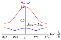
(a)

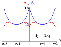
(b)

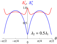
(c)

Figure S9: SC in different channels for $\alpha=0.5$ and $\lambda_{\mathrm{ISB}}=5\epsilon_{m}$. (a) The eigenvalues of the $A_{1g}+A_{2u}$ ($s$-wave) and $B_{2g}$ ($d$-wave) pairing channels. (b) and (c): Projected gap functions of the $A_{1g}+A_{2u}$ solution onto the inner and outer electron pockets for $\lambda_{2}=2\lambda_{1}$ and $\lambda_{2}=0.5\lambda_{1}$, respectively.

References

(1) I. I. Mazin, D. J. Singh, M. D. Johannes, M.H.
Du, Phys. Rev. Lett. 101, 057003 (2008).
(2) P. J. Hirschfeld, M. M. Korshunov, and I.
I. Mazin, Rep. Prog. Phys. 74, 124508 (2011).
(3) D. N. Basov and A. V. Chubukov, Nature Phys.
7, 272 (2011).
(4) A. V. Chubukov, Annu. Rev. Condens. Matter
Phys. 3, 5792 (2012).
(5) Q. Y. Wang, et al., Chin. Phys. Lett. 29,
037402 (2012).
(6) D. F. Liu et al., Nat. Commun. 3,
931 (2012).
(7) S. L. He et al., Nat. Mater. 12,
605 (2013).
(8) S. Tan et al., Nat. Mater. 12, 634
(2013).
(9) W. H. Zhang, et al., Chin. Phys. Lett. 31,
017401 (2014).
(10) J.-F. Ge, Z.-L. Liu, C. Liu, C.-L. Gao, D. Qian,
Q.-K. Xue, Y. Liu, and J.-F. Jia, Nature Mater., 14, 285
(2014).
(11) P. Zhang, et al., Phys. Rev. B 94,
104510 (2016).
(12) R. Peng, et al., Nature Commun. 5,
5044 (2014).
(13) B. Lei, et al., Phys. Rev. Lett. 116,
077002 (2016).
(14) Y. Sun, W. Zhang, Y. Xing, F. Li, Y. Zhao, Z. Xia,
L. Wang, X. Ma, Q.-K. Xue, and J. Wang, Sci. Rep. 4, 6040
(2014).
(15) E. Pomjakushina, K. Conder, V. Pomjakushin,
M. Bendele, and R. Khasanov, Phys. Rev. B 80, 024517 (2009).
(16) J. J. Lee, et al., Nature 515, 245
(2014).
(17) F.-C. Hsu, et al., Proc. Natl Acad. Sci. 105
14262 (2008).
(18) Y.-Y. Xiang, F. Wang, D. Wang, Q.-H. Wang, and D.-H.
Lee, Phys. Rev. B 86, 134508 (2012).
(19) Y. C. Tian, W. H. Zhang, F. S. Li, Y. L. Wu, Q.
Wu, F. Sun, G. Y. Zhou, L. Wang, X. Ma, Q.-K. Xue, and J. Zhao, Phys.
Rev. Lett. 116, 107001 (2016).
(20) L. Rademaker, Y. Wang, T. Berlijn, and S. Johnston,
New J. Phys. 18, 022001 (2016).
(21) Y. Zhou and A. J. Millis, Phys. Rev. B 93,
224506 (2016).
(22) Z.-X. Li, F. Wang, H. Yao, and D. H. Lee, Science
Bulletin 61, 925 (2016).
(23) Y. Wang, K. Nakatsukasa, L. Rademaker, T. Berlijn,
and S. Johnston, Supercond. Sci. Technol. 29, 054009 (2016).
(24) M. L. Kulic and O. V. Dolgov, arXiv:1607.00843.
(25) J. Shiogai, Y. Ito, T. Mitsuhashi, T. Nojima,
and A. Tsukazaki, Nature Phys. 12 42 (2016).
(26) Z. R. Ye, et al., arXiv:1512.02526.
(27) Y. Miyata, K. Nakayama, K. Sugawara, T. Sato,
and T. Takahashi, Nature Mater. 14, 775 (2015).
(28) X. H. Niu, et al., Phys. Rev. B 92, 060504
(2015).
(29) L. Zhao, et al., Nat. Commun. 7,
10608 (2016).
(30) M. D. Watson, et al., Phys. Rev. B 91,
155106 (2015).
(31) A. V. Chubukov, R. M. Fernandes, and J. Schmalian,
Phys. Rev. B 91, 201105 (2015).
(32) A. V. Chubukov, M. Khodas, and R. M. Fernandes, arXiv:1602.05503.
(33) F. Wang, S. A. Kivelson, and D.-H. Lee, Nature
Phys. 11, 959 (2015).
(34) R. Yu and Q. Si, Phys. Rev. Lett. 115, 116401
(2015).
(35) J. K. Glasbrenner, I. I. Mazin, H. O. Jeschke,
P. J. Hirschfeld, R. M. Fernandes, and R. Valenti, Nature Phys. 11,
953 (2015).
(36) Y. Zhang, et al., Phys. Rev. B 94,
115153 (2016).
(37) C. H. P. Wen, et al., Nat. Commun. 7
10840 (2016).
(38) D. Huang, T. A. Webb, S. Fang, C.-L. Song, C.-Z.
Chang, J. S. Moodera, E. Kaxiras, and J. E. Hoffman, Phys. Rev. B
93, 125129 (2016).
(39) H. Yamase and R. Zeyher, Phys. Rev. B 88,
180502(R) (2013).
(40) P. T. Dumitrescu, M. Serbyn, R. T. Scalettar,
and A. Vishwanath, Phys. Rev. B 94, 155127 (2016).
(41) S. V. Borisenko, et al., Nat. Phys. 12
311 (2016).
(42) Q. Fan et al., Nature Phys. 11,
946 (2015).
(43) R. Peng, et al., Phys. Rev. Lett. 112,
107001 (2014).
(44) Z. Du, X. Yang, H. Lin, D. Fang, G. Du, J. Xing,
H. Yang, X. Zhu, H.-H. Wen, Nat. Commun. 7, 10565(2016).
(45) V. Cvetkovic and O. Vafek, Phys. Rev. B 88,
134510 (2013).
(46) R. M. Fernandes and O. Vafek, Phys. Rev. B 90,
214514 (2014).
(47) Y. Schattner, S. Lederer, S. A. Kivelson, and
E. Berg, Phys. Rev. X 6, 031028 (2016).
(48) Z-X. Li, F. Wang, H. Yao, and D. H. Lee, arXiv:1512.04541.
(49) To be consistent with previous works, the irreducible
representations refer to the actual crystallographic 2-Fe Brillouin
zone coordinate system , i.e. transforms
as (or ) and transforms
as (or ).
(50) A. Fedorov, et al., arXiv:1606.03022.
(51) R. M. Fernandes and A. J. Millis, Phys. Rev.
Lett. 110, 117004 (2013).
(52) F. Yang, F. Wang, and D.-H. Lee, Phys. Rev. B
88, 100504 (2013).
(53) P. M. R. Brydon, S. Das Sarma, Hoi-Yin Hui, Jay
D. Sau, Phys. Rev. B 90, 184512 (2014).
(54) Y. Wang, G. Y. Cho, T. L. Hughes, and E. Fradkin,
Phys. Rev. B 93, 134512 (2016).
(55) S. Lederer, Y. Schattner, E. Berg, and S. A.
Kivelson, Phys. Rev. Lett. 114, 097001 (2015).
(56) Y. Zhang, J. J. Lee, R. G. Moore, W. Li, M. Yi,
M. Hashimoto, D. H. Lu, T. P. Devereaux, D.-H. Lee, and Z.-X. Shen,
Phys. Rev. Lett. 117, 117001 (2016).
(57) N. Hao and J. Hu, Phys. Rev. X 4, 031053
(2014).
(58) M. Khodas and A. V. Chubukov, Phys. Rev. Lett.
108, 247003 (2012).
(59) A. Hinojosa and A. V. Chubukov, Phys. Rev. B
91, 224502 (2015).
(60) B. Li, Z. W. Xing, G. Q. Huang, and D. Y. Xing,
J. Appl. Phys. 115, 193907 (2014)¡£

References

(1) V. Cvetkovic and O. Vafek, Phys. Rev. B 88,
134510 (2013).
(2) J. Kang, A. F. Kemper, and R. M. Fernandes,
Phys. Rev. Lett. 113, 217001 (2014).
(3) S. V. Borisenko, et al., Nat. Phys. 12
311 (2016).