Structure Learning in Graphical Modeling

Abstract.

A graphical model is a statistical model that is associated to a graph whose nodes correspond to variables of interest. The edges of the graph reflect allowed conditional dependencies among the variables. Graphical models admit computationally convenient factorization properties and have long been a valuable tool for tractable modeling of multivariate distributions. More recently, applications such as reconstructing gene regulatory networks from gene expression data have driven major advances in structure learning, that is, estimating the graph underlying a model. We review some of these advances and discuss methods such as the graphical lasso and neighborhood selection for undirected graphical models (or Markov random fields), and the PC algorithm and score-based search methods for directed graphical models (or Bayesian networks). We further review extensions that account for effects of latent variables and heterogeneous data sources.

1. Introduction

This article gives an overview of commonly used techniques for structure learning in graphical modeling. Structure learning is a model selection problem in which one estimates a graph that summarizes the dependence structure in a given data set.

1.1. What is a Graphical Model?

A graphical model captures stochastic dependencies among a collection of random variables $X_{v}$, $v\in V$ (Lauritzen, 1996). Each model is associated to a graph $G=(V,E)$, where the vertex set $V$ indexes the variables and the edge set $E$ imposes a set of conditional independencies. Specifically, $X_{v}$ and $X_{w}$ are required to be conditionally independent given $X_{C}:=(X_{u}:u\in C)$, denoted by $X_{v}\mathchoice{\mathrel{\hbox to0.0pt{$\displaystyle\perp$\hss}\mkern 3.0mu{\displaystyle\perp}}}{\mathrel{\hbox to0.0pt{$\textstyle\perp$\hss}\mkern 3.0mu{\textstyle\perp}}}{\mathrel{\hbox to0.0pt{$\scriptstyle\perp$\hss}\mkern 3.0mu{\scriptstyle\perp}}}{\mathrel{\hbox to0.0pt{$\scriptscriptstyle\perp$\hss}\mkern 3.0mu{\scriptscriptstyle\perp}}}X_{w}\,|\,X_{C}$, if every path between nodes $v$ and $w$ in $G$ is suitably blocked by the nodes in $C$.

Markov chains constitute a familiar example of graphical models. We first demonstrate this in the context of undirected graphs, for which the edges are unordered pairs $\{v,w\}$ for distinct $v,w\in V$. We also write $v-w\in E$. In an undirected graph, a path is blocked by $C$ if it contains a node in $C$.

Example 1.1.

Suppose that $(X_{1},\dots,X_{5})$ belongs to the graphical model for the undirected graph in Figure 1(a). Then $X_{v}\mathchoice{\mathrel{\hbox to0.0pt{$\displaystyle\perp$\hss}\mkern 3.0mu{\displaystyle\perp}}}{\mathrel{\hbox to0.0pt{$\textstyle\perp$\hss}\mkern 3.0mu{\textstyle\perp}}}{\mathrel{\hbox to0.0pt{$\scriptstyle\perp$\hss}\mkern 3.0mu{\scriptstyle\perp}}}{\mathrel{\hbox to0.0pt{$\scriptscriptstyle\perp$\hss}\mkern 3.0mu{\scriptscriptstyle\perp}}}X_{w}\,|\,X_{C}$ whenever $C$ contains a node $c$ on the unique path between $v$ and $w$, so $v<c<w$ or $w<c<v$. For example, $X_{2}\mathchoice{\mathrel{\hbox to0.0pt{$\displaystyle\perp$\hss}\mkern 3.0mu{\displaystyle\perp}}}{\mathrel{\hbox to0.0pt{$\textstyle\perp$\hss}\mkern 3.0mu{\textstyle\perp}}}{\mathrel{\hbox to0.0pt{$\scriptstyle\perp$\hss}\mkern 3.0mu{\scriptstyle\perp}}}{\mathrel{\hbox to0.0pt{$\scriptscriptstyle\perp$\hss}\mkern 3.0mu{\scriptscriptstyle\perp}}}X_{4}\,|\,(X_{1},X_{3})$. Thinking of the indices as time, the past and the future are conditionally independent given the present. We recognize that $X_{1},\dots,X_{5}$ form a Markov chain. The generalization to a Markov chain of arbitrary length is obvious.

Let $\operatorname{nb}_{G}(v)=\{w\in V:\{w,v\}\in E\}$ be the neighbors of node $v$ in an undirected graph $G=(V,E)$. As detailed in Section 2, a typically equivalent interpretation of the graph is that each $X_{v}$ is conditionally independent of its non-neighbors $X_{V\setminus(\operatorname{nb}_{G}(v)\cup\{v\})}$ given its neighbors $X_{\operatorname{nb}_{G}(v)}$. A mean squared error optimal prediction of $X_{v}$ can thus be made from its neighbors $X_{\operatorname{nb}_{G}(v)}$ alone.

Graphical models can also be built from directed graphs $G=(V,E)$. The edge set $E$ then comprises ordered pairs $(v,w)$ that represent an edge pointing from $v$ to $w$. We also write $v\to w\in E$. Adopting language for family trees, let $\operatorname{pa}_{G}(v)=\{w\in V:(w,v)\in E\}$ be the parents of node $v$ in $G$, let $\operatorname{de}_{G}(v)=\{w\in V:w=v\,\,\text{or}\,\,v\to\dots\to w\,\,\text{in}\,\,G\}$ be the descendants of $v$ in $G$, and let $\operatorname{nd}_{G}(v)=V\setminus\operatorname{de}_{G}(v)$ be the non-descendants of $v$ in $G$. In a directed acyclic graph, we then require that each variable $X_{v}$ is conditionally independent of its non-descendants $X_{\operatorname{nd}_{G}(v)\setminus\operatorname{pa}_{G}(v)}$ given its parents $X_{\operatorname{pa}_{G}(v)}$. Such independencies arise when each variable $X_{v}$ is a stochastic function of $X_{\operatorname{pa}_{G}(v)}$. This is the starting point for a connection to causal modeling (Pearl, 2009; Spirtes et al., 2000). The notion of blocking a path in a directed graph is different and more subtle than blocking in an undirected graph. We give the details in Section 2.

Example 1.2.

Suppose that $(X_{1},\dots,X_{5})$ belongs to the graphical model for the directed acyclic graph $G$ in Figure 1(b). Since $\operatorname{pa}_{G}(v)=\{v-1\}$ for $v=2,\dots,5$, the graph encodes $X_{v}\mathchoice{\mathrel{\hbox to0.0pt{$\displaystyle\perp$\hss}\mkern 3.0mu{\displaystyle\perp}}}{\mathrel{\hbox to0.0pt{$\textstyle\perp$\hss}\mkern 3.0mu{\textstyle\perp}}}{\mathrel{\hbox to0.0pt{$\scriptstyle\perp$\hss}\mkern 3.0mu{\scriptstyle\perp}}}{\mathrel{\hbox to0.0pt{$\scriptscriptstyle\perp$\hss}\mkern 3.0mu{\scriptscriptstyle\perp}}}(X_{1},\dots,X_{v-2})\,|\,X_{v-1}$ for $v=3,4,5$. This is precisely the standard Markov property of a Markov chain. Again, this example is easily generalized to a chain of arbitrary length.

Graphical models can also be defined in terms of density factorizations. Indeed, much of the popularity of graphical models is due to the fact that factorizations allow efficient storage and computation with high-dimensional joint distributions (Wainwright & Jordan, 2008). To explain, suppose for simplicity that $X_{1},X_{2},\dots,X_{m}$ are binary and form a Markov chain, in which case the joint probability factorizes as

(1.1) $$\Pr(X_{1}=x_{1},\dots,X_{m}=x_{m})\;=\;\Pr(X_{1}=x_{1})\prod_{v=2}^{m}\Pr(X_{v}=x_{v}\,|\,X_{v-1}=x_{v-1}).$$

The $2^{m}-1$ dimensional joint distribution is thus determined by merely $2m-1$ parameters. In reference to the directed graph $G$ in Figure 1(b), the product in (1.1) is over the conditional probabilities $\Pr(X_{v}=x_{v}\,|\,X_{\operatorname{pa}_{G}(v)}=x_{\operatorname{pa}_{G}(v)})$, or simply $\Pr(X_{v}=x_{v})$ when $\operatorname{pa}_{G}(v)=\emptyset$. For the undirected graph in Figure 1(a), the right-hand side of (1.1) may be viewed as a product of $m-1$ functions whose arguments are the pairs $(x_{v},x_{v+1})$ that correspond to the edges of the graph. Section 2 gives generalizations of these observations.

((a)) An undirected graph.

((b)) A directed acyclic graph (DAG).

Figure 1. Two graphs that both induce a Markov chain.

1.2. Application: Reconstruction of Gene Regulatory Networks

The last decade has seen great advances in structure learning, with new methods being developed and older methods being viewed in new light. These developments have largely been driven by problems in biology, such as inferring a network of regulatory relationships among genes from data on their expression levels (Friedman, 2004).

Example 1.3.

Reporting on a prediction challenge, Marbach et al. (2012) provide data on gene expression in E. coli. We restrict attention to the $|V|=87$ genes that form the only large connected component in the network of known interactions among transcription factors (‘known’ prior to the challenge). Ignoring heterogeneity across the $n=804$ samples, we apply neighborhood selection in a Gaussian copula model (see Sections 3.4 and 3.6), under the defaults of the software of Zhao et al. (2012). The estimated undirected conditional independence graph (see Section 2.1) has 352 edges. It is plotted in Figure 2, where each one of the 24 red edges corresponds to one of the 124 pairs of transcription factors that are known to interact. While the majority of known interactions fails to be part of the estimate, some signal is being detected. The probability that a random selection of 352 edges would comprise at least 24 of the 124 known interactions is about $1.5\times 10^{-4}$.

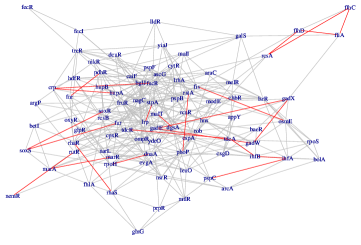
Figure 2. Estimated conditional independence graph in a Gaussian copula model for data on the expression of 87 transcription factors in E. coli.

Example 1.3 involves a number of pre-selected genes and is thus of moderate dimensionality. Modern experiments often yield far higher-dimensional data, presenting a statistical challenge that is behind much of the recent fascination with graphical models.

1.3. Outline of the Review

This review begins with more background on graphical models in Section 2. Sections 3 and 4 discuss structure learning for undirected and directed graphical models. A brief treatment of issues arising from latent variables and heterogeneous data sources is given in Sections 5 and 6. We end with a discussion in Section 7.

While our review conveys some of the main ideas in structure learning, several interesting topics are beyond the scope of our paper. For instance, we do not cover Bayesian inference, even though there is an active Bayesian community whose recent work tackles problems such as heterogeneous data (Peterson et al., 2015; Mitra et al., 2016), latent variables (Silva & Ghahramani, 2009), posterior convergence rates (Banerjee & Ghosal, 2015), robustness (Finegold & Drton, 2014), sampling Markov equivalence classes (He et al., 2013), and context-specific independence (Nyman et al., 2014). We also do not treat dynamic graphical models for multivariate time series, but a discussion of these models can be found in the related paper by Didelez (2016). Another area omitted in this review is active learning; see, e.g., Vats et al. (2014), Statnikov et al. (2015), and Dasarathy et al. (2016).

Finally, the literature on structure learning is vast and our references are necessarily selective. To limit the number of citations, we sometimes only cite a recent paper, trusting that readers will follow the trail of literature to identify earlier work on the topic.

2. Basic Concepts in Graphical Modeling

In this section, we review some essential concepts for undirected and directed graphical models (see, e.g., Lauritzen, 1996; Studený, 2005; Pearl, 2009).

2.1. Undirected Graphical Models

Let $X=(X_{v}:v\in V)$ be a random vector indexed by the vertices of an undirected graph $G=(V,E)$. Then $X$ satisfies the pairwise Markov property with respect to $G$ if

(2.1) $$X_{v}\mathchoice{\mathrel{\hbox to0.0pt{$\displaystyle\perp$\hss}\mkern 3.0mu{\displaystyle\perp}}}{\mathrel{\hbox to0.0pt{$\textstyle\perp$\hss}\mkern 3.0mu{\textstyle\perp}}}{\mathrel{\hbox to0.0pt{$\scriptstyle\perp$\hss}\mkern 3.0mu{\scriptstyle\perp}}}{\mathrel{\hbox to0.0pt{$\scriptscriptstyle\perp$\hss}\mkern 3.0mu{\scriptscriptstyle\perp}}}X_{w}\mid X_{V\setminus\{v,w\}}$$

whenever $\{v,w\}\notin E$. Moreover, $X$ satisfies the local Markov property with respect to $G$ if

(2.2) $$X_{v}\mathchoice{\mathrel{\hbox to0.0pt{$\displaystyle\perp$\hss}\mkern 3.0mu{\displaystyle\perp}}}{\mathrel{\hbox to0.0pt{$\textstyle\perp$\hss}\mkern 3.0mu{\textstyle\perp}}}{\mathrel{\hbox to0.0pt{$\scriptstyle\perp$\hss}\mkern 3.0mu{\scriptstyle\perp}}}{\mathrel{\hbox to0.0pt{$\scriptscriptstyle\perp$\hss}\mkern 3.0mu{\scriptscriptstyle\perp}}}X_{V\setminus(\operatorname{nb}_{G}(v)\cup\{v\})}\mid X_{\operatorname{nb}_{G}(v)}$$

for every $v\in V$, where we recall that $\operatorname{nb}_{G}(v)=\{w\in V:\{w,v\}\in E\}$ is the set of neighbors of $v$. Finally, $X$ satisfies the global Markov property with respect to $G$ if $X_{A}\mathchoice{\mathrel{\hbox to0.0pt{$\displaystyle\perp$\hss}\mkern 3.0mu{\displaystyle\perp}}}{\mathrel{\hbox to0.0pt{$\textstyle\perp$\hss}\mkern 3.0mu{\textstyle\perp}}}{\mathrel{\hbox to0.0pt{$\scriptstyle\perp$\hss}\mkern 3.0mu{\scriptstyle\perp}}}{\mathrel{\hbox to0.0pt{$\scriptscriptstyle\perp$\hss}\mkern 3.0mu{\scriptscriptstyle\perp}}}X_{B}\mid X_{C}$ for all triples of pairwise disjoint subsets $A,B,C\subset V$ such that $C$ separates $A$ and $B$ in $G$, i.e., such that every path between a node in $A$ and a node in $B$ contains a node in $C$.

It is easy to see that the global Markov property implies the pairwise and local properties. It can also be shown that the local Markov property implies the pairwise Markov property. While not true in general, the three Markov properties are equivalent when $X$ satisfies the intersection axiom for conditional independence (Lauritzen, 1996). This equivalence is true in particular when the $X_{v}$ are discrete with positive joint probabilities, or when $X$ has a positive and continuous density with respect to Lebesgue measure.

Example 2.1.

Let $X=(X_{1},\dots,X_{5})$ belong to the graphical model with the undirected graph $G$ in Figure 3. If $X$ satisfies the pairwise Markov property, the missing edges $1-4\notin E$ and $2-4\notin E$ imply $X_{4}\mathchoice{\mathrel{\hbox to0.0pt{$\displaystyle\perp$\hss}\mkern 3.0mu{\displaystyle\perp}}}{\mathrel{\hbox to0.0pt{$\textstyle\perp$\hss}\mkern 3.0mu{\textstyle\perp}}}{\mathrel{\hbox to0.0pt{$\scriptstyle\perp$\hss}\mkern 3.0mu{\scriptstyle\perp}}}{\mathrel{\hbox to0.0pt{$\scriptscriptstyle\perp$\hss}\mkern 3.0mu{\scriptscriptstyle\perp}}}X_{1}\mid(X_{2},X_{3},X_{5})$ and $X_{4}\mathchoice{\mathrel{\hbox to0.0pt{$\displaystyle\perp$\hss}\mkern 3.0mu{\displaystyle\perp}}}{\mathrel{\hbox to0.0pt{$\textstyle\perp$\hss}\mkern 3.0mu{\textstyle\perp}}}{\mathrel{\hbox to0.0pt{$\scriptstyle\perp$\hss}\mkern 3.0mu{\scriptstyle\perp}}}{\mathrel{\hbox to0.0pt{$\scriptscriptstyle\perp$\hss}\mkern 3.0mu{\scriptscriptstyle\perp}}}X_{2}\mid(X_{1},X_{3},X_{5})$. The local Markov property for node $v=4$ implies $X_{4}\mathchoice{\mathrel{\hbox to0.0pt{$\displaystyle\perp$\hss}\mkern 3.0mu{\displaystyle\perp}}}{\mathrel{\hbox to0.0pt{$\textstyle\perp$\hss}\mkern 3.0mu{\textstyle\perp}}}{\mathrel{\hbox to0.0pt{$\scriptstyle\perp$\hss}\mkern 3.0mu{\scriptstyle\perp}}}{\mathrel{\hbox to0.0pt{$\scriptscriptstyle\perp$\hss}\mkern 3.0mu{\scriptscriptstyle\perp}}}(X_{1},X_{2})\mid(X_{3},X_{5})$. The global Markov property explicitly requires many other conditional independencies, such as for example $X_{4}\mathchoice{\mathrel{\hbox to0.0pt{$\displaystyle\perp$\hss}\mkern 3.0mu{\displaystyle\perp}}}{\mathrel{\hbox to0.0pt{$\textstyle\perp$\hss}\mkern 3.0mu{\textstyle\perp}}}{\mathrel{\hbox to0.0pt{$\scriptstyle\perp$\hss}\mkern 3.0mu{\scriptstyle\perp}}}{\mathrel{\hbox to0.0pt{$\scriptscriptstyle\perp$\hss}\mkern 3.0mu{\scriptscriptstyle\perp}}}X_{2}\mid(X_{1},X_{3})$ or $(X_{4},X_{5})\mathchoice{\mathrel{\hbox to0.0pt{$\displaystyle\perp$\hss}\mkern 3.0mu{\displaystyle\perp}}}{\mathrel{\hbox to0.0pt{$\textstyle\perp$\hss}\mkern 3.0mu{\textstyle\perp}}}{\mathrel{\hbox to0.0pt{$\scriptstyle\perp$\hss}\mkern 3.0mu{\scriptstyle\perp}}}{\mathrel{\hbox to0.0pt{$\scriptscriptstyle\perp$\hss}\mkern 3.0mu{\scriptscriptstyle\perp}}}(X_{1},X_{2})\mid X_{3}$.

Figure 3. An undirected graph with five nodes.

The pairwise Markov property for undirected graphical models translates each absent edge into a ‘full’ conditional independence. For this reason, the smallest undirected graph $G$ with respect to which $X$ is pairwise Markov is also known as the conditional independence graph of $X$. Testing all $\binom{|V|}{2}$ pairwise full conditional independencies that might arise in (2.1) yields a method to estimate this graph. Addressing the multiple testing issues in this approach allows for control of false edge discoveries. We will not discuss this in detail but refer the reader to Drton & Perlman (2007), Liu (2013), and Wasserman et al. (2014).

Under the local Markov property, each variable $X_{v}$ can be optimally predicted from its neighbors $X_{\operatorname{nb}(v)}$, which is used in a method known as neighborhood selection (see Section 3). The global Markov property on the other hand is very useful for reasoning about conditional independence.

The famous theorem of Hammersley and Clifford clarifies the construction of distributions that possess the Markov properties. Suppose $X=(X_{v}:v\in V)$ has a density with respect to a product measure $\mu=\otimes_{v\in V}\mu_{v}$ on $\mathbb{R}^{V}$. In applications, each $\mu_{v}$ is usually either Lebesgue or a counting measure, so each $X_{v}$ is (absolutely) continuous or discrete. Let $\mathcal{C}(G)$ be the set of all complete subsets (or cliques) of $G$, i.e., $C\in\mathcal{C}(G)$ if $\{v,w\}\in E$ for all $v,w\in C$. Then the distribution of $X$ is said to factorize with respect to $G$ if it has a density of the form

(2.3) $$f(x)\;=\;\prod_{C\in\mathcal{C}(G)}\phi_{C}(x_{C}),\quad x\in\mathbb{R}^{V},$$

where each potential function $\phi_{C}$ has domain $\mathbb{R}^{C}$, and $x_{C}$ is the subvector $(x_{v}:v\in C)$. The potential functions need not have a probabilistic interpretation as conditional densities.

Theorem 2.1 (Hammersley-Clifford).

Suppose $X=(X_{v}:v\in V)$ has a positive density with respect to a product measure. Then the distribution of $X$ factorizes with respect to $G=(V,E)$ if and only if $X$ satisfies the pairwise Markov property with respect to $G$.

A graphical model may thus be defined by specifying families of potential functions. If the functions are positive, then the pairwise and global Markov properties are equivalent. Moreover, the global Markov property lists every conditional independence that holds in all distributions with factorizing densities. This is known as completeness of the global Markov property. We remark that factorization of nonpositive distributions for categorical variables is treated by Geiger et al. (2006). Matúš (2012) gives a new perspective on factorization as a consequence of log-convexity of a set of distributions.

Example 2.2.

Suppose $X=(X_{1},\dots,X_{5})$ is centered and multivariate normal with positive definite covariance matrix $\Sigma$. Let $K=(\kappa_{vw})=\Sigma^{-1}$. Then $X$ has density

$$f(x)\;=\;\frac{1}{\sqrt{(2\pi)^{5}\det(\Sigma)}}\exp\left(-\frac{1}{2}\sum_{v,w=1}^{5}\kappa_{vw}x_{v}x_{w}\right),\quad x\in\mathbb{R}^{5}.$$

This distribution factorizes with respect to the graph in Figure 3 if and only if $\kappa_{14}=\kappa_{15}=\kappa_{24}=\kappa_{25}=\kappa_{35}=0$. More generally, the Gaussian model associated with an undirected graph $G=(V,E)$ comprises all normal distributions with a positive definite inverse covariance matrix $K=(\kappa_{vw})\in\mathbb{R}^{V\times V}$ such that $\kappa_{vw}=0$ when $v-w\not\in E$.

Let $S$ be the sample covariance matrix for an i.i.d. Gaussian sample of size $n$. The maximum likelihood estimator (MLE) in the Gaussian graphical model maximizes the log-likelihood function

(2.4) $$L(K)\;=\;\log\det(K)-\text{tr}\left(SK\right)$$

subject to $K$ being positive definite with zeros over non-edges of $G$. Strictly speaking, (2.4) is obtained by maximizing over an unknown mean vector, dividing out $n/2$, and omitting an additive constant. If $n>|V|$, then $L$ admits a unique maximizer with probability one, because $S$ is almost surely positive definite. If $|V|\geq n$, then $S$ is singular and $L$ can be unbounded. However, if the graph $G$ is sparse, then the MLE of $K$ may exist uniquely with probability one even if $n$ is much smaller than $|V|$; see, e.g., Sullivant & Gross (2014).

2.2. Directed Graphical Models

Directed acyclic graphs (DAGs) are directed graphs without directed cycles. A random vector $X=(X_{v}:v\in V)$ satisfies the local Markov property with respect to a DAG $G$ if

$$X_{v}\mathchoice{\mathrel{\hbox to0.0pt{$\displaystyle\perp$\hss}\mkern 3.0mu{\displaystyle\perp}}}{\mathrel{\hbox to0.0pt{$\textstyle\perp$\hss}\mkern 3.0mu{\textstyle\perp}}}{\mathrel{\hbox to0.0pt{$\scriptstyle\perp$\hss}\mkern 3.0mu{\scriptstyle\perp}}}{\mathrel{\hbox to0.0pt{$\scriptscriptstyle\perp$\hss}\mkern 3.0mu{\scriptscriptstyle\perp}}}X_{\operatorname{nd}_{G}(v)\setminus\operatorname{pa}_{G}(v)}\,|\,X_{\operatorname{pa}_{G}(v)}$$

for every $v\in V$. Similarly, $X$ satisfies the global Markov property with respect to $G$ if $X_{A}\mathchoice{\mathrel{\hbox to0.0pt{$\displaystyle\perp$\hss}\mkern 3.0mu{\displaystyle\perp}}}{\mathrel{\hbox to0.0pt{$\textstyle\perp$\hss}\mkern 3.0mu{\textstyle\perp}}}{\mathrel{\hbox to0.0pt{$\scriptstyle\perp$\hss}\mkern 3.0mu{\scriptstyle\perp}}}{\mathrel{\hbox to0.0pt{$\scriptscriptstyle\perp$\hss}\mkern 3.0mu{\scriptscriptstyle\perp}}}X_{B}\mid X_{C}$ for all triples of pairwise disjoint subsets $A,B,C\subset V$ such that $C$ d-separates $A$ and $B$ in $G$, which we denote by $A\perp_{G}B\,|\,C$. The notion of d-separation in directed graphs is more subtle than separation in undirected graphs. We refer to Definition 2.1 below.

If $X$ satisfies the global Markov property with respect to $G$, then $G$ is called an independence map of $X$. A DAG $G$ is a perfect map of $X$ if $A\perp_{G}B\,|\,C$ if and only if $X_{A}\mathchoice{\mathrel{\hbox to0.0pt{$\displaystyle\perp$\hss}\mkern 3.0mu{\displaystyle\perp}}}{\mathrel{\hbox to0.0pt{$\textstyle\perp$\hss}\mkern 3.0mu{\textstyle\perp}}}{\mathrel{\hbox to0.0pt{$\scriptstyle\perp$\hss}\mkern 3.0mu{\scriptstyle\perp}}}{\mathrel{\hbox to0.0pt{$\scriptscriptstyle\perp$\hss}\mkern 3.0mu{\scriptscriptstyle\perp}}}X_{B}\,|\,X_{C}$ for all pairwise disjoint sets $A,B,C\subset V$. A perfect map thus requires the global Markov property and its reverse implication, known as faithfulness. The assumption that $G$ is a perfect map is important for the structure learning methods that we discuss in Section 4.

Suppose $X$ has a density with respect to a product measure. Then the distribution of $X$ factorizes according to a DAG $G=(V,E)$ if it has a density of the form

(2.5) $$f(x)=\prod_{v\in V}f(x_{v}\,|\,x_{\operatorname{pa}_{G}(v)}),$$

where the $f(x_{v}\,|\,x_{\operatorname{pa}_{G}(v)})$ are conditional densities with $f(x_{v}\,|\,x_{\emptyset})=f(x_{v})$. The global and local Markov properties are equivalent, and under the assumed existence of a density they are equivalent to the factorization property (Verma & Pearl, 1988). The global Markov property is also complete, i.e., it states all conditional independencies that are implied by the factorization.

A directed graphical model for a DAG $G$ can be specified by conditional densities $f(x_{v}\,|\,x_{\operatorname{pa}_{G}(v)})$, $v\in V$. If these do not share common parameters, the likelihood function of the model factorizes into $|V|$ local likelihood functions, and the MLEs of $f(x_{v}\,|\,x_{\operatorname{pa}_{G}(v)})$, $v\in V$, can be computed separately. For categorical data, this amounts to computing empirical frequencies for conditional probability tables. For multivariate Gaussian data, the conditional means and variances are found via linear regression of each $X_{v}$ on $X_{\operatorname{pa}_{G}(v)}$.

We now define d-separation. In a DAG $G=(V,E)$, nodes $v$ and $w$ are adjacent if $v\to w\in E$ or $w\to v\in E$, and a path is a sequence of distinct nodes in which successive nodes are adjacent. If $\pi=(v_{0},v_{1},\dots,v_{k})$ is a path, then $v_{0}$ and $v_{k}$ are the endpoints of the path. A non-endpoint $v_{i}$ is a collider on $\pi$ if $v_{i-1}\to v_{i}\leftarrow v_{i+1}$ is a subpath of $\pi$. Otherwise, $v_{i}$ is a non-collider on $\pi$. If every edge on $\pi$ is of the form $v_{i-1}\to v_{i}$, then $v_{0}$ is an ancestor of $v_{k}$ and $v_{k}$ is a descendent of $v_{0}$. We write $\operatorname{adj}_{G}(v)$, $\operatorname{an}_{G}(v)$ and $\operatorname{de}_{G}(v)$ for the sets of adjacent nodes, ancestors and descendants of $v$ in $G$, respectively. We use the convention that $v$ is an ancestor and descendant of itself, and apply the notions disjunctively to sets, e.g., $\operatorname{an}_{G}(C)=\cup_{v\in C}\operatorname{an}_{G}(v)$. Finally, we define $\operatorname{nd}_{G}(C)=V\setminus\operatorname{de}_{G}(C)$.

Definition 2.1.

Two nodes $v$ and $w$ in a DAG $G=(V,E)$ are d-connected given $C\subseteq V\setminus\{v,w\}$ if $G$ contains a path $\pi$ with endpoints $v$ and $w$ such that (i) all colliders on $\pi$ are in $\operatorname{an}_{G}(C)$, and (ii) no non-collider on $\pi$ is in $C$. Generalizing to sets, two disjoint subsets $A,B\subset V$ are d-connected given $C\subseteq V\setminus(A\cup B)$ if there are two nodes $v\in A$ and $w\in B$ that are d-connected given $C$. If this is not the case, then $C$ d-separates $A$ and $B$.

((a)) A DAG $G$.

((b)) The CPDAG of $G$.

((c)) The moral graph of $G$.

Figure 4. An example to illustrate Markov properties, the CPDAG, and the moral graph.

Example 2.3.

Let $X=(X_{1},\dots,X_{5})$ belong to the graphical model with the DAG $G$ in Figure 4(a). We see that node 2 is a collider on the path $1\to 2\leftarrow 3\to 4$, while it is a non-collider on $1\to 2\to 5$. For node $4$, the local Markov property requires $X_{4}\mathchoice{\mathrel{\hbox to0.0pt{$\displaystyle\perp$\hss}\mkern 3.0mu{\displaystyle\perp}}}{\mathrel{\hbox to0.0pt{$\textstyle\perp$\hss}\mkern 3.0mu{\textstyle\perp}}}{\mathrel{\hbox to0.0pt{$\scriptstyle\perp$\hss}\mkern 3.0mu{\scriptstyle\perp}}}{\mathrel{\hbox to0.0pt{$\scriptscriptstyle\perp$\hss}\mkern 3.0mu{\scriptscriptstyle\perp}}}(X_{1},X_{2},X_{5})\,|\,X_{3}$. Since $1$ and $4$ are d-connected given $C=\{2\}$, $C=\{5\}$ and $C=\{2,5\}$, but d-separated given any other subset of $\{2,3,5\}$, the global Markov property requires $X_{1}\mathchoice{\mathrel{\hbox to0.0pt{$\displaystyle\perp$\hss}\mkern 3.0mu{\displaystyle\perp}}}{\mathrel{\hbox to0.0pt{$\textstyle\perp$\hss}\mkern 3.0mu{\textstyle\perp}}}{\mathrel{\hbox to0.0pt{$\scriptstyle\perp$\hss}\mkern 3.0mu{\scriptstyle\perp}}}{\mathrel{\hbox to0.0pt{$\scriptscriptstyle\perp$\hss}\mkern 3.0mu{\scriptscriptstyle\perp}}}X_{4}\,|\,X_{C^{\prime}}$ for any such other subset $C^{\prime}$ of $\{2,3,5\}$. We observe that, in contrast to separation in undirected graphs, d-separation in a DAG is not monotonic in the sense that $A\perp_{G}B\,|\,C$ does not imply that $A\perp_{G}B\,|\,C^{\prime}$ for sets $C^{\prime}\supsetneq C$. Note also that there does not exist an undirected graph that encodes the same conditional independencies as the DAG in Figure 4(a). Finally, the factorization for $G$ takes the form $f(x)=f(x_{1})f(x_{2}|x_{1},x_{3})f(x_{3})f(x_{4}|x_{3})f(x_{5}|x_{2})$.

Two DAGs $G$ and $G^{\prime}$ are Markov equivalent if $A\perp_{G}B\,|\,C$ is equivalent to $A\perp_{G^{\prime}}B\,|\,C$. Markov equivalent DAGs are characterized by having the same skeleton and the same v-structures (Frydenberg, 1990; Verma & Pearl, 1991). A v-structure is a triple of nodes $u\to v\leftarrow w$ with $u$ and $w$ not adjacent. Each Markov equivalence class can be represented by a completed partially directed acyclic graph (CPDAG) that may have directed and undirected edges (e.g., Andersson et al., 1997; Roverato, 2005). A CPDAG has edge $v\to w$ if and only if the edge $v\to w$ is common to all DAGs in its equivalence class. If the class contains a DAG with $v\to w$ and a DAG with $v\leftarrow w$, then the CPDAG has the undirected edge $v-w$. The DAG $G$ in Figure 4(a) is Markov equivalent to exactly one other DAG, obtained by replacing the edge $3\to 4$ by $3\leftarrow 4$. The CPDAG of $G$ is shown in Figure 4(b).

The skeleton of a (partially) directed graph is the undirected graph obtained by replacing all edges by undirected edges. The moral graph $G^{m}$ of a DAG $G$ is constructed by first shielding all v-structures and then taking the skeleton of the resulting graph. Shielding a v-structure $u\to v\leftarrow w$ means adding an edge between nodes $u$ and $w$. Figure 4(c) shows the moral graph of the DAG in Figure 4(a). It is easy to see that if $X$ satisfies the factorization property for directed graphs with respect to $G$, then $X$ satisfies the factorization property for undirected graphs with respect to the moral graph $G^{m}$. Hence, if $G$ is a perfect map of $X$, then $G^{m}$ is the conditional independence graph of $X$. This implies that the skeleton of a DAG (or CPDAG) is a subgraph of its corresponding conditional independence graph.

The graphical model associated with a DAG $G=(V,E)$ can also be thought of as a structural equation model (Bollen, 1989). Indeed, if $\epsilon=(\epsilon_{v}:v\in V)$ is a vector of independent random noise variables and $g_{v}$ are measurable functions, then the random vector $X=(X_{v}:v\in V)$ given by

(2.6) $$X_{v}\;=\;g_{v}(X_{\operatorname{pa}_{G}(v)},\epsilon_{v}),\quad v\in V,$$

is Markov with respect to $G$. Conversely, if $X$ is Markov with respect to $G$, then there are independent variables $\epsilon_{v}$ and functions $g_{v}$ such that (2.6) holds.

Example 2.4.

If all functions $g_{v}$ are linear and the $\epsilon_{v}$ are normal random variables, then we may assume that (2.6) takes the form $X=BX+\epsilon$, where the matrix $B=(\beta_{vw})\in\mathbb{R}^{V\times V}$ has $\beta_{vw}=0$ if $w\not\in\operatorname{pa}_{G}(v)$. The solution $X=(I-B)^{-1}\epsilon$ follows a multivariate normal distribution with covariance matrix $\operatorname{Cov}(X)=(I-B)^{-1}\operatorname{Cov}(\epsilon)(I-B)^{-T}$. Here, $I-B$ is invertible since $\det(I-B)=1$ by acyclicity of $G$.

Structural equation models, and thus also directed graphical models, admit a natural causal interpretation. To this end, one views the equations in (2.6) as specifying an assignment mechanism, which is clarified by writing

(2.7) $$X_{v}\leftarrow g_{v}(X_{\operatorname{pa}_{G}(v)},\epsilon_{v}),\quad v\in V.$$

The variables in $X_{\operatorname{pa}_{G}(v)}$ are then treated as direct causes of $X_{v}$, meaning that changes in $X_{\operatorname{pa}_{G}(v)}$ may lead to changes in $X_{v}$, but not the other way around. This interpretation allows statements about the distribution of $X$ under experimental interventions. In particular, interventions to the system can be modeled by changing the structural equations for precisely those variables that are affected by the intervention (Pearl, 2009).

Example 2.5.

The structural equation model for the DAG in Figure 4(a) postulates that

$$X_{1} \leftarrow g_{1}(\epsilon_{1}), X_{3} \leftarrow g_{3}(\epsilon_{3}), X_{2} \leftarrow g_{2}(X_{1},X_{3},\epsilon_{2}), X_{4} \leftarrow g_{4}(X_{3},\epsilon_{4}), X_{5} \leftarrow g_{5}(X_{2},\epsilon_{5}).$$

We now consider an intervention on $X_{2}$, where $X_{2}$ is generated as an independent draw from the distribution of $\epsilon_{2}$. Denoting the post-intervention variables by $\tilde{X}=(\tilde{X}_{v}:v\in V)$, the distribution of $\tilde{X}$ is induced by the equation system

$$\tilde{X}_{1} =g_{1}(\epsilon_{1}), \tilde{X}_{3} =g_{3}(\epsilon_{3}), \tilde{X}_{2} =\epsilon_{2}, \tilde{X}_{4} =g_{4}(\tilde{X}_{3},\epsilon_{4}), \tilde{X}_{5} =g_{5}(\tilde{X}_{2},\epsilon_{5}).$$

The post-intervention DAG $\tilde{G}$ is obtained from $G$ by removing the edges $1\to 2$ and $3\to 2$.

Thus, the causal interpretation of a DAG allows predictions in changed environments, and hence the estimation of causal effects. These ideas can be combined with the structure learning methods that we discuss in Section 4 to estimate (bounds on) causal effects from observational data (Maathuis et al., 2009, 2010; Perković et al., 2015; Nandy et al., 2016b).

3. Learning Undirected Graphical Models

Our treatment of learning undirected graphical models begins with the special case of trees. We then move on to generally applicable greedy search and $\ell_{1}$ penalization methods as well as techniques that avoid traditional assumptions of Gaussianity for continuous observations.

3.1. Chow-Liu Trees and Forests

A tree $G=(V,E)$ is an undirected graph with a unique path between any two nodes, and thus $|E|=|V|-1$. Chow & Liu (1968) showed that one can efficiently find a tree-structured distribution that optimally approximates a given distribution. In the present context, we may view their algorithm as outputting a maximum likelihood (ML) estimate of a conditional independence tree.

Due to convenient factorizations, computation in tree-based graphical models is particularly tractable (Wainwright & Jordan, 2008). Indeed, if the distribution of a random vector $X=(X_{v}:v\in V)$ factorizes with respect to a tree, then the joint density factorizes as

(3.1) $$f(x)\;=\;\prod_{v-w\in E}\frac{f_{vw}(x_{v},x_{w})}{f_{v}(x_{v})f_{w}(x_{w})}\prod_{v\in V}f_{v}(x_{v}).$$

Here, $f_{v}$ and $f_{vw}$ are the marginal densities of $X_{v}$ and $(X_{v},X_{w})$, respectively. Formula (3.1) is a special case of a more general result exemplified in (3.2). It coincides with (2.5) when we create a directed tree by letting edges point away from one arbitrarily selected node.

Suppose for a moment that all variables are categorical, with $X_{v}$ taking values in a finite set $\mathcal{X}_{v}$. For a joint state $x\in\mathcal{X}:=\prod_{v\in V}\mathcal{X}_{v}$, let $N(x)$ be the number of times $x$ appears in an i.i.d. sample of size $n$ from the distribution of $X$. Writing $\hat{f}_{G}(x)$ for the ML estimate of the joint probability $f(x)$ in the graphical model given by tree $G$, we aim to find the tree $G$ with largest maximum log-likelihood $\hat{L}(G)=\sum_{x\in\mathcal{X}}N(x)\log\hat{f}_{G}(x).$

Let $\hat{f}_{vw}(x_{v},x_{w})$ and $\hat{f}_{v}(x_{v})$ be the relative frequencies of seeing the pair $(X_{v},X_{w})$ in state $(x_{v},x_{w})$ and variable $X_{v}$ in state $x_{v}$, respectively. The MLE $\hat{f}_{G}(x)$ is obtained by plugging the $\hat{f}_{vw}$ and $\hat{f}_{v}$ into (3.1). It follows that

$$\frac{1}{n}\hat{L}(G)\;=\;\sum_{v-w\in E}I\big{(}\hat{f}_{vw}\big{)}+\text{const.},$$

where $I(\hat{f}_{vw})$ is the empirical mutual information of $X_{v}$ and $X_{w}$, so

$$I\big{(}\hat{f}_{vw}\big{)}\;=\;\sum_{x_{v}\in\mathcal{X}_{v}}\sum_{x_{w}\in\mathcal{X}_{w}}\hat{f}_{vw}(x_{v},x_{w})\log\frac{\hat{f}_{vw}(x_{v},x_{w})}{\hat{f}_{v}(x_{v})\hat{f}_{w}(x_{w})}.$$

Since mutual information is non-negative, the ML tree is a maximum spanning tree for the complete graph with edge weights $I(\hat{f}_{vw})$. The maximum spanning tree can be computed efficiently using, e.g., Kruskal’s algorithm, which adds edges $\{v,w\}$ in the order of decreasing mutual information $I(\hat{f}_{vw})$ but skips edges that create a cycle. The ML tree is found after addition of $|V|-1$ edges. If Kruskal’s algorithm is stopped early, adding only $k$ edges, then the output is a forest with maximum likelihood among all forests with $k$ edges. A forest is an undirected graph that is a union of disconnected trees.

The Chow-Liu method is not limited to categorical data. Indeed, we may formulate statistical models for the bivariate marginal distributions $f_{vw}$, compute their ML estimates $\hat{f}_{vw}$ and find a maximum weight spanning tree from their mutual informations $I(\hat{f}_{vw})$. In particular, when the marginals are taken to be bivariate normal then the joint density $f$ is multivariate normal and $I(\hat{f}_{vw})=-\frac{1}{2}\log(1-r_{vw}^{2})$, where $r_{vw}$ is the empirical correlation between $X_{v}$ and $X_{w}$. In this case, the absolute correlations $|r_{vw}|$ can also be used as weights.

While it is an older idea, there has been renewed interest in Chow and Liu’s approach. Tan et al. (2010, 2011) study which trees/forests are most difficult to recover. Liu et al. (2011) use kernel density estimates in a nonparametric approach. Edwards et al. (2010) discuss mixed categorical and continuous data and incorporate information criteria into the algorithm. The output is then a forest because the penalties for model complexity may yield negative edge weights. Treating models with latent variables, Friedman et al. (2002) suggested a structural EM algorithm whose M-step optimizes over both parameters and tree structure. The Chow-Liu algorithm was also used in methods for learning latent locally tree-like graphs by Anandkumar & Valluvan (2013).

3.2. Greedy Search

Beyond the realm of trees, finding a graph that maximizes a (penalized) likelihood or information criterion is hard in a complexity-theoretic sense (Karger & Srebro, 2001). Nevertheless, good estimates can be obtained from heuristic techniques, such as greedy or stepwise forward/backward search. Good implementations, e.g., as discussed by Højsgaard et al. (2012), evaluate the benefit of an edge addition or removal via local computations based on clique-sum decompositions (Lauritzen, 1996, Chap. 3).

Example 3.1.

The graph $G$ in Figure 5(a) is a clique-sum of three smaller graphs, the so-called prime components shown in Figure 5(b). If a distribution factorizes with respect to $G$, then its density $f$ satisfies

(3.2) $$f(x)\;=\;\frac{f_{1234}(x_{1},x_{2},x_{3},x_{4})f_{345}(x_{3},x_{4},x_{5})f_{567}(x_{5},x_{6},x_{7})}{f_{34}(x_{3},x_{4})f_{5}(x_{5})}.$$

The marginal densities in the numerator correspond to the prime components, and those in the denominator correspond to the separating sets, i.e., the cliques along which the prime components are summed. Suppose now that we wish to compute the likelihood ratio statistic comparing the given graph to the graph with edge $3-5$ removed, in a setting of categorical data under multinomial sampling. The edge belongs to the clique $\{3,4,5\}$, Proposition 4.32 in Lauritzen (1996) implies that the likelihood ratio statistic can be obtained by computing with the data on $(X_{3},X_{4},X_{5})$ alone. Specifically, one computes the likelihood ratio of the graph $3-4-5$ with respect to the full triangle graph on $\{3,4,5\}$. Analogous results exist for the Gaussian case and, with additional subtleties, for mixed discrete and conditionally Gaussian observations (Lauritzen, 1996, Chap. 5 and 6).

Computation of likelihood ratios is particularly convenient for decomposable graphs, i.e., graphs in which all prime components are complete. For example, trees are decomposable because their prime components are the individual edges, and the graph in Figure 5(a) is non-decomposable. For a decomposable graph, Gaussian models as well as models for categorical variables admit closed form MLEs (Lauritzen, 1996, Sections 4.4, 5.3). These are obtained by estimating marginal distributions (via sample means and covariances for Gaussian data, or via empirical frequencies for categorical data) and substituting these estimates in a factorization such as (3.2). In contrast, computing MLEs for non-decomposable graphs involves solving higher degree polynomial equation systems (Drton et al., 2009, Chap. 2.1).

((a)) An undirected graph.

((b)) Clique-sum of its prime components.

Figure 5. A clique-sum decomposition.

More recently, greedy search has been applied in a framework of neighborhood selection, in which a graph $G$ is selected by determining the neighborhood $\operatorname{nb}_{G}(v)$ of each node $v$. As discussed in Section 3.4, finding $\operatorname{nb}_{G}(v)$ often corresponds to variable selection in a regression problem. This avoids the need for iterative computation of MLEs when dealing with non-decomposable graphs, and a connection can be made to results on forward selection methods for variable selection in high-dimensional regression. Jalali et al. (2011) and Ray et al. (2015) leverage this connection and provide theoretical guarantees for greedy search in high-dimensional problems. The related method of Bresler (2015) greedily selects supersets of the neighborhoods that are subsequently pruned. These methods are competitive to the $\ell_{1}$-regularization techniques that we discuss next.

3.3. Gaussian Models and $\ell_{1}$-Penalization

Gaussian models provide the starting point for most graphical modeling of continuous observations. As noted in Example 2.2, a Gaussian conditional independence graph can be estimated by determining the zero entries of the inverse covariance matrix $K\in\mathbb{R}^{V\times V}$.

Let $S=(s_{vw})$ be the sample covariance matrix for a sample of $n$ observations, with $s_{vv}>0$ for all $v\in V$ to avoid trivialities. Yuan & Lin (2007) and Banerjee et al. (2008) proposed the graphical lasso (glasso) estimator

(3.3) $$\hat{K}^{\rm gl}\;=\;\arg\min_{K}\;\Big{\{}-\log\det(K)+\text{tr}\left(SK\right)+\lambda\|K\|_{1}\Big{\}},$$

where the minimization is over positive definite matrices $K=(\kappa_{vw})\in\mathbb{R}^{V\times V}$ and $\lambda\geq 0$ is a tuning parameter. The objective adds to the log-likelihood function from (2.4) a multiple of the (vector) $\ell_{1}$-norm, i.e., $\|K\|_{1}=\sum_{v,w\in V}|\kappa_{vw}|$. Some authors omit the positive diagonal entries $\kappa_{vv}$ when forming the norm. In either case, such a regularization term induces sparsity in $\hat{K}^{\rm gl}$, just as it does in lasso regression. The conditional independence graph is then estimated by the graph $\hat{G}^{\rm gl}$ that has edge $v-w$ if and only if $\hat{\kappa}^{\rm gl}_{vw}\not=0$. For $\lambda>0$, the minimum in (3.3) is achieved uniquely because the objective is strictly concave and coercive irrespective of whether $S$ has full rank. This is important in high-dimensional settings.

The coordinate-descent algorithm of Friedman et al. (2008) is a popular method for computation of $\hat{K}^{\rm gl}$; see Mazumder & Hastie (2012b) for a discussion of its properties. Recent implementations exploit that simply thresholding the sample covariance matrix $S$ yields the connected components of $\hat{G}^{\rm gl}$ (Witten et al., 2011; Mazumder & Hastie, 2012a). Alternative approaches for computation of $\hat{K}^{\rm gl}$ are discussed in Hsieh et al. (2013). The estimation error of $\hat{K}^{\rm gl}$ and the consistency of $\hat{G}^{\rm gl}$ in high-dimensional problems are studied by Ravikumar et al. (2011).

There are several related methods to estimate a sparse covariance matrix. For example, Cai et al. (2011) minimize $\|K\|_{1}$ subject to a constraint on $\|SK-I\|_{\infty}$. Here, $I$ is the identity and $\|A\|_{\infty}$ is the maximum absolute entry of $A$. Minimax optimality properties can be proven for an adaptive version of the estimator (Cai et al., 2016).

A conditional independence graph is sometimes expected to have particular structure, such as ‘hub’ nodes with many neighbors. This motivated Defazio & Caetano (2012) to consider regularization with a sorted $\ell_{1}$ norm. For tuning parameters $\lambda_{1}\geq\dots\geq\lambda_{p}\geq 0$, the sorted $\ell_{1}$ norm of $\beta\in\mathbb{R}^{p}$ is $\sum_{j=1}^{p}\lambda_{j}|\beta_{(j)}|$, where $\beta_{(1)},\dots,\beta_{(p)}$ are the entries of $\beta$ listed in descending order of absolute values, so $|\beta_{(1)}|\geq|\beta_{(2)}|\geq\dots\geq|\beta_{(p)}|$. Defazio & Caetano (2012) estimate the inverse covariance $K=(\kappa_{vw})$ by the optimal solution of

(3.4) $$\min_{K}\;\Big{\{}-\log\det(K)+\text{tr}\left(SK\right)+\sum_{v\in V}\sum_{j=1}^{|V|}\lambda_{j}|\kappa_{v,(j)}|\Big{\}}.$$

Intuitively, the sorted $\ell_{1}$ norm allows one to more easily detect a signal $\kappa_{vw}$ if it concerns a variable $X_{v}$ with other stronger signals $\kappa_{vu}$. Of course, the work just described is not the only one addressing hubs (see e.g., Tan et al., 2014).

3.4. Neighborhood Selection

We may estimate a conditional independence graph $G=(V,E)$ by estimating all of its neighborhoods $\operatorname{nb}_{G}(v)$. According to the local Markov property, $X_{v}$ depends on the other variables only through its neighbors $X_{w}$, $w\in\operatorname{nb}_{G}(v)$. Hence, we may proceed by estimating the conditional distribution of $X_{v}$ given $X_{V\setminus\{v\}}$, and determine $\operatorname{nb}_{G}(v)$ as the index set of the variables $X_{w}$ on which the estimated conditional distribution depends. The ideas behind this neighborhood selection have a longer tradition (Besag, 1975). However, its wide-spread use in graphical modeling emerged more recently when Meinshausen & Bühlmann (2006) tackled high-dimensional problems through a connection to lasso regression.

Example 3.2.

Let $X=(X_{v}:v\in V)$ be multivariate normal with inverse covariance matrix $K=(\kappa_{vw})$. Then the conditional distribution of $X_{v}$ given all remaining variables is normal with variance $1/\kappa_{vv}$ and expectation

$$\operatorname{\mathbb{E}}\left[X_{v}\,|\,X_{w},\,w\not=v\right]\;=\;\sum_{w\in V\setminus\{v\}}\left(-\frac{\kappa_{vw}}{\kappa_{vv}}\right)X_{w}\;=\;\sum_{w\in\operatorname{nb}_{G}(v)}\left(-\frac{\kappa_{vw}}{\kappa_{vv}}\right)X_{w}.$$

We may estimate $\operatorname{nb}_{G}(v)$ as the set of active covariates in a linear regression of $X_{v}$ on all other variables $X_{w}$, $w\not=v$. Any technique for variable selection could be applied.

Example 3.3.

In a symmetric Ising model with (real-valued) interaction parameters $\theta_{vw}$, all random variables $X_{v}$ take values in $\{-1,1\}$ and joint probabilities have the form

(3.5) $$\Pr(X_{v}=x_{v},\,v\in V)\;\propto\;\exp\Bigg{\{}\sum_{\{v,w\}\in E}\theta_{vw}x_{v}x_{w}\Bigg{\}}.$$

By the Hammersley-Clifford theorem, the conditional independence graph $G=(V,E)$ of such a distribution has edge $v-w\in E$ if and only if $\theta_{vw}\not=0$. Since

$$\log\left(\frac{\Pr(X_{v}=1\,|\,X_{w}=x_{w},\,w\not=v)}{1-\Pr(X_{v}=1\,|\,X_{w}=x_{w},\,w\not=v)}\right)\;=\;\sum_{w\in\operatorname{nb}_{G}(v)}\left(2\theta_{vw}\right)x_{w},$$

the neighborhood $\operatorname{nb}_{G}(v)$ can be estimated as the set of active covariates in a logistic regression of $X_{v}$ on all other variables $X_{w}$, $w\not=v$. We note that the normalizing constant in (3.5) is a sum over $2^{|V|}$ joint states and thus intractable unless $|V|$ is small.

Estimating each neighborhood in isolation may lead to inconsistencies that are commonly resolved post-hoc. Let $\widehat{\operatorname{nb}}(v)$, $v\in V$, be the estimated neighborhoods. If $w\in\widehat{\operatorname{nb}}(v)$ but $v\not\in\widehat{\operatorname{nb}}(w)$, then the so-called ‘and’-rule excludes the edge $v-w$ from the estimated conditional independence graph, while the ‘or’-rule includes such edges.

The use of $\ell_{1}$-regularization for neighborhood selection in Gaussian and Ising models (Examples 3.2 and 3.3) is studied by Meinshausen & Bühlmann (2006) and Ravikumar et al. (2010), respectively. Yang et al. (2015a) treat other exponential family models, and Chen et al. (2015) propose refinements of the ‘and’/‘or’-rules that take into account the distributional type of the nodes. Voorman et al. (2014) apply techniques for sparse additive models, in which a conditional expectation of the form $\operatorname{\mathbb{E}}\left[X_{v}\,|\,X_{w},\,w\not=v\right]\;=\;\sum_{w\not=v}f_{vw}(X_{w})$ is estimated using basis expansions and a group lasso penalty that allows for zero functions as estimates of some of the univariate functions $f_{vw}$.

Neighborhood selection is related to the concept of pseudo-likelihood, which is based on the full conditional densities of a joint density $f$. The log-pseudo-likelihood function is

(3.6) $$L_{\rm pseudo}(f)\;=\;\sum_{v\in V}\log f_{v|V\setminus\{v\}}\left(x_{v}\,|\,x_{w},\,w\not=v\right).$$

Non-Gaussian distributions specified via the Hammersley-Clifford theorem typically have intractable normalizing constants; recall Example 3.3. In contrast, the full conditionals in the pseudo-likelihood can often be normalized. Indeed, the conditional probabilities for discrete $X_{v}$ can be normalized by summing over the state space of $X_{v}$ alone as opposed to over all joint states. Similarly, it may be feasible to find the normalizing constant of the full conditional density for a continuous random variable by univariate integration.

While neighborhood selection treats the different conditional densities $f_{v|V\setminus\{v\}}$ as unrelated, the conditionals share parameters. For instance, the interaction parameter $\theta_{vw}$ in the Ising model from (3.5) appears in the conditionals for $X_{v}$ and for $X_{w}$. As an alternative that avoids inconsistencies among estimated neighborhoods, we may maximize an $\ell_{1}$ penalized version of $L_{\rm pseudo}$ from (3.6) with respect to a symmetric interaction matrix. Höfling & Tibshirani (2009) explore this pseudo-likelihood method for Ising models but find rather little difference with neighborhood selection. Khare et al. (2015) give an overview of Gaussian pseudo-likelihood methods that retain the symmetry of the inverse covariance matrix and address issues in the specification of a convex optimization objective.

A full likelihood may be expected to yield more efficient estimators than neighborhood selection or pseudo-likelihood. However, under $\ell_{1}$ regularization, the situation is subtle as different irrepresentability conditions are needed to ensure consistency. Indeed, there are Gaussian examples in which neighborhood selection is consistent whenever the glasso is consistent, but in which the converse is false (Meinshausen, 2008; Ravikumar et al., 2011).

3.5. Score Matching

The Hammersley-Clifford theorem allows the specification of graphical models as interaction models in the form of an exponential family. However, the normalizing constants in such models are tractable only in special cases. The score matching approach of Hyvärinen (2005, 2007) is well suited to address this challenge. We describe the basic version that applies to continuous observations supported on all of $\mathbb{R}^{V}$.

Let $X=(X_{v}:v\in V)$ be absolutely continuous with differentiable density $f_{0}$ and support $\mathbb{R}^{V}$. Let $f$ be another density that is twice differentiable and has support $\mathbb{R}^{V}$. Writing $\nabla_{x}$ for the gradient with respect to $x$, define the Fisher information distance

(3.7) $$J(f)\;=\;\int_{\mathbb{R}^{V}}f_{0}(x)\;\left\|\nabla_{x}\log f(x)-\nabla_{x}\log f_{0}(x)\right\|_{2}^{2}\>dx.$$

While it is natural to minimize an estimate of $J(\cdot)$, this approach is complicated by the way the unknown true density $f_{0}$ appears in (3.7). Hyvärinen (2005) circumvents this problem using integration by parts (Stein’s identity), which yields under mild conditions that

(3.8) $$J(f)\;=\;\int_{\mathbb{R}^{V}}f_{0}(x)\left[\Delta_{x}\log f(x)+\frac{1}{2}\|\nabla_{x}\log f(x)\|_{2}^{2}\right]\>dx\;+\;\mbox{const.},$$

where $\Delta_{x}f(x)=\sum_{v}\partial^{2}f(x)/\partial x_{v}^{2}$ is the Laplace operator. Writing $S(x,f)=\Delta_{x}\log f(x)+\frac{1}{2}\|\nabla_{x}\log f(x)\|_{2}^{2}$, a score matching estimator minimizes the empirical loss

$$\hat{J}(f)=\frac{1}{n}\sum_{i=1}^{n}S(x^{(i)},f)$$

for $f$ ranging over a model of interest. Importantly, if $f$ is only known up to a normalizing constant, then this constant cancels in the logarithmic derivatives in $S(x,f)$. Moreover, in an exponential family with log-densities $\log f(x|\theta)=\theta^{T}t(x)-\psi(\theta)+b(x)$ for sufficient statistics $t(x)$, the loss $\hat{J}$ is a convex quadratic function of the natural parameter $\theta$.

Example 3.4.

Consider the family of centered multivariate normal distributions, parameterized by their inverse covariance matrices $K$. Then,

(3.9) $$\hat{J}(K)\;=\;\frac{1}{2}\text{trace}(K^{2}S)-\text{trace}(K)\;=\;\sum_{v\in V}\frac{1}{2}\kappa_{v}^{T}S\kappa_{v}-\kappa_{v}^{T}e_{v},$$

where $S$ is the sample covariance matrix of $X$, $\kappa_{v}$ is the $v$-th column of $K$ and $e_{v}$ is the $v$-th canonical basis vector of $\mathbb{R}^{V}$. If $S$ is invertible then the score matching estimator equals the MLE $\hat{K}=S^{-1}$. However, for submodels that constrain $K$ to lie in a linear subspace, the two estimators generally differ. The score matching estimator need not be asymptotically efficient, as Forbes & Lauritzen (2015) show in the context of symmetry constraints in graphical models.

Closed form score matching estimators are available for any pairwise interaction model

(3.10) $$\log f(x|\theta)\;=\;\sum_{a=1}^{A}\sum_{v\not=w}\theta^{(a)}_{vw}\,t^{(a)}_{vw}(x_{v},x_{w})\>+\>\sum_{l=1}^{L}\sum_{v}\theta^{(l)}_{v}t^{(l)}_{v}(x_{v})\,-\,\psi(\theta)\,+\,b(x),\quad x\in\mathbb{R}^{V},$$

for which $X_{v}\mathchoice{\mathrel{\hbox to0.0pt{$\displaystyle\perp$\hss}\mkern 3.0mu{\displaystyle\perp}}}{\mathrel{\hbox to0.0pt{$\textstyle\perp$\hss}\mkern 3.0mu{\textstyle\perp}}}{\mathrel{\hbox to0.0pt{$\scriptstyle\perp$\hss}\mkern 3.0mu{\scriptstyle\perp}}}{\mathrel{\hbox to0.0pt{$\scriptscriptstyle\perp$\hss}\mkern 3.0mu{\scriptscriptstyle\perp}}}X_{w}\mid X_{V\setminus\{v,w\}}$ if and only if $\theta^{(a)}_{vw}=0$ for all $a=1,\dots,A$. Sparse estimates of the interaction matrices $(\theta^{(a)}_{vw})$ can be obtained by adding an $\ell_{1}$ or group lasso penalty to the loss $\hat{J}$. The resulting estimators of conditional independence graphs are studied by Lin et al. (2016) who also treat nonnegative observations, by Janofsky (2015) who proposes a nonparametric exponential series approach, and by Sun et al. (2015) who consider infinite-dimensional exponential families. For Gaussian models, $\ell_{1}$-regularized score matching is a simple but state-of-the-art method. It coincides with the method of Liu & Luo (2015).

3.6. Semiparametric and Robust Methods

Traditionally, methods for continuous observations rely heavily on Gaussian models. A problem of obvious interest is to provide methods for non-Gaussian observations. We already mentioned a number of such methods and comment here on two other lines of work.

From a perspective of robustness, several authors explored the use of elliptical distributions (Vogel & Fried, 2011; Vogel & Tyler, 2014; Bilodeau, 2014). Finegold & Drton (2011) consider the special case of $t$-distribution models in which a Gaussian random vector is observed under scaling with a single random divisor. They also propose non-elliptical ‘alternative’ $t$-distributions, resulting from dividing the different components of a latent Gaussian vector by independent scalars. Different divisors are useful for high-dimensional data with outliers in many observations, but where each observation only has a small number of corrupted entries.

In a different vein, Liu et al. (2009) propose semiparametric methods based on Gaussian copula models. Here, the observation $X=(X_{v}:v\in V)$ satisfies $X_{v}=h_{v}(Z_{v})$ for a Gaussian random vector $Z=(Z_{v}:v\in V)$ and strictly increasing functions $h_{v}:\mathbb{R}\to\mathbb{R}$. Since the $h_{v}$ are deterministic and one-to-one, $X$ has the same Markov properties as $Z$. Liu et al. (2012a) and Xue & Zou (2012) observe that efficient estimation in the copula models can be based on Kendall’s $\tau$ and Spearman’s $\rho$. Indeed, for strictly increasing $h_{v}$, the observation $X$ and the latent vector $Z$ have the same rank correlations. One may thus apply Gaussian methods after estimating the latent Gaussian correlation matrix by suitably transformed pairwise estimates of $\tau$ or $\rho$. In the data analysis in Example 1.3, we applied this idea in conjunction with Gaussian neighborhood selection from Section 3.4.

It is noteworthy that Kendall’s $\tau$ also provides a simple way to fit copula models based on elliptical distributions (Liu et al., 2012b). Extensions to mixed discrete and continuous data are treated by Fan et al. (2016). Avoiding the assumption of a Gaussian copula, Yang et al. (2014) use coarser data summaries than ranks to handle settings in which the full conditionals are generalized linear models with unknown base measure.

3.7. Tuning Parameter Selection

Many of the aforementioned methods depend on a tuning parameter. Varying this parameter typically yields a useful ranking of edges. However, it may also be desirable to select a single tuning parameter, for example by optimizing information criteria such as the Bayesian information criterion (BIC). However, in problems with a large number of variables $|V|$, the BIC tends to yield overly dense graphs. Foygel & Drton (2010), Gao et al. (2012) and Barber & Drton (2015) address this issue by adapting ideas from sparse high-dimensional regression. Via a multiplicity-correcting prior, the BIC penalty is made dependent on $\log|V|$.

Another useful approach is stability selection (Meinshausen & Bühlmann, 2010; Shah & Samworth, 2013). This method records how often each edge is selected across random subsamples and different tuning parameters, and selects those edges for which there exists a tuning parameter so that the subsample selection frequency exceeds a specified threshold. The method aims at avoiding false positives. A resampling technique that seeks to avoid false negatives was proposed by Liu et al. (2010). This method chooses the least amount of penalization for which graph estimates are suitably stable across subsamples.

Finally, we note that there are methods that aim to reduce or eliminate dependence on tuning parameters; see Lederer & Müller (2014) and references therein.

4. Learning Directed Graphical Models

We now consider learning the structure of a directed graphical model. Textbooks on this problem include Spirtes et al. (2000), Neapolitan (2004), and Koller & Friedman (2009). Throughout, we assume that the DAG $G=(V,E)$ is a perfect map of $X=(X_{v}:v\in V)$, and that we observe $n$ i.i.d. copies of $X$. The observed data are denoted by $\mathbf{x}$.

In general, $G$ is not identifiable from the distribution of $X$, but we can identify its Markov equivalence class, or equivalently, its CPDAG. Thus, many structure learning methods aim to learn the CPDAG. We treat exact score-based search in problems of moderate dimensionality and review more broadly applicable methods based on greedy search or conditional independence tests, as well as hybrids of these two approaches. Finally, we discuss methods that impose additional assumptions that allow identification of the DAG.

4.1. Exact Score-Based Search

Score-based approaches learn a DAG by determining the graph $G$ that optimizes a specified score $Q(G,\mathbf{x})$. Typically $Q$ is a penalized likelihood score, for example the BIC. Such scores are often decomposable, meaning that $Q(G,\mathbf{x})=\sum_{v\in V}q(v\,|\,\operatorname{pa}_{G}(v),\mathbf{x})$, where the summands are local scores of each node $v$ given its parents. Scores such as the BIC are also score-equivalent, meaning that $Q(G,\mathbf{x})=Q(G^{\prime},\mathbf{x})$ if $G$ and $G^{\prime}$ are Markov equivalent.

Finding an optimal DAG, or possibly CPDAG, is hard due to the large search space and the acyclicity constraint. For instance, there are over $10^{36}$ (labeled) DAGs on 14 nodes. Nevertheless, for decomposable scores, an exact search is feasible more broadly than one might expect. Different approaches to exact search include branch and bound methods (e.g., de Campos et al., 2009), partial order covers (e.g., Parviainen & Koivisto, 2009), and as we discuss in more detail below, dynamic programming and integer linear programming.

Silander & Myllymäki (2006) propose an elegant dynamic programming approach. It leverages the fact that a best DAG for a variable set $W\subseteq V$ can be thought of as a best sink $s\in W$, with best parents among subsets of $W\setminus\{s\}$, and a best DAG for $W\setminus\{s\}$. Using dynamic programming and starting from the singleton sets, a best sink can be found for all subsets $W\subseteq V$. Backtracking then yields an ordering of the nodes that is compatible with a best DAG on $V$. Given this ordering, one can use regression to select parents for each node from its predecessors in the ordering, yielding a best DAG on $V$. While the computational and memory requirements are exponential in $|V|$, this approach is feasible for problems with up to roughly 30 nodes.

More recently, authors such as Jaakkola et al. (2010), Cussens & Bartlett (2013) and Studený & Haws (2014) suggested integer linear programming approaches, in which the search over graph structures is formulated as a linear program over a polytope $\mathcal{P}$ representing DAGs. For instance, the vertices of $\mathcal{P}$ may be taken to be sparse binary vectors $\eta=(\eta_{1},\dots,\eta_{|V|})$, where each $\eta_{v}$ is of length $2^{|V|-1}$, which is the number of possible parent sets. If $\operatorname{pa}(v)=s_{v}$, then we set $\eta_{v}(s_{v})=1$ and all other entries of $\eta_{v}$ are zero. The polytope $\mathcal{P}$ is then the convex hull of all binary vectors $\eta$ that correspond to DAGs. A key property of $\mathcal{P}$ is that cyclic graphs lie outside of $\mathcal{P}$. Using the notation $\eta$ also for interior points of $\mathcal{P}$, the structure learning problem can be cast as

$$\max\,\sum_{v\in V}\sum_{s_{v}\subseteq V\setminus\{v\}}\eta_{v}(s_{v})q(v\,|\,s_{v},\mathbf{x})\quad\text{s.t.}\quad\eta\in\mathcal{P}.$$

The complexity of this linear program is in the facets that define the polytope $\mathcal{P}$, and practical algorithms are based on relaxations of $\mathcal{P}$.

4.2. Greedy Score-Based Search

For large graphs, exact search is infeasible, and one can turn to greedy search. A well-known algorithm of this type is the Greedy Equivalence Search (GES) algorithm of Chickering (2002). Given a starting graph (often the empty graph) and a score, GES performs a greedy search on the space of CPDAGs. The algorithm performs a forward phase in which edges are added, and a backward phase in which edges can be removed. Efficient implementations use local computations to evaluate the benefit of an added or deleted edge, using the decomposability of the score. The forward phase tends to take much longer in practice than the backward phase.

Due to the greedy search, GES will typically not find the global optimum of the score given data $\mathbf{x}$ with sample of size $n$. Remarkably, however, Chickering (2002) showed that GES does find the global optimum with probability converging to 1 as $n\to\infty$, if the score is decomposable, score-equivalent and consistent. The consistency property ensures that the true CPDAG gets the highest score with probability converging to 1 as $n\to\infty$. An important ingredient of Chickering’s proof is the fact that the forward phase outputs an independence map of $X$, with probability converging to 1 as $n\to\infty$.

Although the number of added and deleted edges in GES is polynomial in the number of nodes $|V|$, the number of performed score evaluations can be exponential in $|V|$. Chickering & Meek (2015) show that the backward phase of GES can be made polynomial for sparse graphs. With a naive forward phase that simply gives the complete graph (which is trivially an independence map), this yields a polynomial time algorithm for sparse graphs.

The consistency result of Chickering (2002) is for a classical setting where $|V|$ is fixed and $n\to\infty$. van de Geer & Bühlmann (2013) consider a high-dimensional setting where $|V|$ is allowed to grow with $n$. They show that the global optimum of the $\ell_{0}$-penalized likelihood score is consistent, but they do not propose an algorithm to find the global optimum. Nandy et al. (2016a) show a first high-dimensional consistency result for GES.

4.3. Constraint-Based Methods

Constraint-based methods seek to find a DAG that is compatible with the conditional independencies seen in the given data set. We begin the discussion of such methods by focusing on the estimation of the skeleton of the DAG (or, equivalently, its CPDAG), which is typically the most computationally intensive step.

If $G$ is a perfect map of $X$, then $v$ and $w$ are adjacent in $G$ if and only if $X_{v}$ and $X_{w}$ are conditionally dependent given $X_{C}$ for all $C\subseteq V\setminus\{v,w\}$. A naive approach thus determines if $v$ and $w$ are adjacent by testing all $2^{|V|-2}$ conditional independencies, as done by the SGS or IC algorithms (Verma & Pearl, 1991; Spirtes et al., 2000). In contrast, the PC algorithm of Spirtes et al. (2000) limits the number of conditional independence tests, by using that $v$ and $w$ are not adjacent in a DAG $G$ if and only if $X_{v}\mathchoice{\mathrel{\hbox to0.0pt{$\displaystyle\perp$\hss}\mkern 3.0mu{\displaystyle\perp}}}{\mathrel{\hbox to0.0pt{$\textstyle\perp$\hss}\mkern 3.0mu{\textstyle\perp}}}{\mathrel{\hbox to0.0pt{$\scriptstyle\perp$\hss}\mkern 3.0mu{\scriptstyle\perp}}}{\mathrel{\hbox to0.0pt{$\scriptscriptstyle\perp$\hss}\mkern 3.0mu{\scriptscriptstyle\perp}}}X_{w}\,|\,X_{\operatorname{pa}_{G}(v)}$ or $X_{v}\mathchoice{\mathrel{\hbox to0.0pt{$\displaystyle\perp$\hss}\mkern 3.0mu{\displaystyle\perp}}}{\mathrel{\hbox to0.0pt{$\textstyle\perp$\hss}\mkern 3.0mu{\textstyle\perp}}}{\mathrel{\hbox to0.0pt{$\scriptstyle\perp$\hss}\mkern 3.0mu{\scriptstyle\perp}}}{\mathrel{\hbox to0.0pt{$\scriptscriptstyle\perp$\hss}\mkern 3.0mu{\scriptscriptstyle\perp}}}X_{w}\,|\,X_{\operatorname{pa}_{G}(w)}$. Since we do not know the parent sets (this would mean knowing the DAG), the PC algorithm ensures that the following conditional independencies are tested: $X_{v}\mathchoice{\mathrel{\hbox to0.0pt{$\displaystyle\perp$\hss}\mkern 3.0mu{\displaystyle\perp}}}{\mathrel{\hbox to0.0pt{$\textstyle\perp$\hss}\mkern 3.0mu{\textstyle\perp}}}{\mathrel{\hbox to0.0pt{$\scriptstyle\perp$\hss}\mkern 3.0mu{\scriptstyle\perp}}}{\mathrel{\hbox to0.0pt{$\scriptscriptstyle\perp$\hss}\mkern 3.0mu{\scriptscriptstyle\perp}}}X_{w}\,|\,X_{C}$ for all $C\subseteq\operatorname{adj}_{G}(v)$ and all $C\subseteq\operatorname{adj}_{G}(w)$, and removes the edge if a conditional independence is found. This still appears infeasible, however, since we do not know $\operatorname{adj}_{G}(v)$ and $\operatorname{adj}_{G}(w)$. The PC algorithm circumvents this problem by always working with supergraphs of the true skeleton, and testing conditional independencies given subsets of adjacency sets in these supergraphs.

Concretely, the PC algorithm starts with a complete graph on $V$. It then tests marginal independence for all pairs of nodes, and removes an edge if an independence is found. Next, for every pair of nodes that are still adjacent, it tests conditional independence given all subsets of cardinality 1 of the adjacency sets of the two nodes. The algorithm removes an edge if a conditional independence is found. The algorithm continues in this manner, each time increasing the cardinality of the conditioning set by 1, until the cardinality of the conditioning sets exceeds $\max_{v\in V}|\operatorname{adj}_{G^{\prime}}(v)|-1$, where $G^{\prime}$ is the current state of the skeleton. At this point, all required conditional independencies have been considered, and the skeleton is found.

In a second phase, the PC algorithm post-processes the results of the conditional independence tests and learns the v-structures, as illustrated in Example 4.1 below. Finally, the algorithm applies a few simple orientation rules to orient some of the remaining edges, based on the fact that one may not create directed cycles or new v-structures. If the true conditional independencies are used as input for the PC algorithm, then the final output is the CPDAG of the underlying DAG $G$. We note that for graphs with bounded degree, i.e., a bound on $\max_{v\in V}|\operatorname{adj}_{G}(v)|$, the PC algorithm has a running time that is polynomial in the number of variables. The running time depends exponentially on the degree.

Example 4.1.

Suppose we have three random variables $X_{u},X_{v},X_{w}$ with $X_{u}\mathchoice{\mathrel{\hbox to0.0pt{$\displaystyle\perp$\hss}\mkern 3.0mu{\displaystyle\perp}}}{\mathrel{\hbox to0.0pt{$\textstyle\perp$\hss}\mkern 3.0mu{\textstyle\perp}}}{\mathrel{\hbox to0.0pt{$\scriptstyle\perp$\hss}\mkern 3.0mu{\scriptstyle\perp}}}{\mathrel{\hbox to0.0pt{$\scriptscriptstyle\perp$\hss}\mkern 3.0mu{\scriptscriptstyle\perp}}}X_{w}$ as the sole conditional independence. The PC algorithm starts with a complete undirected graph on $\{u,v,w\}$. When testing marginal independencies, it removes the edge $u-w$ after finding $X_{u}\mathchoice{\mathrel{\hbox to0.0pt{$\displaystyle\perp$\hss}\mkern 3.0mu{\displaystyle\perp}}}{\mathrel{\hbox to0.0pt{$\textstyle\perp$\hss}\mkern 3.0mu{\textstyle\perp}}}{\mathrel{\hbox to0.0pt{$\scriptstyle\perp$\hss}\mkern 3.0mu{\scriptstyle\perp}}}{\mathrel{\hbox to0.0pt{$\scriptscriptstyle\perp$\hss}\mkern 3.0mu{\scriptscriptstyle\perp}}}X_{w}$. No other conditional independencies are found, so that $u-v-w$ is the final skeleton. Next, the algorithm detects that $v$ is a collider on the path $(u,v,w)$, since otherwise $u\perp_{G}w$ is violated. Hence, the DAG (and corresponding CPDAG) is $u\to v\leftarrow w$.

The same skeleton is found if the only conditional independence is $X_{u}\mathchoice{\mathrel{\hbox to0.0pt{$\displaystyle\perp$\hss}\mkern 3.0mu{\displaystyle\perp}}}{\mathrel{\hbox to0.0pt{$\textstyle\perp$\hss}\mkern 3.0mu{\textstyle\perp}}}{\mathrel{\hbox to0.0pt{$\scriptstyle\perp$\hss}\mkern 3.0mu{\scriptstyle\perp}}}{\mathrel{\hbox to0.0pt{$\scriptscriptstyle\perp$\hss}\mkern 3.0mu{\scriptscriptstyle\perp}}}X_{w}\,|\,X_{v}$. Then, however, $v$ must be a non-collider on the path $(u,v,w)$ to ensure that $u\perp_{G}w\,|\,v$ holds. This leaves three possible DAGs, namely, $u\to v\to w$, $u\leftarrow v\leftarrow w$ or $u\leftarrow v\to w$, which form a Markov equivalence class represented by the CPDAG $u-v-w$.

In practice, conditional independencies need to be tested based on data. Standard tests are available for multivariate Gaussian and multinomial data. Usually, all tests are performed at the same significance level $\alpha$, and an edge is removed if the null hypothesis of (conditional) independence is not rejected. Here, $\alpha$ does not control an overall Type I error. Rather, it is a tuning parameter that typically gives sparser graphs for smaller values.

High-dimensional consistency of the PC algorithm for certain sparse Gaussian DAGs is shown in Kalisch & Bühlmann (2007). Harris & Drton (2013) generalize this result to Gaussian copulas. Colombo & Maathuis (2014) observe that the output of the PC algorithm can depend strongly on the variable ordering. They provide order-independent versions of the algorithm that are again consistent in high-dimensional settings. Consistency of the PC algorithm rests on the assumption that the underlying DAG is a perfect map. This assumption is studied in depth by Uhler et al. (2013), who show that it can be restrictive.

4.4. Hybrid Algorithms

Hybrid algorithms combine ideas from constraint-based and score-based methods, by employing a greedy search over a restricted space, often determined using conditional independence tests. An example is the Max-Min Hill Climbing (MMHC) algorithm (Tsamardinos et al., 2006). Hybrid algorithms scale well with respect to the number of variables and exhibit good estimation performance (Tsamardinos et al., 2006; Nandy et al., 2016a).

The theoretical properties of hybrid algorithms are less well studied than those of purely score- or constraint-based algorithms. Nandy et al. (2016a) try to fill this gap by studying a simple hybrid algorithm: GES restricted to the search space determined by the conditional independence graph. Nandy et al. (2016a) show that this algorithm (and also MMHC) is not consistent. Indeed, even though the global optimum lies within the restricted search space (since the skeleton of the CPDAG is a subgraph of the conditional independence graph), the greedy search path may not find this global optimum without leaving the restricted search space. Nandy et al. (2016a) introduce a new hybrid algorithm, called Adaptively Restricted GES, which was shown to be consistent in classical and high-dimensional settings.

4.5. Structural Equation Models With Additional Restrictions

So far, we have discussed learning the Markov equivalence class of DAGs, as described by a CPDAG. Under some additional assumptions, it is possible to identify the unique DAG. To obtain intuition, we consider a simple example.

Example 4.2.

Figure 6(a) shows a sample from the linear SEM: $X=\epsilon_{X}$, $Y=X+\epsilon_{Y}$, with $\epsilon_{X}$ and $\epsilon_{Y}$ i.i.d. Uniform(-0.5,0.5). The corresponding DAG is $Y\leftarrow X$, and we note that $\epsilon_{Y}\mathchoice{\mathrel{\hbox to0.0pt{$\displaystyle\perp$\hss}\mkern 3.0mu{\displaystyle\perp}}}{\mathrel{\hbox to0.0pt{$\textstyle\perp$\hss}\mkern 3.0mu{\textstyle\perp}}}{\mathrel{\hbox to0.0pt{$\scriptstyle\perp$\hss}\mkern 3.0mu{\scriptstyle\perp}}}{\mathrel{\hbox to0.0pt{$\scriptscriptstyle\perp$\hss}\mkern 3.0mu{\scriptscriptstyle\perp}}}X$. Figure 6(b) shows a sample from the analogous model with $X\leftarrow Y$, where $\epsilon_{X}\mathchoice{\mathrel{\hbox to0.0pt{$\displaystyle\perp$\hss}\mkern 3.0mu{\displaystyle\perp}}}{\mathrel{\hbox to0.0pt{$\textstyle\perp$\hss}\mkern 3.0mu{\textstyle\perp}}}{\mathrel{\hbox to0.0pt{$\scriptstyle\perp$\hss}\mkern 3.0mu{\scriptstyle\perp}}}{\mathrel{\hbox to0.0pt{$\scriptscriptstyle\perp$\hss}\mkern 3.0mu{\scriptscriptstyle\perp}}}Y$. The joint distributions are clearly different for the two different DAGs. (If the errors were Gaussian, however, the point clouds would be football shaped, and we would not be able to distinguish the two DAGs.)

Now suppose we are told that Figure 6(a) is generated from a linear SEM, and we are asked to decide whether the corresponding DAG is $X\to Y$ or $Y\to X$. If the DAG were $Y\to X$, then regressing $X$ on $Y$ would yield residuals that are roughly independent of $Y$. This is clearly not the case in Figure 6(a). If the DAG were $X\to Y$, then regressing $Y$ on $X$ would yield residuals that are roughly independent of $X$. This is indeed the case in Figure 6(a). Hence, we can learn that the DAG is $X\to Y$.

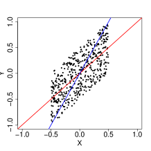
((a)) DAG $X\to Y$

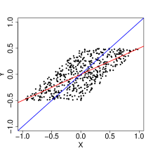
((b)) DAG $Y\to X$

Figure 6. Simulated data from linear structural equation models with uniform errors. Red lines indicate the regression of $Y$ on $X$, while blue lines indicate the regression of $X$ on $Y$.

Such ideas were first used for linear SEMs with non-Gaussian noise, or equivalently, for Linear Non-Gaussian Acyclic Models (LiNGAM) (Shimizu et al., 2006). Recall from Example 2.7 that a linear SEM can be written as $X=(I-B)^{-1}\epsilon$, meaning that $X$ is a linear, invertible mixture of independent errors with mixing matrix $A=(I-B)^{-1}$. In the case of non-Gaussian errors, independent component analysis can identify $A$ up to scaling and permutation of the columns. This idea forms the basis of the original LiNGAM algorithm. Shimizu et al. (2011) give a more advanced implementation that is suitable for larger numbers of variables. The LiNGAM approach has also been extended to allow for latent variables, time series data and feedback loops; see Shimizu (2014) for an overview.

Identifiability of the DAG can also be achieved by various other restrictions on SEMs with additive noise, such as non-linear structural equations (Hoyer et al., 2009), additive models (Bühlmann et al., 2014), or equal error variances (Peters & Bühlmann, 2014).

5. Latent Variables

The methods discussed so far rely on data being available for all relevant variables. However, many applications of graphical models involve latent, i.e., unobserved variables. Sometimes, these are specific variables of interest, e.g., features of extinct species in phylogenetics. In other settings, there may simply be a concern that observed correlations are induced by latent variables. We will review some of the ideas proposed to address this latter issue.

5.1. Low-Rank Structure in Undirected Graphical Models

Let $X=(X_{v}:v\in V)$ be multivariate normal with covariance matrix $\Sigma$, and let $K=\Sigma^{-1}$. Suppose only the variables indexed by $O\subsetneq V$ are observed. Letting $H=V\setminus O$, we have that $X_{O}=(X_{v}:v\in O)$ is multivariate normal with inverse covariance matrix

(5.1) $$\left(\Sigma_{O,O}\right)^{-1}\;=\;K_{O,O}-K_{O,H}\left(K_{H,H}\right)^{-1}K_{H,O}.$$

If $X$ satisfies the Markov property with respect to an undirected graph $G=(V,E)$, then the matrix $K_{O,O}$ is supported over the induced subgraph $G_{O}$, i.e., the $(v,w)$ entry of $K_{O,O}$ is nonzero only if $v=w$ or $v-w\in E$. In contrast, the matrix $K_{O,H}\left(K_{H,H}\right)^{-1}K_{H,O}$ will typically be dense as its $(v,w)$ entry is generically nonzero whenever the graph $G$ contains a path $v-h_{1}-\dots-h_{k}-w$ with $h_{1},\dots,h_{k}\in H$. However, $K_{O,H}\left(K_{H,H}\right)^{-1}K_{H,O}$ has rank at most $|H|$. Therefore, if $G_{O}$ is sparse and the number of latent variables is small, then the inverse covariance matrix of $X_{O}$ is the sum of a sparse and a low-rank matrix.

Example 5.1.

Taking up Example 2.2, let $(X_{1},\dots,X_{5})$ be multivariate normal with the graph from Figure 3 as conditional independence graph. Let $K=(\kappa_{vw})$ be the inverse covariance matrix. If $O=\{1,2,4,5\}$ and $H=\{3\}$, then $X_{O}$ has inverse covariance matrix

$$\begin{pmatrix}\kappa_{11}&\kappa_{12}&0&0\\ \kappa_{12}&\kappa_{22}&0&0\\ 0&0&\kappa_{44}&\kappa_{45}\\ 0&0&\kappa_{45}&\kappa_{55}\\ \end{pmatrix}-\frac{1}{\kappa_{33}}\begin{pmatrix}\kappa_{13}\\ \kappa_{23}\\ \kappa_{34}\\ 0\\ \end{pmatrix}\begin{pmatrix}\kappa_{13}\\ \kappa_{23}\\ \kappa_{34}\\ 0\\ \end{pmatrix}^{T}.$$

Here, the first matrix is sparse and supported over the subgraph with node 3 removed, and the second matrix has rank $|H|=1$. In this example, the low-rank matrix has two zero entries corresponding to the pairs $(X_{1},X_{5})$ and $(X_{2},X_{5})$. This can be seen from the global Markov property because $X_{5}$ can be separated from $(X_{1},X_{2})$ by the observed variable $X_{4}$.

Suppose we have an i.i.d. sample of size $n$ from the distribution of $X_{O}$, with sample covariance matrix $S$, and wish to learn (i) the edges between nodes $v,w\in O$ in the conditional independence graph of $X=(X_{O},X_{H})$ and (ii) the number of latent variables $|H|$. By (5.1), both tasks can be solved simultaneously by estimating a ‘sparse plus low-rank’ decomposition of the inverse covariance matrix of $X_{O}$. Chandrasekaran et al. (2012) propose a penalized maximum likelihood approach in which one solves

(5.2) $$\min_{K^{\rm sp},K^{\rm lr}}\;\Big{\{}-\log\det(K^{\rm sp}-K^{\rm lr})+\text{tr}\left[S(K^{\rm sp}-K^{\rm lr})\right]+\lambda\left[\gamma\|K^{\rm sp}\|_{1}+\text{tr}(K^{\rm lr})\right]\Big{\}},$$

subject to $K^{\rm sp}-K^{\rm lr}$ being positive definite and $K^{\rm lr}$ being positive semidefinite. Here, $K^{\rm sp}$ and $K^{\rm lr}$ stand for the sparse and low rank components of $K$, and have corresponding $\ell_{1}$- and trace/nuclear norm penalties. For tuning parameters $\lambda,\gamma\geq 0$, this optimization problem is convex. Let $(\hat{K}^{\rm sp},\hat{K}^{\rm lr})$ be a minimizer. Chandrasekaran et al. (2012) show that under identifiability conditions the sparsity pattern of $\hat{K}^{\rm sp}$ and the rank of $\hat{K}^{\rm lr}$ consistently estimate the subgraph $G_{O}$ and the number of hidden variables. The theory covers settings in which $|O|$ may roughly be as large as $n$. Possible modifications of the procedure were proposed in discussion pieces published along with Chandrasekaran et al. (2012). Larger instances of (5.2) can be solved using an ADMM algorithm (Ma et al., 2013).

The Gaussian example we treated is only one very special case of graphical modeling with latent variables. Indeed, many mixture and latent factor models can be thought of as graphical models with latent variables. Nevertheless, the example illustrates a general phenomenon: latent variables induce low-rank structure in tensors of moments. This fact is exploited also in methods of Anandkumar et al. (2014) and Chaganty & Liang (2014).

5.2. Latent Variables in Directed Graphical Models

If a DAG model has latent variables, then the marginal distribution of the observed variables can generally not be represented by a DAG. Moreover, if the marginal distribution can be represented by a DAG, this DAG may have no causal interpretation.

Example 5.2.

Let the DAG $G$: $1\to 2\leftarrow 3\to 4\leftarrow 5$ be a perfect map of the distribution of $(X_{1},\dots,X_{5})$, and suppose that $X_{3}$ is latent. There is no DAG on $\{1,2,4,5\}$ that encodes exactly the same d-separation relations among $\{1,2,4,5\}$ as $G$. Hence, there does not exist a perfect map of the marginal distribution of $(X_{1},X_{2},X_{4},X_{5})$.

Example 5.3.

Let the DAG $G$: $1\leftarrow 2\rightarrow 3\leftarrow 4\rightarrow 5$ be a perfect map of the distribution of $(X_{1},\dots,X_{5})$, and suppose that $X_{2}$ and $X_{4}$ are latent. The only conditional independence among the observed variables is $X_{1}\mathchoice{\mathrel{\hbox to0.0pt{$\displaystyle\perp$\hss}\mkern 3.0mu{\displaystyle\perp}}}{\mathrel{\hbox to0.0pt{$\textstyle\perp$\hss}\mkern 3.0mu{\textstyle\perp}}}{\mathrel{\hbox to0.0pt{$\scriptstyle\perp$\hss}\mkern 3.0mu{\scriptstyle\perp}}}{\mathrel{\hbox to0.0pt{$\scriptscriptstyle\perp$\hss}\mkern 3.0mu{\scriptscriptstyle\perp}}}X_{5}$, which is encoded by the DAG $G^{\prime}$: $1\to 3\leftarrow 5$. Indeed, $G^{\prime}$ is a perfect map of the distribution of $X=(X_{1},X_{3},X_{5})$ and would be found when applying consistent methods such as the PC algorithm to a large sample of $(X_{1},X_{3},X_{5})$. However, $G^{\prime}$ does not reflect the causal interpretation of $G$. For example, $G^{\prime}$ suggests $X_{1}$ as a cause of $X_{3}$, but there is no directed path from $X_{1}$ to $X_{3}$ in $G$.

Mixed graphs provide a useful approach to address these problems without explicit modeling of latent variables (e.g., Pearl, 2009; Spirtes et al., 2000; Wermuth, 2011). The nodes of these graphs index the observed variables only. The edges, however, may be of two types, directed and bidirected. This added flexibility allows one to represent the more complicated dependence structures arising from a DAG with latent variables. A straightforward generalization of d-separation determines conditional independencies in mixed graph models. For instance, the mixed graph $1\to 2\longleftrightarrow 4\leftarrow 5$ is a perfect map for the distribution in Example 5.2.

To facilitate constraint-based structure learning in settings with latent variables, Richardson & Spirtes (2002) introduce a class of mixed graphs known as maximal ancestral graphs (MAGs). Every DAG $G=(V,E)$ with $V=O\cup H$, where $O$ and $H$ index the observed and latent variables, respectively, can be transformed into a unique MAG on $O$ such that conditional independencies among the observed variables are preserved. The MAG also encodes ancestral relationships in the underlying DAG $G$, as follows. If the MAG has edge $v\to w$, then $v\in\operatorname{an}_{G}(w)$ but $w\notin\operatorname{an}_{G}(v)$. Similarly, $v\leftrightarrow w$ encodes $v\notin\operatorname{an}_{G}(w)$ and $w\notin\operatorname{an}_{G}(v)$. In general, several MAGs may describe the same set of conditional independencies. The resulting Markov equivalence class of MAGs can be described by a Partial Ancestral Graph (PAG) (Ali et al., 2009).

PAGs can be learned by a generalization of the PC algorithm, called the FCI algorithm (Spirtes et al., 1999; Richardson & Spirtes, 2002). As noted in Section 4.3, the PC algorithm is of polynomial time for graphs of bounded degree, by exploiting the fact that the edge $v-w$ is absent in the skeleton of the DAG $G$ if and only if $X_{v}\mathchoice{\mathrel{\hbox to0.0pt{$\displaystyle\perp$\hss}\mkern 3.0mu{\displaystyle\perp}}}{\mathrel{\hbox to0.0pt{$\textstyle\perp$\hss}\mkern 3.0mu{\textstyle\perp}}}{\mathrel{\hbox to0.0pt{$\scriptstyle\perp$\hss}\mkern 3.0mu{\scriptstyle\perp}}}{\mathrel{\hbox to0.0pt{$\scriptscriptstyle\perp$\hss}\mkern 3.0mu{\scriptscriptstyle\perp}}}X_{w}\,|\,X_{\operatorname{pa}_{G}(v)}$ or $X_{v}\mathchoice{\mathrel{\hbox to0.0pt{$\displaystyle\perp$\hss}\mkern 3.0mu{\displaystyle\perp}}}{\mathrel{\hbox to0.0pt{$\textstyle\perp$\hss}\mkern 3.0mu{\textstyle\perp}}}{\mathrel{\hbox to0.0pt{$\scriptstyle\perp$\hss}\mkern 3.0mu{\scriptstyle\perp}}}{\mathrel{\hbox to0.0pt{$\scriptscriptstyle\perp$\hss}\mkern 3.0mu{\scriptscriptstyle\perp}}}X_{w}\,|\,X_{\operatorname{pa}_{G}(w)}$. In the presence of latent variables, this fact no longer holds. The FCI algorithm therefore performs additional tests, and the number of such tests can be exponential in the number of nodes, even for sparse graphs. The FCI algorithm also uses more complicated orientation rules, which were extended and proved to be complete by Zhang (2008). Colombo et al. (2012) and Claassen et al. (2013) introduce fast modifications of the FCI algorithm that are of polynomial time for graphs of bounded degree.

While MAGs can represent all conditional independencies in the marginal distribution of the observed variables, there can be equality and inequality constraints that MAGs cannot represent. An example is the so-called Verma constraint (Verma & Pearl, 1991); see also Example 3.3.14 in Drton et al. (2009). To represent constraints beyond conditional independencies, there is current work on new classes of graphs, including nested Markov models (Shpitser et al., 2012, 2014) and mDAGs (Evans, 2016).

6. Heterogeneous Data

Heterogeneous data that do not form an i.i.d. sample from a single population are encountered, for instance, in gene expression studies involving different organisms or experimental conditions, or in the comparative analysis of brain networks for patients with different neurological disorders. In such settings, it is of interest to learn the structure of graphical models for subpopulations. More generally, a graph may depend on covariates.

Guo et al. (2011) propose an extension of the graphical lasso from (3.3) to estimate undirected conditional independence graphs of several related Gaussian populations. The authors sum up the log-likelihood functions for $m$ populations with inverse covariance matrices $K_{1},\dots,K_{m}\in\mathbb{R}^{V\times V}$ and then add a sparsity-inducing penalty. To share common structure, the inverse covariances are reparametrized as $K_{i,vw}=\theta_{vw}\gamma_{i,vw}$. The penalty then adds the (vector) $\ell_{1}$ norms of the matrix $(\theta_{vw})$ and the $m$ matrices $(\gamma_{i,vw})$. Sparsity in an estimate of $(\theta_{vw})$ results in edges being simultaneously absent from all $m$ graph estimates, each of which may have further edges absent through zero estimates of $\gamma_{i,vw}$. A downside of this method is that its optimization problem is not convex. Danaher et al. (2014) propose instead the use of group or fused lasso penalties specified in terms of the inverse covariances. The group lasso penalty takes the form $\sum_{v\not=w}\sqrt{K_{1,vw}^{2}+\dots+K_{m,vw}^{2}}$ and leads to edges being simultaneously absent from all $m$ graph estimates; a version of this approach that separates positive from negative signals was also proposed by Chiquet et al. (2011). The fused lasso penalty $\sum_{1\leq i<j\leq m}\sum_{v,w}|K_{i,vw}-K_{j,vw}|$ yields pairwise similar edge patterns in the different populations. Yang et al. (2015b) consider generalizations of this fused lasso penalty and characterize when the resulting optimization problem can be decomposed into smaller problems arising from block-diagonal inverse covariance matrices. Saegusa & Shojaie (2016) treat settings in which some populations may be more closely related than others. Finally, Zhao et al. (2014) show how the difference between two conditional independence graphs can be estimated without estimating the two graphs.

Heterogeneous data also arise from time-course observations, for which we may wish to learn time-varying structure. Zhou et al. (2010) compute glasso estimates at different time points, taking as input a weighted sample covariance matrix that is a kernel estimate of the covariance matrix at time $t$. Alternatively, Kolar et al. (2010) and Kolar & Xing (2012) use fused lasso penalties. Matrix/tensor-normal models, in which one of the dimensions could be time, constitute another approach; see He et al. (2014) and references therein.

Similar issues arise for directed graphical models. In particular, so-called dynamic Bayesian networks have long been used to model temporal dependencies, and there is a natural connection to vector-autoregressive processes in the time series literature (e.g., Shojaie & Michailidis, 2010). A detailed discussion is beyond the scope of this paper.

Finally, we note that heterogeneity from different experimental conditions can also be exploited in structure learning for directed graphical models (Danks et al., 2009; Hauser & Bühlmann, 2012; Hyttinen et al., 2012; Triantafillou & Tsamardinos, 2015). These papers generally assume to have i.i.d. observations from various known experimental conditions, and some of them allow cycles and/or latent variables. Peters et al. (2016) study a scenario where data may come from different experimental conditions, but these conditions are unknown. They provide a method built on the idea that a variable can be well predicted from its causes across different experimental conditions.

7. Discussion

Stimulated to a large extent by applications in gene expression analysis, the field of structure learning in graphical modeling has undergone rapid development, with much of the new work focusing on high-dimensional problems. In this review, we treated some of the main ideas behind these developments, including $\ell_{1}$-regularization techniques, greedy search approaches and methods based on conditional independence tests. Extensions to cope with latent variables have long been of interest and continue to be addressed in new ways. More recently, challenges arising in connection with heterogeneous and dependent data have inspired methods that generalize those for i.i.d. data. Similarly, methods for continuous but non-Gaussian data are an active area of research.

In a different vein, it is of interest to provide an uncertainty assessment for estimates of graph structure. Bayesian approaches naturally include an uncertainty assessment but frequentist techniques that are able to cope with high-dimensional data are also being developed (Janková & van de Geer, 2015; Ren et al., 2015; Xia et al., 2015).

Finally, our treatment of directed graphical models considered acyclic graphs, in which no feedback loops exist in the cause-effect relationships that the model captures. Effective methods for structure learning exist for the acyclic case, but coping with feedback loops is a far more difficult problem. While certain forms of feedback can be represented in the paradigm of linear structural equation modeling (Spirtes et al., 2000; Mooij & Heskes, 2013) and conditional independence can then be exploited in structure learning (Richardson, 1996), these models can generally not be described using solely conditional independence; see Example 3.6 and Appendix A in Drton (2009). New ideas are still needed to effectively learn cyclic cause-effect relationships from possibly high-dimensional observational data.

References

- Ali et al. (2009) Ali RA, Richardson TS, Spirtes P. 2009. Markov equivalence for ancestral graphs. Ann. Statist. 37:2808–2837
- Anandkumar et al. (2014) Anandkumar A, Ge R, Hsu D, Kakade SM, Telgarsky M. 2014. Tensor decompositions for learning latent variable models. J. Mach. Learn. Res. 15:2773–2832
- Anandkumar & Valluvan (2013) Anandkumar A, Valluvan R. 2013. Learning loopy graphical models with latent variables: efficient methods and guarantees. Ann. Statist. 41:401–435
- Andersson et al. (1997) Andersson SA, Madigan D, Perlman MD. 1997. A characterization of Markov equivalence classes for acyclic digraphs. Ann. Statist. 25:505–541
- Banerjee et al. (2008) Banerjee O, El Ghaoui L, d’Aspremont A. 2008. Model selection through sparse maximum likelihood estimation for multivariate Gaussian or binary data. J. Mach. Learn. Res. 9:485–516
- Banerjee & Ghosal (2015) Banerjee S, Ghosal S. 2015. Bayesian structure learning in graphical models. J. Multivariate Anal. 136:147–162
- Barber & Drton (2015) Barber RF, Drton M. 2015. High-dimensional Ising model selection with Bayesian information criteria. Electron. J. Stat. 9:567–607
- Besag (1975) Besag J. 1975. Statistical analysis of non-lattice data. J. R. Stat. Soc. Ser. D. The Statistician 24:179–195
- Bilodeau (2014) Bilodeau M. 2014. Graphical lassos for meta-elliptical distributions. Canad. J. Statist. 42:185–203
- Bollen (1989) Bollen KA. 1989. Structural equations with latent variables. John Wiley & Sons, New York
- Bresler (2015) Bresler G. 2015. Efficiently learning Ising models on arbitrary graphs. In Proc. 47th Symp. Theory of Comp. (STOC’15). New York, NY: ACM, 771–782
- Bühlmann et al. (2014) Bühlmann P, Peters J, Ernest J. 2014. CAM: causal additive models, high-dimensional order search and penalized regression. Ann. Statist. 42:2526–2556
- Cai et al. (2011) Cai T, Liu W, Luo X. 2011. A constrained minimization approach to sparse precision matrix estimation. J. Amer. Statist. Assoc. 106:594–607
- Cai et al. (2016) Cai TT, Liu W, Zhou HH. 2016. Estimating sparse precision matrix: Optimal rates of convergence and adaptive estimation. Ann. Statist. 44:455–488
- Chaganty & Liang (2014) Chaganty AT, Liang P. 2014. Estimating latent-variable graphical models using moments and likelihoods. In Proc. 31st Int. Conf. Mach. Learn. (ICML’14). 1872–1880
- Chandrasekaran et al. (2012) Chandrasekaran V, Parrilo PA, Willsky AS. 2012. Latent variable graphical model selection via convex optimization. Ann. Statist. 40:1935–1967
- Chen et al. (2015) Chen S, Witten DM, Shojaie A. 2015. Selection and estimation for mixed graphical models. Biometrika 102:47–64
- Chickering (2002) Chickering DM. 2002. Optimal structure identification with greedy search. J. Mach. Learn. Res. 3:507–554
- Chickering & Meek (2015) Chickering DM, Meek C. 2015. Selective Greedy Equivalence Search: finding optimal Bayesian networks using a polynomial number of score evaluations. In Proc. 31st Conf. on Uncert. in Artif. Intell. (UAI’15). Corvallis, OR: AUAI Press, 211–219
- Chiquet et al. (2011) Chiquet J, Grandvalet Y, Ambroise C. 2011. Inferring multiple graphical structures. Stat. Comput. 21:537–553
- Chow & Liu (1968) Chow CK, Liu C. 1968. Approximating discrete probability distributions with dependence trees. IEEE Trans. Inf. Theory IT-14:462––467
- Claassen et al. (2013) Claassen T, Mooij JM, Heskes T. 2013. Learning sparse causal models is not NP-hard. In Proc. 29th Conf. Uncert. Artif. Intell. (UAI’13). Corvallis, OR: AUAI Press, 172–181
- Colombo & Maathuis (2014) Colombo D, Maathuis MH. 2014. Order-independent constraint-based causal structure learning. J. Mach. Learn. Res. 15:3741–3782
- Colombo et al. (2012) Colombo D, Maathuis MH, Kalisch M, Richardson TS. 2012. Learning high-dimensional directed acyclic graphs with latent and selection variables. Ann. Statist. 40:294–321
- Cussens & Bartlett (2013) Cussens J, Bartlett M. 2013. Advances in Bayesian network learning using integer programming. In Proc. 29th Conf. Uncert. Artif. Intell. (UAI’13). Corvallis, OR: AUAI Press, 182–191
- Danaher et al. (2014) Danaher P, Wang P, Witten DM. 2014. The joint graphical lasso for inverse covariance estimation across multiple classes. J. R. Stat. Soc. Ser. B. Stat. Methodol. 76:373–397
- Danks et al. (2009) Danks D, Glymour C, Tillman RE. 2009. Integrating locally learned causal structures with overlapping variables. In Adv. Neural Inf. Proc. Syst. 21 (NIPS’09). Curran Associates, 1665–1672
- Dasarathy et al. (2016) Dasarathy G, Singh A, Balcan MF, Park JH. 2016. Active learning algorithms for graphical model selection. ArXiv:1602.00354
- de Campos et al. (2009) de Campos C, Zeng Z, Ji Q. 2009. Structure learning of Bayesian networks using constraints. In Proc. 26th Int. Conf. Mach. Learn. (ICML’09). Omnipress, 113–120
- Defazio & Caetano (2012) Defazio A, Caetano TS. 2012. A convex formulation for learning scale-free networks via submodular relaxation. In Adv. Neural Inf. Proc. Syst. 25 (NIPS’12). Curran Associates, 1250–1258
- Didelez (2016) Didelez V. 2016. Graphical models for dynamic processes. Forthcoming
- Drton (2009) Drton M. 2009. Likelihood ratio tests and singularities. Ann. Statist. 37:979–1012
- Drton & Perlman (2007) Drton M, Perlman MD. 2007. Multiple testing and error control in Gaussian graphical model selection. Statist. Sci. 22:430–449
- Drton et al. (2009) Drton M, Sturmfels B, Sullivant S. 2009. Lectures on algebraic statistics, vol. 39 of Oberwolfach Seminars. Birkhäuser Verlag, Basel
- Edwards et al. (2010) Edwards D, de Abreu GC, Labouriau R. 2010. Selecting high-dimensional mixed graphical models using minimal AIC or BIC forests. BMC Bioinformatics 11:1–13
- Evans (2016) Evans RJ. 2016. Graphs for margins of bayesian networks. Scand. J. Statist. Forthcoming
- Fan et al. (2016) Fan J, Liu H, Ning Y, Zou H. 2016. High dimensional semiparametric latent graphical model for mixed data. J. R. Stat. Soc. Ser. B. Stat. Methodol. :n/a–n/a
- Finegold & Drton (2011) Finegold M, Drton M. 2011. Robust graphical modeling of gene networks using classical and alternative -distributions. Ann. Appl. Stat. 5:1057–1080
- Finegold & Drton (2014) Finegold M, Drton M. 2014. Robust Bayesian graphical modeling using Dirichlet -distributions. Bayesian Anal. 9:521–550
- Forbes & Lauritzen (2015) Forbes PGM, Lauritzen S. 2015. Linear estimating equations for exponential families with application to Gaussian linear concentration models. Linear Algebra Appl. 473:261–283
- Foygel & Drton (2010) Foygel R, Drton M. 2010. Extended Bayesian information criteria for Gaussian graphical models. Adv. Neural Inf. Process. Syst. 23:2020–2028
- Friedman et al. (2008) Friedman J, Hastie T, Tibshirani R. 2008. Sparse inverse covariance estimation with the graphical lasso. Biostatistics 9:432–441
- Friedman (2004) Friedman N. 2004. Inferring cellular networks using probabilistic graphical models. Science 303:799
- Friedman et al. (2002) Friedman N, Ninio M, Pe’er I, Pupko T. 2002. A structural em algorithm for phylogenetic inference. Journal of Computational Biology 9:331–353
- Frydenberg (1990) Frydenberg M. 1990. The chain graph Markov property. Scand. J. Statist. 17:333–353
- Gao et al. (2012) Gao X, Pu DQ, Wu Y, Xu H. 2012. Tuning parameter selection for penalized likelihood estimation of Gaussian graphical model. Statist. Sinica 22:1123–1146
- Geiger et al. (2006) Geiger D, Meek C, Sturmfels B. 2006. On the toric algebra of graphical models. Ann. Statist. 34:1463–1492
- Guo et al. (2011) Guo J, Levina E, Michailidis G, Zhu J. 2011. Joint estimation of multiple graphical models. Biometrika 98:1–15
- Harris & Drton (2013) Harris N, Drton M. 2013. PC algorithm for nonparanormal graphical models. J. Mach. Learn. Res. 14:3365–3383
- Hauser & Bühlmann (2012) Hauser A, Bühlmann P. 2012. Characterization and greedy learning of interventional Markov equivalence classes of directed acyclic graphs. J. Mach. Learn. Res. 13:2409–2464
- He et al. (2014) He S, Yin J, Li H, Wang X. 2014. Graphical model selection and estimation for high dimensional tensor data. J. Multivariate Anal. 128:165–185
- He et al. (2013) He Y, Jia J, Yu B. 2013. Reversible MCMC on Markov equivalence classes of sparse directed acyclic graphs. Ann. Statist. 41:1742–1779
- Höfling & Tibshirani (2009) Höfling H, Tibshirani R. 2009. Estimation of sparse binary pairwise Markov networks using pseudo-likelihoods. J. Mach. Learn. Res. 10:883–906
- Højsgaard et al. (2012) Højsgaard S, Edwards D, Lauritzen S. 2012. Graphical models with R. Use R! Springer, New York
- Hoyer et al. (2009) Hoyer PO, Janzing D, Mooij J, Peters J, Schölkopf B. 2009. Nonlinear causal discovery with additive noise models. In Adv. Neural Inf. Proc. Syst. 21 (NIPS’08). 689–696
- Hsieh et al. (2013) Hsieh CJ, Sustik MA, Dhillon IS, Ravikumar PK, Poldrack R. 2013. Big & quic: Sparse inverse covariance estimation for a million variables. In Adv. Neural Inf. Proc. Syst. 26 (NIPS’13). Curran Associates, Inc., 3165–3173
- Hyttinen et al. (2012) Hyttinen A, Eberhardt F, Hoyer P. 2012. Causal discovery of linear cyclic models from multiple experimental data sets with overlapping variables. In Proc. 28th Conf. Uncert. Artif. Intell. (UAI’12). Corvallis, Oregon: AUAI Press, 387–396
- Hyvärinen (2005) Hyvärinen A. 2005. Estimation of non-normalized statistical models by score matching. J. Mach. Learn. Res. 6:695–709
- Hyvärinen (2007) Hyvärinen A. 2007. Some extensions of score matching. Comput. Statist. Data Anal. 51:2499–2512
- Jaakkola et al. (2010) Jaakkola T, Sontag D, Globerson A, Meila M. 2010. Learning bayesian network structure using lp relaxations. J. Mach. Learn. Res. W&CP 9:358–365. AISTATS 2010
- Jalali et al. (2011) Jalali A, Johnson CC, Ravikumar PK. 2011. On learning discrete graphical models using greedy methods. In Adv. Neural Inf. Proc. Syst. 24 (NIPS’11). Curran Associates, 1935–1943
- Janková & van de Geer (2015) Janková J, van de Geer S. 2015. Confidence intervals for high-dimensional inverse covariance estimation. Electron. J. Stat. 9:1205–1229
- Janofsky (2015) Janofsky E. 2015. Exponential series approaches for nonparametric graphical models. Ph.D. thesis, The University of Chicago. ArXiv:1506.03537
- Kalisch & Bühlmann (2007) Kalisch M, Bühlmann P. 2007. Estimating high-dimensional directed acyclic graphs with the PC-algorithm. J. Mach. Learn. Res. 8:613–636
- Karger & Srebro (2001) Karger D, Srebro N. 2001. Learning Markov networks: Maximum bounded tree-width graphs. In Proc. 12th ACM-SIAM Symp. on Discrete Algorithms. 392–401
- Khare et al. (2015) Khare K, Oh SY, Rajaratnam B. 2015. A convex pseudolikelihood framework for high dimensional partial correlation estimation with convergence guarantees. J. R. Stat. Soc. Ser. B. Stat. Methodol. 77:803–825
- Kolar et al. (2010) Kolar M, Song L, Ahmed A, Xing EP. 2010. Estimating time-varying networks. Ann. Appl. Stat. 4:94–123
- Kolar & Xing (2012) Kolar M, Xing EP. 2012. Estimating networks with jumps. Electron. J. Stat. 6:2069–2106
- Koller & Friedman (2009) Koller D, Friedman N. 2009. Probabilistic graphical models. Adaptive Computation and Machine Learning. MIT Press, Cambridge, MA. Principles and techniques
- Lauritzen (1996) Lauritzen SL. 1996. Graphical models, vol. 17 of Oxford Statistical Science Series. The Clarendon Press, Oxford University Press, New York. Oxford Science Publications
- Lederer & Müller (2014) Lederer J, Müller C. 2014. Topology adaptive graph estimation in high dimensions. ArXiv:1410.7279
- Lin et al. (2016) Lin L, Drton M, Shojaie A. 2016. Estimation of high-dimensional graphical models using regularized score matching. Electron. J. Stat. 10:806–854
- Liu et al. (2012a) Liu H, Han F, Yuan M, Lafferty J, Wasserman L. 2012a. High-dimensional semiparametric Gaussian copula graphical models. Ann. Statist. 40:2293–2326
- Liu et al. (2012b) Liu H, Han F, Zhang CH. 2012b. Transelliptical graphical models. In Adv. Neural Inf. Proc. Syst. 25 (NIPS’12). 809–817
- Liu et al. (2009) Liu H, Lafferty J, Wasserman L. 2009. The nonparanormal: semiparametric estimation of high dimensional undirected graphs. J. Mach. Learn. Res. 10:2295–2328
- Liu et al. (2010) Liu H, Roeder K, Wasserman L. 2010. Stability approach to regularization selection (StARS) for high-dimensional graphical models. In Adv. Neural Inf. Process. Syst. 23 (NIPS’10). 1432–1440
- Liu et al. (2011) Liu H, Xu M, Gu H, Gupta A, Lafferty J, Wasserman L. 2011. Forest density estimation. J. Mach. Learn. Res. 12:907–951
- Liu (2013) Liu W. 2013. Gaussian graphical model estimation with false discovery rate control. Ann. Statist. 41:2948–2978
- Liu & Luo (2015) Liu W, Luo X. 2015. Fast and adaptive sparse precision matrix estimation in high dimensions. J. Multivariate Anal. 135:153–162
- Ma et al. (2013) Ma S, Xue L, Zou H. 2013. Alternating direction methods for latent variable Gaussian graphical model selection. Neural Comput. 25:2172–2198
- Maathuis et al. (2010) Maathuis MH, Colombo D, Kalisch M, Bühlmann P. 2010. Predicting causal effects in large-scale systems from observational data. Nat. Methods 7:247–248
- Maathuis et al. (2009) Maathuis MH, Kalisch M, Bühlmann P. 2009. Estimating high-dimensional intervention effects from observational data. Ann. Statist. 37:3133–3164
- Marbach et al. (2012) Marbach D, Costello JC, Kuffner R, Vega NM, Prill RJ, et al. 2012. Wisdom of crowds for robust gene network inference. Nature Methods 9:796–804
- Matúš (2012) Matúš F. 2012. On conditional independence and log-convexity. Ann. Inst. Henri Poincaré Probab. Stat. 48:1137–1147
- Mazumder & Hastie (2012a) Mazumder R, Hastie T. 2012a. Exact covariance thresholding into connected components for large-scale graphical lasso. J. Mach. Learn. Res. 13:781–794
- Mazumder & Hastie (2012b) Mazumder R, Hastie T. 2012b. The graphical lasso: new insights and alternatives. Electron. J. Stat. 6:2125–2149
- Meinshausen (2008) Meinshausen N. 2008. A note on the Lasso for Gaussian graphical model selection. Statist. Probab. Lett. 78:880–884
- Meinshausen & Bühlmann (2006) Meinshausen N, Bühlmann P. 2006. High-dimensional graphs and variable selection with the lasso. Ann. Statist. 34:1436–1462
- Meinshausen & Bühlmann (2010) Meinshausen N, Bühlmann P. 2010. Stability selection. J. R. Stat. Soc. Ser. B Stat. Methodol. 72:417–473
- Mitra et al. (2016) Mitra R, Müller P, Ji Y. 2016. Bayesian Graphical Models for Differential Pathways. Bayesian Anal. 11:99–124
- Mooij & Heskes (2013) Mooij JM, Heskes T. 2013. Cyclic causal discovery from continuous equilibrium data. In Proc. 29th Conf. Uncert. Artif. Intell. (UAI’13). AUAI Press, 431–439
- Nandy et al. (2016a) Nandy P, Hauser A, Maathuis MH. 2016a. High-dimensional consistency in score-based and hybrid structure learning. ArXiv:1507.02608
- Nandy et al. (2016b) Nandy P, Maathuis MH, Richardson TS. 2016b. Estimating the effect of joint interventions from observational data in sparse high-dimensional settings. Ann. Statist. Forthcoming
- Neapolitan (2004) Neapolitan RE. 2004. Learning bayesian networks. Prentice Hall series in artificial intelligence. Upper Saddle River, NJ: Pearson Prentice Hall
- Nyman et al. (2014) Nyman H, Pensar J, Koski T, Corander J. 2014. Stratified graphical models—context-specific independence in graphical models. Bayesian Anal. 9:883–908
- Parviainen & Koivisto (2009) Parviainen P, Koivisto M. 2009. Exact structure discovery in bayesian networks with less space. In Proc. 25th Conf. Uncert. Artif. Intell. (UAI’09). Arlington, VA: AUAI Press, 436–443
- Pearl (2009) Pearl J. 2009. Causality. Cambridge University Press, Cambridge, 2nd ed. Models, reasoning, and inference
- Perković et al. (2015) Perković E, Textor J, Kalisch M, Maathuis MH. 2015. A complete adjustment criterion. In Proc. 31st Conf. Uncert. Artif. Intell. (UAI’15). Corvallis, OR: AUAI Press, 682–691
- Peters & Bühlmann (2014) Peters J, Bühlmann P. 2014. Identifiability of Gaussian structural equation models with equal error variances. Biometrika 101:219–228
- Peters et al. (2016) Peters J, Bühlmann P, Meinshausen N. 2016. Causal inference using invariant prediction: identification and confidence intervals. J. R. Stat. Soc. Ser. B. Stat. Methodol. Forthcoming
- Peterson et al. (2015) Peterson C, Stingo FC, Vannucci M. 2015. Bayesian inference of multiple Gaussian graphical models. J. Amer. Statist. Assoc. 110:159–174
- Ravikumar et al. (2010) Ravikumar P, Wainwright MJ, Lafferty JD. 2010. High-dimensional Ising model selection using -regularized logistic regression. Ann. Statist. 38:1287–1319
- Ravikumar et al. (2011) Ravikumar P, Wainwright MJ, Raskutti G, Yu B. 2011. High-dimensional covariance estimation by minimizing -penalized log-determinant divergence. Electron. J. Stat. 5:935–980
- Ray et al. (2015) Ray A, Sanghavi S, Shakkottai S. 2015. Improved greedy algorithms for learning graphical models. IEEE Trans. Inform. Theory 61:3457–3468
- Ren et al. (2015) Ren Z, Sun T, Zhang CH, Zhou HH. 2015. Asymptotic normality and optimalities in estimation of large Gaussian graphical models. Ann. Statist. 43:991–1026
- Richardson (1996) Richardson T. 1996. A discovery algorithm for directed cyclic graphs. In Proc. 12th Conf. Uncert. Artif. Intell. (UAI’96). AUAI Press, 454–461
- Richardson & Spirtes (2002) Richardson TS, Spirtes P. 2002. Ancestral graph Markov models. Ann. Statist. 30:962–1030
- Roverato (2005) Roverato A. 2005. A unified approach to the characterization of equivalence classes of DAGs, chain graphs with no flags and chain graphs. Scand. J. Statist. 32:295–312
- Saegusa & Shojaie (2016) Saegusa T, Shojaie A. 2016. Joint estimation of precision matrices in heterogeneous populations. ArXiv:1601.00142
- Shah & Samworth (2013) Shah RD, Samworth RJ. 2013. Variable selection with error control: another look at stability selection. J. Roy. Statist. Soc. Ser. B 75:55–80
- Shimizu (2014) Shimizu S. 2014. LiNGAM: Non-Gaussian methods for estimating causal structures. Behaviormetrika 41:65–98
- Shimizu et al. (2006) Shimizu S, Hoyer PO, Hyvärinen A, Kerminen A. 2006. A linear non-Gaussian acyclic model for causal discovery. J. Mach. Learn. Res. 7:2003–2030
- Shimizu et al. (2011) Shimizu S, Inazumi T, Sogawa Y, Hyvärinen A, Kawahara Y, et al. 2011. DirectLiNGAM: a direct method for learning a linear non-Gaussian structural equation model. J. Mach. Learn. Res. 12:1225–1248
- Shojaie & Michailidis (2010) Shojaie A, Michailidis G. 2010. Discovering graphical Granger causality using the truncating lasso penalty. Bioinformatics 26:i517–i523
- Shpitser et al. (2014) Shpitser I, Evans R, Richardson T, Robins J. 2014. Introduction to nested Markov models. Behaviormetrika 41:3–39
- Shpitser et al. (2012) Shpitser I, Richardson TS, Robins JM, Evans R. 2012. Parameter and structure learning in nested Markov models, In UAI Workshop on Causal Structure Learning