Example Demonstrating the Application of Small-gain and Density Propagation Conditions for Interconnections

Abstract

This work provides an example that motivates and illustrates theoretical results related to a combination of small-gain and density propagation conditions. Namely, in case the small-gain fails to hold at certain points or intervals the density propagation condition can be applied to assure global stability properties. We repeat the theoretical results here and demonstrate how they can be applied in the proposed example.

I Introduction

Here we will consider two nonlinear interconnected systems, each of them is ISS, and ask whether the interconnection is ISS as well. Typically one uses the so-called small-gain condition to assure this property. However in case this condition fails to hold at several points or intervals further conditions to assure global stability properties are necessary. This condition can be written in terms of a density propagation inequality [1]. Moreover if one tries to verify the small-gain condition numerically it can easily happen that this condition fails due to the unprecise computer calculations. Also in this case the density propagation condition can help to fill such gaps.

The example considered below demonstrates this kind of situations and illustrates how a combination of small-gain and density propagation conditions can be applied. First we recall the related theoretical results, that will be published elsewhere, then we will consider the example in detail.

II Preliminaries and notation

The notation $\overline{\mathbb{N}}$ (resp. $\overline{\mathbb{R}}$) stands for the set $\mathbb{N}\cup\{\infty\}$ (resp. $\mathbb{R}\cup\{\infty\}$). For a given $a,b\in\overline{\mathbb{R}}$ let $\mathbb{N}_{[a,b]}=\{s\in\overline{\mathbb{N}}:a\leq s\leq b\}$. Let $\mathbf{S}\subset\mathbb{R}^{n}$, its closure (resp. interior) is denoted as $\mathtt{cl}\{\mathbf{S}\}$ (resp. $\operatorname{\mathtt{int}}\{\mathbf{S}\}$). We recall the following standard definitions: a function $\alpha:[0,\infty)\to[0,\infty)$ is of class $\mathcal{K}$ when $\alpha$ is continuous, strictly increasing, and $\alpha(0)=0$. If $\alpha$ is also unbounded, then we say it is of class $\mathcal{K}_{\infty}$. A continuous function $\beta:[0,\infty)\times[0,\infty)\to[0,\infty)$ is of class $\mathcal{KL}$, when $\beta(\cdot,t)$ is of class $\mathcal{K}$ for each fixed $t\geq 0$, and $\beta(r,t)$ decreases to $0$ as $t\to\infty$ for each fixed $r\geq 0$.

Consider the interconnection of two systems $\Sigma_{1}$ and $\Sigma_{2}$

$$\Sigma_{i}:\quad\dot{x}_{i}=f_{i}(x_{1}(t),x_{2}(t),u_{i}(t)),\quad i=1,2$$ (1)

$x_{i}(t)\in\mathbb{R}^{n_{i}}$ is the state of $\Sigma_{i}$ and $u_{i}(t)\in\mathbb{R}^{m_{i}}$ is its external input, $f_{i}$ is assumed to be of class $\mathcal{C}^{1}$ and satisfy $f_{i}(0,0,0)=0$. This interconnection can be written as

$$\dot{x}=f(x(t),u(t))$$ (2)

with the state $x=(x_{1},x_{2})\in\mathbb{R}^{n},\;n=n_{1}+n_{2}$, dynamics $f=(f_{1},f_{2})$ and input $u=(u_{1},u_{2})\in\mathbb{R}^{m},\;m=m_{1}+m_{2}$.

Definition 1 ([2]).

The system (2) is called input-to-state stable (ISS) if there exist functions $\beta\in\mathcal{K}\mathcal{L}$ and $\tilde{\gamma}_{u}\in\mathcal{K}_{\infty}$ such that, for each initial condition $x(0)$ and each measurable essentially bounded input $u(\cdot)$, the solution $x(\cdot)$ of (2) satisfies

$$|x(t)|\leq \beta(|x(0)|,t)+\tilde{\gamma}_{u}(|u|_{\infty})\quad\forall t\geq 0.$$

ISS is equivalent to the existence of an ISS-Lyapunov function, which we define for each subsystem in (1):

Definition 2.

A function $V_{i}\in\mathcal{L}\mathpzc{ip}_{\mathrm{loc}}(\mathbb{R}^{n_{i}},\mathbb{R}_{\geq 0})$ is called storage function if for some $\underline{\alpha}_{i},\overline{\alpha}_{i}\in\mathcal{K}_{\infty}$ it holds that $\underline{\alpha}_{i}(|x_{i}|)\leq V_{i}(x_{i})\leq\overline{\alpha}_{i}(|x_{i}|)\quad\forall x_{i}\in\mathbb{R}^{n_{i}}$.

Definition 3.

A storage function $V_{i}$ is called ISS-Lyapunov function for (1) if for some $\gamma_{i,j},\gamma_{i},\alpha_{i}\in\mathcal{K}_{\infty}$ the implication

$$V_{i}(x_{i})\geq\max\bigg{\{}\gamma_{i,j}(V_{j}(x_{j})),\gamma_{i}(|u_{i}|)\bigg{\}}$$ (3a)

$$\Rightarrow\;\nabla V_{i}(x_{i})\cdot f_{i}(x_{i},x_{j},u_{i})\leq-\alpha_{i}(|x_{i}|).$$ (3b)

holds for each $x_{i}\in\mathbb{R}^{n_{i}}$, $x_{j}\in\mathbb{R}^{n_{j}}$, and $u_{i}\in\mathbb{R}^{m_{i}}$. $\gamma_{i,j}$ (resp. $\gamma_{i}$) is called interconnecting (resp. external) ISS-Lyapunov gain.

Stability of the resulting interconnected system (2) can be deduced from the small-gain theorem [3]: if the interconnecting ISS-Lyapunov gains satisfy

$$\gamma_{12}\circ\gamma_{21}(s)<s\quad\forall s>0,$$ (4)

then system (2) is input-to-state stable.

In this paper we assume that the graphs of $\gamma^{-1}_{12}$ and $\gamma_{21}$ have several points of intersection. It means that small-gain condition does not hold globally and the previously known results cannot be utilized to verify global stability properties of the interconnection. To guarantee the desired stability properties of the interconnection, the dual to Lyapunov’s techniques [1, 4] is employed in specific domains of the state space. Our approach extends the results of [5] to the case of arbitrary number of intersection points of $\gamma^{-1}_{12}$ and $\gamma_{21}$ and allows for external inputs. Moreover our stability conditions are less restrictive then in [5].

Assumption 1.

Let for each $i=1,2$ there exist an ISS-Lyapunov function $V_{i}$ for $\Sigma_{i}$ from (1) with the corresponding gain functions $\gamma_{i,j},\gamma_{i}\in\mathcal{K}_{\infty}$, and $\alpha_{i}\in\mathcal{K}_{\infty}$.

Assumption 2.

Let the intersection points of the graphs of $\gamma^{-1}_{12}$ and $\gamma_{21}$ be given. These points define a sequence of intervals $\mathbf{M}_{k}=(\underline{M}_{k},\overline{M}_{k})$ where the small-gain condition (4) holds for any $s\in\mathbf{M}_{k}$, $k\in\mathbb{N}_{[1,\ell]}$, $\ell\in{\mathbb{N}}$.

For a given $\delta\in\mathbb{R}_{\geq 0}$ let $\mathbf{L}_{i}(\delta)=\{x_{i}\in\mathbb{R}^{n_{i}}:V_{i}(x_{i})\leq\delta\}$.

Theorem 4.

Let Assumptions 1 and 2 hold. Then there exists $\gamma\in\mathcal{K}_{\infty}$ such that almost all solutions to system (2) starting in the set $\mathbf{B}_{k}$ converge to a neighborhood of the set $\mathbf{A}_{k}$ with radius $\gamma(|u|_{\infty})$, where

$$\begin{split}\mathbf{A}_{k}=\{x\in\mathbb{R}^{n}:x_{1}\in\mathbf{L}_{1}(\max\{\underline{M}_{k},\gamma_{12}(\underline{M}_{k})\}),\\ x_{2}\in\mathbf{L}_{2}(\max\{\gamma_{21}(\underline{M}_{k}),\gamma_{21}\circ\gamma_{21}(\underline{M}_{k})\})\},\end{split}$$ (5)

$$\mathbf{B}_{k}=\{x\in\mathbb{R}^{n}:x_{1}\in\mathbf{L}_{1}(\overline{M}_{k}),x_{2}\in\mathbf{L}_{2}(\gamma_{21}(\overline{M}_{k}))\}.$$ (6)

If $\overline{M}_{\ell}\neq\infty$ then the above mentioned convergence holds only for some bounded inputs $u$.

The input-to-state stability of system (2) follows trivially when $\ell=1$, $\underline{M}_{1}=0$, $\overline{M}_{1}=\infty$; then $\mathbf{A}_{1}=\{0\}$ and $\mathbf{B}_{1}=\mathbb{R}^{2}$. However, when $\ell>1$, solutions to (2) starting in the set $\mathbf{A}_{k}$ may converge to an $\omega$-limit set [6, Birkhoff’s Theorem] that lies inside the set $\mathbf{A}_{k}$ and do not converge to a ball centred at the origin whose radius is proportional to the norm of the input. Due to this fact, the next assumption is needed to check the asymptotic behaviour of solutions inside the sets $\mathbf{A}_{k}$. Let $\mathbf{B}_{0}=\emptyset$ and $\mathbf{A}_{\ell+1}=\mathbb{R}^{n}$.

Assumption 3.

Let for each $k\in\mathbb{N}_{[1,\ell+1]}$, there exist an open set $\mathbf{D}_{k}\subset\mathbb{R}^{n}$ satisfying $\{\mathbf{A}_{k}\setminus\mathbf{B}_{k-1}\}\subsetneq\mathtt{cl}\{\mathbf{D}_{k}\}$ and

• A differentiable function $\rho_{k}:\mathbf{D}_{k}\to\mathbb{R}_{>0}$;

• A continuous function $q_{k}:\mathbf{D}_{k}\to\mathbb{R}_{\geq 0}$ such that, for almost every $x\in\mathbf{D}_{k}$, $q_{k}(x)>0$;

• A function $\gamma_{k}\in\mathcal{K}$ such that, for every $x\in\mathbf{D}_{k}$ and for every $u\in\mathbb{R}^{m}$, the following implication holds

  $$\max_{i=1,2}V_{i}(x_{i})\geq\gamma_{k}(|u|)\quad\Rightarrow$$ (7a)

  $$\mathtt{div}(\rho_{k}f)(x,u):=\sum_{j=1}^{n}\tfrac{\partial(\rho_{k}f_{j})}{\partial x_{j}}(x,u)\geq q_{k}(x)$$ (7b)

Definition 5.

[1] The origin is called almost ISS for (2) if it is locally asymptotically stable and for some $\gamma\in\mathcal{K}_{\infty}$

$$\limsup_{t\to\infty}|x(t,x(0),u)|\leq\gamma(|u|_{\infty})$$

holds for every input $u\in\mathcal{L}_{\mathrm{loc}}^{\infty}(\mathbb{R}_{\geq 0},\mathbb{R}^{m})$ and for almost every initial condition $x(0)\in\mathbb{R}^{n}$.

Theorem 6.

Under Assumptions 1, 2, and 3 system (2) is almost input-to-state stable.

III Illustrative example

Let $n\in\mathbb{N}\cup\{\infty\}$ be a constant value. Define the value $a=(4\pi^{2}n+3\pi^{2})/2$ and the functions $g:\mathbb{R}\to\mathbb{R}$ as

$$g(r)= \ \tanh(2r)+\displaystyle\sum_{i=1}^{n}\mathtt{sign}(r)$$

$$\cdot(1+\mathtt{sign}(r)\tanh(2(r-\mathtt{sign}(r)2\pi^{2}i))),$$

for every $$|r|\leq a$$ and

$$g(r)=\mathtt{sign}(r)((2n+1)+(r-\mathtt{sign}(r)a)^{2}),$$ (8)

for every $$|r|>a$$,

and $h:\mathbb{R}\to\mathbb{R}$ as

$$h(r)=\sin^{2}\left(\frac{r}{2\pi}\right)+\displaystyle\sum_{i=1}^{n}(\tanh(r-2\pi^{2}i)+1)\sin^{2}\left(\frac{r}{2\pi}\right).$$

Functions $g$ and $h$ are plotted in Figure 1.

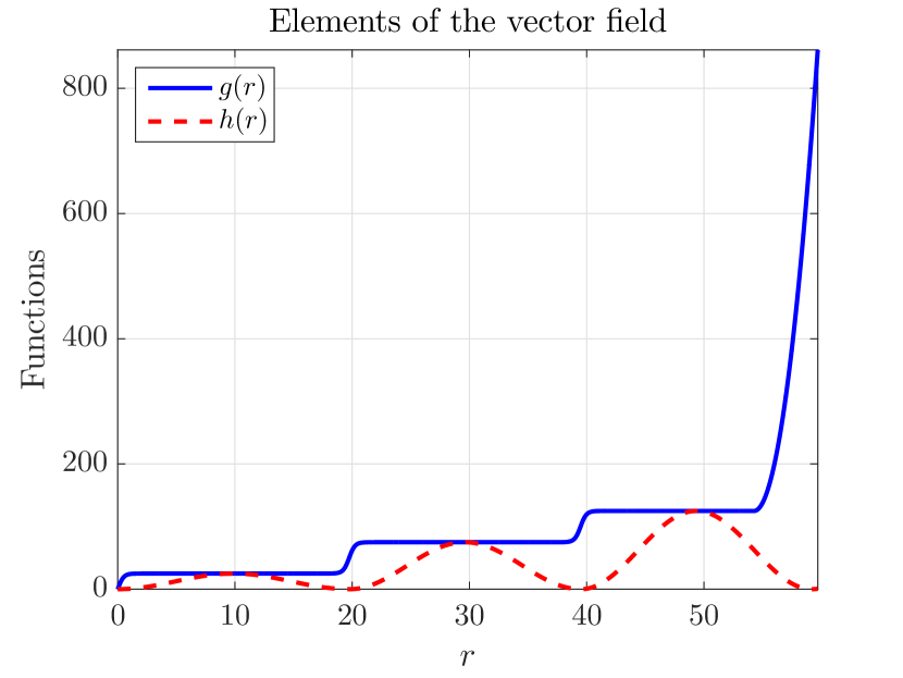
Figure 1: Plot of the functions $g$ and $h$, for $n=2$, and on the interval $[0,1.1\times 11\pi^{2}/2]$.

Although the equation $\tanh(r)-1=0$ has no (finite) solution. For computer programs running with a minimum precision $p$ for number representation there exist values $r>0$ such that, whenever the inequality $|\tanh(r)-1|<p$ is true, this value is rounded to zero. This is denoted as $\mathbin{\mathtt{round}}(\tanh(r)-1)=0$. The values where $r$ satisfies the equation $\mathbin{\mathtt{round}}(\tanh(r)-1)=0$ are said to be regions where $g$ is numerically constant.

For each index $i=1,2$, consider the system defined by

$$\dot{x}_{i}=-\left(25+\frac{|u_{i}|_{\infty}}{a+1}\right)g(x_{i})+25h(x_{3-i})+\left(\frac{|u_{i}|_{\infty}}{a+1}\right)^{2}.$$ (9)

Denote the vector field describing the differential equation (9) by $f_{i}$ and let $f=(f_{1},f_{2})^{\top}$. This system is ISS, as shown below.

Letting either $|u_{i}|_{\infty}=0$ or $n=\infty$, Equation (9) reduces to

$$\dot{x}_{i}=-25g(x_{i})+25h(x_{3-i}).$$ (10)

For values of $a$ that are big enough (even infinite), due to numerical imprecision, the system resulting from the composition of (9) shows the presence of (possibliy infinitely) $(n+1)$ equilibrium points. These points are the maxima of the function $h$, namely, the points $r_{k}=2\pi^{2}k+\pi^{2}$, where $k\in\mathbb{Z}$.

Figures 2 and 3 show a simulation of the system resulting interconnected system composed of (9) without inputs and with nonzero inputs, respectively.

Note that the method presented in [5] can be employed to deduce the stability of the interconnected system, when the inputs are identically zero and $n=0$. However, when this is not the case, the method presented in this paper is needed.

In the next paragraphs, the analysis is divided into two regions, according to whether the function $g$ is numerically constant or not.

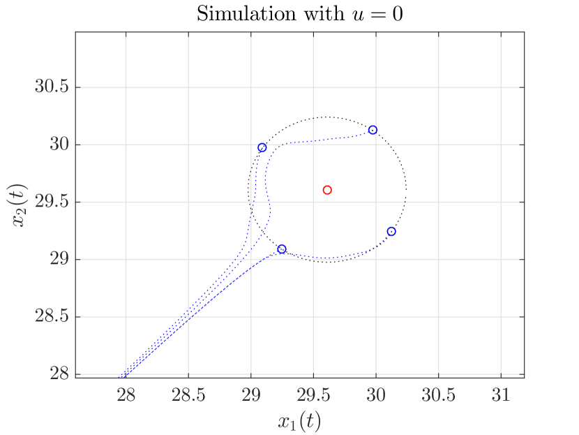
Figure 2: Simulation of the resulting interconnected system composed of (10). The circles are initial conditions. The red one is the equilibrium, i.e., the point $(x_{1},x_{2})=(r_{1},r_{1})$.

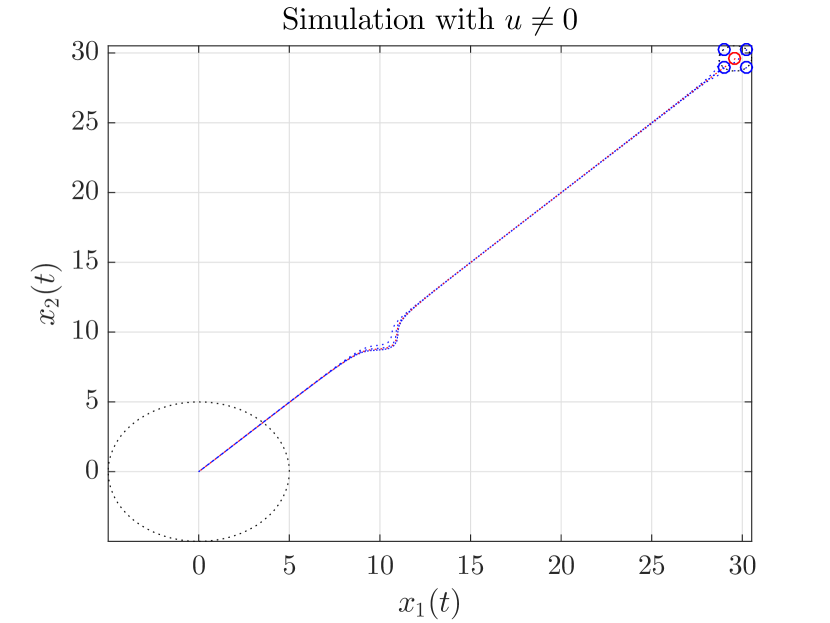
Figure 3: Simulation of the resulting interconnected system composed of (9) with $|u_{1}|_{\infty}=3$ and $|u_{2}|_{\infty}=4$. The small circles are initial conditions. The large black circumference is the set $|(x_{1},x_{2})|=5$.

III-A Proof that system (9) is ISS

To see that system (9) is ISS, for each index $i=1,2$, define for every $x_{i}\in\mathbb{R}$, the function $V_{i}(x_{i})=|x_{i}|$. The time derivative of this function along solutions to (9), for every $(x_{3-i},u_{i})\in\mathbb{R}\times\mathbb{R}$, the following inequality

$$\dot{V}_{i}(x_{i})\leq \mathtt{sign}(x_{i})\dot{x}_{i}$$

$$\leq -25g(V_{i}(x_{i}))+25h(V_{3-i}(x_{3-i}))$$

$$+\left(\tfrac{|u_{i}|_{\infty}}{a+1}\right)^{2}.$$ (11)

From here, two cases are analyzed, according to $n$ be finite or not.

Let $n$ be finite. Since the function $|g|$ positive definite, there exist functions $\alpha_{i},\alpha_{i,u}\in\mathcal{K}$ such that, for every $x_{i}\in\mathbb{R}$, the inequality

$$\dot{V}_{i}(x_{i})\leq-\alpha_{i}(V_{i}(x_{i}))+25h(V_{3-i}(x_{3-i}))+\alpha_{i,u}(|u_{i}|),$$ (12)

holds, for every $(x_{i},x_{3-i},u_{i})\in\mathbb{R}\times\mathbb{R}\times\mathbb{R}$.

Thus, system (9) is ISS. Hence, Assumption 1 holds.

III-B Proof that it satisfies small-gain conditions in the region where $g$ is not numerically constant

Assume that $n$ is finite. This implies that there exists $n+2$ regions where the function $\mathbb{R}_{\geq 0}\ni r\mapsto g(r)$ is not numerically constant. These regions are intervals $(\underline{M}_{k},\overline{M}_{k})$ of $\mathbb{R}_{\geq 0}$ where the function $g$ is strictly numerically increasing, i.e., given two values $r_{1},r_{2}\in(\underline{M}_{k},\overline{M}_{k})$ with $r_{1}<r_{2}$, $\mathbin{\mathtt{round}}(|g(r_{1})-g(r_{2}))|\neq 0$ and $g(r_{1})<g(r_{2})$. Consequently, $g$ is invertible on these intervals.

Fix $\delta\in(0,1)$ and let $|u_{i}|_{\infty}=0$. Since $\mathtt{id}<|g|$, where $\mathtt{id}$ is the identity function, together with (11), the condition

$$V_{i}(x_{i})\geq g^{-1}\left(\dfrac{h(V_{3-i}(x_{3-i}))}{1-\delta}\right)=:\gamma_{i}(V_{3-i}(x_{3-i}))$$

implies

$$\dot{V}_{i}(x_{i})\leq-\delta g(V_{i}(x_{i})).$$

Also, for every $x_{i}\in(\underline{M}_{k},\overline{M}_{k})$, the inequality

$$\gamma_{i}\circ\gamma_{3-i}(V_{i}(x_{i}))<V_{i}(x_{i})$$

When $n$ is infinite, the same analysis of item is employed. However, there are (countably many) intervals $(\underline{M}_{k},\overline{M}_{k})$. Thus, the small-gain condition holds, for the system resulting of the interconnection of (9) with $|u|_{\infty}=0$. Thus, Assumption 2 holds.

III-C Proof that it satisfies the dissipation inequality in the regions where $g$ is numerically constant

The regions where $g$ is numerically constant correspond to the closed set

$$\mathbb{R}\setminus\bigcup_{k}(\underline{M}_{k},\overline{M}_{k}).$$

For every $x_{i}$ in this set, $\mathbin{\mathtt{round}}(1-\tanh(x_{i}))=0$. Since $g$ is numerically constant, its derivative is zero. Consequently, the divergence of the vector field describing the differential equation (9) is numerically constant and equals to zero, because it is the derivative of $g$.

Consider the function

$$\begin{array}[]{rrcl}\rho:&\mathbb{R}\times\mathbb{R}&\to&\mathbb{R}_{\geq 0}\\ &(x_{1},x_{2})&\mapsto&e^{-(x_{1}+x_{2})}.\end{array}$$

Since $g$ is an odd function,

$$\mathbin{\mathtt{div}}(\rho f)(x):=\frac{\partial[\rho f_{1}]}{\partial x_{1}}(x)+\frac{\partial[\rho f_{2}]}{\partial x_{2}}(x)=\rho^{\prime}(x)\cdot f(x)$$

$$=-\mathtt{sign}(x_{1})\rho(x_{1},x_{2})\bigg{(}-\left(25+\tfrac{|u_{1}|_{\infty}}{a+1}\right)\mathtt{sign}(x_{1})|g(x_{1})|$$

$$+25h(x_{2})+\left(\tfrac{|u_{1}|_{\infty}}{a+1}\right)^{2}\bigg{)}$$

$$-\mathtt{sign}(x_{2})\rho(x_{1},x_{2})\bigg{(}-\left(25+\tfrac{|u_{2}|_{\infty}}{a+1}\right)\mathtt{sign}(x_{2})|g(x_{2})|$$

$$+25h(x_{1})+\left(\tfrac{|u_{2}|_{\infty}}{a+1}\right)^{2}\bigg{)}.$$

Assuming $n$ finite implies that, if

1. $(x_{1},x_{2})\in\mathbb{R}_{\leq 0}^{2}$, then

   $$\mathbin{\mathtt{div}}(\rho f)(x_{1},x_{2})\geq 25\rho(x_{1},x_{2})\bigg{(}|g(x_{1})|+|g(x_{2})|$$

   $$+h(x_{1})+h(x_{2})\bigg{)}$$

   $$> 0$$

2. $(x_{1},x_{2})\in\mathbb{R}_{\geq 0}^{2}$ and $|u_{1}|_{\infty}\cdot|u_{2}|_{\infty}\neq 0$, then there exists $\varepsilon>0$ such that the inequality

   $$\mathbin{\mathtt{div}}(\rho f)(x_{1},x_{2})\geq\rho(x_{1},x_{2})\bigg{(}(25+\varepsilon)|g(x_{1})|-25h(x_{1})$$

   $$-\left(\tfrac{|u_{1}|_{\infty}}{a+1}\right)^{2}+(25+\varepsilon)|g(x_{2})|-25h(x_{2})-\left(\tfrac{|u_{2}|_{\infty}}{a+1}\right)^{2}\bigg{)}$$

   holds.

   Since the function $\mathbb{R}\ni x_{i}\mapsto m_{i}(x_{i})=(25+\varepsilon)|g(x_{i})|-25h(x_{i})$ is positive definite, for each index $i=1,2$, there exists a function $\gamma^{-1}\in\mathcal{K}$ such that $\gamma^{-1}(\cdot)\leq m_{i}(\cdot)$.

   Thus, for any $\delta\in(0,1)$ the condition

   $$|x_{i}|\geq\gamma^{-1}\left(\dfrac{1}{1-\delta}\left(\frac{|u_{i}|_{\infty}}{a+1}\right)^{2}\right),i=1,2$$

   implies

   $$\mathbin{\mathtt{div}}(\rho f)(x_{1},x_{2})>0.$$

3. $x_{i}<0$ and $x_{3-i}>0$, then the situation is a combination of the two previous items.

When $n$ is infinite or $|u_{1}|_{\infty}=|u_{2}|_{\infty}=0$, the function $\mathtt{div}(\rho f)$ is positive almost for almost every $x_{i}$ in the region where $g$ is numerically constant.

Since the above inequalities are strict and hold in a closed set, there exist a suitable open set $\mathbf{D}_{k}$ and a function $q_{k}:\mathbf{D}_{k}\to\mathbb{R}_{\geq 0}$ satisfying Assumption 3.

Therefore, from Theorem 6, system resulting from the interconnection of system (9) is almost input-to-state stable.

Consider the region where $g$ is not numerically constant. In this region, there exists a subset where $\mathbin{\mathtt{div}}(\rho f)\leq 0$. To see this claim, without loss of generality let $|u_{1}|_{\infty}=|u_{2}|_{\infty}=0$, and note that $\rho(0)\mathbin{\mathtt{div}}(f)(0)=-25g^{\prime}(0)=-50\mathbin{\mathtt{sech}}^{2}(0)=-50$ and $\rho^{\prime}(0)\cdot f(0)=0$. Consequently, $\mathbin{\mathtt{div}}(\rho f)(0)=-50$. From the continuity of the functions, there exists $\varepsilon>0$ such that, for every $x_{1}$ and $x_{2}\in(-\varepsilon,\varepsilon)$, the inequality $\mathbin{\mathtt{div}}(\rho f)(x)\leq 0$ holds. Using the same reasoning, and due to the “periodicity” of the vector field $f$, the same conclusion can be obtained for every region where $g$ is not numerically constant.

IV Conclusions and discussion

In this paper, the interconnection of two ISS system for which a single small-gain condition does not hold everywhere on the positive real semi-axis has been considered.

Under the assumption that there are (infinitely many) regions where the small-gain condition hold and, outside the union of these regions, the density propagation condition holds, the trajectories of solutions to the interconnected systems that do not converge to the origin have Lebesgue measure zero. An example illustrates the proposed approach.

In a future work, the authors intend to generalize the methods for the interconnection of $n>2$ ISS systems.

References

• [1] D. Angeli “An Almost Global Notion of Input-to-State Stability” In IEEE Trans. Autom. Control 49.6, 2004, pp. 866–874 DOI: 10.1109/TAC.2004.829594
• [2] E. D. Sontag “Smooth stabilization implies coprime factorization” In IEEE Trans. Autom. Control 34.4, 1989, pp. 435–443 DOI: 10.1109/9.28018
• [3] Z.-P. Jiang, I. M. Y. Mareels and Y. Wang “A Lyapunov formulation of the nonlinear small-gain theorem for interconnected ISS systems” In Automatica 32.8, 1996, pp. 1211–1215
• [4] A. Rantzer “A dual to Lyapunov’s stability theorem” In Syst. & Contr. Lett. 42, 2001, pp. 161–168 DOI: 10.1016/S0167-6911(00)00087-6
• [5] H. Stein Shiromoto, V. Andrieu and C. Prieur “A Region-Dependent Gain Condition for Asymptotic Stability” In Automatica 52, 2015, pp. 309–316 DOI: 10.1016/j.automatica.2014.12.017
• [6] A. Isidori “Nonlinear Control Systems”, Communications and Control Engineering Springer, 1995 DOI: 10.1007/978-1-84628-615-5