Tuning-free heterogeneity pursuit in massive networks

Abstract

Heterogeneity is often natural in many contemporary applications involving massive data. While posing new challenges to effective learning, it can play a crucial role in powering meaningful scientific discoveries through the understanding of important differences among subpopulations of interest. In this paper, we exploit multiple networks with Gaussian graphs to encode the connectivity patterns of a large number of features on the subpopulations. To uncover the heterogeneity of these structures across subpopulations, we suggest a new framework of tuning-free heterogeneity pursuit (THP) via large-scale inference, where the number of networks is allowed to diverge. In particular, two new tests, the chi-based test and the linear functional-based test, are introduced and their asymptotic null distributions are established. Under mild regularity conditions, we establish that both tests are optimal in achieving the testable region boundary and the sample size requirement for the latter test is minimal. Both theoretical guarantees and the tuning-free feature stem from efficient multiple-network estimation by our newly suggested approach of heterogeneous group square-root Lasso (HGSL) for high-dimensional multi-response regression with heterogeneous noises. To solve this convex program, we further introduce a tuning-free algorithm that is scalable and enjoys provable convergence to the global optimum. Both computational and theoretical advantages of our procedure are elucidated through simulation and real data examples.

1in1in0.8in0.65in

1 Introduction

In the era of data deluge one can easily collect a massive amount of data from multiple sources, each of which may come from a certain subpopulation of a larger population of interest. For example, these subpopulations can represent different cancer types, brain disorders, or product choices. A large number of features are often associated with each subject. Understanding the heterogeneity in the association structures of these features across subpopulations can be important in empowering meaningful scientific discoveries or effective personalized choices in our lives. Meanwhile heterogeneity in the data also poses new challenges to effective learning and calls for new developments of methods, theory, and algorithms with scalability and statistical efficiency.

Heterogeneity can take different forms in various applications such as the differences among the sparsity patterns or link strengths over multiple networks, and the differences in noise levels or distributions over multiple subpopulations. To avoid potential ambiguity, we would like to make it explicit that throughout this paper, we focus only on two particular types of heterogeneity which are the heterogeneity in sparsity patterns and the heterogeneity in noise levels. To approach the problem of heterogeneous learning in these contexts, we exploit the model setting of multiple networks with Gaussian graphs each of which encodes the connectivity pattern among features for each subpopulation. The edges of these networks are characterized by the inverse covariances for each pair of nodes from a subpopulation. The focus on this particular type of network models enables us to present our main idea with technical brevity. See, for example, Teng (2016) for an account of more general network models beyond graphical models. In fact, as a popular choice of network models Gaussian graphical models involving the inverse covariances have been used widely in applications to characterize the conditional dependency structure among variables. In such models, the joint distribution of $p$ variables $X_{1},\cdots,X_{p}$ is modeled by a multivariate Gaussian distribution $N(0,\Omega^{-1})$, where the $p\times p$ matrix $\Omega$ is called the precision matrix or inverse covariance matrix of these $p$ variables. A basic fact is that each pair of variables, $X_{a}$ and $X_{b}$, are conditionally independent given all other variables if and only if the $(a,b)$th entry of the precision matrix $\Omega$ is zero. The conditional dependency structure in a Gaussian graph is therefore determined completely by the associated precision matrix $\Omega$. See, for instance, Lauritzen (1996) and Wainwright and Jordan (2008) for more detailed accounts and applications of these models.

There is a growing literature on Gaussian graphical models. Much recent attention has been given to the problem of support recovery and link strength estimation, which focuses on identifying the nonzero entries of the precision matrix and estimating their strengths. Among those endeavors, a majority of the work has focused primarily on the case of a single Gaussian graphical model; see, for example, Meinshausen and Bühlmann (2006); Yuan and Lin (2007); Friedman et al. (2008); Fan et al. (2009); Yuan (2010); Cai et al. (2011); Ravikumar et al. (2011); Liu (2013); Zhang and Zou (2014); Ren et al. (2015); Fan and Lv (2015), among many others. A common feature of this line of work is that the data is assumed to be homogeneous with all observations coming from a single population. More detailed discussions and comparisons of these methods can be found in, for instance, Ren et al. (2015) and Fan and Lv (2015). Yet as mentioned before heterogeneity in the data can be prevalent in many contemporary applications involving massive data. The existing methods for analyzing data from each individual source become insufficient due to the assumption of homogeneity. Naively combining the results from these individual analyses may also yield suboptimal performance of statistical estimation and inference.

The setting of multiple networks with Gaussian graphical models has gained more recent attention. A lot of work assumes a time-varying graphical structure across different graphs. In particular, one assumes that there is a natural ordering of the graphs and the parameters of interest vary smoothly according to this order. For these developments, some smoothing techniques such as the kernel smoothing are key to the construction of the estimators as well as the analysis of their theoretical properties. While the time-varying graphical model is not the focus of our current paper, one may refer to, for example, Zhou et al. (2010); Kolar et al. (2010); Chen et al. (2013); Qiu et al. (2016); Lu et al. (2015) for more details on this line of work.

In contrast, our setting of multiple networks with Gaussian graphical models is along another line that makes no assumption on the ordering of the graphs. In this line of work, the main assumption is a common sparsity structure across different graphs. In particular, the estimators proposed in Guo et al. (2011), Danaher et al. (2014), and Zhu et al. (2014) employ the approach of penalized likelihood with different choices of the penalty function, while the MPE method introduced in Cai et al. (2016) takes a weighted constrained $\ell_{\infty}$ and $\ell_{1}$ minimization approach, which can be seen as an extension of the CLIME estimator for a single graph (Cai et al., 2011). A common feature of such existing work is the focus on the problem of support recovery and link strength estimation. Moreover, by the nature of these methods their computational cost increases drastically with both the dimensionality and the number of graphs, which can limit their practical use in analyzing massive data sets. How to develop a scalable procedure for large-scale inference in the setting of multiple Gaussian graphical models still remains largely open.

To uncover the heterogeneity of the connectivity patterns among features across subpopulations and address the aforementioned challenges, in this paper we suggest a new framework of tuning-free heterogeneity pursuit (THP) via large-scale inference, where the number of networks is allowed to diverge and the number of features can grow exponentially with the number of observations. Distinct from the existing methods, our procedure identifies the heterogeneity in sparsity patterns among a diverging number of graphs by testing the common sparsity structure of these $k$ Gaussian graphs. Specifically, we are interested in testing the null hypothesis

$$H_{0,ab}:\ \omega_{a,b}^{0}=(\omega_{a,b}^{(1)},\cdots,\omega_{a,b}^{(k)})^{\prime}=\mathbf{0}$$ (1)

associated with the joint link strength vector for each pair of variables $1\leq a,b\leq p$ with $a\neq b$, where $\Omega^{(t)}=(\omega^{(t)}_{a,b})$ with $1\leq t\leq k$ denotes the precision matrix associated with the $t$th graph. To approach the inference problem in (1), we propose two new tests, named the chi-based test and the linear functional-based test, for two different scenarios. The former test which is for the general scenario requires no extra information from the graphs and is shown to perform well as long as the $\ell_{2}$ norm of the joint link strength vector $\omega_{a,b}^{0}$ is large. The chi-based test is named after the property that the null distribution of this test statistic is shown to converge to the chi distribution. The latter one relies on some extra information on the signs of $\omega^{(t)}_{a,b}$. Such extra information is indeed available in some applications. For example, in some genome-wide association studies (GWAS) it was discovered that the association structures can be portable between certain subpopulations (Marigorta and Navarro, 2013). In such scenario, the linear functional-based test can be constructed and shown to perform well when the $\ell_{1}$ norm of the vector $\omega_{a,b}^{0}$ becomes large.

An interesting feature of both tests is that each of them is established under mild regularity conditions to be optimal in the sense of achieving the testable region boundary, where the testable region boundary is defined as the smallest signal strength below which no test is able to detect if the observations are from the null hypothesis against the alternative hypothesis and above which some test can distinguish successfully between the two hypotheses. We further show that for the linear functional-based test, the sample size requirement is in fact minimal. A natural question is whether naively combining the tests constructed from $k$ individual graphs might suffice. Our theoretical results provide insights into this question and demonstrate the advantages of our tests in terms of weaker sample size requirement than the naive combination approach. We also would like to mention that although the main focus of our paper is on hypothesis testing, our procedure can be modified easily by introducing an additional thresholding step for support recovery; see Section 2.5 for detailed discussions and comparisons with existing approaches. In particular, our modified procedure achieves successful support recovery under milder sample size assumption than many existing methods. To the best of our knowledge, the testing of multiple networks with graphs and the optimality study are both new to the literature.

The challenges of heterogeneous learning in the setting of multiple networks are rooted on the inference with efficiency, the scalability, and the selection of tuning parameters which is often an implicit bottleneck of existing methods. Our THP framework addresses all these challenges in a harmonious fashion. Both theoretical guarantees and the tuning-free feature are enabled through efficient multiple-network estimation by our newly suggested approach of heterogeneous group square-root Lasso (HGSL) in the setting of high-dimensional multi-response regression with heterogeneous noises. More specifically, we reduce the problem of estimating $k$ graphs simultaneously to that of running $p$ multi-response regressions with heterogeneous noises. This new formulation allows us to borrow information across graphs when estimating their structures, which results in improved rates of convergence. To solve the convex programs from these multi-response regressions, we introduce a new tuning-free algorithm that is scalable and admits provable convergence to the global optimum. Compared to existing methods in the literature, our new procedure enjoys four main advantages. First, it is justified theoretically that our HGSL estimators have faster rates of convergence. Second, the HGSL method is capable of handling heterogeneous noises, the presence of which causes intrinsic difficulty for developing a tuning-free procedure. Third, our new algorithm is simple and tuning free, and scales up easily. Fourth, we provide theoretical justification on the convergence of the tuning-free algorithm.

The rest of the paper is organized as follows. Section 2 introduces the THP framework for heterogeneous learning in multiple networks via large-scale inference with the chi-based test and the linear functional-based test, and establishes their optimality properties. We present the HGSL approach along with a tuning-free algorithm for fitting high-dimensional multi-response regression with heterogeneous noises, and provide the estimation and prediction bounds for the estimator as well as a convergence analysis for the algorithm in Section 3. Section 4 details several numerical examples of simulation studies and real data analysis. We discuss some extensions of the suggested method to a few settings in Section 5. The proofs of all the results and technical details are provided in the Supplementary Material.

2 Tuning-free heterogeneity pursuit in multiple networks via large-scale inference

2.1 Model setting

As mentioned in the Introduction, we adopt the setting of multiple networks with Gaussian graphical models to encode the connectivity patterns among $p$ features $X_{1},\cdots,X_{p}$ measured on $k$ subpopulations of a general population, which yields $k$ classes of data. In this model, for each class $1\leq t\leq k$ the $p$-dimensional feature vector follows a multivariate Gaussian distribution

$$X^{(t)}=(X_{1}^{(t)},\cdots,X_{p}^{(t)})^{\prime}\sim N(0,(\Omega^{(t)})^{-1}),$$ (2)

where the superscript $(t)$ means that these $p$ features are measured on the $t$th subpopulation and $\Omega^{(t)}$ is the $p\times p$ precision matrix of the $t$th class. In addition, the distributions of $X^{(1)},\cdots,X^{(k)}$ are assumed to be independent. Each of the $k$ precision matrices $\Omega^{(t)}=(\omega_{a,b}^{(t)})_{p\times p}$ reflects the conditional dependency structure among the $p$ features $X_{1}^{(t)},\cdots,X_{p}^{(t)}$. In the high-dimensional setting where the dimensionality $p$ can be very large compared to the sample size, it is common in many applications such as genomic studies to assume that each precision matrix $\Omega^{(t)}$ has certain sparsity structure. The goals in these studies include the estimation of precision matrices $\Omega^{(t)}$ and the inference on their entries $\omega_{a,b}^{(t)}$.

When there is only one class of data, that is, $k=1$, our setting coincides with that of single Gaussian graphical model. For the general case of multiple graphs with $k\geq 2$, it can be beneficial to borrow the strength across all $k$ classes of data to achieve more accurate estimation of the $k$ precision matrices if the $k$ classes are related to each other. With this spirit, we assume that the $k$ classes share some similar sparsity structure, and the heterogeneity in sparsity patterns captures the differences among these graphical structures. In particular, we are interested in the scenario where for each pair of nodes $\left(a,b\right)$ with $1\leq a\neq b\leq p$, either $\omega_{a,b}^{(t)}=0$ simultaneously for all $1\leq t\leq k$ or alternatively the joint link strength vector $\omega_{a,b}^{0}=(\omega_{a,b}^{(1)},\cdots,\omega_{a,b}^{(k)})^{\prime}$ is significantly different from the zero vector. Throughout the paper we denote by

$$\mathcal{E}=\left\{\left(a,b\right):1\leq a\neq b\leq p\text{ and }\omega_{a,b}^{0}\neq\mathbf{0}\right\}$$ (3)

the edge set corresponding to the $k$ graphs given in model (2).

The main goal of our paper is to develop an effective and efficient procedure for testing the null hypothesis $H_{0,ab}$ defined in (1) for multiple networks, which provides an inferential approach to uncovering the heterogeneity of the feature association structures across the $k$ subpopulations. Depending on the type of the alternative hypothesis, we will introduce two different fully data-driven test statistics and establish their advantages over those obtained by naively combining the tests constructed from each individual graph.

2.2 Chi-based test

We begin with introducing the first test for our THP framework in multiple networks. To ease the presentation, we introduce some compact notation. Denote by $a_{-j}$ the subvector of a vector $a=(a_{1},\cdots,a_{p})^{\prime}$ with the $j$th component removed, and for any matrix $A=(a_{i,j})$ denote by $A_{*,j}$ its $j$th column, $A_{-j,j}$ the subvector of $A_{*,j}$ with the $j$th component removed, and $A_{*,-j}$ the submatrix of $A$ with the $j$th column removed. Our testing idea is based on a simple observation that for each $1\leq j\leq p$, the conditional distribution of $X_{j}^{(t)}$ given all remaining variables $X_{-j}^{(t)}$ in class $t$ follows the Gaussian distribution

$$X_{j}^{(t)}|X_{-j}^{(t)}\sim N(X_{-j}^{(t)\prime}C_{j}^{(t)},1/\omega_{j,j}^{(t)})$$ (4)

with the $(p-1)$-dimensional coefficient vector $C_{j}^{(t)}=-\Omega_{-j,j}^{(t)}/\omega_{j,j}^{(t)}$. Based on the distributional representation in (4), one can see that the error random variables $\epsilon_{j}^{(t)}=X_{j}^{(t)}-X_{-j}^{(t)\prime}C_{j}^{(t)}$ are independent across $t$ and follow the distribution $N(0,1/\omega^{(t)}_{j,j})$. Moreover, it holds for each pair of nodes $(a,b)$ with $1\leq a,b\leq p$ that

$$\mathrm{cov}(\epsilon_{a}^{(t)},\epsilon_{b}^{(t)})=\frac{\omega_{a,b}^{(t)}}{\omega_{a,a}^{(t)}\omega_{b,b}^{(t)}}\mbox{\rm.}$$ (5)

The key representation in (5) entails that accurate estimators of $\omega_{a,b}^{(t)}$ with $a\neq b$ can be constructed if one can estimate $\omega_{a,a}^{(t)}$, $\omega^{(t)}_{b,b}$, and $\mathrm{cov}(\epsilon_{a}^{(t)},\epsilon_{b}^{(t)})$ well.

Another important observation is that under the null hypothesis $H_{0,ab}$ in (1), the conditional distributions of the $k$ classes $X_{j}^{(t)}|X_{-j}^{(t)}$ with $1\leq t\leq k$ indeed share similar sparsity structure on the coefficient vectors $C_{j}^{(t)}$ thanks to the representation $C_{j}^{(t)}=-\Omega_{-j,j}^{(t)}/\omega_{j,j}^{(t)}$. In fact, it is clear that $C_{a,b}^{(t)}=0$ for all $1\leq t\leq k$ under $H_{0,ab}$, where $C_{a,b}^{(t)}=-\omega_{a,b}^{(t)}/\omega_{a,a}^{(t)}$ is the component of vector $C_{a}^{(t)}$ corresponding to variable $X_{b}^{(t)}$. This observation suggests that we can borrow information from different graphs when testing the joint sparsity structure of multiple graphs. Motivated by such observation, we turn the problem of multiple-network estimation into that of high-dimensional multi-response linear regression

$$\left(\begin{array}[]{c}X_{j}^{(1)}\\ X_{j}^{(2)}\\ \vdots\\ X_{j}^{(k)}\end{array}\right) = \left(\begin{array}[]{cccc}X_{-j}^{(1)}&&&\\ &X_{-j}^{(2)}&&\\ &&\ddots&\\ &&&X_{-j}^{(k)}\end{array}\right)\left(\begin{array}[]{c}C_{j}^{(1)}\\ C_{j}^{(2)}\\ \vdots\\ C_{j}^{(k)}\end{array}\right)+\left(\begin{array}[]{c}\epsilon_{j}^{(1)}\\ \epsilon_{j}^{(2)}\\ \vdots\\ \epsilon_{j}^{(k)}\end{array}\right)$$ (22)

for $1\leq j\leq p$. A distinct feature of the above multi-response regression model (22) is that it has heterogeneous noises since $\omega_{j,j}^{(t)}$ generally varies over $1\leq t\leq k$.

As mentioned before, we also have the group sparsity structure of the regression coefficient vector $C_{j}^{0}=\left(C_{j}^{(1)\prime},\cdots,C_{j}^{(k)\prime}\right)^{\prime}\in\mathbb{R}^{(p-1)k}$ in model (22). More specifically, denote the $k$-dimensional subvector of $C_{j}^{0}$ corresponding to the $l$th group by

$$C_{j(l)}^{0}=\left(C_{j,l}^{(1)},\cdots,C_{j,l}^{(k)}\right)^{\prime}.$$ (23)

Then we see that $C_{j(l)}^{0}=\bf{0}$ for all pairs $(j,l)\in\mathcal{E}^{c}$, the complement of $\mathcal{E}$ defined in (3). We will suggest in Section 3 an efficient estimation procedure that utilizes the group sparsity structure in the regression coefficients and also accounts for the heterogeneity in the noises in model (22).

From now on we work with a sample from model (2) that is comprised of $n^{(t)}$ independent and identically distributed (i.i.d.) observations $X_{1,\ast}^{(t)},\cdots,X_{n^{(t)},\ast}^{(t)}$ for each class $1\leq t\leq k$, where $X_{i,\ast}^{(t)}=(X_{i,1}^{(t)},\cdots,X_{i,p}^{(t)})^{\prime}\sim N(0,(\Omega^{(t)})^{-1})$ and the observations across different classes are independent. Suppose that we have some initial estimator $\hat{C}_{j}^{0}=(\hat{C}_{j}^{(1)\prime},\cdots,\hat{C}_{j}^{(k)\prime})^{\prime}$ for the $(p-1)k$-dimensional regression coefficient vector $C_{j}^{0}$, whose construction is detailed in Section 3. Then the random errors for each $1\leq t\leq k$ can be estimated by the residuals

$$\hat{E}_{i,j}^{(t)}=X_{i,j}^{(t)}-X_{i,-j}^{(t)\prime}\hat{C}_{j}^{(t)}$$ (24)

with $\ 1\leq i\leq n^{(t)}$ and $1\leq j\leq p$. In view of the representation in (5), we can estimate $\omega_{j,j}^{(t)}$ associated with the noise level of class $t$ as $\hat{\omega}_{j,j}^{(t)}=n^{(t)}/(\sum_{i=1}^{n^{(t)}}\hat{E}_{i,j}^{(t)}\hat{E}_{i,j}^{(t)})$. In contrast, the estimation of $\omega^{(t)}_{a,b}$ with $a\neq b$ is slightly more complicated. To estimate the negative covariance $-\mathrm{cov}(\epsilon_{a}^{(t)},\epsilon_{b}^{(t)})=-\omega_{a,b}^{(t)}/(\omega_{a,a}^{(t)}\omega_{b,b}^{(t)})$, we exploit the following bias corrected statistic

$$T_{n,k,a,b}^{(t)}=\frac{1}{n^{(t)}}\left[\sum_{i=1}^{n^{(t)}}\hat{E}_{i,a}^{(t)}\hat{E}_{i,b}^{(t)}+\sum_{i=1}^{n^{(t)}}\left(\hat{E}_{i,a}^{(t)}\right)^{2}\hat{C}_{b,a}^{(t)}+\sum_{i=1}^{n^{(t)}}\left(\hat{E}_{i,b}^{(t)}\right)^{2}\hat{C}_{a,b}^{(t)}\right].$$ (25)

Observe that the first term on the right-hand side of (25) corresponds to the sample covariance of the residuals from variables $X_{a}^{(t)}$ and $X_{b}^{(t)}$. When $a=b$, this sample covariance is asymptotically unbiased in estimating $\mathrm{var}(\epsilon_{a}^{(t)})=1/\omega_{a,a}^{(t)}$. Such sample covariance is, however, biased in the case of $a\neq b$ and thus two additional terms are introduced for $T_{n,k,a,b}^{(t)}$ in (25) to correct the bias. Indeed, we can show that after the bias correction the statistic $T_{n,k,a,b}^{(t)}$ is asymptotically close to the statistic

$$J_{n,k,a,b}^{(t)}=\left[1-\omega_{a,a}^{(t)}(\hat{\omega}_{a,a}^{(t)})^{-1}-\omega_{b,b}^{(t)}(\hat{\omega}_{b,b}^{(t)})^{-1}\right]\frac{\omega_{a,b}^{(t)}}{\omega_{a,a}^{(t)}\omega_{b,b}^{(t)}},$$ (26)

which is in turn asymptotically close to the negative covariance $-\mathrm{cov}(\epsilon_{a}^{(t)},\epsilon_{b}^{(t)})$.

When there is only a single graph, that is, $k=1$, the above statistic $T^{(t)}_{n,k,a,b}$ in (25) reduces to the one introduced in Liu (2013) to address the bias issue in the testing for a single Gaussian graph. In the scenario of multiple graphs, we observe a similar phenomenon and provide in Theorem 1 later a formal theoretical justification. It is worth mentioning that the key estimators $\hat{\omega}_{j,j}^{(t)}$ and $T_{n,k,a,b}^{(t)}$ introduced above are constructed using the residuals $\hat{E}_{i,j}^{(t)}$ instead of the estimated regression coefficients $\hat{C}_{a,b}^{(t)}$, though the regression coefficients $C_{a,b}^{(t)}$ are also closely related to the entries of the precision matrix $\Omega^{(t)}$. The main advantage of using residuals $\hat{E}_{i,j}^{(t)}$ over coefficients $\hat{C}_{a,b}^{(t)}$ is rooted on the fact that obtaining asymptotically unbiased estimates of the latter is much more challenging in high dimensions, largely due to the well-known bias issue associated with the regularization methods, than accurately estimating the former, which is closely related to the prediction problem.

The new formulation in (22) not only allows us to solve the problem of multiple-graph estimation efficiently through $p$ multi-response regressions as detailed in Section 3, but also enables us to construct new tests that are more powerful than existing methods by borrowing information from different graphs. We are now ready to present the first such test. Due to the group sparsity structure and the target of our null hypothesis $H_{0,ab}:\omega_{a,b}^{0}=\mathbf{0}$ in (1), we naturally construct our test statistics using certain functions of all statistics $T_{n,k,a,b}^{(t)}$ in (25) with $1\leq t\leq k$. Thanks to the joint estimation accuracy for the $(p-1)k$-dimensional regression coefficient vector $C_{j}^{0}$, we define our first test statistic, the chi-based test statistic $U_{n,k,a,b}$, as

$$U_{n,k,a,b}^{2}=\sum_{t=1}^{k}n^{(t)}\hat{\omega}_{b,b}^{(t)}\hat{\omega}_{a,a}^{(t)}\left(T_{n,k,a,b}^{(t)}\right)^{2}$$ (27)

for testing the null hypothesis $H_{0,ab}$ against the alternative hypothesis for which the condition is imposed on the $\ell_{2}$ norm $\|\omega_{a,b}^{0}\|$. In other words, our test statistic is powerful whenever the signal strength $\|\omega_{a,b}^{0}\|$ is larger than some testable region boundary, which will be characterized later in Section 2.4.

To characterize the limiting distribution of the chi-based test statistic $U_{n,k,a,b}$ in (27) under the null, we introduce two additional statistics $V_{n,k,a,b}^{\ast(t)}$ and $U_{n,k,a,b}^{\ast}$ as

$$V_{n,k,a,b}^{\ast(t)} = \mathchoice{{\hbox{$\displaystyle\sqrt{\frac{\omega_{b,b}^{(t)}\tilde{\omega}_{a,a}^{(t)}}{n^{(t)}}\,}$}\lower 0.4pt\hbox{\vrule height=15.55833pt,depth=-12.44672pt}}}{{\hbox{$\textstyle\sqrt{\frac{\omega_{b,b}^{(t)}\tilde{\omega}_{a,a}^{(t)}}{n^{(t)}}\,}$}\lower 0.4pt\hbox{\vrule height=13.14583pt,depth=-10.51671pt}}}{{\hbox{$\scriptstyle\sqrt{\frac{\omega_{b,b}^{(t)}\tilde{\omega}_{a,a}^{(t)}}{n^{(t)}}\,}$}\lower 0.4pt\hbox{\vrule height=12.71527pt,depth=-10.17226pt}}}{{\hbox{$\scriptscriptstyle\sqrt{\frac{\omega_{b,b}^{(t)}\tilde{\omega}_{a,a}^{(t)}}{n^{(t)}}\,}$}\lower 0.4pt\hbox{\vrule height=12.71527pt,depth=-10.17226pt}}}\sum_{i=1}^{n^{(t)}}\left(E_{i,a}^{(t)}E_{i,b}^{(t)}-\mathbb{E}E_{i,a}^{(t)}E_{i,b}^{(t)}\right),$$ (28)

$$U_{n,k,a,b}^{\ast 2} = \sum_{t=1}^{k}\left(V_{n,k,a,b}^{\ast(t)}\right)^{2}=\sum_{t=1}^{k}\frac{\omega_{b,b}^{(t)}\tilde{\omega}_{a,a}^{(t)}}{n^{(t)}}\left[\sum_{i=1}^{n^{(t)}}\left(E_{i,a}^{(t)}E_{i,b}^{(t)}-\mathbb{E}E_{i,a}^{(t)}E_{i,b}^{(t)}\right)\right]^{2},$$ (29)

where $E^{(t)}_{i,j}=X_{i,j}^{(t)}-X_{i,-j}^{(t)\prime}C_{j}^{(t)}$ is the random error and $\tilde{\omega}_{j,j}^{(t)}=n^{(t)}/(E_{*,j}^{(t)\prime}E_{*,j}^{(t)})$ is the oracle estimator of $\omega_{jj}^{(t)}$ since the random error vector $E_{\ast,j}^{(t)}=(E_{1,j}^{(t)},\cdots,E_{n^{(t)},j}^{(t)})^{\prime}$ is unobservable in practice. It is interesting to observe that under the null, the Gaussian vector $E_{\ast,b}^{(t)}\sim N(0,(\omega_{b,b}^{(t)})^{-1}I)$ is independent of $E_{\ast,a}^{(t)}$, which entails that $V_{n,k,a,b}^{\ast(t)}\sim N(0,1)$ and they are independent of each other over $1\leq t\leq k$. Consequently, under the null hypothesis $H_{0,ab}$ in (1) it holds that $U_{n,k,a,b}^{\ast 2}\sim\chi^{2}(k)$.

Before formally presenting our first main result, we introduce the following two regularity conditions on our model (2).

Condition 1

There exists some constant $M>0$ such that $1/M\leq\lambda_{\min}(\Omega^{(t)})\leq\lambda_{\max}(\Omega^{(t)})\leq M$ for each $1\leq t\leq k$, where $\lambda_{\min}$ and $\lambda_{\max}$ denote the smallest and largest eigenvalues of a matrix.

Condition 2

It holds that $n^{(1)}\asymp\cdots\asymp n^{(k)}$ with $\max_{1\leq t\leq k}\{n^{(t)}\}/n^{(0)}\leq M_{0}$, where $\asymp$ means the same order, $n^{(0)}=\min_{1\leq t\leq k}\{n^{(t)}\}$, and $M_{0}$ is some positive constant.

The well-conditionedness of the precision matrices $\Omega^{(t)}$ assumed in Condition 1 simplifies our technical presentation. For simplicity, we also assume in Condition 2 that our sample is balanced with the sample sizes of each of the $k$ classes comparable to each other. With slight abuse of notation, we denote by $n^{(0)}$ this common level whenever the rate is involved. We proceed with introducing additional notation and technical conditions. Denote by $\Delta_{j}=\hat{C}_{j}^{0}-C_{j}^{0}$ and $\Delta_{j(l)}=\hat{C}_{j(l)}^{0}-C_{j(l)}^{0}$ the estimation errors of $\hat{C}_{j}^{0}$ and $\hat{C}_{j(l)}^{0}$, respectively, with the $k$-dimensional subvector $\hat{C}_{j(l)}^{0}$ defined in a similar way to $C_{j(l)}^{0}$ in (23). To characterize the sparsity level, we define the joint sparsity of the $k$ networks as the maximum node degree corresponding to the edge set $\mathcal{E}$ in (3),

$$s\equiv\max_{1\leq a\leq p}\sum_{1\leq b\neq a\leq p}1\{\omega_{a,b}^{0}\neq\mathbf{0}\}.$$ (30)

We further assume that with high probability the initial estimator $\hat{C}_{j}^{0}$ satisfies

$$\frac{1}{\mathchoice{{\hbox{$\displaystyle\sqrt{k\,}$}\lower 0.4pt\hbox{\vrule height=6.94444pt,depth=-5.55559pt}}}{{\hbox{$\textstyle\sqrt{k\,}$}\lower 0.4pt\hbox{\vrule height=6.94444pt,depth=-5.55559pt}}}{{\hbox{$\scriptstyle\sqrt{k\,}$}\lower 0.4pt\hbox{\vrule height=4.8611pt,depth=-3.8889pt}}}{{\hbox{$\scriptscriptstyle\sqrt{k\,}$}\lower 0.4pt\hbox{\vrule height=3.47221pt,depth=-2.77779pt}}}}\left\|\Delta_{j}\right\| \leq C_{1}\left[s\frac{1+(\log p)/k}{n^{(0)}}\right]^{1/2},$$ (31)

$$\sum_{l\neq j}\frac{1}{\mathchoice{{\hbox{$\displaystyle\sqrt{k\,}$}\lower 0.4pt\hbox{\vrule height=6.94444pt,depth=-5.55559pt}}}{{\hbox{$\textstyle\sqrt{k\,}$}\lower 0.4pt\hbox{\vrule height=6.94444pt,depth=-5.55559pt}}}{{\hbox{$\scriptstyle\sqrt{k\,}$}\lower 0.4pt\hbox{\vrule height=4.8611pt,depth=-3.8889pt}}}{{\hbox{$\scriptscriptstyle\sqrt{k\,}$}\lower 0.4pt\hbox{\vrule height=3.47221pt,depth=-2.77779pt}}}}\left\|\Delta_{j(l)}\right\| \leq C_{2}s\left[\frac{1+(\log p)/k}{n^{(0)}}\right]^{1/2},$$ (32)

$$\frac{1}{k}\sum_{t=1}^{k}\frac{\left\|X_{\ast,-j}^{(t)}\left(\hat{C}_{j}^{(t)}-C_{j}^{(t)}\right)\right\|^{2}}{n^{(t)}} \leq C_{3}s\frac{1+(\log p)/k}{n^{(0)}},$$ (33)

where $C_{1},C_{2}$, and $C_{3}$ are some positive constants and $\|\cdot\|$ denotes the $\ell_{2}$ norm. The properties (31)–(33) are crucial working assumptions in our testing for $k$ networks.

Indeed, the new tuning-free approach of HGSL suggested in Section 3 guarantees that we can obtain initial estimators $\hat{C}_{j}^{0}$ each satisfying all these properties (31)–(33) with probability at least $1-C_{0}p^{1-\delta}$ for some positive constants $C_{0}$ and $\delta>1$. A distinct feature is that the analysis of our tuning-free estimator is new due to the heterogeneity of noises across different classes, which makes typical tuning-free procedures such as the scaled Lasso (Sun and Zhang, 2012) and the square-root Lasso (Belloni et al., 2011) no longer work in the current setting; see Section 3 for more detailed discussions.

Theorem 1

Assume that Conditions 1–2 hold, the initial estimators $\hat{C}_{j}^{0}$ each satisfy properties (31)–(33) with probability at least $1-C_{0}p^{1-\delta}$, $s\left(k+\log p\right)/n^{(0)}=o(1)$, and $\log(k/\delta_{1})=O\{s[1+(\log p)/k]\}$ for some constants $C_{0}>0,\delta>1$ and $\delta_{1}=o(1)$. Then for each pair $(a,b)$ with $1\leq a\neq b\leq p$, it holds with probability at least $1-(12+C_{0})p^{1-\delta}-4\delta_{1}$ that

$$\left|\left[\sum_{t=1}^{k}n^{(t)}\hat{\omega}_{b,b}^{(t)}\hat{\omega}_{a,a}^{(t)}\left(T_{n,k,a,b}^{(t)}-J_{n,k,a,b}^{(t)}\right)^{2}\right]^{1/2}-U_{n,k,a,b}^{\ast}\right| \leq C\left(s\frac{k+\log p}{\mathchoice{{\hbox{$\displaystyle\sqrt{n^{(0)}\,}$}\lower 0.4pt\hbox{\vrule height=6.40555pt,depth=-5.12447pt}}}{{\hbox{$\textstyle\sqrt{n^{(0)}\,}$}\lower 0.4pt\hbox{\vrule height=6.40555pt,depth=-5.12447pt}}}{{\hbox{$\scriptstyle\sqrt{n^{(0)}\,}$}\lower 0.4pt\hbox{\vrule height=4.51389pt,depth=-3.61113pt}}}{{\hbox{$\scriptscriptstyle\sqrt{n^{(0)}\,}$}\lower 0.4pt\hbox{\vrule height=3.65277pt,depth=-2.92224pt}}}}\right),$$

where $C>0$ is some constant. Moreover, under null hypothesis $H_{0,ab}$ in (1) we have $U_{n,k,a,b}^{\ast 2}\sim\chi^{2}(k)$ and with the same probability bound that $\left|U_{n,k,a,b}-U_{n,k,a,b}^{\ast}\right|\leq C\left(s\frac{k+\log p}{\mathchoice{{\hbox{$\displaystyle\sqrt{n^{(0)}\,}$}\lower 0.4pt\hbox{\vrule height=4.48389pt,depth=-3.58713pt}}}{{\hbox{$\textstyle\sqrt{n^{(0)}\,}$}\lower 0.4pt\hbox{\vrule height=4.48389pt,depth=-3.58713pt}}}{{\hbox{$\scriptstyle\sqrt{n^{(0)}\,}$}\lower 0.4pt\hbox{\vrule height=3.15971pt,depth=-2.52779pt}}}{{\hbox{$\scriptscriptstyle\sqrt{n^{(0)}\,}$}\lower 0.4pt\hbox{\vrule height=2.55695pt,depth=-2.04558pt}}}}\right).$

The coupling result in Theorem 1 motivates us to propose the chi-based test $\phi_{2}$ defined as

$$\phi_{2}=1\left\{U_{n,k,a,b}>z_{k}^{l2}(1-\alpha)\right\}$$ (34)

for our THP framework in multiple networks which tests the null hypothesis $H_{0,ab}$ in (1) using the test statistic $U_{n,k,a,b}$ given in (27), where $\alpha\in\left(0,1\right)$ is a fixed significance level and $z_{k}^{l2}(1-\alpha)$ denotes the $100(1-\alpha)$th percentile of the chi distribution with degrees of freedom $k$. The name of this test is from the property that the null distribution of the test statistic is asymptotically close to the chi distribution.

Proposition 1

Assume that all the conditions of Theorem 1 hold and $s^{2}(k+\log p)^{2}=o(n^{(0)})$. Then the chi-based test $\phi_{2}$ in (34) has asymptotic significance level $\alpha$.

As formally justified in Proposition 1, the chi-based test $\phi_{2}$ introduced in (34) is indeed an asymptotic test with significance level $\alpha$ under the sample size requirement of $n^{(0)}\gg s^{2}(k+\log p)^{2}$, in the asymptotic setting in which the number of nodes $p$, the number of networks $k$, and the joint sparsity of the networks $s$ can diverge simultaneously as the common level of sample sizes $n^{(0)}\rightarrow\infty$.

2.3 Linear functional-based test

The chi-based test $\phi_{2}$ introduced in Section 2.2 serves as a general procedure to test whether the joint link strength vector $\omega_{a,b}^{0}$ is zero when there is no additional information assumed on the $k$ networks. In some scenarios when certain extra knowledge is available, it is possible to design more powerful testing procedures. In this spirit, we now present an alternative test for our THP framework in multiple networks based on a linear functional of $\omega_{a,b}^{0}$, which is closely related to its $\ell_{1}$ norm. The main motivation is that in some applications such as the GWAS example mentioned in the Introduction (Marigorta and Navarro, 2013), the sign relationship of some target edge across $k$ graphs is provided implicitly or explicitly. For example, one may expect that all the $\omega_{a,b}^{(t)}$ with $1\leq t\leq k$ share the same sign, that is, they are either all nonpositive or all nonnegative. In such scenario, testing the null hypothesis $H_{0,ab}:\omega_{a,b}^{0}=\mathbf{0}$ is equivalent to testing $\|\omega_{a,b}^{0}\|_{1}=|\sum_{t=1}^{k}\omega_{a,b}^{(t)}|=0$. In a more general setting, the sign relationship can be represented by a unique sign vector $\xi=(\xi_{1},\cdots,\xi_{k})^{\prime}\in\{1,-1\}^{k}$, up to a single sign, such that $\|\omega_{a,b}^{0}\|_{1}=\sum_{t=1}^{k}\xi_{t}\omega_{a,b}^{(t)}$ or $\|\omega_{a,b}^{0}\|_{1}=|\sum_{t=1}^{k}\xi_{t}\omega_{a,b}^{(t)}|$, and thus the null hypothesis $H_{0,ab}:\omega_{a,b}^{0}=\mathbf{0}$ takes an equivalent form of $\|\omega_{a,b}^{0}\|_{1}=|\sum_{t=1}^{k}\xi_{t}\omega_{a,b}^{(t)}|=0$.

Given the above sign vector $\xi$, we define our second test statistic, the linear functional-based test statistic $V_{n,k,a,b}(\xi)$, as

$$V_{n,k,a,b}(\xi)=\sum_{t=1}^{k}\xi_{t}\mathchoice{{\hbox{$\displaystyle\sqrt{n^{(t)}\hat{\omega}_{a,a}^{(t)}\hat{\omega}_{b,b}^{(t)}\,}$}\lower 0.4pt\hbox{\vrule height=9.32224pt,depth=-7.45782pt}}}{{\hbox{$\textstyle\sqrt{n^{(t)}\hat{\omega}_{a,a}^{(t)}\hat{\omega}_{b,b}^{(t)}\,}$}\lower 0.4pt\hbox{\vrule height=9.32224pt,depth=-7.45782pt}}}{{\hbox{$\scriptstyle\sqrt{n^{(t)}\hat{\omega}_{a,a}^{(t)}\hat{\omega}_{b,b}^{(t)}\,}$}\lower 0.4pt\hbox{\vrule height=8.72223pt,depth=-6.97781pt}}}{{\hbox{$\scriptscriptstyle\sqrt{n^{(t)}\hat{\omega}_{a,a}^{(t)}\hat{\omega}_{b,b}^{(t)}\,}$}\lower 0.4pt\hbox{\vrule height=8.72223pt,depth=-6.97781pt}}}T_{n,k,a,b}^{(t)}$$ (35)

with the bias corrected statistic $T_{n,k,a,b}^{(t)}$ given in (25). To characterize the limiting distribution of the linear functional-based test statistic $V_{n,k,a,b}$ under the null, we introduce another statistic $V_{n,k,a,b}^{\ast}(\xi)$ as

$$V_{n,k,a,b}^{\ast}(\xi)=\sum_{t=1}^{k}\xi_{t}V_{n,k,a,b}^{\ast(t)}=\sum_{t=1}^{k}\xi_{t}\mathchoice{{\hbox{$\displaystyle\sqrt{\frac{\omega_{b,b}^{(t)}\tilde{\omega}_{a,a}^{(t)}}{n^{(t)}}\,}$}\lower 0.4pt\hbox{\vrule height=15.55833pt,depth=-12.44672pt}}}{{\hbox{$\textstyle\sqrt{\frac{\omega_{b,b}^{(t)}\tilde{\omega}_{a,a}^{(t)}}{n^{(t)}}\,}$}\lower 0.4pt\hbox{\vrule height=13.14583pt,depth=-10.51671pt}}}{{\hbox{$\scriptstyle\sqrt{\frac{\omega_{b,b}^{(t)}\tilde{\omega}_{a,a}^{(t)}}{n^{(t)}}\,}$}\lower 0.4pt\hbox{\vrule height=12.71527pt,depth=-10.17226pt}}}{{\hbox{$\scriptscriptstyle\sqrt{\frac{\omega_{b,b}^{(t)}\tilde{\omega}_{a,a}^{(t)}}{n^{(t)}}\,}$}\lower 0.4pt\hbox{\vrule height=12.71527pt,depth=-10.17226pt}}}\sum_{i=1}^{n^{(t)}}\left(E_{i,a}^{(t)}E_{i,b}^{(t)}-\mathbb{E}E_{i,a}^{(t)}E_{i,b}^{(t)}\right),$$

where the statistic $V_{n,k,a,b}^{\ast(t)}$ is given in (28). With the extra sign information, our new test statistic is powerful whenever the signal strength $\|\omega_{a,b}^{0}\|_{1}$ becomes large; see Section 2.4 for the characterization of the testable region boundary under the alternative hypothesis for which the condition is imposed on the $\ell_{1}$ norm $\|\omega_{a,b}^{0}\|_{1}$. It is easy to see that under the null, $V_{n,k,a,b}^{\ast(t)}\sim N(0,1)$ are independent of each other over $1\leq t\leq k$, and consequently $V_{n,k,a,b}^{\ast}(\xi)\sim N(0,k)$ for any given sign vector $\xi$.

Theorem 2

Assume that all the conditions of Theorem 1 hold. Then for each pair $(a,b)$ with $1\leq a\neq b\leq p$, it holds with probability at least $1-(12+C_{0})p^{1-\delta}-4\delta_{1}$ that

$$\left|\sum_{t=1}^{k}\xi_{t}\left[\mathchoice{{\hbox{$\displaystyle\sqrt{n^{(t)}\hat{\omega}_{b,b}^{(t)}\hat{\omega}_{a,a}^{(t)}\,}$}\lower 0.4pt\hbox{\vrule height=9.32224pt,depth=-7.45782pt}}}{{\hbox{$\textstyle\sqrt{n^{(t)}\hat{\omega}_{b,b}^{(t)}\hat{\omega}_{a,a}^{(t)}\,}$}\lower 0.4pt\hbox{\vrule height=9.32224pt,depth=-7.45782pt}}}{{\hbox{$\scriptstyle\sqrt{n^{(t)}\hat{\omega}_{b,b}^{(t)}\hat{\omega}_{a,a}^{(t)}\,}$}\lower 0.4pt\hbox{\vrule height=8.72223pt,depth=-6.97781pt}}}{{\hbox{$\scriptscriptstyle\sqrt{n^{(t)}\hat{\omega}_{b,b}^{(t)}\hat{\omega}_{a,a}^{(t)}\,}$}\lower 0.4pt\hbox{\vrule height=8.72223pt,depth=-6.97781pt}}}\left(T_{n,k,a,b}^{(t)}-J_{n,k,a,b}^{(t)}\right)-V_{n,k,a,b}^{\ast(t)}\right]\right| \leq C\left(s\frac{k+\log p}{\mathchoice{{\hbox{$\displaystyle\sqrt{n^{(0)}\,}$}\lower 0.4pt\hbox{\vrule height=6.40555pt,depth=-5.12447pt}}}{{\hbox{$\textstyle\sqrt{n^{(0)}\,}$}\lower 0.4pt\hbox{\vrule height=6.40555pt,depth=-5.12447pt}}}{{\hbox{$\scriptstyle\sqrt{n^{(0)}\,}$}\lower 0.4pt\hbox{\vrule height=4.51389pt,depth=-3.61113pt}}}{{\hbox{$\scriptscriptstyle\sqrt{n^{(0)}\,}$}\lower 0.4pt\hbox{\vrule height=3.65277pt,depth=-2.92224pt}}}}\right),$$ (36)

where $C>0$ is some constant. Moreover, under null hypothesis $H_{0,ab}$ in (1) we have $J_{n,k,a,b}^{(t)}=0$, $V_{n,k,a,b}^{\ast}(\xi)\sim N(0,k)$ and with the same probability bound, $\left|V_{n,k,a,b}(\xi)-V_{n,k,a,b}^{\ast}(\xi)\right|\leq C\left(s\frac{k+\log p}{\mathchoice{{\hbox{$\displaystyle\sqrt{n^{(0)}\,}$}\lower 0.4pt\hbox{\vrule height=4.48389pt,depth=-3.58713pt}}}{{\hbox{$\textstyle\sqrt{n^{(0)}\,}$}\lower 0.4pt\hbox{\vrule height=4.48389pt,depth=-3.58713pt}}}{{\hbox{$\scriptstyle\sqrt{n^{(0)}\,}$}\lower 0.4pt\hbox{\vrule height=3.15971pt,depth=-2.52779pt}}}{{\hbox{$\scriptscriptstyle\sqrt{n^{(0)}\,}$}\lower 0.4pt\hbox{\vrule height=2.55695pt,depth=-2.04558pt}}}}\right).$

Theorem 2 quantifies the asymptotic behavior of the linear functional-based test statistic $V_{n,k,a,b}(\xi)$ under the null hypothesis $H_{0,ab}$ in (1). Assume further that the sign vector $\xi$ is given uniquely such that $\|\omega_{a,b}^{0}\|_{1}=\sum_{t=1}^{k}\xi_{t}\omega_{a,b}^{(t)}$ under the alternative hypothesis. Then Theorem 2 and the definition of the statistic $J_{n,k,a,b}^{(t)}$ in (26) motivate us to propose a one-sided test, the linear functional-based test $\phi_{1}$, defined as

$$\phi_{1}=1\left\{\frac{V_{n,k,a,b}(\xi)}{\mathchoice{{\hbox{$\displaystyle\sqrt{k\,}$}\lower 0.4pt\hbox{\vrule height=6.94444pt,depth=-5.55559pt}}}{{\hbox{$\textstyle\sqrt{k\,}$}\lower 0.4pt\hbox{\vrule height=6.94444pt,depth=-5.55559pt}}}{{\hbox{$\scriptstyle\sqrt{k\,}$}\lower 0.4pt\hbox{\vrule height=4.8611pt,depth=-3.8889pt}}}{{\hbox{$\scriptscriptstyle\sqrt{k\,}$}\lower 0.4pt\hbox{\vrule height=3.47221pt,depth=-2.77779pt}}}}<z(\alpha)\right\}$$ (37)

for our THP framework in multiple networks, where $\alpha\in\left(0,1\right)$ is a fixed significance level and $z(\alpha)$ stands for the $100\alpha$th percentile of the standard Gaussian distribution. When the sign vector $\xi$ is given up to a single sign, for example, when we know only that all the signs $\xi_{t}$ with $1\leq t\leq k$ are identical, it is more natural to define a two-sided test. We omit the details of such two-sided test for simplicity.

Proposition 2

Assume that all the conditions of Theorem 2 hold and $s^{2}k^{-1}(k+\log p)^{2}=o(n^{(0)})$. Then the linear functional-based test $\phi_{1}$ in (37) has asymptotic significance level $\alpha$.

Proposition 2 which is based on Theorem 2 shows that the linear functional-based test $\phi_{1}$ introduced in (37) is indeed an asymptotic test with significance level $\alpha$ under the sample size requirement of $n^{(0)}\gg s^{2}k^{-1}(k+\log p)^{2}$. It is worth mentioning that most existing results in the literature either focus on testing procedures for a single graph or develop estimation procedures for multiple graphs without statistical inference in high dimensions. In contrast, our developments in Theorems 1–2 and Propositions 1–2 provide procedures of large-scale inference in multiple graphs for the first time. For the case of a single graph with $k=1$, our test statistics essentially reduce to the one introduced in Liu (2013). This suggests an alternative way of constructing test statistics, which is to construct a test statistic for each individual graph $1\leq t\leq k$ as in Liu (2013) and then naively pool them together in the same way as for our tests $\phi_{2}$ and $\phi_{1}$.

Let us gain some insights into our tests with a comparison to the above naive combination procedure. The advantage of our linear functional-based test $\phi_{1}$ is reflected on the sample size requirement of $s^{2}k^{-1}(k+\log p)^{2}=o(n^{(0)})$ established in Proposition 2, thanks to the information of structural similarity across the $k$ graphs which makes the working assumptions (31)–(33) possible. In comparison, to test the null hypothesis $H_{0,ab}:\omega_{a,b}^{0}=\mathbf{0}$ one can also apply the procedure in Liu (2013) to each of the $k$ graphs and then construct a similar linear functional-based test as in (37). For such naive combination procedure, it can be shown that a stronger sample size assumption $s^{2}k\left(\log p\right)^{2}=o(n^{(0)})$ is required. In fact, we further establish in Section 2.4 that the sample size requirement $s^{2}k^{-1}(k+\log p)^{2}=o(n^{(0)})$ for our linear functional-based test $\phi_{1}$ is minimal in a decision theoretic framework.

Similarly the advantage of our chi-based test $\phi_{2}$ is rooted on the sample size requirement of $s^{2}(k+\log p)^{2}=o(n^{(0)})$ obtained in Proposition 1. In contrast, one can also construct a similar chi-based test as in (34) based on the residuals $\hat{E}_{i,j}^{(t)}$ which are obtained through an application of the procedure in Liu (2013) to each individual graph. For such naive combination testing procedure, it can be shown that the sample size assumption $s^{2}k\left(\log p\right)^{2}=o(n^{(0)})$ is required. This demonstrates that in a range of typical scenarios when the number of networks does not grow excessively fast with $k=o\{\left(\log p\right)^{2}\}$, our chi-based test $\phi_{2}$ indeed has a weaker sample size requirement.

2.4 Optimality of tests and minimum sample size requirement

So far we have introduced our THP framework in multiple networks with two different types of tests for testing the null hypothesis $H_{0,ab}:\omega_{a,b}^{0}=\mathbf{0}$ in (1). The constructions of our test statistics are motivated by the possible alternative hypothesis. In particular, the chi-based test $\phi_{2}$ should be powerful as long as the joint link strength $\|\omega_{a,b}^{0}\|$ is away from zero, while the linear functional-based test $\phi_{1}$ will be powerful when the signs of $\omega_{a,b}^{0}$ are known and $\|\omega_{a,b}^{0}\|_{1}$ becomes large. Along this direction, we now further investigate two types of composite alternative hypotheses. We define the set of all $s$-sparse multiple networks as

$$\mathcal{F}(s)=\mathcal{F}(s,M)=\left\{\Omega^{0}:\max_{1\leq a\leq p}\sum_{1\leq b\neq a\leq p}1\{\omega_{a,b}^{0}\neq\mathbf{0}\}\leq s\mbox{ and Condition \ref{CondA1} holds}\right\},$$ (38)

where $\Omega^{0}=\{\Omega^{(t)}\}_{t=1}^{k}$ stands for the set of $k$ precision matrices with slight abuse of notation and $s$ is some positive integer. Then the null hypothesis $H_{0,ab}$ in (1) can be rewritten as

$$H_{0,ab}=H_{0,ab}(s):\Omega^{0}\in\mathcal{N}(s)\equiv\left\{\Omega^{0}:\Omega^{0}\in\mathcal{F}(s),\,\omega_{a,b}^{0}=\mathbf{0}\right\}.$$ (39)

In particular, we consider the following two alternative hypotheses

$$H_{1,ab}^{l2}(s,\epsilon) : \Omega^{0}\in\mathcal{A}^{l2}(s,\epsilon)\equiv\left\{\Omega^{0}:\Omega^{0}\in\mathcal{F}(s),\,\left\|\omega_{a,b}^{0}\right\|\geq\epsilon\right\},$$ (40)

$$H_{1,ab}^{l1}(s,\epsilon,\xi) : \Omega^{0}\in\mathcal{A}^{l1}(s,\epsilon,\xi)\equiv\left\{\Omega^{0}:\Omega^{0}\in\mathcal{F}(s),\,\xi^{\prime}\omega_{a,b}^{0}=\left\|\omega_{a,b}^{0}\right\|_{1}\geq\epsilon\right\},$$ (41)

where the former is introduced to investigate the chi-based test $\phi_{2}$, the latter is for the linear functional-based test $\phi_{1}$, and $\epsilon>0$.

It is clear that the difficulty of testing the null $H_{0,ab}$ in (39) against the alternative $H_{1,ab}^{l2}(s,\epsilon)$ in (40) or against the alternative $H_{1,ab}^{l1}(s,\epsilon,\xi)$ in (41) depends critically on the quantity $\epsilon$. The smaller $\epsilon$ is, the more difficult to distinguish between the null and alternative hypotheses. A natural and fundamental question is what the boundary of the testable region is. Such a boundary means that it is impossible to detect whether the observations are from the null against the alternative as long as $\epsilon$ is smaller than it, while there exists some test which can distinguish between the two hypotheses whenever $\epsilon$ is far larger than it.

To characterize the testable region boundary, we introduce the separating rate $\epsilon_{n}$ of null $H_{0,ab}$ against alternative $H_{1,ab}^{l2}(s,\epsilon)$ or $H_{1,ab}^{l1}(s,\epsilon,\xi)$. For any fixed significance level $\alpha\in(0,1)$ and power $\alpha<\beta<1$, the separating rate for alternative $H_{1}=H_{1,ab}^{l2}(s,\epsilon)$ or $H_{1,ab}^{l1}(s,\epsilon,\xi)$ is said to be $\epsilon_{n}$ if there exist some test $\psi_{0}$ of asymptotic significance level $\alpha$ and some absolute large constant $c>0$ such that

$$\lim_{n^{(0)}\rightarrow\infty}\inf_{v\in\mathcal{A}(c)}\mathbb{P}_{v}(\psi_{0}\mbox{ \rm rejects }H_{0,ab})\geq\beta,$$ (42)

while there exists some absolute small constant $c^{\prime}>0$ such that for any test $\psi$ of asymptotic significance level $\alpha$, it holds that

$$\lim_{n^{(0)}\rightarrow\infty}\inf_{v\in\mathcal{A}(c^{\prime})}\mathbb{P}_{v}(\psi\mbox{ \rm rejects }H_{0,ab})<\beta,$$ (43)

where $\mathcal{A}(c)$ represents $\mathcal{A}^{l2}(s,c\epsilon_{n})$ or $\mathcal{A}^{l1}(s,c\epsilon_{n},\xi)$. By symmetry, it is easy to see that the separating rate $\epsilon_{n}$ for alternative $H_{1,ab}^{l1}(s,\epsilon,\xi)$ defined above is free of the sign vector $\xi$.

Our major goals in this section are twofold. First, we identify the separating rates $\epsilon_{n}$ for alternative $H_{1,ab}^{l2}(s,\epsilon)$ under the sample size assumption $s^{2}(k+\log p)^{2}=o(n^{(0)})$ and for alternative $H_{1,ab}^{l1}(s,\epsilon,\xi)$ under the sample size assumption $s^{2}k^{-1}(k+\log p)^{2}=o(n^{(0)})$. In particular, we show later in Theorem 3 that $\epsilon_{n}\asymp\mathchoice{{\hbox{$\displaystyle\sqrt{k^{1/2}/n^{(0)}\,}$}\lower 0.4pt\hbox{\vrule height=9.04445pt,depth=-7.2356pt}}}{{\hbox{$\textstyle\sqrt{k^{1/2}/n^{(0)}\,}$}\lower 0.4pt\hbox{\vrule height=9.04445pt,depth=-7.2356pt}}}{{\hbox{$\scriptstyle\sqrt{k^{1/2}/n^{(0)}\,}$}\lower 0.4pt\hbox{\vrule height=6.3611pt,depth=-5.08891pt}}}{{\hbox{$\scriptscriptstyle\sqrt{k^{1/2}/n^{(0)}\,}$}\lower 0.4pt\hbox{\vrule height=4.97221pt,depth=-3.9778pt}}}$ for alternative $H_{1,ab}^{l2}(s,\epsilon)$ and $\epsilon_{n}\asymp\mathchoice{{\hbox{$\displaystyle\sqrt{k/n^{(0)}\,}$}\lower 0.4pt\hbox{\vrule height=7.5pt,depth=-6.00003pt}}}{{\hbox{$\textstyle\sqrt{k/n^{(0)}\,}$}\lower 0.4pt\hbox{\vrule height=7.5pt,depth=-6.00003pt}}}{{\hbox{$\scriptstyle\sqrt{k/n^{(0)}\,}$}\lower 0.4pt\hbox{\vrule height=5.25pt,depth=-4.20003pt}}}{{\hbox{$\scriptscriptstyle\sqrt{k/n^{(0)}\,}$}\lower 0.4pt\hbox{\vrule height=3.75pt,depth=-3.00002pt}}}$ for alternative $H_{1,ab}^{l1}(s,\epsilon,\xi)$. Moreover, our newly suggested chi-based test $\phi_{2}$ and linear functional-based test $\phi_{1}$ achieve these two separating rates, respectively, and hence are optimal in this sense. Second, we investigate the optimality of the sample size assumption $s^{2}k^{-1}(k+\log p)^{2}=o(n^{(0)})$ for the $\ell_{1}$ type alternative $H_{1,ab}^{l1}(s,\epsilon,\xi)$ in (41). Specifically, we establish later in Theorem 4 that in order to have separating rate $\epsilon_{n}\asymp\mathchoice{{\hbox{$\displaystyle\sqrt{k/n^{(0)}\,}$}\lower 0.4pt\hbox{\vrule height=7.5pt,depth=-6.00003pt}}}{{\hbox{$\textstyle\sqrt{k/n^{(0)}\,}$}\lower 0.4pt\hbox{\vrule height=7.5pt,depth=-6.00003pt}}}{{\hbox{$\scriptstyle\sqrt{k/n^{(0)}\,}$}\lower 0.4pt\hbox{\vrule height=5.25pt,depth=-4.20003pt}}}{{\hbox{$\scriptscriptstyle\sqrt{k/n^{(0)}\,}$}\lower 0.4pt\hbox{\vrule height=3.75pt,depth=-3.00002pt}}}$, this sample size requirement is necessary under the setting of $k=O(\log p)$. Therefore, we conclude that the linear functional-based test $\phi_{1}$ is optimal to test null $H_{0,ab}$ from alternative $H_{1,ab}^{l1}(s,\epsilon,\xi)$ under the minimum sample size requirement. It is worth mentioning that the novelty and major contributions of our second goal lie in a new construction of a related minimax lower bound argument.

Theorem 3

(1) Under the conditions of Proposition 1, the separating rate for testing $H_{0,ab}$ against $H_{1,ab}^{l2}(s,\epsilon)$ is $\epsilon_{n}=\mathchoice{{\hbox{$\displaystyle\sqrt{k^{1/2}/n^{(0)}\,}$}\lower 0.4pt\hbox{\vrule height=9.04445pt,depth=-7.2356pt}}}{{\hbox{$\textstyle\sqrt{k^{1/2}/n^{(0)}\,}$}\lower 0.4pt\hbox{\vrule height=9.04445pt,depth=-7.2356pt}}}{{\hbox{$\scriptstyle\sqrt{k^{1/2}/n^{(0)}\,}$}\lower 0.4pt\hbox{\vrule height=6.3611pt,depth=-5.08891pt}}}{{\hbox{$\scriptscriptstyle\sqrt{k^{1/2}/n^{(0)}\,}$}\lower 0.4pt\hbox{\vrule height=4.97221pt,depth=-3.9778pt}}}$ and the chi-based test $\phi_{2}$ in (34) achieves this rate, that is, for any given $\beta>\alpha$, (42) is valid with $\psi_{0}=\phi_{2}$ and $\mathcal{A}(c)=\mathcal{A}^{l2}(s,c\epsilon_{n})$ for some sufficiently large constant $c>0$.

(2) Under the conditions of Proposition 2, the separating rate for testing $H_{0,ab}$ against $H_{1,ab}^{l1}(s,\epsilon,\xi)$ is $\epsilon_{n}=\mathchoice{{\hbox{$\displaystyle\sqrt{k/n^{(0)}\,}$}\lower 0.4pt\hbox{\vrule height=7.5pt,depth=-6.00003pt}}}{{\hbox{$\textstyle\sqrt{k/n^{(0)}\,}$}\lower 0.4pt\hbox{\vrule height=7.5pt,depth=-6.00003pt}}}{{\hbox{$\scriptstyle\sqrt{k/n^{(0)}\,}$}\lower 0.4pt\hbox{\vrule height=5.25pt,depth=-4.20003pt}}}{{\hbox{$\scriptscriptstyle\sqrt{k/n^{(0)}\,}$}\lower 0.4pt\hbox{\vrule height=3.75pt,depth=-3.00002pt}}}$ and the linear functional-based test $\phi_{1}$ in (37) achieves this rate.

In fact, the detection problems of the separating rates for $H_{1,ab}^{l2}(s,\epsilon)$ and $H_{1,ab}^{l1}(s,\epsilon,\xi)$ investigated in Theorem 3 are closely related to those of optimal quadratic functional and linear functional estimation for Gaussian sequence models, respectively. See, for example, Baraud (2002); Ingster and Suslina (2012); Collier et al. (2015) for more details. Yet Gaussian graphical models are much more complicated than Gaussian sequence models. Even for the simple setting of $k=1$, it was shown in Ren et al. (2015) that minimax estimation of each single edge $\omega_{a,b}$ can be different from the parametric rate $\textstyle\sqrt{n\,}$ . This subtle difference is reflected in the sample size requirements stated in Theorem 3 for the setting of multiple networks.

Theorem 4

Assume that $k\leq M_{1}\log p$, $s>2$, $s^{2}k^{-1}(k+\log p)^{2}>Cn^{(0)}$, $p>s^{\mu}$, and $s[1+(\log p)/k]/n^{(0)}=o(1)$ for some large constants $M_{1},C>0$ and some $\mu>2$. Then given any $\alpha<\beta<1$ and some constant $c>0$, there exists no test of asymptotic significance level $\alpha$ satisfying (42) with $\mathcal{A}(c)=\mathcal{A}^{l1}(s,c\epsilon_{n},\xi)$ and $\epsilon_{n}=\mathchoice{{\hbox{$\displaystyle\sqrt{k/n^{(0)}\,}$}\lower 0.4pt\hbox{\vrule height=7.5pt,depth=-6.00003pt}}}{{\hbox{$\textstyle\sqrt{k/n^{(0)}\,}$}\lower 0.4pt\hbox{\vrule height=7.5pt,depth=-6.00003pt}}}{{\hbox{$\scriptstyle\sqrt{k/n^{(0)}\,}$}\lower 0.4pt\hbox{\vrule height=5.25pt,depth=-4.20003pt}}}{{\hbox{$\scriptscriptstyle\sqrt{k/n^{(0)}\,}$}\lower 0.4pt\hbox{\vrule height=3.75pt,depth=-3.00002pt}}}$.

Theorem 4 further justifies that the sample size requirement of $s^{2}k^{-1}(k+\log p)^{2}=o(n^{(0)})$ for the $\ell_{1}$ type alternative $H_{1,ab}^{l1}(s,\epsilon,\xi)$ in (41) is indeed sharp. To obtain such result, one needs to construct a lower bound involving the sample size requirement and the separating rate. For the single graph setting of $k=1$, this is related to the minimax lower bound of estimating each single edge $\omega_{a,b}$, which was explored in Ren et al. (2015). The lower bound argument in Ren et al. (2015) is, however, not applicable in the current setting even for the case of $k=1$, since the construction of the least favorable subset of the parameter space in Ren et al. (2015) does not allow $\omega_{a,b}$ to be close to zero, which is in fact the focus of the testing problem. To overcome such difficulty, we propose a very different least favorable subset in our analysis of Theorem 4.

2.5 Comparisons with existing methods

As mentioned in the Introduction, there is a rich and growing line of research on multiple networks in the setting of Gaussian graphical models. Due to the space constraint, we compare our procedure with some most relevant ones in the literature. Our work makes no assumption on the ordering for the $k$ networks. Existing work along this line includes, for instance, Guo et al. (2011); Danaher et al. (2014); Zhu et al. (2014); Cai et al. (2016). The main advantages of our proposed THP method over these existing approaches are threefold. First, our THP framework with the two specific testing procedures provides statistical inference for each joint link strength vector $\omega_{a,b}^{0}$ over $k$ networks to reflect its statistical significance. This is of crucial importance for model interpretation, false discovery rate control, and global multiple precision matrices estimation in applications. In contrast, none of these previous attempts along this line goes beyond point estimation to investigate statistical inference.

Second, our theoretically optimal procedure is tuning free and data driven. This is mainly due to a novel approach of HGSL as a convex program as well as a computationally fast algorithm with convergence guarantees suggested in Section 3 for the setting of high-dimensional multi-response regression with heterogeneous noises, which may be of independent interest. Different from ours, all existing methods typically involve one or more tuning parameters. Moreover, some of these methods rely on nonconvex optimization problems whose global solutions cannot always be guaranteed to be computable. In contrast, our procedure not only enjoys the computational efficiency but also avoids the additional practical and theoretical issues caused by the use of the cross-validation; see the simulation studies in Section 4.1 for a detailed comparison on the computational cost of our algorithm with competitors which demonstrates the computational advantage of our procedure. Third, our procedure admits the optimality properties established for two different types of tests in terms of the separating rates, which follow from three new lower bound arguments introduced in Sections A.3 and A.4 of the Supplementary Material. To the best of our knowledge, there are no such immediate results available in the literature of multiple Gaussian graphical models. The obtained optimality results ensure that our testing procedures are optimal.

More thorough theoretical comparisons of our method with competitor ones are possible but involved, particularly given that no inference results are provided for these existing methods. For a fair comparison, we now focus on the requirements for support recovery results of different methods under the assumption that all $k$ graphs share a common sparsity structure. To this end, we need to go a little further based on our chi-based test $\phi_{2}$ by replacing $\alpha$ in (34) by $p^{-2-\rho}$ with some $\rho>0$. Specifically, for any given $\rho>0$ we define the THP estimator $\mathcal{\hat{E}}$ for the support or edge set $\mathcal{E}$ corresponding to the $k$ graphs in (3) as

$$(a,b)\in\mathcal{\hat{E}}\text{ \ \ \ \ when \ \ }U_{n,k,a,b}>z_{k}^{l2}(1-p^{-2-\rho}),$$ (44)

where all the notation is the same as in (34). The following proposition establishes that the THP estimator $\mathcal{\hat{E}}$ introduced in (44) is indeed capable of recovering the network structure exactly with large probability as long as the minimum signal strength is above a certain threshold.

Proposition 3

Assume that all the conditions of Proposition 1 hold and $\min_{(a,b)\in\mathcal{E}}\|\omega_{a,b}^{0}\|>C\mathchoice{{\hbox{$\displaystyle\sqrt{[(k\log p)^{1/2}+\log p]/n^{(0)}\,}$}\lower 0.4pt\hbox{\vrule height=9.6pt,depth=-7.68004pt}}}{{\hbox{$\textstyle\sqrt{[(k\log p)^{1/2}+\log p]/n^{(0)}\,}$}\lower 0.4pt\hbox{\vrule height=9.6pt,depth=-7.68004pt}}}{{\hbox{$\scriptstyle\sqrt{[(k\log p)^{1/2}+\log p]/n^{(0)}\,}$}\lower 0.4pt\hbox{\vrule height=6.75pt,depth=-5.40002pt}}}{{\hbox{$\scriptscriptstyle\sqrt{[(k\log p)^{1/2}+\log p]/n^{(0)}\,}$}\lower 0.4pt\hbox{\vrule height=5.25pt,depth=-4.20003pt}}}$ for some sufficiently large constant $C>0$. Then the THP estimator $\mathcal{\hat{E}}$ given in (44) satisfies $\mathcal{\hat{E}}=\mathcal{E}$ with probability at least $1-O(p^{-\rho})$.

In view of the separating rate $C\mathchoice{{\hbox{$\displaystyle\sqrt{k^{1/2}/n^{(0)}\,}$}\lower 0.4pt\hbox{\vrule height=9.04445pt,depth=-7.2356pt}}}{{\hbox{$\textstyle\sqrt{k^{1/2}/n^{(0)}\,}$}\lower 0.4pt\hbox{\vrule height=9.04445pt,depth=-7.2356pt}}}{{\hbox{$\scriptstyle\sqrt{k^{1/2}/n^{(0)}\,}$}\lower 0.4pt\hbox{\vrule height=6.3611pt,depth=-5.08891pt}}}{{\hbox{$\scriptscriptstyle\sqrt{k^{1/2}/n^{(0)}\,}$}\lower 0.4pt\hbox{\vrule height=4.97221pt,depth=-3.9778pt}}}$ obtained in Theorem 3 (1) for a single joint link strength vector, we see that the lower bound on the minimum signal strength $\min_{(a,b)\in\mathcal{E}}\|\omega_{a,b}^{0}\|$ in Proposition 3 for support recovery comes with an extra factor of $(\log p)^{1/4}$ for the case of $\log p=O(k)$, or with the factor $k^{1/4}$ replaced by $(\log p)^{1/2}$ for the case of $k=O(\log p)$. We would like to point out that such increased minimum signal strength generally cannot be avoided and stems from the union bound argument taken over all pairs of nodes $(a,b)$ in the edge set $\mathcal{E}$.

Let us gain some insights into the advantage of our THP procedure on support recovery in comparison to some existing approaches. To recover the support successfully, at least the minimum signal strength requirement of $\min_{(a,b)\in\mathcal{E}}\|\omega_{a,b}^{0}\|\geq C\mathchoice{{\hbox{$\displaystyle\sqrt{k\,}$}\lower 0.4pt\hbox{\vrule height=6.94444pt,depth=-5.55559pt}}}{{\hbox{$\textstyle\sqrt{k\,}$}\lower 0.4pt\hbox{\vrule height=6.94444pt,depth=-5.55559pt}}}{{\hbox{$\scriptstyle\sqrt{k\,}$}\lower 0.4pt\hbox{\vrule height=4.8611pt,depth=-3.8889pt}}}{{\hbox{$\scriptscriptstyle\sqrt{k\,}$}\lower 0.4pt\hbox{\vrule height=3.47221pt,depth=-2.77779pt}}}$ is needed in Guo et al. (2011), and the assumption of $\min_{(a,b)\in\mathcal{E}}\|\omega_{a,b}^{0}\|\geq CM_{n}\mathchoice{{\hbox{$\displaystyle\sqrt{(k\log p)/n\,}$}\lower 0.4pt\hbox{\vrule height=7.5pt,depth=-6.00003pt}}}{{\hbox{$\textstyle\sqrt{(k\log p)/n\,}$}\lower 0.4pt\hbox{\vrule height=7.5pt,depth=-6.00003pt}}}{{\hbox{$\scriptstyle\sqrt{(k\log p)/n\,}$}\lower 0.4pt\hbox{\vrule height=5.25pt,depth=-4.20003pt}}}{{\hbox{$\scriptscriptstyle\sqrt{(k\log p)/n\,}$}\lower 0.4pt\hbox{\vrule height=3.75pt,depth=-3.00002pt}}}$ is needed in Cai et al. (2016), where $M_{n}\equiv\max_{1\leq t\leq k}\max_{1\leq b\leq p}\Sigma_{a=1}^{p}|\omega_{a,b}^{(t)}|$ denoting the largest matrix $1$-norm among $k$ graphs can diverge with $n^{(0)}$ under our setting, and $C$ is some positive constant. In addition, no theoretical justification is provided for the method in Danaher et al. (2014), and the support recovery result in Zhu et al. (2014) cannot be easily compared due to an extra clustering structural assumption. In summary, compared with existing methods our optimal THP approach yields a sharper minimum signal strength requirement for recovering the support of the networks with common structure, thanks to our optimal testing procedures.

3 Tuning-free heterogeneous group square-root Lasso

3.1 Heterogeneous group square-root Lasso: a convex program

Our THP framework suggested in Section 2 for uncovering the heterogeneity in sparsity patterns among multiple networks via large-scale inference relies critically on an efficient procedure for fitting the high-dimensional multi-response linear regression model (22) for each node $1\leq j\leq p$. We now introduce such an approach HGSL that can be of independent interest when one is in need of a tuning-free method for the general setting of high-dimensional multi-response regression with heterogeneous noises. Specifically, we need to construct some initial estimators $\hat{C}_{j}^{0}=(\hat{C}_{j}^{(1)\prime},\cdots,\hat{C}_{j}^{(k)\prime})^{\prime}$ for the $(p-1)k$-dimensional regression coefficient vectors $C_{j}^{0}=\left(C_{j}^{(1)\prime},\cdots,C_{j}^{(k)\prime}\right)^{\prime}$ in model (22) with $1\leq j\leq p$ that each satisfy properties (31)–(33) with significant probability, say, at least $1-C_{0}p^{1-\delta}$ for some positive constants $C_{0}$ and $\delta>1$.

By symmetry, we can focus only on the case of $j=1$ hereafter without loss of generality. Recall that in our model (2), for each graph $1\leq t\leq k$ we have an $n^{(t)}\times p$ data matrix $\mathbf{X}^{(t)}\mathbf{=(}X_{1,\ast}^{(t)},\cdots,X_{n^{(t)},\ast}^{(t)}\mathbf{)}^{\prime}$ with i.i.d. rows $X_{i,\ast}^{(t)}=(X_{i,1}^{(t)},\cdots,X_{i,p}^{(t)})^{\prime}\sim N(0,(\Omega^{(t)})^{-1})$ for $1\leq i\leq n^{(t)}$. Using the matrix notation, the multi-response linear regression model (22) can be rewritten as

$$\left(\begin{array}[]{c}X_{\ast,1}^{(1)}\\ X_{\ast,1}^{(2)}\\ \vdots\\ X_{\ast,1}^{(k)}\end{array}\right) = \left(\begin{array}[]{cccc}\mathbf{X}_{\ast,-1}^{(1)}&&&\\ &\mathbf{X}_{\ast,-1}^{(2)}&&\\ &&\ddots&\\ &&&\mathbf{X}_{\ast,-1}^{(k)}\end{array}\right)\left(\begin{array}[]{c}C_{1}^{(1)}\\ C_{1}^{(2)}\\ \vdots\\ C_{1}^{(k)}\end{array}\right)+\left(\begin{array}[]{c}E_{\ast,1}^{(1)}\\ E_{\ast,1}^{(2)}\\ \vdots\\ E_{\ast,1}^{(k)}\end{array}\right)$$ (61)

$$\equiv \mathbf{X}_{\ast,-1}^{0}C_{1}^{0}+E_{\ast,1}^{0}$$ (62)

lying in the $N$-dimensional Euclidean space, where $X_{*,1}^{(t)}=(X_{1,1}^{(t)},\cdots,X_{n^{(t)},1}^{(t)})^{\prime}$, $N=\sum_{t=1}^{k}n^{(t)}$ denotes the total sample size, $E_{\ast,1}^{(t)}=(E_{1,1}^{(t)},\cdots,E_{n^{(t)},1}^{(t)})^{\prime}$ is the same as in (28) with i.i.d. components from distribution $N(0,(\omega_{1,1}^{(t)})^{-1})$, and we adopt the compact notation introduced in Section 2.2. In addition, we have the group sparsity structure for the regression coefficient vector $C_{1}^{0}$, which means that all but at most $s$ subvectors $C_{1(l)}^{0}\in\mathbb{R}^{k}$ are zero with $C_{1(l)}^{0}$ and $s$ defined in (23) and (30), respectively.

The joint group structure and sparsity structure in the multi-response linear regression model (62) naturally motivate us to exploit some variant of the group Lasso method (Yuan and Lin, 2006) to estimate the coefficient vector $C_{1}^{0}$. The asymptotic properties of the standard group Lasso are well understood and imply faster rates of convergence in estimating $C_{1}^{0}$ and $\mathbf{X}_{\ast,-1}^{0}C_{1}^{0}$, compared to the standard Lasso approach (Tibshirani, 1996). See, for instance, Huang and Zhang (2010) and Lounici et al. (2011) for more details. The optimal choice of an important tuning parameter, the regularization parameter $\lambda\geq 0$, in these methods, however, depends critically on the common noise level $\sigma$ and is thus typically unknown in practice. Hence one needs a practical and data-driven choice of $\lambda$ that can lead to optimal estimation. Such important issue has been investigated recently in Bunea et al. (2014) and Mitra and Zhang (2014) by extending the tuning-free methods of the square-root Lasso (Belloni et al., 2011) and the scaled Lasso (Sun and Zhang, 2012) to the group setting, respectively.

Yet the aforementioned existing tuning-free approaches in the standard group Lasso setting are not applicable in the model setting (62), which is due to the distinct feature of heterogeneity of the noise level in our model. Indeed, instead of a common noise level for all components of the error vector $E_{\ast,1}^{0}=(E_{\ast,1}^{(1)\prime},\cdots,E_{\ast,1}^{(k)\prime})^{\prime}$, we allow each class to have its own noise level, say, $(\omega_{1,1}^{(t)})^{-1}$ for $1\leq t\leq k$. The strategy used in the square-root Lasso and the scaled Lasso, which essentially includes an additional parameter for the noise level, can handle only the homogeneous noises. To deal with such heterogeneity, we extend the group square-root Lasso one step further to allow for heterogeneous noises. We would like to point out that such extension for achieving the tuning-free feature is generally never trivial, and the novelty of our analysis is due to an intrinsic constant level upper bound obtained on the fitted residual level for each class; see Lemma 7 in Section B.7 of the Supplementary Material for more details.

To ease the presentation, we first introduce some notation. Define a function $Q_{t}(\beta^{(t)})=\|X_{\ast,1}^{(t)}-\mathbf{X}_{\ast,-1}^{(t)}\beta^{(t)}\|^{2}/n^{(0)}$ with $\beta^{(t)}=(\beta_{2}^{(t)},\cdots,\beta_{p}^{(t)})^{\prime}\in\mathbb{R}^{p-1}$ matching the index set of $C_{1}^{(t)}$ and $1\leq t\leq k$. Denote by $\beta^{0}=(\beta^{(1)\prime},\cdots,\beta^{(k)\prime})^{\prime}$ a $(p-1)k$-dimensional vector and $\beta_{(l)}^{0}=(\beta_{l}^{(1)},\cdots,\beta_{l}^{(k)})^{\prime}\in\mathbb{R}^{k}$ the $l$th group of $\beta^{0}$ with $1\leq l\leq p$ in the same way as we defined $C_{1(l)}^{0}$ in (23). We further introduce a diagonal matrix $\bar{D}_{1}^{(t)}=\mathrm{diag}(\mathbf{X}_{\ast,-1}^{(t)\prime}\mathbf{X}_{\ast,-1}^{(t)}/n^{(t)})$ of order $p-1$ and then put them together to form a new diagonal scaling matrix $\bar{D}_{1}$ of order $(p-1)k$, with the submatrix of $\bar{D}_{1}$ corresponding to the $l$th group denoted by $\bar{D}_{1(l)}$ and the $t$th entry on the diagonal of $\bar{D}_{1(l)}$ given by $\mathbf{X}_{\ast,l}^{(t)\prime}\mathbf{X}_{\ast,l}^{(t)}/n^{(t)}$.

Our new approach of the heterogeneous group square-root Lasso (HGSL) is defined as the one given by the following optimization problem

$$\hat{C}_{1}^{0}={\arg\min}_{\beta^{0}\in\mathbb{R}^{(p-1)k}}\left\{\sum_{t=1}^{k}Q_{t}^{1/2}(\beta^{(t)})+\lambda\sum_{l=2}^{p}\left\|\bar{D}_{1(l)}^{1/2}\beta_{(l)}^{0}\right\|\right\},$$ (63)

where the regularization parameter $\lambda>0$ which is chosen to be independent of the noise levels $(\omega_{1,1}^{(t)})^{-1}$ for $1\leq t\leq k$ will be provided explicitly later. Clearly, our HGSL procedure defined in (63) is a convex program and yields an estimator for the $(p-1)k$-dimensional regression coefficient vectors $C_{1}^{0}$. For the estimation of general $C_{j}^{0}$ with $1\leq j\leq p$, one can simply replace the corresponding subscript $1$ by $j$ in the above method (63). The optimization problem in (63) coincides with the standard square-root Lasso in Belloni et al. (2011) for the case of $k=1$, and differs from the standard group square-root Lasso in Bunea et al. (2014) which is defined with the loss function $(\sum_{t=1}^{k}Q_{t}(\beta^{(t)}))^{1/2}$ in place of ours $\sum_{t=1}^{k}Q_{t}^{1/2}(\beta^{(t)})$ when $k\geq 2$. Without such new feature in the formulation, the standard group square-root Lasso, however, cannot carry over to take into account the heterogeneity issue when the noise level varies across different classes.

As revealed in the analysis of Theorem 5 to be presented, a key ingredient for the success of our HGSL estimators is an event $\mathcal{B}_{1}$ defined as

$$\mathcal{B}_{1}=\left\{\frac{\max_{2\leq l\leq p}\left\|\bar{D}_{E1}^{-1/2}\bar{D}_{1(l)}^{-1/2}\mathbf{X}_{\ast,(l)}^{0\prime}E_{\ast,1}^{0}\right\|}{\mathchoice{{\hbox{$\displaystyle\sqrt{n^{(0)}\,}$}\lower 0.4pt\hbox{\vrule height=6.40555pt,depth=-5.12447pt}}}{{\hbox{$\textstyle\sqrt{n^{(0)}\,}$}\lower 0.4pt\hbox{\vrule height=6.40555pt,depth=-5.12447pt}}}{{\hbox{$\scriptstyle\sqrt{n^{(0)}\,}$}\lower 0.4pt\hbox{\vrule height=4.51389pt,depth=-3.61113pt}}}{{\hbox{$\scriptscriptstyle\sqrt{n^{(0)}\,}$}\lower 0.4pt\hbox{\vrule height=3.65277pt,depth=-2.92224pt}}}}\leq\lambda\frac{\xi-1}{\xi+1}\right\}$$ (64)

for any fixed scalar $\xi>1$, where $\mathbf{X}_{\ast,(l)}^{0}$ is an $N\times k$ submatrix of $\mathbf{X}_{\ast,-1}^{0}$ given by columns corresponding to the $l$th group and $\bar{D}_{E1}$ is a $k\times k$ diagonal matrix with $t$th diagonal entry the squared $\ell_{2}$ norm of the error vector $E_{\ast,1}^{(t)}$, that is, $(\bar{D}_{E1})_{t,t}=\|E_{\ast,1}^{(t)}\|^{2}$ for $1\leq t\leq k$. Similarly we can define the event $\mathcal{B}_{j}$ as in (64) for each node $1\leq j\leq p$. Each event $\mathcal{B}_{j}$ represents the one that the pure noise incurred is dominated by the penalty level. In order to ensure that event $\mathcal{B}_{j}$ holds with high probability, we need to carefully pick a sharp choice of the regularization parameter $\lambda$ that is free of the heterogeneous noise levels.

Theorem 5

Assume that Conditions 1–2 hold, $s\leq C_{\xi}n^{(0)}/\log p$ for some constant $C_{\xi}>0$, and let $\hat{C}_{j}^{0}$ be the solution as in (63) for $1\leq j\leq p$ with $\lambda=\frac{\xi+1}{\xi-1}\left[\frac{k+2\delta\log p+2\mathchoice{{\hbox{$\displaystyle\sqrt{\delta k\log p\,}$}\lower 0.4pt\hbox{\vrule height=4.8611pt,depth=-3.8889pt}}}{{\hbox{$\textstyle\sqrt{\delta k\log p\,}$}\lower 0.4pt\hbox{\vrule height=4.8611pt,depth=-3.8889pt}}}{{\hbox{$\scriptstyle\sqrt{\delta k\log p\,}$}\lower 0.4pt\hbox{\vrule height=3.40277pt,depth=-2.72223pt}}}{{\hbox{$\scriptscriptstyle\sqrt{\delta k\log p\,}$}\lower 0.4pt\hbox{\vrule height=2.43054pt,depth=-1.94444pt}}}}{n^{(0)}(1-\tau)}\right]^{1/2},$ $\tau^{2}=8(\delta\log p+\log k)/n^{(0)}=o(1)$, and $\delta>1$ some constant. Then the event $\mathcal{B}_{j}$ holds with probability at least $1-3p^{1-\delta}$, and it holds with probability at least $1-4p^{1-\delta}$ that

$$\sum_{1\leq l\leq p,\,l\neq j}\frac{1}{\mathchoice{{\hbox{$\displaystyle\sqrt{k\,}$}\lower 0.4pt\hbox{\vrule height=6.94444pt,depth=-5.55559pt}}}{{\hbox{$\textstyle\sqrt{k\,}$}\lower 0.4pt\hbox{\vrule height=6.94444pt,depth=-5.55559pt}}}{{\hbox{$\scriptstyle\sqrt{k\,}$}\lower 0.4pt\hbox{\vrule height=4.8611pt,depth=-3.8889pt}}}{{\hbox{$\scriptscriptstyle\sqrt{k\,}$}\lower 0.4pt\hbox{\vrule height=3.47221pt,depth=-2.77779pt}}}}\left\|\hat{C}_{j(l)}^{0}-C_{j(l)}^{0}\right\| \leq Cs\left[\frac{1+(\log p)/k}{n^{(0)}}\right]^{1/2},$$ (65)

$$\left\|\hat{C}_{j}^{0}-C_{j}^{0}\right\| \leq C\left[s\frac{1+(\log p)/k}{n^{(0)}}\right]^{1/2},$$ (66)

$$\frac{1}{k}\sum_{t=1}^{k}\frac{\left\|\mathbf{X}_{\ast,-1}^{(t)}\left(\hat{C}_{j}^{(t)}-C_{j}^{(t)}\right)\right\|^{2}}{n^{(0)}} \leq Cs\frac{1+(\log p)/k}{n^{(0)}},$$ (67)

where $C>0$ is some constant.

Theorem 5 establishes the estimation and prediction bounds for our HGSL estimators. The novelty of our technical analysis comes from an intrinsic upper bound on the fitted residual level for each class. It is worth mentioning that with the knowledge of such quantity, we can also apply the regular group Lasso with a tuning parameter depending on this quantity and obtain a corresponding justifiable theorem. The intrinsic upper bound in our analysis, however, does not appear in the HGSL optimization problem in (63) and provides only theoretical support, while the regular group Lasso implemented in the above way has to apply it in the tuning parameter explicitly. Consequently, this possibly loose intrinsic upper bound can yield large bias for the regular group Lasso, but still sharp results for our HGSL method; see the proofs of Theorem 5 and Lemma 7 in Sections A.5 and B.7 of the Supplementary Material, respectively, for more details.

Let us gain some further insights into our tuning-free HGSL method by comparing the sharpness of our regularization parameter $\lambda$ specified in Theorem 5 with the one used in Bunea et al. (2014) for the setting of homogeneous noises. One advantage of our choice of $\lambda$ comes from the use of the scaling matrix $\bar{D}_{1}$, which makes the noise per column of $\mathbf{X}_{\ast,(l)}^{0}$ homogeneous and sharpens $\lambda$ by a factor given by the ratio of the largest and the smallest $\ell_{2}$ norms among all columns. Moreover, thanks to the simple block diagonal structure of matrices $\mathbf{X}_{\ast,(l)}^{0}$ a direct and sharp chi-square tail probability (Laurent and Massart, 2000) provides us sharper constant factors for both $k$ and $\log p$.

In addition to the choice of parameter $\lambda$ for HGSL established in Theorem 5, in practice we can also calculate the sharp parameter $\lambda$ using simulation. For instance, we can simulate the value of $\|\bar{D}_{E1}^{-1/2}\bar{D}_{1(2)}^{-1/2}\mathbf{X}_{\ast,(2)}^{0\prime}E_{\ast,1}^{0}\|/(n^{(0)})^{1/2}$ for $10,000$ times and pick the $100(1-1/p^{\delta})$th percentile of its empirical distribution as our choice of $\lambda(\xi-1)/(\xi+1)$ with some constant $\delta>1$. Here we take $\delta>1$ because of the union bound argument given that only the setting of $l=2$ is simulated. It is important to note that the components of $\bar{D}_{E1}^{-1/2}\bar{D}_{1(2)}^{-1/2}\mathbf{X}_{\ast,(2)}^{0\prime}E_{\ast,1}^{0}$ are independent and their distributions can be characterized easily since they do not depend on the variances of $\mathbf{X}_{\ast,(2)}^{0\prime}$ and $E_{\ast,1}^{0}$. More specifically, for each replication $1\leq T\leq 10,000$ we simulate the $t$th component of $\bar{D}_{E1}^{-1/2}\bar{D}_{1(2)}^{-1/2}\mathbf{X}_{\ast,(2)}^{0\prime}E_{\ast,1}^{0}$ independently by first generating $Z_{1,t,T},Z_{2,t,T}\sim N(0,I)\in\mathbb{R}^{n^{(t)}}$ independently and then calculating $Z_{t,T}=(n^{(t)})^{1/2}Z_{1,t,T}^{\prime}Z_{2,t,T}/(\|Z_{1,t,T}\|\|Z_{1,t,T}\|)^{1/2}$. The simulated value of $\|\bar{D}_{E1}^{-1/2}\bar{D}_{1(2)}^{-1/2}\mathbf{X}_{\ast,(2)}^{0\prime}E_{\ast,1}^{0}\|$ can then be written as $(\sum_{t=1}^{k}Z_{t,T}^{2})^{1/2}$. Thus our simulation strategy provides a specific choice of the parameter $\lambda$ given by

$$\lambda_{\textit{sim}}=\frac{1}{\mathchoice{{\hbox{$\displaystyle\sqrt{n^{(0)}\,}$}\lower 0.4pt\hbox{\vrule height=6.40555pt,depth=-5.12447pt}}}{{\hbox{$\textstyle\sqrt{n^{(0)}\,}$}\lower 0.4pt\hbox{\vrule height=6.40555pt,depth=-5.12447pt}}}{{\hbox{$\scriptstyle\sqrt{n^{(0)}\,}$}\lower 0.4pt\hbox{\vrule height=4.51389pt,depth=-3.61113pt}}}{{\hbox{$\scriptscriptstyle\sqrt{n^{(0)}\,}$}\lower 0.4pt\hbox{\vrule height=3.65277pt,depth=-2.92224pt}}}}\frac{\xi+1}{\xi-1}\inf\left\{v:\sum_{T=1}^{10000}1\left\{\Big{(}\sum_{t=1}^{k}Z_{t,T}^{2}\Big{)}^{1/2}<v\right\}/10000\geq 1-1/p^{\delta}\right\}.$$ (68)

We will further discuss the choices of $\delta$ and $\xi$ in Section 4.1 when implementing our proposed procedure THP with the HGSL.

3.2 Scalable HGSL algorithm with provable convergence

The tuning-free feature of HGSL established in Section 3.1 provides a crucial step toward the scalability of our THP framework when one needs to analyze a large number of networks with massive number of nodes jointly. To further boost the scalability, we now introduce a new computational algorithm to solve the convex program of HGSL problem in (63) in a simple yet efficient fashion, which will be referred to as the HGSL algorithm hereafter for simplicity. As is common in regularization problems, we rescale each column of $\mathbf{X}_{\ast,-1}^{0}$ to have $\ell_{2}$ norm $(n^{(t)})^{1/2}$ and denote by $\bar{\mathbf{X}}_{\ast,-1}^{0}=\text{diag}\{\bar{\mathbf{X}}_{\ast,-1}^{(1)},\cdots,\bar{\mathbf{X}}_{\ast,-1}^{(k)}\}$ the resulting new design matrix; that is, $\bar{\mathbf{X}}_{\ast,-1}^{0}=\mathbf{X}_{\ast,-1}^{0}\bar{D}_{1}^{-1/2}$ with the scaling matrix $\bar{D}_{1}$ given in Section 3.1. Let us consider another HGSL optimization problem

$$\hat{\bar{C}}_{1}^{0}={\arg\min}_{\beta^{0}\in\mathbb{R}^{(p-1)k}}\left\{\sum_{t=1}^{k}\bar{Q}_{t}^{1/2}(\beta^{(t)})+\lambda\sum_{l=2}^{p}\left\|\beta_{(l)}^{0}\right\|\right\},$$ (69)

where $\bar{Q}_{t}(\beta^{(t)})=\|X_{\ast,1}^{(t)}-\bar{\mathbf{X}}_{\ast,-1}^{(t)}\beta^{(t)}\|^{2}/n^{(0)}$ for $1\leq t\leq k$ and the rest of the notation is defined similarly as in (63). In fact, the new HGSL optimization problem in (69) is closely related to the original HGSL optimization problem in (63), through a simple equation $\hat{\bar{C}}_{1}^{0}=\bar{D}_{1}^{1/2}\hat{C}_{1}^{0}$ linking the minimizers of these two problems. Thus the problem of solving (63) reduces to that of solving (69).

To ease the presentation, we slightly abuse the notation and rewrite the new HGSL optimization problem (69) in a general form

$$\hat{\beta}={\arg\min}_{\beta\in\mathbb{R}^{pk}}\left\{(n^{(0)})^{-1/2}\sum_{t=1}^{k}\|Y^{(t)}-\mathbf{X}^{(t)}\beta^{(t)}\|+\lambda\sum_{l=1}^{p}\left\|\beta_{(l)}\right\|\right\},$$ (70)

where $Y^{(t)}\in\mathbb{R}^{n^{(t)}}$, $\mathbf{X}^{(t)}\in\mathbb{R}^{n^{(t)}\times p}$, and $\beta^{(t)}\in\mathbb{R}^{p}$ are the response vector, the design matrix, and the regression coefficient vector, respectively, corresponding to the $t$th network for $1\leq t\leq k$ with the $pk$-dimensional vector $\beta=((\beta^{(1)})^{\prime},\cdots,(\beta^{(k)})^{\prime})^{\prime}$ and $\beta_{(l)}$ a $k$-dimensional subvector of $\beta$ formed by each $l$th component of $\beta^{(t)}$ with $1\leq t\leq k$. Similarly we define the $p$-dimensional subvectors $\hat{\beta}^{(t)}$ of $\hat{\beta}$ with $1\leq t\leq k$, and its $k$-dimensional subvectors $\hat{\beta}_{(l)}$ with $1\leq l\leq p$.

So far our original HGSL optimization problem in (63) has been reduced to the general HGSL optimization problem in (70) with the same tuning-free choice of the parameter $\lambda$ as discussed in Section 3.1 and the relationship between the two minimizers elucidated above. To solve the convex optimization problem in (70), we suggest a new scaled iterative thresholding algorithm. Our HGSL algorithm is designed specifically for the HGSL problem with convergence guarantees, motivated by the algorithm for the group square-root Lasso with homogeneous noises in Bunea et al. (2014) as well as a more general algorithm developed in She (2012). In practice, to reduce the bias of the estimator $\hat{\beta}$ incurred by the regularization in (70) one can obtain the final estimate by a refit on the support of the computed sparse $\hat{\beta}$ using the ordinary least-squares estimator.

Our HGSL algorithm consists of two main steps, with the first step for rescaling and the second one for iteration. In the first step, we rescale the response vector, the design matrix, and the regularization parameter as

$$Y^{(t)}/K_{0}\rightarrow Y^{(t)},\ \mathbf{X}^{(t)}/K_{0}\rightarrow\mathbf{X}^{(t)},\ \lambda/K_{0}\rightarrow\lambda\ \text{ for }1\leq t\leq k,$$ (71)

where $K_{0}>0$ is some preselected sufficiently large scalar. Clearly the solution to the optimization problem (70) remains the same after the rescaling specified in (71). Such step, however, reduces the norm of the design matrix, which can guarantee the convergence of the iterative algorithm as shown in Theorem 6 later. We again slightly abuse the notation and still use $Y^{(t)}$, $\mathbf{X}^{(t)}$, and $\lambda$ to denote the response vector, the design matrix, and the regularization parameter after rescaling hereafter. In particular, the choice of $K_{0}=\max_{1\leq t\leq k}\|\mathbf{X}^{(t)}\|_{\ell_{2}}$ with $\|\cdot\|_{\ell_{2}}$ denoting the spectral norm of a matrix, which is suggested by inequality (A.6) in the proof of Theorem 6 in Section A.6 of the Supplementary Material, works well in our simulation studies.

In the second step, we solve iteratively the general HGSL optimization problem in (70) with the rescaled data matrix from the first step, and let $\beta(m)$ be the solution returned by the $m$th iteration for each integer $m\geq 0$. For the initial value $\beta(0)$, we set it as the zero vector in our numerical studies, which works well. Denote by $\beta(m)^{(t)}$ and $\beta(m)_{(l)}$ the subvectors of $\beta(m)$ similarly as in (70). For the $(m+1)$th iteration with input $\beta(m)$, we define $R(m)=((R(m)^{(1)})^{\prime},\cdots,(R(m)^{(k)})^{\prime})^{\prime}\in\mathbb{R}^{pk}$ with

$$R(m)^{(t)}=(\mathbf{X}^{(t)})^{\prime}\left(\mathbf{X}^{(t)}\beta(m)^{(t)}-Y^{(t)}\right)/\left[(n^{(0)})^{1/2}\left\|\mathbf{X}^{(t)}\beta(m)^{(t)}-Y^{(t)}\right\|\right]$$

for $1\leq t\leq k$, denote by $R(m)_{(l)}$ a $k$-dimensional subvector of $R(m)$ corresponding to the $l$th group for $1\leq l\leq p$, and introduce a scaling factor $A(m)=\sum_{t=1}^{k}\left[(n^{(0)})^{1/2}\left\|\mathbf{X}^{(t)}\beta(m)^{(t)}-Y^{(t)}\right\|\right]^{-1}$. Then we compute $\beta(m+1)$ as

$$\beta(m+1)_{(l)}=\overrightarrow{\Theta}\Big{(}\beta(m)_{(l)}-\frac{R(m)_{(l)}}{A(m)};\frac{\lambda}{A(m)}\Big{)}\quad\text{ for }1\leq l\leq p,$$ (72)

where $\overrightarrow{\Theta}$ is the multivariate soft-thresholding operator defined as

$$\overrightarrow{\Theta}(0;\lambda)=0\text{ \quad and \quad}\overrightarrow{\Theta}(a;\lambda)=a\Theta(\left\|a\right\|;\lambda)/\left\|a\right\|\ \text{ for }a\neq\mathbf{0}$$ (73)

with $\Theta(t;\lambda)=\text{sgn}(t)(\left|t\right|-\lambda)_{+}$ representing the soft-thresholding rule. In practice, we stop the iteration when the difference between the solutions from two consecutive iterates falls below a prespecified small threshold for convergence.

Theorem 6

Assume that $\lambda>0$ and $\min_{1\leq t\leq k}\inf_{\xi\in A^{t}}\left\|\mathbf{X}^{(t)}\xi-Y^{(t)}\right\|>c_{0}$ with $A^{t}=\{v\beta(m)^{(t)}\\ +(1-v)\beta(m+1)^{(t)}:v\in[0,1],m=0,1,\cdots\}$ and $c_{0}>0$ some constant. Then for large enough $K_{0}$, the sequence of computed solutions $\beta(m)$ converges to the global optimum of the HGSL problem (69).

Theorem 6 justifies formally that our suggested scalable HGSL algorithm indeed enjoys provable convergence to the global optimum of our convex HGSL optimization problem. The scalability of the HGSL algorithm is rooted on both the tuning-free feature and the simple iterative thresholding nature. It is also worth mentioning that a similar regularity condition to the one assumed in Theorem 6 was imposed in Bunea et al. (2014) to prove the convergence of their algorithm for the group square-root Lasso with homogeneous noises. As mentioned before, in the end one can further apply a refit using the support of the computed sparse solution to obtain a final estimate with possibly reduced bias.

4 Numerical studies

4.1 Simulation studies

We now proceed with investigating the finite-sample performance of our proposed framework THP with the chi-based test $\phi_{2}$ and the linear functional-based test $\phi_{1}$, which are referred to as procedures THP-$\phi_{2}$ and THP-$\phi_{1}$, respectively, for simplicity, in some simulation examples. In particular, Section 4.1.1 presents the hypothesis testing results of our methods. As discussed in the Introduction and Section 2.5, the existing methods on multiple graphs have focused on the estimation problem instead of statistical inference. As such, we modify our procedures correspondingly to obtain estimates for the precision matrix and then compare them with some popularly used approaches such as the MPE (Cai et al., 2016) and the GGL and FGL (Danaher et al., 2014) in Section 4.1.2. Section 4.1.3 further examines the robustness of our methods in the presence of heavy-tailed distributions.

We consider two different model settings, Models I and II, for generating the $k$ networks with Gaussian graphical models given by precision matrices $\Omega^{(t)}=(\omega^{(t)}_{a,b})$ with $1\leq t\leq k$. In both models, the block diagonal structure is used to introduce sparsity in the precision matrices in the sense that all the entries outside the diagonal blocks are equal to zero. More specifically, our Model I assumes that all $k$ precision matrices share the same block diagonal structure and all diagonal blocks have the same size. For each pair $(a,b)$ with $1\leq a\neq b\leq p$, if the $(a,b)$th entry belongs to a diagonal block, then we draw the values for $\omega_{a,b}^{(1)},\cdots,\omega_{a,b}^{(k)}$ independently from the uniform distribution $U[0.2,0.4]$ or $U[0.6,1.2]$, depending on whether it belongs to the upper half diagonal blocks or the lower half diagonal blocks, respectively. All the off-diagonal entries within the diagonal blocks are generated independently. Finally we set the diagonal entries as $1$ for the upper half diagonal blocks and $3$ for the lower half ones. Observe that in Model I, each joint link strength vector $\omega_{a,b}^{0}=(\omega_{a,b}^{(1)},\cdots,\omega_{a,b}^{(k)})^{\prime}$ with $a\neq b$ is either a zero vector or of $k$ nonzero components.

To make the sparsity pattern more flexible compared to Model I, our Model II employs a different data generating scheme for entries inside the diagonal blocks with the rest of the setting the same as in Model I. Specifically, for each entry $(a,b)$ with $a\neq b$ inside a diagonal block we first flip a fair coin. If it is heads, then the joint link strength vector $\omega_{a,b}^{0}$ is generated in the same way as in Model I. If it is tails, we randomly draw an integer $k_{0}$ from the uniform distribution over $\{1,\cdots,k\}$, and then set $\omega_{a,b}^{(t)}=0$ for each $1\leq t\neq k_{0}\leq k$ and generate $\omega_{a,b}^{(k_{0})}$ from the uniform distribution $U[0.2,0.4]$ or $U[0.6,1.2]$, depending on whether the pair $(a,b)$ falls in the upper half diagonal blocks or the lower half diagonal blocks, respectively. Clearly, Model II is sparser than Model I.

For each of the two models introduced above, we further consider three different settings of parameters by varying the number of networks $k$ and the number of nodes $p$, while fixing the sample sizes $n^{(t)}=n^{(0)}$ at $100$ for Model I and at $200$ for Model II with $1\leq t\leq k$. We also fix the block size to be $8$ and set the number of repetitions as $100$ in each simulation setting. The tuning-free regularization parameter $\lambda$ is chosen as $\lambda_{\textit{sim}}$ in (68) using our simulation strategy with $\delta=1$ and $\xi=\infty$. Alternatively one can also use the choice of parameter $\lambda$ given in Theorem 5, which results in similar but slightly worse performance compared to the use of $\lambda_{\textit{sim}}$.

4.1.1 Testing results

To see how our proposed methods THP-$\phi_{2}$ and THP-$\phi_{1}$ perform in finite samples, let us start with the hypothesis testing results in Models I and II. For each simulated data set, we apply the THP procedure with the chi-based test $\phi_{2}$ and the linear functional-based test $\phi_{1}$ with sign vector $\xi=(1,\cdots,1)^{\prime}$ to each pair of nodes $(a,b)$ with $a\neq b$ to detect whether some edges exist between nodes $a$ and $b$ for any of the $k$ networks. We set the significance level $\alpha$ to be $0.05$ and employ two different methods to calculate the critical values. The first method computes the critical values using the asymptotic null distributions established in Theorems 1 and 2, with the corresponding critical values named as “Theoretical” in Tables 1 and 2. The second method, called “Empirical” in Tables 1 and 2, computes the critical values empirically based on the values of the test statistic $U_{n,k,a,b}$ for the chi-based test $\phi_{2}$, or the test statistic $V_{n,k,a,b}(\xi)$ for the linear functional-based test $\phi_{1}$, for the entries outside the diagonal blocks. Since the entries outside the diagonal blocks are all equal to zero across the $k$ networks, the 5% critical value can be calculated as the 95th percentile of the pooled test statistics for all such null entries.

It is worth pointing out that the “Empirical” critical value mentioned above relies on the knowledge of true nulls and thus can only be calculated in simulation studies. The main purpose of using both methods for determining the critical values is to compare the “Theoretical” values with the “Empirical” ones to justify our findings on the null distributions of our tests $\phi_{2}$ and $\phi_{1}$ in Theorems 1 and 2, respectively. With these critical values, we can calculate the false positive rate (FPR) and the false negative rate (FNR). Clearly, with the “Empirical” critical value the FPR should be exactly 5%, and thus we omit its values and include only the FPR based on the “Theoretical” critical value in Tables 1 and 2, which present the means and standard errors of testing results in Models I and II, respectively. The FNRs based on both critical values are reported. In fact, we see from Tables 1 and 2 that the “Theoretical” values for both FPR and FNR are very close to the “Empirical” ones, indicating that the asymptotic null distributions obtained in Theorems 1 and 2 indeed match the empirical distributions very closely. To better evaluate these methods, we also vary the critical value and generate a full receiver operating characteristic (ROC) curve. The areas under the ROC curves are summarized in Tables 1 and 2. It is seen that both methods THP-$\phi_{2}$ and THP-$\phi_{1}$ have areas under the ROC curve close to 1 across all settings.

Table 1: Means and standard errors (in parentheses) of testing results for THP methods in Model I with $\alpha=0.05$.

Method		$k$	$p$	FNR ($\times 10^{-2}$)		FPR	ROC Area
				Empirical	Theoretical	($\times 10^{-2}$)	($\times 10^{-2}$)
	Setting 1	5	50	0.375 (0.484)	0.369 (0.454)	5.044 (0.656)	99.90 (0.078)
THP-$\phi_{1}$	Setting 2	10	50	0 (0)	0 (0)	4.945 (0.752)	1 (0)
	Setting 3	10	200	0.001 (0.014)	0.001 (0.014)	5.005 (0.170)	1 (0)
	Setting 1	5	50	3.268 (1.568)	3.161 (1.422)	5.123 (0.722)	99.26 (0.319)
THP-$\phi_{2}$	Setting 2	10	50	0.006 (0.060)	0.006 (0.060)	5.352 (0.751)	1 (0.010)
	Setting 3	10	200	0.077 (0.100)	0.077 (0.098)	4.896 (0.177)	99.97 (0.019)

Table 2: Means and standard errors (in parentheses) of testing results for THP methods in Model II with $\alpha=0.05$.

Method		$k$	$p$	FNR ($\times 10^{0}$)		FPR	ROC Area
				Empirical	Theoretical	($\times 10^{-2}$)	($\times 10^{-2}$)
	Setting 1	5	50	0.226 (0.043)	0.224 (0.038)	5.151 (0.821)	94.54 (1.346)
THP-$\phi_{1}$	Setting 2	10	50	0.327 (0.041)	0.327 (0.038)	5.046 (0.932)	90.26 (2.07)
	Setting 3	10	200	0.306 (0.017)	0.305 (0.016)	5.04 (0.233)	91.12 (0.771)
	Setting 1	5	50	0.066 (0.019)	0.064 (0.017)	5.125 (0.747)	98.42 (0.520)
THP-$\phi_{2}$	Setting 2	10	50	0.099 (0.021)	0.094 (0.020)	5.416 (0.750)	97.66 (0.560)
	Setting 3	10	200	0.090 (0.010)	0.090 (0.010)	5.017 (0.149)	97.79 (0.302)

In particular, we see from Table 1 that the linear functional-based test $\phi_{1}$ is significantly better than the chi-based test $\phi_{2}$ over all settings of Model I. From setting 1 to setting 2, both testing procedures become better, while both procedures perform worse from setting 2 to setting 3. These are consistent with our theoretical results. To understand this, let us take the entry $(1,2)$ as an example. In view of Theorem 3, the separating rate for alternative $H_{1,12}^{l1}(s,\epsilon,\xi)$ with the corresponding optimal test $\phi_{1}$ is $\|\omega^{0}_{1,2}\|_{1}\geq\epsilon_{n}\asymp\mathchoice{{\hbox{$\displaystyle\sqrt{k/n^{(0)}\,}$}\lower 0.4pt\hbox{\vrule height=7.5pt,depth=-6.00003pt}}}{{\hbox{$\textstyle\sqrt{k/n^{(0)}\,}$}\lower 0.4pt\hbox{\vrule height=7.5pt,depth=-6.00003pt}}}{{\hbox{$\scriptstyle\sqrt{k/n^{(0)}\,}$}\lower 0.4pt\hbox{\vrule height=5.25pt,depth=-4.20003pt}}}{{\hbox{$\scriptscriptstyle\sqrt{k/n^{(0)}\,}$}\lower 0.4pt\hbox{\vrule height=3.75pt,depth=-3.00002pt}}}$. Since the components of the joint link strength vector $\omega^{0}_{1,2}$ are i.i.d. from the uniform distribution $U[0.2,0.4]$, as the number of networks $k$ increases the separating rate condition becomes weaker because $\|\omega^{0}_{1,2}\|_{1}$ grows linearly with $k$, while the right-hand side $\epsilon_{n}\asymp\mathchoice{{\hbox{$\displaystyle\sqrt{k/n^{(0)}\,}$}\lower 0.4pt\hbox{\vrule height=7.5pt,depth=-6.00003pt}}}{{\hbox{$\textstyle\sqrt{k/n^{(0)}\,}$}\lower 0.4pt\hbox{\vrule height=7.5pt,depth=-6.00003pt}}}{{\hbox{$\scriptstyle\sqrt{k/n^{(0)}\,}$}\lower 0.4pt\hbox{\vrule height=5.25pt,depth=-4.20003pt}}}{{\hbox{$\scriptscriptstyle\sqrt{k/n^{(0)}\,}$}\lower 0.4pt\hbox{\vrule height=3.75pt,depth=-3.00002pt}}}$ grows at a slower rate of $\textstyle\sqrt{k\,}$ . Thus the growth of $k$ makes the separating rate condition easier to be satisfied. The results for the chi-based test $\phi_{2}$ can be understood similarly.

Comparing Table 2 with Table 1, we see that the performance of both testing procedures $\phi_{2}$ and $\phi_{1}$ becomes worse. This is reasonable since Model II is sparser than Model I and thus the separating rate conditions indicated in Theorem 3 are harder to be satisfied for these sparser entries with only one nonzero component across $k$ networks, because this nonzero entry needs to have magnitude much larger than $\epsilon_{n}\asymp\mathchoice{{\hbox{$\displaystyle\sqrt{k/n^{(0)}\,}$}\lower 0.4pt\hbox{\vrule height=7.5pt,depth=-6.00003pt}}}{{\hbox{$\textstyle\sqrt{k/n^{(0)}\,}$}\lower 0.4pt\hbox{\vrule height=7.5pt,depth=-6.00003pt}}}{{\hbox{$\scriptstyle\sqrt{k/n^{(0)}\,}$}\lower 0.4pt\hbox{\vrule height=5.25pt,depth=-4.20003pt}}}{{\hbox{$\scriptscriptstyle\sqrt{k/n^{(0)}\,}$}\lower 0.4pt\hbox{\vrule height=3.75pt,depth=-3.00002pt}}}$ for test $\phi_{1}$ or $\epsilon_{n}\asymp\mathchoice{{\hbox{$\displaystyle\sqrt{k^{1/2}/n^{(0)}\,}$}\lower 0.4pt\hbox{\vrule height=9.04445pt,depth=-7.2356pt}}}{{\hbox{$\textstyle\sqrt{k^{1/2}/n^{(0)}\,}$}\lower 0.4pt\hbox{\vrule height=9.04445pt,depth=-7.2356pt}}}{{\hbox{$\scriptstyle\sqrt{k^{1/2}/n^{(0)}\,}$}\lower 0.4pt\hbox{\vrule height=6.3611pt,depth=-5.08891pt}}}{{\hbox{$\scriptscriptstyle\sqrt{k^{1/2}/n^{(0)}\,}$}\lower 0.4pt\hbox{\vrule height=4.97221pt,depth=-3.9778pt}}}$ for test $\phi_{2}$. As a consequence, different from Table 1 in which the separating rate conditions become easier for denser entries with all $k$ nonzero components as $k$ increases, these conditions become more stringent for sparser entries with only one nonzero component as $k$ increases. Such increased difficulty for sparser entries is more severe for the linear functional-based test $\phi_{1}$ than for the chi-based test $\phi_{2}$ in light of the separating rates $\epsilon_{n}$ in Theorem 3.

4.1.2 Precision matrix estimation

As mentioned before, almost all existing methods on multiple graphs focus on the estimation part. To compare with these existing methods, we modify our THP procedure to generate sparse estimates of the precision matrices. More specifically, we suggest a two-step procedure. In the first step, for each entry $(a,b)$ with $a\neq b$, we conduct hypothesis testing at significance level $\alpha$ to see whether the null hypothesis $H_{0,ab}$ in (1) is rejected or not. The critical values at significance level $\alpha$ are calculated using the asymptotic distributions established in Theorems 1 and 2. In the second step, for each $1\leq a\leq p$ we estimate the $(a,a)$th entry of the $t$th graph as $\hat{\omega}_{a,a}^{(t)}$, and for each rejected null hypothesis $H_{0,ab}$ we estimate the $(a,b)$th entry of the $t$th graph as $-\hat{\omega}_{a,a}^{(t)}\hat{\omega}_{b,b}^{(t)}T^{(t)}_{n,k,a,b}$ in view of (26), where all the notation is the same as in Section 2.2.

In our two-step procedure suggested above, there is one tuning parameter which is the significance level $\alpha$. To tune such parameter, we generate an independent validation set with the same sample sizes $n^{(t)}=n^{(0)}=100$ for Model I and $200$ for Model II with $1\leq t\leq k$. Then for each given value of $\alpha$, we obtain a set of sparse precision matrix estimates $\hat{\Omega}^{0}=(\hat{\Omega}^{(1)},\cdots,\hat{\Omega}^{(k)})$ for the $k$ graphs using the training data, and calculate the value of the loss function

$$L(\hat{\Omega}^{0})=\sum_{t=1}^{k}\left\{\log[\det(\hat{\Omega}^{(t)})]-\text{tr}(\hat{\Sigma}^{(t)}\hat{\Omega}^{(t)})\right\},$$ (74)

where $\hat{\Sigma}^{(1)},\cdots,\hat{\Sigma}^{(k)}$ are the sample covariance matrix estimators for the $k$ graphs constructed based on the validation data. The parameter $\alpha$ is then chosen by minimizing the loss function in (74) over a grid of 10 values for $\alpha$. We compare our THP approach with three commonly used competitor methods MPE, GGL, and FGL, each with one regularization parameter to tune. For a fair comparison, for each method we use the same validation set to tune the regularization parameter and choose the one minimizing the loss function in (74) over a grid of 10 values.

Table 3: Means and standard errors (in parentheses) of precision matrix estimation results for different methods in Model I.

	$k$	$p$	Method	$\ell_{1}$	$\ell_{2}$	$\ell_{F}$
Setting 1	5	50	THP-$\phi_{1}$	4.968 (0.041)	3.417 (0.036)	6.657 (0.036)
			THP-$\phi_{2}$	5.68 (0.070)	3.894 (0.081)	7.578 (0.131)
			MPE	7.556 (0.024)	6.347 (0.056)	11.53 (0.083)
			GGL	8.331 (0.009)	7.289 (0.005)	13.05 (0.005)
			FGL	7.989 (0.046)	7.247 (0.044)	13.13 (0.069)
Setting 2	10	50	THP-$\phi_{1}$	5.117 (0.102)	3.281 (0.103)	6.416 (0.194)
			THP-$\phi_{2}$	5.191 (0.104)	3.333 (0.108)	6.542 (0.202)
			MPE	7.075 (0.022)	5.618 (0.048)	10.44 (0.070)
			GGL	8.193 (0.006)	7.241 (0.005)	12.98 (0.010)
			FGL	8.132 (0.003)	7.461 (0.003)	13.36 (0.004)
Setting 3	10	200	THP-$\phi_{1}$	5.84 (0.096)	3.997 (0.116)	14.3 (0.474)
			THP-$\phi_{2}$	6.466 (0.111)	4.674 (0.142)	16.79 (0.594)
			MPE	–	–	–
			GGL	8.467 (0.006)	7.489 (0.003)	27.01 (0.003)
			FGL	–	–	–

Table 4: Means and standard errors (in parentheses) of precision matrix estimation results for different methods in Model II.

	$k$	$p$	Method	$\ell_{1}$	$\ell_{2}$	$\ell_{F}$
Setting 1	5	50	THP-$\phi_{1}$	3.651 (0.035)	2.091 (0.018)	4.723 (0.023)
			THP-$\phi_{2}$	3.368 (0.045)	2.042 (0.023)	4.392 (0.043)
			MPE	4.909 (0.020)	3.289 (0.015)	6.668 (0.018)
			GGL	7.087 (0.009)	5.155 (0.004)	9.653 (0.005)
			FGL	6.748 (0.007)	4.942 (0.004)	9.563 (0.006)
Setting 2	10	50	THP-$\phi_{1}$	3.095 (0.018)	1.898 (0.009)	4.213 (0.011)
			THP-$\phi_{2}$	3.019 (0.020)	1.878 (0.011)	4.099 (0.013)
			MPE	3.613 (0.013)	2.264 (0.010)	4.325 (0.014)
			GGL	5.708 (0.006)	4.325 (0.003)	8.238 (0.004)
			FGL	5.606 (0.005)	4.27 (0.003)	8.228 (0.004)
Setting 3	10	200	THP-$\phi_{1}$	6.035 (0.077)	2.7 (0.018)	11.18 (0.078)
			THP-$\phi_{2}$	5.595 (0.085)	3.448 (0.061)	15.19 (0.306)
			MPE	–	–	–
			GGL	6.976 (0.005)	5.195 (0.004)	18.23 (0.004)
			FGL	–	–	–

To evaluate the performance of different methods, we calculate three loss functions of the matrix $1$-norm, the spectral norm, and the Frobenius norm for the estimation errors, which are denoted as $\ell_{1}$, $\ell_{2}$, and $\ell_{F}$, respectively. The precision matrix estimation results for different methods in Models I and II are summarized in Tables 3 and 4, respectively. In particular, for setting 3 of both models the results of MPE and FGL are not reported because the results cannot be obtained within a reasonable amount of time due to their excessively high computational costs. To gain some insights into the computational costs of various methods, we record in Table 5 the average computational cost measured as the CPU time in seconds for each method. Since the computational cost of THP-$\phi_{1}$ is almost identical to that of THP-$\phi_{2}$, only the results for the latter are reported.

We see from Table 3 that across all three settings, both methods THP-$\phi_{2}$ and THP-$\phi_{1}$ outperform the MPE, FGL, and GGL significantly. Similar phenomenon can be observed from Table 4. In light of the computational cost presented in Table 5, our methods are much faster than MPE and FGL over all the settings. Thus the overall performance of our methods is superior to that of all three competing methods. Observe that setting 1 differs from setting 2 only in the number of networks $k$. Therefore, it is fair to conclude that compared to other approaches, our methods have greater advantages in estimating a large number of graphs simultaneously, which is in line with our theoretical findings that our methods allow the number of networks $k$ to diverge with the sample size $n^{(0)}$ at a faster rate.

Table 5: Average computational costs of different methods in seconds.

	Setting 1 ($\times 10^{0}$)				Setting 2 ($\times 10^{1}$)				Setting 3 ($\times 10^{2}$)
	THP	MPE	GGL	FGL	THP	MPE	GGL	FGL	THP	MPE	GGL	FGL
Model I	7.2	57.7	9.2	64.8	2.1	8.7	2.6	13.5	3.9	36.7	3.7	18.2
Model II	18.1	69.8	18.2	44.4	3.0	10.0	3.5	28.7	6.8	38.6	5.9	23.1

4.1.3 Heavy-tailed distributions

Model misspecification (Cule et al., 2010) can often occur in applications. Thus it is important to examine the robustness of proposed methods. With this in mind, we now investigate the finite-sample performance of our THP procedure in the presence of heavy-tailed distributions such as the Laplace distribution, as opposed to the Gaussianity assumed in our theoretical developments. For each previous setting in Models I and II, after generating the precision matrix $\Omega^{(t)}$, instead of sampling the data matrix $\mathbf{X}^{(t)}$ from the Gaussian distribution with mean zero and covariance matrix $(\Omega^{(t)})^{-1}$ we draw $\mathbf{X}^{(t)}$ from the multivariate Laplace distribution with covariance matrix $(\Omega^{(t)})^{-1}$. More specifically, we first generate a random vector whose components are i.i.d. Laplace random variables with location parameter zero and scale parameter $1/\mathchoice{{\hbox{$\displaystyle\sqrt{2\,}$}\lower 0.4pt\hbox{\vrule height=6.44444pt,depth=-5.15558pt}}}{{\hbox{$\textstyle\sqrt{2\,}$}\lower 0.4pt\hbox{\vrule height=6.44444pt,depth=-5.15558pt}}}{{\hbox{$\scriptstyle\sqrt{2\,}$}\lower 0.4pt\hbox{\vrule height=4.51111pt,depth=-3.6089pt}}}{{\hbox{$\scriptscriptstyle\sqrt{2\,}$}\lower 0.4pt\hbox{\vrule height=3.22221pt,depth=-2.57779pt}}}$, and then multiply this vector by $(\Omega^{(t)})^{-1/2}$ to obtain the desired Laplace random vector. All the rest of the settings are the same as before.

Table 6 presents the testing results of our methods THP-$\phi_{2}$ and THP-$\phi_{1}$ in the setting of heavy-tailedness. Compared to the results in Tables 1 and 2, we observe that across all settings of Models I and II, the performance of our methods stays almost the same when the Gaussian distribution is replaced by the Laplace distribution, demonstrating the robustness of our methods to the heavy-tailed distributions. We have also explored other heavy-tailed distributions such as the $t$-distribution with 5 degrees of freedom and the results are very similar. To save the space, these additional results are not presented here but are available upon request.

Table 6: Means and standard errors (in parentheses) of testing results for THP methods in Models I and II with the Laplace distribution and $\alpha=0.05$.

Model I
Method		$k$	$p$	FNR($\times 10^{-2}$)		FPR	ROC Area
				Empirical	Theoretical	($\times 10^{-2}$)	($\times 10^{-2}$)
	Setting 1	5	50	0.345 (0.480)	0.357 (0.440)	4.986 (0.723)	99.91 (0.068)
THP-$\phi_{1}$	Setting 2	10	50	0 (0)	0 (0)	5.089 (0.991)	100 (0)
	Setting 3	10	200	0 (0)	0 (0)	5.03 (0.172)	100 (0)
	Setting 1	5	50	3.012 (1.555)	2.810 (1.438)	5.293 (0.669)	99.32 (0.287)
THP-$\phi_{2}$	Setting 2	10	50	0 (0)	0 (0)	5.701 (0.824)	100 (0.004)
	Setting 3	10	200	0.066 (0.094)	0.063 (0.094)	5.073 (0.171)	99.98 (0.016)
Model II
Method		$k$	$p$	FNR ($\times 10^{0}$)		FPR	ROC Area
				Empirical	Theoretical	($\times 10^{-2}$)	($\times 10^{-2}$)
	Setting 1	5	50	0.226 (3.594)	0.226 (3.414)	5.046 (0.973)	94.49 (1.311)
THP-$\phi_{1}$	Setting 2	10	50	0.317 (3.765)	0.319 (3.497)	5.011 (0.908)	90.88 (1.806)
	Setting 3	10	200	0.309 (1.574)	0.308 (1.567)	5.048 (0.219)	91.03 (0.766)
	Setting 1	5	50	0.069 (0.020)	0.066 (0.019)	5.388 (0.854)	98.43 (0.512)
THP-$\phi_{2}$	Setting 2	10	50	0.093 (0.020)	0.090 (0.019)	5.375 (0.725)	97.66 (0.629)
	Setting 3	10	200	0.089 (0.010)	0.088 (0.010)	5.083 (0.177)	97.83 (0.320)

4.2 Real data analysis

In addition to the simulation examples, we also demonstrate the performance of our suggested methods THP-$\phi_{2}$ and THP-$\phi_{1}$ on a real data example of the epithelial ovarian cancer. As introduced in Tothill et al. (2008), the ovarian cancer has six molecular subtypes, which are referred to as C1 through C6 following the notation in Tothill et al. (2008). They discovered that there is a significant difference in expression levels of genes associated with stromal and immune cell types between C1 and other subtypes. It was also discovered that C1 patients suffer from a lower survival rate. We consider the RNA expression data measured on $n^{(1)}=78$ patients from C1 subtype and $n^{(2)}=113$ patients from all other subtypes combined. The number of genes in this study is $p=87$. Our goal is to recover the networks of genes related to the apoptosis pathway from the KEGG database (Kanehisa and Goto, 2000; Kanehisa et al., 2012) for disease subtype C1 and other subtypes combined such that we can identify which genes are crucial in both disease subtype C1 and all other subtypes combined. Thus the number of graphs in our setting is $k=2$.

We apply our proposed methods to this data set with significance level $\alpha=0.001$. For each entry $(a,b)$ with $a\neq b$, if the corresponding null hypothesis $H_{0,ab}$ in (1) is rejected then we posit that there is an edge connecting node $a$ and node $b$ in at least one of the two graphs. Figure 1 presents the connectivity structures identified by methods THP-$\phi_{2}$ and THP-$\phi_{1}$. We further would like to find out which nodes are crucial in defining the connectivity structures identified in Figure 1. Motivated by the definition of central nodes introduced in Cai et al. (2016), we define important nodes as the ones with the largest degrees in the graphs depicted in Figure 1. Table 7 lists the top 10 nodes with the highest degrees identified by methods THP-$\phi_{2}$ and THP-$\phi_{1}$. Since two graphs are considered, there are two possible sign vectors $(1,1)^{\prime}$ and $(1,-1)^{\prime}$ up to a single sign for our linear functional-based test $\phi_{1}$. Without the knowledge of the sign vector, we test both relationships, that is, the sum and the subtraction, and conduct the corresponding two-sided tests. The results for the subtraction are, however, not convincing since the corresponding graph is too sparse, where the largest degree among all nodes is 4, the second largest degree is 2, and all the other degrees are less or equal to 1. Thus we present only the results for the sum.

Let us gain some insights into the genes revealed in Table 7. Among these genes, 1L1B, MYD88, NFKB1, and PIK3R5 have been identified as key genes and been implicated in the ovarian cancer risk or progression (Cai et al., 2016; Giudice and Squarize, 2013). Moreover, BIRC3 and FAS have been proved to function importantly in ovarian cancer. In particular, it has been discovered that upregulation of FAS reverses the development of resistance to Cisplatin in epithelial ovarian cancer (Yang et al., 2015; Jönsson et al., 2014), which demonstrates the importance of the nodes identified by our methods in ovarian cancer.

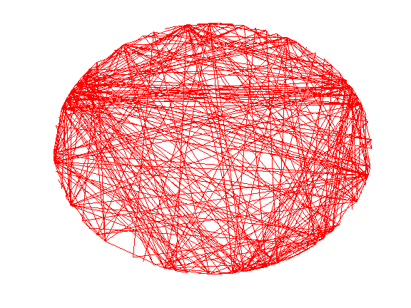
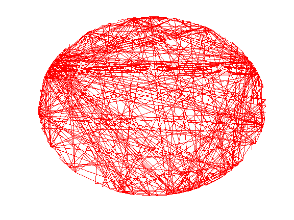
Figure 1: Common edges between C1 and other types identified by methods THP-$\phi_{1}$ (left panel) and THP-$\phi_{2}$ (right panel)

Table 7: Top 10 nodes with highest degrees identified by THP methods in descending order.

Method	Node
THP-$\phi_{1}$	MYD88, NFKB1, CSF2RB, PIK3R5, FAS, PIK3CG, TRADD, BIRC3,
	IL1B, NFKBIA
THP-$\phi_{2}$	NFKB1, MYD88, CSF2RB, PIK3R5, BIRC3, PIK3CG, FAS, IL1B,
	CAPN1, NFKBIA

5 Discussions

In this paper we have introduced the tuning-free heterogeneity pursuit (THP) framework with the chi-based test and the linear functional-based test to detect the heterogeneity in sparsity patterns of multiple networks in the setting of Gaussian graphical models. Such a framework is not only scalable to large scales, but also enjoys optimality properties in the scenario where the number of networks is allowed to diverge and the number of features can be much larger than the sample size. Our theoretical justifications show that under mild regularity conditions, the linear functional-based test has the minimum requirement on the sample size.

Yet the optimality of the sample size requirement for the chi-based test, that is, the minimum sample size requirement with the optimal separating rate $\epsilon_{n}=\mathchoice{{\hbox{$\displaystyle\sqrt{k^{1/2}/n^{(0)}\,}$}\lower 0.4pt\hbox{\vrule height=9.04445pt,depth=-7.2356pt}}}{{\hbox{$\textstyle\sqrt{k^{1/2}/n^{(0)}\,}$}\lower 0.4pt\hbox{\vrule height=9.04445pt,depth=-7.2356pt}}}{{\hbox{$\scriptstyle\sqrt{k^{1/2}/n^{(0)}\,}$}\lower 0.4pt\hbox{\vrule height=6.3611pt,depth=-5.08891pt}}}{{\hbox{$\scriptscriptstyle\sqrt{k^{1/2}/n^{(0)}\,}$}\lower 0.4pt\hbox{\vrule height=4.97221pt,depth=-3.9778pt}}}$ for testing null $H_{0,ab}$ against alternative $H^{l2}_{1,ab}$, still remains as an open problem for future invesigation. The main challenges lie in the need of constructing a new lower bound as in Theorem 4 for alternative $H^{l1}_{1,ab}$, which involves both the sample size requirement and the separating rate. Moreover, the technical analysis in the proof of Theorem 1 contains a relatively loose bound between the $\ell_{1}$ and $\ell_{2}$ norms, which implies that the sample size requirement imposed in Proposition 1 may not be sharp, though sharper than that for the naive combination testing procedure discussed in Section 2.3.

As mentioned in the Introduction, our paper has focused only on two particular aspects of heterogeneity which are the heterogeneity in sparsity patterns over multiple networks and the heterogeneity in noise levels over multiple subpopulations. The appealing features of our THP framework for addressing these issues are empowered by our newly suggested convex approach of heterogeneous group square-root Lasso (HGSL) for the setting of high-dimensional multi-response regression with heterogeneous noises. Other aspects of heterogeneous learning and inference can certainly be interesting as well. For example, in practice one might be interested in studying whether the entries across different graphs are identical or not, that is, the heterogeneity in link strengths. This is a more general yet more challenging problem that deserves further study. Some efforts along this direction have been made in the literature. For instance, Danaher et al. (2014) proposed a penalized likelihood method using the fused Lasso to estimate the common link strength among multiple Gaussian graphs. This method, however, focuses only on the estimation of common link strength and lacks theoretical justification for its performance. Moreover, their proposed algorithm is not scalable due to the complicated form of the likelihood function. Thus it would be interesting to extend the methods developed in our paper to the problem of testing for heterogeneity in link strengths.

Our studies are only among the first attempts to address the challenging issues of heterogeneity in multiple networks in the setting of Gaussian graphical models. It would be interesting to extend our inferential approach to the settings of multiple matrix graphical models, multiple tensor graphical models, and multiple non-Gaussian graphical models, as well as other network models beyond graphical models. Furthermore, the false discovery rate (FDR) control (Benjamini and Hochberg, 1995; Barber and Candès, 2015) is often an important issue in practice. It would also be interesting to further extend the THP framework to provide tools that can control the FDR in multiple networks effectively. In some applications, it is possible that a fraction of the class labels for the subpopulations or even all the class labels can be unavailable, in which clustering techniques can play a crucial role. In addition, there can exist some latent features which would require a broader class of network structures. The developments on heterogeneity identification in multiple networks can also motivate new approaches for regression and classification problems that have networks as an input. The possible extensions addressing these issues are beyond the scope of the current paper and will be interesting topics for future research.

This Supplementary Material contains the proofs of Theorems 1–6 and Propositions 1–3 in Section A, as well as the proofs of key lemmas and additional technical details in Sections B and C, respectively.

Appendix A Proofs of main results

A.1 Proofs of Theorem 1 and Proposition 1

The proofs of Theorems 1–2 and Propositions 1–2 rely on two key sets of results in Lemmas 1 and 2 in Sections B.1 and B.2, respectively, where we use the compact notation $[\ell]$ to denote the set $\{1,\cdots,\ell\}$ for any positive integer $\ell$ whenever there is no confusion. Our results are important consequences of Lemmas 1 and 2. Indeed, it holds that

$$\sum_{t=1}^{k}\left|\mathchoice{{\hbox{$\displaystyle\sqrt{n^{(t)}\hat{\omega}_{2,2}^{(t)}\hat{\omega}_{1,1}^{(t)}\,}$}\lower 0.4pt\hbox{\vrule height=9.32224pt,depth=-7.45782pt}}}{{\hbox{$\textstyle\sqrt{n^{(t)}\hat{\omega}_{2,2}^{(t)}\hat{\omega}_{1,1}^{(t)}\,}$}\lower 0.4pt\hbox{\vrule height=9.32224pt,depth=-7.45782pt}}}{{\hbox{$\scriptstyle\sqrt{n^{(t)}\hat{\omega}_{2,2}^{(t)}\hat{\omega}_{1,1}^{(t)}\,}$}\lower 0.4pt\hbox{\vrule height=8.72223pt,depth=-6.97781pt}}}{{\hbox{$\scriptscriptstyle\sqrt{n^{(t)}\hat{\omega}_{2,2}^{(t)}\hat{\omega}_{1,1}^{(t)}\,}$}\lower 0.4pt\hbox{\vrule height=8.72223pt,depth=-6.97781pt}}}\left(T_{n,k,1,2}^{(t)}-J_{n,k,1,2}^{(t)}\right)-V_{n,k,1,2}^{\ast(t)}\right|\leq T_{1}+T_{2},$$

where

$$T_{1} = \sum_{t=1}^{k}\mathchoice{{\hbox{$\displaystyle\sqrt{n^{(t)}\hat{\omega}_{2,2}^{(t)}\hat{\omega}_{1,1}^{(t)}\,}$}\lower 0.4pt\hbox{\vrule height=9.32224pt,depth=-7.45782pt}}}{{\hbox{$\textstyle\sqrt{n^{(t)}\hat{\omega}_{2,2}^{(t)}\hat{\omega}_{1,1}^{(t)}\,}$}\lower 0.4pt\hbox{\vrule height=9.32224pt,depth=-7.45782pt}}}{{\hbox{$\scriptstyle\sqrt{n^{(t)}\hat{\omega}_{2,2}^{(t)}\hat{\omega}_{1,1}^{(t)}\,}$}\lower 0.4pt\hbox{\vrule height=8.72223pt,depth=-6.97781pt}}}{{\hbox{$\scriptscriptstyle\sqrt{n^{(t)}\hat{\omega}_{2,2}^{(t)}\hat{\omega}_{1,1}^{(t)}\,}$}\lower 0.4pt\hbox{\vrule height=8.72223pt,depth=-6.97781pt}}}\left|T_{n,k,1,2}^{(t)}-J_{n,k,1,2}^{(t)}-\frac{1}{n^{(t)}}\sum_{i=1}^{n^{(t)}}\left(E_{i,1}^{(t)}E_{i,2}^{(t)}-\mathbb{E}E_{i,1}^{(t)}E_{i,2}^{(t)}\right)\right|,$$

$$T_{2} = \sum_{t=1}^{k}\left|1-\mathchoice{{\hbox{$\displaystyle\sqrt{\frac{\hat{\omega}_{2,2}^{(t)}\hat{\omega}_{1,1}^{(t)}}{\omega_{2,2}^{(t)}\tilde{\omega}_{1,1}^{(t)}}\,}$}\lower 0.4pt\hbox{\vrule height=18.32333pt,depth=-14.65874pt}}}{{\hbox{$\textstyle\sqrt{\frac{\hat{\omega}_{2,2}^{(t)}\hat{\omega}_{1,1}^{(t)}}{\omega_{2,2}^{(t)}\tilde{\omega}_{1,1}^{(t)}}\,}$}\lower 0.4pt\hbox{\vrule height=16.18332pt,depth=-12.94672pt}}}{{\hbox{$\scriptstyle\sqrt{\frac{\hat{\omega}_{2,2}^{(t)}\hat{\omega}_{1,1}^{(t)}}{\omega_{2,2}^{(t)}\tilde{\omega}_{1,1}^{(t)}}\,}$}\lower 0.4pt\hbox{\vrule height=16.18332pt,depth=-12.94672pt}}}{{\hbox{$\scriptscriptstyle\sqrt{\frac{\hat{\omega}_{2,2}^{(t)}\hat{\omega}_{1,1}^{(t)}}{\omega_{2,2}^{(t)}\tilde{\omega}_{1,1}^{(t)}}\,}$}\lower 0.4pt\hbox{\vrule height=16.18332pt,depth=-12.94672pt}}}\right|\left|\mathchoice{{\hbox{$\displaystyle\sqrt{\frac{\omega_{2,2}^{(t)}\tilde{\omega}_{1,1}^{(t)}}{n^{(t)}}\,}$}\lower 0.4pt\hbox{\vrule height=15.41833pt,depth=-12.33472pt}}}{{\hbox{$\textstyle\sqrt{\frac{\omega_{2,2}^{(t)}\tilde{\omega}_{1,1}^{(t)}}{n^{(t)}}\,}$}\lower 0.4pt\hbox{\vrule height=13.04582pt,depth=-10.4367pt}}}{{\hbox{$\scriptstyle\sqrt{\frac{\omega_{2,2}^{(t)}\tilde{\omega}_{1,1}^{(t)}}{n^{(t)}}\,}$}\lower 0.4pt\hbox{\vrule height=12.61526pt,depth=-10.09225pt}}}{{\hbox{$\scriptscriptstyle\sqrt{\frac{\omega_{2,2}^{(t)}\tilde{\omega}_{1,1}^{(t)}}{n^{(t)}}\,}$}\lower 0.4pt\hbox{\vrule height=12.61526pt,depth=-10.09225pt}}}\sum_{i=1}^{n^{(t)}}\left(E_{i,1}^{(t)}E_{i,2}^{(t)}-\mathbb{E}E_{i,1}^{(t)}E_{i,2}^{(t)}\right)\right|.$$

According to Lemma 1, we have $|\hat{\omega}_{j,j}^{(t)}-\omega_{j,j}^{(t)}|\leq C^{\prime}(\mathchoice{{\hbox{$\displaystyle\sqrt{\frac{\log(k/\delta_{1})}{n^{(0)}}\,}$}\lower 0.4pt\hbox{\vrule height=13.20277pt,depth=-10.56227pt}}}{{\hbox{$\textstyle\sqrt{\frac{\log(k/\delta_{1})}{n^{(0)}}\,}$}\lower 0.4pt\hbox{\vrule height=9.25694pt,depth=-7.4056pt}}}{{\hbox{$\scriptstyle\sqrt{\frac{\log(k/\delta_{1})}{n^{(0)}}\,}$}\lower 0.4pt\hbox{\vrule height=6.86526pt,depth=-5.49223pt}}}{{\hbox{$\scriptscriptstyle\sqrt{\frac{\log(k/\delta_{1})}{n^{(0)}}\,}$}\lower 0.4pt\hbox{\vrule height=6.86526pt,depth=-5.49223pt}}}+s\frac{\left(k+\log p\right)}{n^{(0)}})=o(1)$ with probability at least $1-6p^{1-\delta}-2\delta_{1}$ uniformly for all $t\in[k]$ and $j=1,2$. Therefore, Condition 1 implies that all $\hat{\omega}_{j,j}^{(t)}$ are bounded from both below and above, which together with Lemma 2 and $s\left(k+\log p\right)/n^{(0)}=o(1)$ leads to

$$T_{1}\leq C\left(s\frac{k+(\log p)}{\mathchoice{{\hbox{$\displaystyle\sqrt{n^{(0)}\,}$}\lower 0.4pt\hbox{\vrule height=6.40555pt,depth=-5.12447pt}}}{{\hbox{$\textstyle\sqrt{n^{(0)}\,}$}\lower 0.4pt\hbox{\vrule height=6.40555pt,depth=-5.12447pt}}}{{\hbox{$\scriptstyle\sqrt{n^{(0)}\,}$}\lower 0.4pt\hbox{\vrule height=4.51389pt,depth=-3.61113pt}}}{{\hbox{$\scriptscriptstyle\sqrt{n^{(0)}\,}$}\lower 0.4pt\hbox{\vrule height=3.65277pt,depth=-2.92224pt}}}}\right)$$

with probability at least $1-12p^{1-\delta}-2\delta_{1}$, where positive constant $C$ depends on constants $M,M_{0},\delta,C_{1},\\ C_{2}$, and $C_{3}$.

It remains to upper bound term $T_{2}$. Note that Lemma 1 together with Condition 1 implies that $\tilde{\omega}_{1,1}^{(t)}$ is bounded. In addition, Condition 1 also implies that $E_{i,1}^{(t)}E_{i,2}^{(t)}$, $i\in[n^{(t)}]$ are i.i.d. sub-exponential with bounded constant parameter. Consequently, Bernstein’s inequality (see, e.g., Proposition 5.16, Vershynin (2010)) entails immediately that $\max_{k}|V_{n,k,1,2}^{\ast(t)}|<\mathchoice{{\hbox{$\displaystyle\sqrt{C^{\prime}\log(k/\delta_{1})\,}$}\lower 0.4pt\hbox{\vrule height=8.38887pt,depth=-6.71114pt}}}{{\hbox{$\textstyle\sqrt{C^{\prime}\log(k/\delta_{1})\,}$}\lower 0.4pt\hbox{\vrule height=8.38887pt,depth=-6.71114pt}}}{{\hbox{$\scriptstyle\sqrt{C^{\prime}\log(k/\delta_{1})\,}$}\lower 0.4pt\hbox{\vrule height=5.89444pt,depth=-4.71558pt}}}{{\hbox{$\scriptscriptstyle\sqrt{C^{\prime}\log(k/\delta_{1})\,}$}\lower 0.4pt\hbox{\vrule height=4.52777pt,depth=-3.62224pt}}}$ with probability at least $1-2\delta_{1}$, where positive constant $C^{\prime}$ depends on $M$ only. Therefore, this fact and Lemma 1 along with the union bound further yield with probability at least $1-6p^{1-\delta}-4\delta_{1}$ that

$$T_{2} \leq \mathchoice{{\hbox{$\displaystyle\sqrt{C^{\prime}\log(k/\delta_{1})\,}$}\lower 0.4pt\hbox{\vrule height=8.38887pt,depth=-6.71114pt}}}{{\hbox{$\textstyle\sqrt{C^{\prime}\log(k/\delta_{1})\,}$}\lower 0.4pt\hbox{\vrule height=8.38887pt,depth=-6.71114pt}}}{{\hbox{$\scriptstyle\sqrt{C^{\prime}\log(k/\delta_{1})\,}$}\lower 0.4pt\hbox{\vrule height=5.89444pt,depth=-4.71558pt}}}{{\hbox{$\scriptscriptstyle\sqrt{C^{\prime}\log(k/\delta_{1})\,}$}\lower 0.4pt\hbox{\vrule height=4.52777pt,depth=-3.62224pt}}}\sum_{t=1}^{k}\left|1-\mathchoice{{\hbox{$\displaystyle\sqrt{\frac{\hat{\omega}_{2,2}^{(t)}\hat{\omega}_{1,1}^{(t)}}{\omega_{2,2}^{(t)}\tilde{\omega}_{1,1}^{(t)}}\,}$}\lower 0.4pt\hbox{\vrule height=18.32333pt,depth=-14.65874pt}}}{{\hbox{$\textstyle\sqrt{\frac{\hat{\omega}_{2,2}^{(t)}\hat{\omega}_{1,1}^{(t)}}{\omega_{2,2}^{(t)}\tilde{\omega}_{1,1}^{(t)}}\,}$}\lower 0.4pt\hbox{\vrule height=16.18332pt,depth=-12.94672pt}}}{{\hbox{$\scriptstyle\sqrt{\frac{\hat{\omega}_{2,2}^{(t)}\hat{\omega}_{1,1}^{(t)}}{\omega_{2,2}^{(t)}\tilde{\omega}_{1,1}^{(t)}}\,}$}\lower 0.4pt\hbox{\vrule height=16.18332pt,depth=-12.94672pt}}}{{\hbox{$\scriptscriptstyle\sqrt{\frac{\hat{\omega}_{2,2}^{(t)}\hat{\omega}_{1,1}^{(t)}}{\omega_{2,2}^{(t)}\tilde{\omega}_{1,1}^{(t)}}\,}$}\lower 0.4pt\hbox{\vrule height=16.18332pt,depth=-12.94672pt}}}\right|$$

$$\leq C\mathchoice{{\hbox{$\displaystyle\sqrt{\log(k/\delta_{1})\,}$}\lower 0.4pt\hbox{\vrule height=7.5pt,depth=-6.00003pt}}}{{\hbox{$\textstyle\sqrt{\log(k/\delta_{1})\,}$}\lower 0.4pt\hbox{\vrule height=7.5pt,depth=-6.00003pt}}}{{\hbox{$\scriptstyle\sqrt{\log(k/\delta_{1})\,}$}\lower 0.4pt\hbox{\vrule height=5.25pt,depth=-4.20003pt}}}{{\hbox{$\scriptscriptstyle\sqrt{\log(k/\delta_{1})\,}$}\lower 0.4pt\hbox{\vrule height=3.75pt,depth=-3.00002pt}}}\left(\sum_{t=1}^{k}\left|\tilde{\omega}_{1,1}^{(t)}-\hat{\omega}_{1,1}^{(t)}\right|+\sum_{t=1}^{k}\left|\omega_{2,2}^{(t)}-\hat{\omega}_{2,2}^{(t)}\right|\right)$$

$$\leq C\left(k\mathchoice{{\hbox{$\displaystyle\sqrt{\frac{\log(k/\delta_{1})}{n^{(0)}}\,}$}\lower 0.4pt\hbox{\vrule height=13.20277pt,depth=-10.56227pt}}}{{\hbox{$\textstyle\sqrt{\frac{\log(k/\delta_{1})}{n^{(0)}}\,}$}\lower 0.4pt\hbox{\vrule height=9.25694pt,depth=-7.4056pt}}}{{\hbox{$\scriptstyle\sqrt{\frac{\log(k/\delta_{1})}{n^{(0)}}\,}$}\lower 0.4pt\hbox{\vrule height=6.86526pt,depth=-5.49223pt}}}{{\hbox{$\scriptscriptstyle\sqrt{\frac{\log(k/\delta_{1})}{n^{(0)}}\,}$}\lower 0.4pt\hbox{\vrule height=6.86526pt,depth=-5.49223pt}}}+s\frac{\left(k+(\log p)\right)}{n^{(0)}}\right)\mathchoice{{\hbox{$\displaystyle\sqrt{\log(k/\delta_{1})\,}$}\lower 0.4pt\hbox{\vrule height=7.5pt,depth=-6.00003pt}}}{{\hbox{$\textstyle\sqrt{\log(k/\delta_{1})\,}$}\lower 0.4pt\hbox{\vrule height=7.5pt,depth=-6.00003pt}}}{{\hbox{$\scriptstyle\sqrt{\log(k/\delta_{1})\,}$}\lower 0.4pt\hbox{\vrule height=5.25pt,depth=-4.20003pt}}}{{\hbox{$\scriptscriptstyle\sqrt{\log(k/\delta_{1})\,}$}\lower 0.4pt\hbox{\vrule height=3.75pt,depth=-3.00002pt}}}$$

$$\leq C(s\frac{k+(\log p)}{\mathchoice{{\hbox{$\displaystyle\sqrt{n^{(0)}\,}$}\lower 0.4pt\hbox{\vrule height=6.40555pt,depth=-5.12447pt}}}{{\hbox{$\textstyle\sqrt{n^{(0)}\,}$}\lower 0.4pt\hbox{\vrule height=6.40555pt,depth=-5.12447pt}}}{{\hbox{$\scriptstyle\sqrt{n^{(0)}\,}$}\lower 0.4pt\hbox{\vrule height=4.51389pt,depth=-3.61113pt}}}{{\hbox{$\scriptscriptstyle\sqrt{n^{(0)}\,}$}\lower 0.4pt\hbox{\vrule height=3.65277pt,depth=-2.92224pt}}}}),$$

where the second inequality follows from the fact that all $\hat{\omega}_{j,j}^{(t)},$ $\tilde{\omega}_{j,j}^{(t)}$, and $\omega_{j,j}^{(t)}$ are bounded from both below and above, the third inequality is due to Lemma 1, and the last inequality follows from our sample size assumptions $\log(k/\delta_{1})=O(s(1+(\log p)/k))$ as well as $\log(k/\delta_{1})=o(n^{(0)})$. The positive constant $C$ above depends on constants $M,\delta,C_{1},C_{2}$, and $C_{3}$.

Combining the bounds of $T_{1}$ and $T_{2}$ above, we deduce that the following inequality holds with probability at least $1-12p^{1-\delta}-4\delta_{1}$,

$$\sum_{t=1}^{k}\left|\mathchoice{{\hbox{$\displaystyle\sqrt{n^{(t)}\hat{\omega}_{2,2}^{(t)}\hat{\omega}_{1,1}^{(t)}\,}$}\lower 0.4pt\hbox{\vrule height=9.32224pt,depth=-7.45782pt}}}{{\hbox{$\textstyle\sqrt{n^{(t)}\hat{\omega}_{2,2}^{(t)}\hat{\omega}_{1,1}^{(t)}\,}$}\lower 0.4pt\hbox{\vrule height=9.32224pt,depth=-7.45782pt}}}{{\hbox{$\scriptstyle\sqrt{n^{(t)}\hat{\omega}_{2,2}^{(t)}\hat{\omega}_{1,1}^{(t)}\,}$}\lower 0.4pt\hbox{\vrule height=8.72223pt,depth=-6.97781pt}}}{{\hbox{$\scriptscriptstyle\sqrt{n^{(t)}\hat{\omega}_{2,2}^{(t)}\hat{\omega}_{1,1}^{(t)}\,}$}\lower 0.4pt\hbox{\vrule height=8.72223pt,depth=-6.97781pt}}}\left(T_{n,k,1,2}^{(t)}-J_{n,k,1,2}^{(t)}\right)-V_{n,k,1,2}^{\ast(t)}\right|\leq C\left(s\frac{k+\log p}{\mathchoice{{\hbox{$\displaystyle\sqrt{n^{(0)}\,}$}\lower 0.4pt\hbox{\vrule height=6.40555pt,depth=-5.12447pt}}}{{\hbox{$\textstyle\sqrt{n^{(0)}\,}$}\lower 0.4pt\hbox{\vrule height=6.40555pt,depth=-5.12447pt}}}{{\hbox{$\scriptstyle\sqrt{n^{(0)}\,}$}\lower 0.4pt\hbox{\vrule height=4.51389pt,depth=-3.61113pt}}}{{\hbox{$\scriptscriptstyle\sqrt{n^{(0)}\,}$}\lower 0.4pt\hbox{\vrule height=3.65277pt,depth=-2.92224pt}}}}\right),$$ (A.1)

where constant $C>0$ depends only on $M,M_{0},\delta,C_{1},C_{2}$, and $C_{3}$.

Aided with the key result in (A.1) above, the analysis of Theorem 1 is straightforward. Indeed we have

$$\left|\left(\sum_{t=1}^{k}n^{(t)}\hat{\omega}_{2,2}^{(t)}\hat{\omega}_{1,1}^{(t)}\left(T_{n,k,1,2}^{(t)}-J_{n,k,1,2}^{(t)}\right)^{2}\right)^{1/2}-U_{n,k,1,2}^{\ast}\right|$$

$$\leq \left[\sum_{t=1}^{k}\left(\mathchoice{{\hbox{$\displaystyle\sqrt{n^{(t)}\hat{\omega}_{2,2}^{(t)}\hat{\omega}_{1,1}^{(t)}\,}$}\lower 0.4pt\hbox{\vrule height=9.32224pt,depth=-7.45782pt}}}{{\hbox{$\textstyle\sqrt{n^{(t)}\hat{\omega}_{2,2}^{(t)}\hat{\omega}_{1,1}^{(t)}\,}$}\lower 0.4pt\hbox{\vrule height=9.32224pt,depth=-7.45782pt}}}{{\hbox{$\scriptstyle\sqrt{n^{(t)}\hat{\omega}_{2,2}^{(t)}\hat{\omega}_{1,1}^{(t)}\,}$}\lower 0.4pt\hbox{\vrule height=8.72223pt,depth=-6.97781pt}}}{{\hbox{$\scriptscriptstyle\sqrt{n^{(t)}\hat{\omega}_{2,2}^{(t)}\hat{\omega}_{1,1}^{(t)}\,}$}\lower 0.4pt\hbox{\vrule height=8.72223pt,depth=-6.97781pt}}}\left(T_{n,k,1,2}^{(t)}-J_{n,k,1,2}^{(t)}\right)-V_{n,k,1,2}^{\ast(t)}\right)^{2}\right]^{1/2}$$

$$\leq \sum_{t=1}^{k}\left|\mathchoice{{\hbox{$\displaystyle\sqrt{n^{(t)}\hat{\omega}_{2,2}^{(t)}\hat{\omega}_{1,1}^{(t)}\,}$}\lower 0.4pt\hbox{\vrule height=9.32224pt,depth=-7.45782pt}}}{{\hbox{$\textstyle\sqrt{n^{(t)}\hat{\omega}_{2,2}^{(t)}\hat{\omega}_{1,1}^{(t)}\,}$}\lower 0.4pt\hbox{\vrule height=9.32224pt,depth=-7.45782pt}}}{{\hbox{$\scriptstyle\sqrt{n^{(t)}\hat{\omega}_{2,2}^{(t)}\hat{\omega}_{1,1}^{(t)}\,}$}\lower 0.4pt\hbox{\vrule height=8.72223pt,depth=-6.97781pt}}}{{\hbox{$\scriptscriptstyle\sqrt{n^{(t)}\hat{\omega}_{2,2}^{(t)}\hat{\omega}_{1,1}^{(t)}\,}$}\lower 0.4pt\hbox{\vrule height=8.72223pt,depth=-6.97781pt}}}\left(T_{n,k,1,2}^{(t)}-J_{n,k,1,2}^{(t)}\right)-V_{n,k,1,2}^{\ast(t)}\right|$$

$$\leq Cs\frac{k+(\log p)}{\mathchoice{{\hbox{$\displaystyle\sqrt{n^{(0)}\,}$}\lower 0.4pt\hbox{\vrule height=6.40555pt,depth=-5.12447pt}}}{{\hbox{$\textstyle\sqrt{n^{(0)}\,}$}\lower 0.4pt\hbox{\vrule height=6.40555pt,depth=-5.12447pt}}}{{\hbox{$\scriptstyle\sqrt{n^{(0)}\,}$}\lower 0.4pt\hbox{\vrule height=4.51389pt,depth=-3.61113pt}}}{{\hbox{$\scriptscriptstyle\sqrt{n^{(0)}\,}$}\lower 0.4pt\hbox{\vrule height=3.65277pt,depth=-2.92224pt}}}},$$

where the last inequality is due to (A.1). The remaining part of the proof for Theorem 1 follows easily.

Note that the chi distribution $U_{n,k,1,2}^{\ast}$ always has constant level standard deviation. Hence Proposition 1 follows from the fact that the error bound of $|U_{n,k,1,2}-U_{n,k,1,2}^{\ast}|$ is $o(1)$ with significant probability under the sample size assumption, which completes the proofs.

A.2 Proofs of Theorem 2 and Proposition 2

Theorem 2 is an immediate consequence of (A.1) established in Section A.1, since the left-hand side of (A.1) is an upper bound of the left-hand side of (36) regardless of what sign vector is picked.

Note that $V_{n,k,1,2}^{\ast}(\xi)$ follows distribution $N(0,k)$. The error bound of $|V_{n,k,1,2}(\xi)-V_{n,k,1,2}^{\ast}(\xi)|$ is negligible compared to the standard deviation of $V_{n,k,1,2}^{\ast}(\xi)$ with significant probability under the sample size assumption, that is, $s(k+(\log p))/\mathchoice{{\hbox{$\displaystyle\sqrt{n^{(0)}\,}$}\lower 0.4pt\hbox{\vrule height=6.40555pt,depth=-5.12447pt}}}{{\hbox{$\textstyle\sqrt{n^{(0)}\,}$}\lower 0.4pt\hbox{\vrule height=6.40555pt,depth=-5.12447pt}}}{{\hbox{$\scriptstyle\sqrt{n^{(0)}\,}$}\lower 0.4pt\hbox{\vrule height=4.51389pt,depth=-3.61113pt}}}{{\hbox{$\scriptscriptstyle\sqrt{n^{(0)}\,}$}\lower 0.4pt\hbox{\vrule height=3.65277pt,depth=-2.92224pt}}}=o(k^{1/2})$, which concludes the proofs of both Theorem 2 and Proposition 2.

A.3 Proof of Theorem 3

The first part of the analysis serves as a general tool for both the lower bound arguments in Theorem 3 and the proof of Theorem 4. It suffices to assume without loss of generality that the sample sizes of all $k$ graphs are identical, that is, $n^{(1)}=\cdots=n^{(k)}=n^{(0)}$, noting that Condition 2 is valid under this setting. Consider a least favorable finite subset $\mathcal{G}=\{\Omega_{1}^{0},\cdots,\Omega_{m}^{0}\}\subset\mathcal{A}$ in the alternative sets, where $\mathcal{A=A}^{l2}(s,c^{\prime}\mathchoice{{\hbox{$\displaystyle\sqrt{k^{1/2}/n^{(0)}\,}$}\lower 0.4pt\hbox{\vrule height=9.04445pt,depth=-7.2356pt}}}{{\hbox{$\textstyle\sqrt{k^{1/2}/n^{(0)}\,}$}\lower 0.4pt\hbox{\vrule height=9.04445pt,depth=-7.2356pt}}}{{\hbox{$\scriptstyle\sqrt{k^{1/2}/n^{(0)}\,}$}\lower 0.4pt\hbox{\vrule height=6.3611pt,depth=-5.08891pt}}}{{\hbox{$\scriptscriptstyle\sqrt{k^{1/2}/n^{(0)}\,}$}\lower 0.4pt\hbox{\vrule height=4.97221pt,depth=-3.9778pt}}})$ for Theorem 3 (1), $\mathcal{A=A}^{l1}(s,c^{\prime}\mathchoice{{\hbox{$\displaystyle\sqrt{k/n^{(0)}\,}$}\lower 0.4pt\hbox{\vrule height=7.5pt,depth=-6.00003pt}}}{{\hbox{$\textstyle\sqrt{k/n^{(0)}\,}$}\lower 0.4pt\hbox{\vrule height=7.5pt,depth=-6.00003pt}}}{{\hbox{$\scriptstyle\sqrt{k/n^{(0)}\,}$}\lower 0.4pt\hbox{\vrule height=5.25pt,depth=-4.20003pt}}}{{\hbox{$\scriptscriptstyle\sqrt{k/n^{(0)}\,}$}\lower 0.4pt\hbox{\vrule height=3.75pt,depth=-3.00002pt}}},\xi)$ for Theorem 3 (2), and $\mathcal{A=A}^{l1}(s,c\mathchoice{{\hbox{$\displaystyle\sqrt{k/n^{(0)}\,}$}\lower 0.4pt\hbox{\vrule height=7.5pt,depth=-6.00003pt}}}{{\hbox{$\textstyle\sqrt{k/n^{(0)}\,}$}\lower 0.4pt\hbox{\vrule height=7.5pt,depth=-6.00003pt}}}{{\hbox{$\scriptstyle\sqrt{k/n^{(0)}\,}$}\lower 0.4pt\hbox{\vrule height=5.25pt,depth=-4.20003pt}}}{{\hbox{$\scriptscriptstyle\sqrt{k/n^{(0)}\,}$}\lower 0.4pt\hbox{\vrule height=3.75pt,depth=-3.00002pt}}},\xi)$ for Theorem 4. In addition, we consider one element in $\Omega_{0}^{0}\in\mathcal{N}(s)$.  The choice of $\mathcal{G}$ and $\Omega_{0}^{0}$ will be determined later.

Recall that each index denotes each of the $k$ graphs, that is, $\Omega_{h}^{0}=\{\Omega_{h}^{(t)}\}_{t=1}^{k}$ for $h=0,\cdots,m$. Let $\mathbb{P}_{h}\equiv\mathbb{P}_{\Omega_{h}^{0}}$ denote the joint distribution of the observations when the true parameter is $\Omega_{h}^{0}$. In other words, $\mathbb{P}_{h}$ is the joint distribution of $n^{(0)}$ copies of $k$ graphs $\prod\nolimits_{t=1}^{k}g_{h}^{(t)}(x_{t})$, where $g_{h}^{(t)}(\cdot)$ is the density of $N(0,(\Omega_{h}^{(t)})^{-1})$ for $t\in[k]$. We use $\mathbb{E}_{v}$ and $f_{h}$ to denote the expectation under $\mathbb{P}_{v}$ and the density function under $\mathbb{P}_{h}$, respectively. Moreover, let $\mathbb{\bar{P}}=\frac{1}{m}\sum_{h=1}^{m}\mathbb{P}_{h}$ be the average measure of these joint distributions indexed by elements in $\mathcal{G}$. For any test $\psi_{0}$, we have

$$\sup_{v\in\mathcal{G}}\left(\mathbb{E}_{0}\psi_{0}+\mathbb{E}_{v}(1-\psi_{0})\right) \geq \inf_{\psi}\left(\sup_{v\in\mathcal{G}}\mathbb{E}_{0}\psi+\mathbb{E}_{v}(1-\psi)\right)$$

$$\geq \inf_{\psi}\left(\mathbb{E}_{0}\psi+\mathbb{\bar{E}}(1-\psi)\right)$$

$$= \left\|\mathbb{P}_{0}\wedge\mathbb{\bar{P}}\right\|,$$

where $\|\mathbb{P}_{0}\wedge\mathbb{\bar{P}}\|$ is the total variation affinity between two measures. Therefore, if $\psi_{0}$ has significance level $\alpha$ it holds that

$$\inf_{v\in\mathcal{A}}\mathbb{P}_{v}(\psi_{0}\mbox{ \rm rejects }H_{0,12})\leq\inf_{v\in\mathcal{G}}\mathbb{E}_{v}(\psi_{0})\leq 1+\alpha-\left\|\mathbb{P}_{0}\wedge\mathbb{\bar{P}}\right\|\mbox{\rm.}$$ (A.2)

To show that for any given $\beta>\alpha$ and some constant $c>0$, no test of significance level $\alpha$ satisfies (42), it is sufficient to prove that $\|\mathbb{P}_{0}\wedge\mathbb{\bar{P}}\|>1-(\beta-\alpha)/2$, which together with (A.2) implies that

$$\inf_{v\in\mathcal{A}}\mathbb{P}_{v}(\psi_{0}\mbox{ \rm rejects }H_{0,12})\leq\beta-(\beta-\alpha)/2.$$

We will use this fact in the lower bound arguments in Theorem 3 and the proof of Theorem 4 with different constructions of $\mathcal{G}$ and $\Omega_{0}^{0}$, and constant $c>0$.

A.3.1 Proof of Theorem 3 (1)

To show that $\epsilon_{n}=\mathchoice{{\hbox{$\displaystyle\sqrt{k^{1/2}/n^{(0)}\,}$}\lower 0.4pt\hbox{\vrule height=9.04445pt,depth=-7.2356pt}}}{{\hbox{$\textstyle\sqrt{k^{1/2}/n^{(0)}\,}$}\lower 0.4pt\hbox{\vrule height=9.04445pt,depth=-7.2356pt}}}{{\hbox{$\scriptstyle\sqrt{k^{1/2}/n^{(0)}\,}$}\lower 0.4pt\hbox{\vrule height=6.3611pt,depth=-5.08891pt}}}{{\hbox{$\scriptscriptstyle\sqrt{k^{1/2}/n^{(0)}\,}$}\lower 0.4pt\hbox{\vrule height=4.97221pt,depth=-3.9778pt}}}$ is the separating rate, we first establish the lower bound (43) and then prove that our test $\phi_{2}$ satisfies (42) with $\mathcal{A}=\mathcal{A}^{l2}(s,c\mathchoice{{\hbox{$\displaystyle\sqrt{k^{1/2}/n^{(0)}\,}$}\lower 0.4pt\hbox{\vrule height=9.04445pt,depth=-7.2356pt}}}{{\hbox{$\textstyle\sqrt{k^{1/2}/n^{(0)}\,}$}\lower 0.4pt\hbox{\vrule height=9.04445pt,depth=-7.2356pt}}}{{\hbox{$\scriptstyle\sqrt{k^{1/2}/n^{(0)}\,}$}\lower 0.4pt\hbox{\vrule height=6.3611pt,depth=-5.08891pt}}}{{\hbox{$\scriptscriptstyle\sqrt{k^{1/2}/n^{(0)}\,}$}\lower 0.4pt\hbox{\vrule height=4.97221pt,depth=-3.9778pt}}})$. With the aid of (A.2), it suffices to show that for fixed $\beta>\alpha$, there exists some constant $c^{\prime}>0$ such that $\|\mathbb{P}_{0}\wedge\mathbb{\bar{P}}\|>1-(\beta-\alpha)/2$ with appropriate choices of $\mathcal{G}\subset\mathcal{A=A}^{l2}(s,c^{\prime}\mathchoice{{\hbox{$\displaystyle\sqrt{k^{1/2}/n^{(0)}\,}$}\lower 0.4pt\hbox{\vrule height=9.04445pt,depth=-7.2356pt}}}{{\hbox{$\textstyle\sqrt{k^{1/2}/n^{(0)}\,}$}\lower 0.4pt\hbox{\vrule height=9.04445pt,depth=-7.2356pt}}}{{\hbox{$\scriptstyle\sqrt{k^{1/2}/n^{(0)}\,}$}\lower 0.4pt\hbox{\vrule height=6.3611pt,depth=-5.08891pt}}}{{\hbox{$\scriptscriptstyle\sqrt{k^{1/2}/n^{(0)}\,}$}\lower 0.4pt\hbox{\vrule height=4.97221pt,depth=-3.9778pt}}})$ and $\Omega_{0}^{0}\in\mathcal{N}(s)$.

We define

$$\Omega_{0}^{0}=\{\Omega_{0}^{(t)}\}_{t=1}^{k}\text{ \ such that \ }\Omega_{0}^{(1)}=\cdots=\Omega_{0}^{(k)}=I.$$ (A.3)

For simplicity, assume that $\tau\mathchoice{{\hbox{$\displaystyle\sqrt{k\,}$}\lower 0.4pt\hbox{\vrule height=6.94444pt,depth=-5.55559pt}}}{{\hbox{$\textstyle\sqrt{k\,}$}\lower 0.4pt\hbox{\vrule height=6.94444pt,depth=-5.55559pt}}}{{\hbox{$\scriptstyle\sqrt{k\,}$}\lower 0.4pt\hbox{\vrule height=4.8611pt,depth=-3.8889pt}}}{{\hbox{$\scriptscriptstyle\sqrt{k\,}$}\lower 0.4pt\hbox{\vrule height=3.47221pt,depth=-2.77779pt}}}$ is an integer with some small constant $\tau>0$ to be determined later. Otherwise, $\tau\mathchoice{{\hbox{$\displaystyle\sqrt{k\,}$}\lower 0.4pt\hbox{\vrule height=6.94444pt,depth=-5.55559pt}}}{{\hbox{$\textstyle\sqrt{k\,}$}\lower 0.4pt\hbox{\vrule height=6.94444pt,depth=-5.55559pt}}}{{\hbox{$\scriptstyle\sqrt{k\,}$}\lower 0.4pt\hbox{\vrule height=4.8611pt,depth=-3.8889pt}}}{{\hbox{$\scriptscriptstyle\sqrt{k\,}$}\lower 0.4pt\hbox{\vrule height=3.47221pt,depth=-2.77779pt}}}$ can be replaced by its floor function $\lfloor\tau\mathchoice{{\hbox{$\displaystyle\sqrt{k\,}$}\lower 0.4pt\hbox{\vrule height=6.94444pt,depth=-5.55559pt}}}{{\hbox{$\textstyle\sqrt{k\,}$}\lower 0.4pt\hbox{\vrule height=6.94444pt,depth=-5.55559pt}}}{{\hbox{$\scriptstyle\sqrt{k\,}$}\lower 0.4pt\hbox{\vrule height=4.8611pt,depth=-3.8889pt}}}{{\hbox{$\scriptscriptstyle\sqrt{k\,}$}\lower 0.4pt\hbox{\vrule height=3.47221pt,depth=-2.77779pt}}}\rfloor$ in the analysis below. Then we construct a subset

$$\mathcal{G} = \Big{\{}\Omega^{0}=\{\Omega^{(t)}\}_{t=1}^{k}:\mbox{ there exists some }T\subset[k]\mbox{ with }\left|T\right|=\tau\mathchoice{{\hbox{$\displaystyle\sqrt{k\,}$}\lower 0.4pt\hbox{\vrule height=6.94444pt,depth=-5.55559pt}}}{{\hbox{$\textstyle\sqrt{k\,}$}\lower 0.4pt\hbox{\vrule height=6.94444pt,depth=-5.55559pt}}}{{\hbox{$\scriptstyle\sqrt{k\,}$}\lower 0.4pt\hbox{\vrule height=4.8611pt,depth=-3.8889pt}}}{{\hbox{$\scriptscriptstyle\sqrt{k\,}$}\lower 0.4pt\hbox{\vrule height=3.47221pt,depth=-2.77779pt}}}\mbox{ such that }$$ (A.4)

$$\quad\Omega^{(t)}=I\mbox{ for }t\notin T\mbox{ and }(\Omega_{0}^{(k)})^{-1}=I+(n^{(0)})^{-1/2}e_{12}\mbox{ for }t\in T\Big{\}},$$

where $e_{12}$ is the matrix with the $(1,2)$th and $(2,1)$th entries being one and all other entries being zero. Therefore, there are $\binom{k}{\tau\mathchoice{{\hbox{$\displaystyle\sqrt{k\,}$}\lower 0.4pt\hbox{\vrule height=4.8611pt,depth=-3.8889pt}}}{{\hbox{$\textstyle\sqrt{k\,}$}\lower 0.4pt\hbox{\vrule height=4.8611pt,depth=-3.8889pt}}}{{\hbox{$\scriptstyle\sqrt{k\,}$}\lower 0.4pt\hbox{\vrule height=3.40277pt,depth=-2.72223pt}}}{{\hbox{$\scriptscriptstyle\sqrt{k\,}$}\lower 0.4pt\hbox{\vrule height=2.43054pt,depth=-1.94444pt}}}}$ distinct elements in $\mathcal{G}$ and thus $m=\binom{k}{\tau\mathchoice{{\hbox{$\displaystyle\sqrt{k\,}$}\lower 0.4pt\hbox{\vrule height=4.8611pt,depth=-3.8889pt}}}{{\hbox{$\textstyle\sqrt{k\,}$}\lower 0.4pt\hbox{\vrule height=4.8611pt,depth=-3.8889pt}}}{{\hbox{$\scriptstyle\sqrt{k\,}$}\lower 0.4pt\hbox{\vrule height=3.40277pt,depth=-2.72223pt}}}{{\hbox{$\scriptscriptstyle\sqrt{k\,}$}\lower 0.4pt\hbox{\vrule height=2.43054pt,depth=-1.94444pt}}}}$. It is easy to check that $\Omega_{0}^{0}\in\mathcal{N}(s)$ and $\mathcal{G\subset A}^{l2}(s,c^{\prime}\mathchoice{{\hbox{$\displaystyle\sqrt{k^{1/2}/n^{(0)}\,}$}\lower 0.4pt\hbox{\vrule height=9.04445pt,depth=-7.2356pt}}}{{\hbox{$\textstyle\sqrt{k^{1/2}/n^{(0)}\,}$}\lower 0.4pt\hbox{\vrule height=9.04445pt,depth=-7.2356pt}}}{{\hbox{$\scriptstyle\sqrt{k^{1/2}/n^{(0)}\,}$}\lower 0.4pt\hbox{\vrule height=6.3611pt,depth=-5.08891pt}}}{{\hbox{$\scriptscriptstyle\sqrt{k^{1/2}/n^{(0)}\,}$}\lower 0.4pt\hbox{\vrule height=4.97221pt,depth=-3.9778pt}}})$ with $c^{\prime}\equiv 2\mathchoice{{\hbox{$\displaystyle\sqrt{\tau\,}$}\lower 0.4pt\hbox{\vrule height=4.30554pt,depth=-3.44446pt}}}{{\hbox{$\textstyle\sqrt{\tau\,}$}\lower 0.4pt\hbox{\vrule height=4.30554pt,depth=-3.44446pt}}}{{\hbox{$\scriptstyle\sqrt{\tau\,}$}\lower 0.4pt\hbox{\vrule height=3.01389pt,depth=-2.41113pt}}}{{\hbox{$\scriptscriptstyle\sqrt{\tau\,}$}\lower 0.4pt\hbox{\vrule height=2.15277pt,depth=-1.72223pt}}}$, by noting that for each element in $\mathcal{G}$, $\|\omega_{h,12}^{0}\|=\frac{1}{1-1/n^{(0)}}\mathchoice{{\hbox{$\displaystyle\sqrt{\tau k^{1/2}/n^{(0)}\,}$}\lower 0.4pt\hbox{\vrule height=9.04445pt,depth=-7.2356pt}}}{{\hbox{$\textstyle\sqrt{\tau k^{1/2}/n^{(0)}\,}$}\lower 0.4pt\hbox{\vrule height=9.04445pt,depth=-7.2356pt}}}{{\hbox{$\scriptstyle\sqrt{\tau k^{1/2}/n^{(0)}\,}$}\lower 0.4pt\hbox{\vrule height=6.3611pt,depth=-5.08891pt}}}{{\hbox{$\scriptscriptstyle\sqrt{\tau k^{1/2}/n^{(0)}\,}$}\lower 0.4pt\hbox{\vrule height=4.97221pt,depth=-3.9778pt}}}$. Hence we omit the details here. Lemma 3 in Section B.3 helps us finish the proof of the lower bound, that is, (43).

It remains to show that the proposed chi-based test $\phi_{2}$ satisfies (42), that is, with a sufficiently large $c>0$, $\mathcal{A(}c\mathcal{)=A}^{l2}(s,c\mathchoice{{\hbox{$\displaystyle\sqrt{k^{1/2}/n^{(0)}\,}$}\lower 0.4pt\hbox{\vrule height=9.04445pt,depth=-7.2356pt}}}{{\hbox{$\textstyle\sqrt{k^{1/2}/n^{(0)}\,}$}\lower 0.4pt\hbox{\vrule height=9.04445pt,depth=-7.2356pt}}}{{\hbox{$\scriptstyle\sqrt{k^{1/2}/n^{(0)}\,}$}\lower 0.4pt\hbox{\vrule height=6.3611pt,depth=-5.08891pt}}}{{\hbox{$\scriptscriptstyle\sqrt{k^{1/2}/n^{(0)}\,}$}\lower 0.4pt\hbox{\vrule height=4.97221pt,depth=-3.9778pt}}})$, and $n^{(0)}$, we have

$$\inf_{v\in\mathcal{A(}c\mathcal{)}}\mathbb{P}_{v}\left(U_{n,k,1,2}>z_{k}^{l2}(1-\alpha)\right)\geq\beta.$$ (A.5)

We show this fact in three steps. During the first two steps, we reduce the goal in (A.5) to a relatively simple one so that during the third step we are able to apply Chebyshev’s inequality to finish our proof. Hereafter we use $C>0$ to denote a generic constant. Before proceeding, note that under the assumptions of Proposition 1, including $\delta>1$ and $\delta_{1}=o(1)$, the last inequality of Lemma 1 and Condition 1 entail that with probability $1-o(1)$,

$$\max_{t\in[k],j=1,2}\left\{\left|\omega_{j,j}^{(t)}\left(\hat{\omega}_{j,j}^{(t)}\right)^{-1}-1\right|\right\} \leq C\left(s\frac{\left(k+\log p\right)}{n^{(0)}}+\mathchoice{{\hbox{$\displaystyle\sqrt{\frac{\log(k/\delta_{1})}{n^{(0)}}\,}$}\lower 0.4pt\hbox{\vrule height=13.20277pt,depth=-10.56227pt}}}{{\hbox{$\textstyle\sqrt{\frac{\log(k/\delta_{1})}{n^{(0)}}\,}$}\lower 0.4pt\hbox{\vrule height=9.25694pt,depth=-7.4056pt}}}{{\hbox{$\scriptstyle\sqrt{\frac{\log(k/\delta_{1})}{n^{(0)}}\,}$}\lower 0.4pt\hbox{\vrule height=6.86526pt,depth=-5.49223pt}}}{{\hbox{$\scriptscriptstyle\sqrt{\frac{\log(k/\delta_{1})}{n^{(0)}}\,}$}\lower 0.4pt\hbox{\vrule height=6.86526pt,depth=-5.49223pt}}}\right),$$ (A.6)

$$J_{n,k,1,2}^{(t)}/\left(\omega_{1,2}^{(t)}/\left(\omega_{1,1}^{(t)}\omega_{2,2}^{(t)}\right)\right) \in \left(-1.1,-0.9\right),$$ (A.7)

where the second expression (A.7) follows from (A.6) and the definition of $J_{n,k,1,2}^{(t)}$ in (26).

Define $\bar{U}_{n,k,1,2}^{2}\equiv\sum_{t=1}^{k}n^{(t)}\omega_{2,2}^{(t)}\omega_{1,1}^{(t)}(T_{n,k,1,2}^{(t)})^{2}$. Comparing $\bar{U}_{n,k,1,2}^{2}$ with the definition of $U_{n,k,1,2}^{2}$ in (27), we obtain that with probability $1-o(1)$,

$$\frac{\bar{U}_{n,k,1,2}^{2}}{U_{n,k,1,2}^{2}}\leq\max_{t\in[k]}\frac{\omega_{1,1}^{(t)}}{\hat{\omega}_{1,1}^{(t)}}\frac{\omega_{2,2}^{(t)}}{\hat{\omega}_{2,2}^{(t)}}\leq 1+C\left(s\frac{\left(k+\log p\right)}{n^{(0)}}+\mathchoice{{\hbox{$\displaystyle\sqrt{\frac{\log(k/\delta_{1})}{n^{(0)}}\,}$}\lower 0.4pt\hbox{\vrule height=13.20277pt,depth=-10.56227pt}}}{{\hbox{$\textstyle\sqrt{\frac{\log(k/\delta_{1})}{n^{(0)}}\,}$}\lower 0.4pt\hbox{\vrule height=9.25694pt,depth=-7.4056pt}}}{{\hbox{$\scriptstyle\sqrt{\frac{\log(k/\delta_{1})}{n^{(0)}}\,}$}\lower 0.4pt\hbox{\vrule height=6.86526pt,depth=-5.49223pt}}}{{\hbox{$\scriptscriptstyle\sqrt{\frac{\log(k/\delta_{1})}{n^{(0)}}\,}$}\lower 0.4pt\hbox{\vrule height=6.86526pt,depth=-5.49223pt}}}\right)\equiv\left(1+\eta_{1}^{l2}\right)^{2},$$

where the second inequality follows from (A.6). Note that according to our assumptions, it holds that $\eta_{1}^{l2}\leq C(s\frac{\left(k+\log p\right)}{n^{(0)}}+\mathchoice{{\hbox{$\displaystyle\sqrt{\frac{\log(k/\delta_{1})}{n^{(0)}}\,}$}\lower 0.4pt\hbox{\vrule height=13.20277pt,depth=-10.56227pt}}}{{\hbox{$\textstyle\sqrt{\frac{\log(k/\delta_{1})}{n^{(0)}}\,}$}\lower 0.4pt\hbox{\vrule height=9.25694pt,depth=-7.4056pt}}}{{\hbox{$\scriptstyle\sqrt{\frac{\log(k/\delta_{1})}{n^{(0)}}\,}$}\lower 0.4pt\hbox{\vrule height=6.86526pt,depth=-5.49223pt}}}{{\hbox{$\scriptscriptstyle\sqrt{\frac{\log(k/\delta_{1})}{n^{(0)}}\,}$}\lower 0.4pt\hbox{\vrule height=6.86526pt,depth=-5.49223pt}}})=o(1)$. Therefore, due to the union bound argument, to prove (A.5) it is sufficient to show

$$\inf_{v\in\mathcal{A(}c\mathcal{)}}\mathbb{P}_{v}\left(\bar{U}_{n,k,1,2}>\left(1+\eta_{1}^{l2}\right)\cdot z_{k}^{l2}(1-\alpha)\right)>\beta.$$ (A.8)

We further reduce (A.8) in the second step. Denote by $\bar{V}_{n,k,1,2}^{\ast(t)}=\mathchoice{{\hbox{$\displaystyle\sqrt{\frac{\omega_{2,2}^{(t)}\omega_{1,1}^{(t)}}{n^{(t)}}\,}$}\lower 0.4pt\hbox{\vrule height=12.50165pt,depth=-10.00136pt}}}{{\hbox{$\textstyle\sqrt{\frac{\omega_{2,2}^{(t)}\omega_{1,1}^{(t)}}{n^{(t)}}\,}$}\lower 0.4pt\hbox{\vrule height=8.83748pt,depth=-7.07002pt}}}{{\hbox{$\scriptstyle\sqrt{\frac{\omega_{2,2}^{(t)}\omega_{1,1}^{(t)}}{n^{(t)}}\,}$}\lower 0.4pt\hbox{\vrule height=7.5458pt,depth=-6.03668pt}}}{{\hbox{$\scriptscriptstyle\sqrt{\frac{\omega_{2,2}^{(t)}\omega_{1,1}^{(t)}}{n^{(t)}}\,}$}\lower 0.4pt\hbox{\vrule height=7.5458pt,depth=-6.03668pt}}}\sum_{i=1}^{n^{(t)}}(E_{i,1}^{(t)}E_{i,2}^{(t)}-\mathbb{E}E_{i,1}^{(t)}E_{i,2}^{(t)})$ with $\mathbb{E}\bar{V}_{n,k,1,2}^{\ast(t)}=0$. Lemma 2 implies that with probability $1-o(1)$,

$$\left|\bar{U}_{n,k,1,2}-\left(\sum_{t=1}^{k}\left[\mathchoice{{\hbox{$\displaystyle\sqrt{n^{(t)}\omega_{2,2}^{(t)}\omega_{1,1}^{(t)}\,}$}\lower 0.4pt\hbox{\vrule height=6.40555pt,depth=-5.12447pt}}}{{\hbox{$\textstyle\sqrt{n^{(t)}\omega_{2,2}^{(t)}\omega_{1,1}^{(t)}\,}$}\lower 0.4pt\hbox{\vrule height=6.40555pt,depth=-5.12447pt}}}{{\hbox{$\scriptstyle\sqrt{n^{(t)}\omega_{2,2}^{(t)}\omega_{1,1}^{(t)}\,}$}\lower 0.4pt\hbox{\vrule height=4.51389pt,depth=-3.61113pt}}}{{\hbox{$\scriptscriptstyle\sqrt{n^{(t)}\omega_{2,2}^{(t)}\omega_{1,1}^{(t)}\,}$}\lower 0.4pt\hbox{\vrule height=3.65277pt,depth=-2.92224pt}}}J_{n,k,1,2}^{(t)}+\bar{V}_{n,k,1,2}^{\ast(t)}\right]^{2}\right)^{1/2}\right|$$

$$\leq \sum_{t=1}^{k}\mathchoice{{\hbox{$\displaystyle\sqrt{n^{(t)}\omega_{2,2}^{(t)}\omega_{1,1}^{(t)}\,}$}\lower 0.4pt\hbox{\vrule height=6.40555pt,depth=-5.12447pt}}}{{\hbox{$\textstyle\sqrt{n^{(t)}\omega_{2,2}^{(t)}\omega_{1,1}^{(t)}\,}$}\lower 0.4pt\hbox{\vrule height=6.40555pt,depth=-5.12447pt}}}{{\hbox{$\scriptstyle\sqrt{n^{(t)}\omega_{2,2}^{(t)}\omega_{1,1}^{(t)}\,}$}\lower 0.4pt\hbox{\vrule height=4.51389pt,depth=-3.61113pt}}}{{\hbox{$\scriptscriptstyle\sqrt{n^{(t)}\omega_{2,2}^{(t)}\omega_{1,1}^{(t)}\,}$}\lower 0.4pt\hbox{\vrule height=3.65277pt,depth=-2.92224pt}}}\left|T_{n,k,1,2}^{(t)}-J_{n,k,1,2}^{(t)}-\frac{1}{n^{(t)}}\sum_{i=1}^{n^{(t)}}\left(E_{i,1}^{(t)}E_{i,2}^{(t)}-\mathbb{E}E_{i,1}^{(t)}E_{i,2}^{(t)}\right)\right|$$

$$\leq C\left(s\frac{k+(\log p)}{n^{(0)}}\right)\equiv\eta_{2}^{l2}\text{.}$$

Therefore, by the union bound argument again, to show (A.8) it is sufficient to prove that

$$\inf_{v\in\mathcal{A(}c\mathcal{)}}\mathbb{P}_{v}\left(\sum_{t=1}^{k}\left[\mathchoice{{\hbox{$\displaystyle\sqrt{n^{(t)}\omega_{2,2}^{(t)}\omega_{1,1}^{(t)}\,}$}\lower 0.4pt\hbox{\vrule height=6.40555pt,depth=-5.12447pt}}}{{\hbox{$\textstyle\sqrt{n^{(t)}\omega_{2,2}^{(t)}\omega_{1,1}^{(t)}\,}$}\lower 0.4pt\hbox{\vrule height=6.40555pt,depth=-5.12447pt}}}{{\hbox{$\scriptstyle\sqrt{n^{(t)}\omega_{2,2}^{(t)}\omega_{1,1}^{(t)}\,}$}\lower 0.4pt\hbox{\vrule height=4.51389pt,depth=-3.61113pt}}}{{\hbox{$\scriptscriptstyle\sqrt{n^{(t)}\omega_{2,2}^{(t)}\omega_{1,1}^{(t)}\,}$}\lower 0.4pt\hbox{\vrule height=3.65277pt,depth=-2.92224pt}}}J_{n,k,1,2}^{(t)}+\bar{V}_{n,k,1,2}^{\ast(t)}\right]^{2}>\left[\left(1+\eta_{1}^{l2}\right)\cdot z_{k}^{l2}(1-\alpha)+\eta_{2}^{l2}\right]^{2}\right)>\beta.$$

We denote $\Xi_{t}\equiv(\mathchoice{{\hbox{$\displaystyle\sqrt{n^{(t)}\omega_{2,2}^{(t)}\omega_{1,1}^{(t)}\,}$}\lower 0.4pt\hbox{\vrule height=6.40555pt,depth=-5.12447pt}}}{{\hbox{$\textstyle\sqrt{n^{(t)}\omega_{2,2}^{(t)}\omega_{1,1}^{(t)}\,}$}\lower 0.4pt\hbox{\vrule height=6.40555pt,depth=-5.12447pt}}}{{\hbox{$\scriptstyle\sqrt{n^{(t)}\omega_{2,2}^{(t)}\omega_{1,1}^{(t)}\,}$}\lower 0.4pt\hbox{\vrule height=4.51389pt,depth=-3.61113pt}}}{{\hbox{$\scriptscriptstyle\sqrt{n^{(t)}\omega_{2,2}^{(t)}\omega_{1,1}^{(t)}\,}$}\lower 0.4pt\hbox{\vrule height=3.65277pt,depth=-2.92224pt}}}J_{n,k,1,2}^{(t)}+\bar{V}_{n,k,1,2}^{\ast(t)})^{2}$, $t\in[k]$ to simplify our notation. Then it suffices to show

$$\inf_{v\in\mathcal{A(}c\mathcal{)}}\mathbb{P}_{v}\left(\sum_{t=1}^{k}\left(\Xi_{t}-\mathbb{E}\Xi_{t}\right)>\left[\left(1+\eta_{1}^{l2}\right)\cdot z_{k}^{l2}(1-\alpha)+\eta_{2}^{l2}\right]^{2}-\sum_{t=1}^{k}\mathbb{E}\Xi_{t}\right)>\beta.$$ (A.9)

In the third step, we need a careful analysis of both sides of (A.9). We first calculate the right-hand side term. According to the third result in Lemma 8 in Section C with $z=\mathchoice{{\hbox{$\displaystyle\sqrt{2\log(1/\alpha)/k\,}$}\lower 0.4pt\hbox{\vrule height=7.5pt,depth=-6.00003pt}}}{{\hbox{$\textstyle\sqrt{2\log(1/\alpha)/k\,}$}\lower 0.4pt\hbox{\vrule height=7.5pt,depth=-6.00003pt}}}{{\hbox{$\scriptstyle\sqrt{2\log(1/\alpha)/k\,}$}\lower 0.4pt\hbox{\vrule height=5.25pt,depth=-4.20003pt}}}{{\hbox{$\scriptscriptstyle\sqrt{2\log(1/\alpha)/k\,}$}\lower 0.4pt\hbox{\vrule height=3.75pt,depth=-3.00002pt}}}$, it holds that $z_{k}^{l2}(1-\alpha)\leq\mathchoice{{\hbox{$\displaystyle\sqrt{k\,}$}\lower 0.4pt\hbox{\vrule height=6.94444pt,depth=-5.55559pt}}}{{\hbox{$\textstyle\sqrt{k\,}$}\lower 0.4pt\hbox{\vrule height=6.94444pt,depth=-5.55559pt}}}{{\hbox{$\scriptstyle\sqrt{k\,}$}\lower 0.4pt\hbox{\vrule height=4.8611pt,depth=-3.8889pt}}}{{\hbox{$\scriptscriptstyle\sqrt{k\,}$}\lower 0.4pt\hbox{\vrule height=3.47221pt,depth=-2.77779pt}}}(1+\mathchoice{{\hbox{$\displaystyle\sqrt{2\log(1/\alpha)/k\,}$}\lower 0.4pt\hbox{\vrule height=7.5pt,depth=-6.00003pt}}}{{\hbox{$\textstyle\sqrt{2\log(1/\alpha)/k\,}$}\lower 0.4pt\hbox{\vrule height=7.5pt,depth=-6.00003pt}}}{{\hbox{$\scriptstyle\sqrt{2\log(1/\alpha)/k\,}$}\lower 0.4pt\hbox{\vrule height=5.25pt,depth=-4.20003pt}}}{{\hbox{$\scriptscriptstyle\sqrt{2\log(1/\alpha)/k\,}$}\lower 0.4pt\hbox{\vrule height=3.75pt,depth=-3.00002pt}}})$. By our sample size assumption $s^{2}\left(k+\log p\right)^{2}=o(n^{(0)})$ and the definitions of $\eta_{1}^{l2}$ and $\eta_{2}^{l2}$, we deduce that $s\frac{\left(k+\log p\right)}{n^{(0)}}\leq C\left(n^{(0)}\right)^{-1/2}$, which further yields

$$\left[\left(1+\eta_{1}^{l2}\right)\cdot z_{k}^{l2}(1-\alpha)+\eta_{2}^{l2}\right]^{2}$$ (A.10)

$$\leq \left(\mathchoice{{\hbox{$\displaystyle\sqrt{k\,}$}\lower 0.4pt\hbox{\vrule height=6.94444pt,depth=-5.55559pt}}}{{\hbox{$\textstyle\sqrt{k\,}$}\lower 0.4pt\hbox{\vrule height=6.94444pt,depth=-5.55559pt}}}{{\hbox{$\scriptstyle\sqrt{k\,}$}\lower 0.4pt\hbox{\vrule height=4.8611pt,depth=-3.8889pt}}}{{\hbox{$\scriptscriptstyle\sqrt{k\,}$}\lower 0.4pt\hbox{\vrule height=3.47221pt,depth=-2.77779pt}}}(1+\mathchoice{{\hbox{$\displaystyle\sqrt{2\log(1/\alpha)/k\,}$}\lower 0.4pt\hbox{\vrule height=7.5pt,depth=-6.00003pt}}}{{\hbox{$\textstyle\sqrt{2\log(1/\alpha)/k\,}$}\lower 0.4pt\hbox{\vrule height=7.5pt,depth=-6.00003pt}}}{{\hbox{$\scriptstyle\sqrt{2\log(1/\alpha)/k\,}$}\lower 0.4pt\hbox{\vrule height=5.25pt,depth=-4.20003pt}}}{{\hbox{$\scriptscriptstyle\sqrt{2\log(1/\alpha)/k\,}$}\lower 0.4pt\hbox{\vrule height=3.75pt,depth=-3.00002pt}}})\left(1+C\mathchoice{{\hbox{$\displaystyle\sqrt{\frac{\log(k/\delta_{1})}{n^{(0)}}\,}$}\lower 0.4pt\hbox{\vrule height=13.20277pt,depth=-10.56227pt}}}{{\hbox{$\textstyle\sqrt{\frac{\log(k/\delta_{1})}{n^{(0)}}\,}$}\lower 0.4pt\hbox{\vrule height=9.25694pt,depth=-7.4056pt}}}{{\hbox{$\scriptstyle\sqrt{\frac{\log(k/\delta_{1})}{n^{(0)}}\,}$}\lower 0.4pt\hbox{\vrule height=6.86526pt,depth=-5.49223pt}}}{{\hbox{$\scriptscriptstyle\sqrt{\frac{\log(k/\delta_{1})}{n^{(0)}}\,}$}\lower 0.4pt\hbox{\vrule height=6.86526pt,depth=-5.49223pt}}}\right)+C\left(n^{(0)}\right)^{-1/2}\right)^{2}$$

$$\leq \left(\mathchoice{{\hbox{$\displaystyle\sqrt{k\,}$}\lower 0.4pt\hbox{\vrule height=6.94444pt,depth=-5.55559pt}}}{{\hbox{$\textstyle\sqrt{k\,}$}\lower 0.4pt\hbox{\vrule height=6.94444pt,depth=-5.55559pt}}}{{\hbox{$\scriptstyle\sqrt{k\,}$}\lower 0.4pt\hbox{\vrule height=4.8611pt,depth=-3.8889pt}}}{{\hbox{$\scriptscriptstyle\sqrt{k\,}$}\lower 0.4pt\hbox{\vrule height=3.47221pt,depth=-2.77779pt}}}(1+\mathchoice{{\hbox{$\displaystyle\sqrt{2\log(1/\alpha)/k\,}$}\lower 0.4pt\hbox{\vrule height=7.5pt,depth=-6.00003pt}}}{{\hbox{$\textstyle\sqrt{2\log(1/\alpha)/k\,}$}\lower 0.4pt\hbox{\vrule height=7.5pt,depth=-6.00003pt}}}{{\hbox{$\scriptstyle\sqrt{2\log(1/\alpha)/k\,}$}\lower 0.4pt\hbox{\vrule height=5.25pt,depth=-4.20003pt}}}{{\hbox{$\scriptscriptstyle\sqrt{2\log(1/\alpha)/k\,}$}\lower 0.4pt\hbox{\vrule height=3.75pt,depth=-3.00002pt}}})\left(1+C\mathchoice{{\hbox{$\displaystyle\sqrt{\frac{\log(k/\delta_{1})}{n^{(0)}}\,}$}\lower 0.4pt\hbox{\vrule height=13.20277pt,depth=-10.56227pt}}}{{\hbox{$\textstyle\sqrt{\frac{\log(k/\delta_{1})}{n^{(0)}}\,}$}\lower 0.4pt\hbox{\vrule height=9.25694pt,depth=-7.4056pt}}}{{\hbox{$\scriptstyle\sqrt{\frac{\log(k/\delta_{1})}{n^{(0)}}\,}$}\lower 0.4pt\hbox{\vrule height=6.86526pt,depth=-5.49223pt}}}{{\hbox{$\scriptscriptstyle\sqrt{\frac{\log(k/\delta_{1})}{n^{(0)}}\,}$}\lower 0.4pt\hbox{\vrule height=6.86526pt,depth=-5.49223pt}}}\right)\right)^{2}+C\mathchoice{{\hbox{$\displaystyle\sqrt{\frac{k}{n^{(0)}}\,}$}\lower 0.4pt\hbox{\vrule height=10.14722pt,depth=-8.11781pt}}}{{\hbox{$\textstyle\sqrt{\frac{k}{n^{(0)}}\,}$}\lower 0.4pt\hbox{\vrule height=7.11804pt,depth=-5.69446pt}}}{{\hbox{$\scriptstyle\sqrt{\frac{k}{n^{(0)}}\,}$}\lower 0.4pt\hbox{\vrule height=5.2986pt,depth=-4.2389pt}}}{{\hbox{$\scriptscriptstyle\sqrt{\frac{k}{n^{(0)}}\,}$}\lower 0.4pt\hbox{\vrule height=5.2986pt,depth=-4.2389pt}}}$$

$$\leq \left(k+3\mathchoice{{\hbox{$\displaystyle\sqrt{2k\log(1/\alpha)\,}$}\lower 0.4pt\hbox{\vrule height=7.5pt,depth=-6.00003pt}}}{{\hbox{$\textstyle\sqrt{2k\log(1/\alpha)\,}$}\lower 0.4pt\hbox{\vrule height=7.5pt,depth=-6.00003pt}}}{{\hbox{$\scriptstyle\sqrt{2k\log(1/\alpha)\,}$}\lower 0.4pt\hbox{\vrule height=5.25pt,depth=-4.20003pt}}}{{\hbox{$\scriptscriptstyle\sqrt{2k\log(1/\alpha)\,}$}\lower 0.4pt\hbox{\vrule height=3.75pt,depth=-3.00002pt}}}\right)\left(1+C\mathchoice{{\hbox{$\displaystyle\sqrt{\frac{\log(k/\delta_{1})}{n^{(0)}}\,}$}\lower 0.4pt\hbox{\vrule height=13.20277pt,depth=-10.56227pt}}}{{\hbox{$\textstyle\sqrt{\frac{\log(k/\delta_{1})}{n^{(0)}}\,}$}\lower 0.4pt\hbox{\vrule height=9.25694pt,depth=-7.4056pt}}}{{\hbox{$\scriptstyle\sqrt{\frac{\log(k/\delta_{1})}{n^{(0)}}\,}$}\lower 0.4pt\hbox{\vrule height=6.86526pt,depth=-5.49223pt}}}{{\hbox{$\scriptscriptstyle\sqrt{\frac{\log(k/\delta_{1})}{n^{(0)}}\,}$}\lower 0.4pt\hbox{\vrule height=6.86526pt,depth=-5.49223pt}}}\right)$$

$$\leq k+4\mathchoice{{\hbox{$\displaystyle\sqrt{2k\log(1/\alpha)\,}$}\lower 0.4pt\hbox{\vrule height=7.5pt,depth=-6.00003pt}}}{{\hbox{$\textstyle\sqrt{2k\log(1/\alpha)\,}$}\lower 0.4pt\hbox{\vrule height=7.5pt,depth=-6.00003pt}}}{{\hbox{$\scriptstyle\sqrt{2k\log(1/\alpha)\,}$}\lower 0.4pt\hbox{\vrule height=5.25pt,depth=-4.20003pt}}}{{\hbox{$\scriptscriptstyle\sqrt{2k\log(1/\alpha)\,}$}\lower 0.4pt\hbox{\vrule height=3.75pt,depth=-3.00002pt}}}\text{.}$$

Next we calculate a lower bound of $\sum_{t=1}^{k}\mathbb{E}\Xi_{t}$. By the definition of $\bar{V}_{n,k,1,2}^{\ast(t)}$ and the joint Gaussianity of $E_{i,1}^{(t)}$ and $E_{i,2}^{(t)}$, we have $\mathbb{E}(\bar{V}_{n,k,1,2}^{\ast(t)})^{2}=1+(\omega_{1,2}^{(t)})^{2}/(\omega_{2,2}^{(t)}\omega_{1,1}^{(t)})$. This fact together with (A.7) results in

$$\sum_{t=1}^{k}\mathbb{E}\Xi_{t} = \sum_{t=1}^{k}\mathbb{E}\left[\mathchoice{{\hbox{$\displaystyle\sqrt{n^{(t)}\omega_{2,2}^{(t)}\omega_{1,1}^{(t)}\,}$}\lower 0.4pt\hbox{\vrule height=6.40555pt,depth=-5.12447pt}}}{{\hbox{$\textstyle\sqrt{n^{(t)}\omega_{2,2}^{(t)}\omega_{1,1}^{(t)}\,}$}\lower 0.4pt\hbox{\vrule height=6.40555pt,depth=-5.12447pt}}}{{\hbox{$\scriptstyle\sqrt{n^{(t)}\omega_{2,2}^{(t)}\omega_{1,1}^{(t)}\,}$}\lower 0.4pt\hbox{\vrule height=4.51389pt,depth=-3.61113pt}}}{{\hbox{$\scriptscriptstyle\sqrt{n^{(t)}\omega_{2,2}^{(t)}\omega_{1,1}^{(t)}\,}$}\lower 0.4pt\hbox{\vrule height=3.65277pt,depth=-2.92224pt}}}J_{n,k,1,2}^{(t)}+\bar{V}_{n,k,1,2}^{\ast(t)}\right]^{2}$$ (A.11)

$$\geq \sum_{t=1}^{k}\mathbb{E}\left(\bar{V}_{n,k,1,2}^{\ast(t)}\right)^{2}+Cn^{(0)}\sum_{t=1}^{k}\frac{\left(\omega_{1,2}^{(t)}\right)^{2}}{\omega_{2,2}^{(t)}\omega_{1,1}^{(t)}}$$

$$\geq k+Cn^{(0)}\left\|\omega_{1,2}^{0}\right\|^{2}.$$

We can further upper bound the variance of $\sum_{t=1}^{k}\left(\Xi_{t}-\mathbb{E}\Xi_{t}\right)$ by the joint Gaussianity of $E_{i,1}^{(t)}$ and $E_{i,2}^{(t)}$,

$$\mathrm{var}\left(\sum_{t=1}^{k}\left(\Xi_{t}-\mathbb{E}\Xi_{t}\right)\right)\leq C\left(k+n^{(0)}\left\|\omega_{1,2}^{0}\right\|^{2}\right).$$ (A.12)

Expressions (A.10) and (A.11) imply that under alternative $\mathcal{A(}c\mathcal{)=A}^{l2}(s,c\mathchoice{{\hbox{$\displaystyle\sqrt{k^{1/2}/n^{(0)}\,}$}\lower 0.4pt\hbox{\vrule height=9.04445pt,depth=-7.2356pt}}}{{\hbox{$\textstyle\sqrt{k^{1/2}/n^{(0)}\,}$}\lower 0.4pt\hbox{\vrule height=9.04445pt,depth=-7.2356pt}}}{{\hbox{$\scriptstyle\sqrt{k^{1/2}/n^{(0)}\,}$}\lower 0.4pt\hbox{\vrule height=6.3611pt,depth=-5.08891pt}}}{{\hbox{$\scriptscriptstyle\sqrt{k^{1/2}/n^{(0)}\,}$}\lower 0.4pt\hbox{\vrule height=4.97221pt,depth=-3.9778pt}}})$ with a sufficiently large $c>0$, the right-hand side of (A.9) is negative, that is,

$$\left[\left(1+\eta_{1}^{l2}\right)\cdot z_{k}^{l2}(1-\alpha)+\eta_{2}^{l2}\right]^{2}-\sum_{t=1}^{k}\mathbb{E}\Xi_{t}$$ (A.13)

$$< -Cn^{(0)}\left\|\omega_{1,2}^{0}\right\|^{2}+4\mathchoice{{\hbox{$\displaystyle\sqrt{2k\log(1/\alpha)\,}$}\lower 0.4pt\hbox{\vrule height=7.5pt,depth=-6.00003pt}}}{{\hbox{$\textstyle\sqrt{2k\log(1/\alpha)\,}$}\lower 0.4pt\hbox{\vrule height=7.5pt,depth=-6.00003pt}}}{{\hbox{$\scriptstyle\sqrt{2k\log(1/\alpha)\,}$}\lower 0.4pt\hbox{\vrule height=5.25pt,depth=-4.20003pt}}}{{\hbox{$\scriptscriptstyle\sqrt{2k\log(1/\alpha)\,}$}\lower 0.4pt\hbox{\vrule height=3.75pt,depth=-3.00002pt}}}$$

$$\leq -cC\mathchoice{{\hbox{$\displaystyle\sqrt{k\,}$}\lower 0.4pt\hbox{\vrule height=6.94444pt,depth=-5.55559pt}}}{{\hbox{$\textstyle\sqrt{k\,}$}\lower 0.4pt\hbox{\vrule height=6.94444pt,depth=-5.55559pt}}}{{\hbox{$\scriptstyle\sqrt{k\,}$}\lower 0.4pt\hbox{\vrule height=4.8611pt,depth=-3.8889pt}}}{{\hbox{$\scriptscriptstyle\sqrt{k\,}$}\lower 0.4pt\hbox{\vrule height=3.47221pt,depth=-2.77779pt}}}+4\mathchoice{{\hbox{$\displaystyle\sqrt{2k\log(1/\alpha)\,}$}\lower 0.4pt\hbox{\vrule height=7.5pt,depth=-6.00003pt}}}{{\hbox{$\textstyle\sqrt{2k\log(1/\alpha)\,}$}\lower 0.4pt\hbox{\vrule height=7.5pt,depth=-6.00003pt}}}{{\hbox{$\scriptstyle\sqrt{2k\log(1/\alpha)\,}$}\lower 0.4pt\hbox{\vrule height=5.25pt,depth=-4.20003pt}}}{{\hbox{$\scriptscriptstyle\sqrt{2k\log(1/\alpha)\,}$}\lower 0.4pt\hbox{\vrule height=3.75pt,depth=-3.00002pt}}}<0.$$

Therefore, by Chebyshev’s inequality we obtain that for any $v\in\mathcal{A(}c\mathcal{)}$,

$$\mathbb{P}_{v}\left(\sum_{t=1}^{k}\left(\Xi_{t}-\mathbb{E}\Xi_{t}\right)\leq\left[\left(1+\eta_{1}^{l2}\right)\cdot z_{k}^{l2}(1-\alpha)+\eta_{2}^{l2}\right]^{2}-\sum_{t=1}^{k}\mathbb{E}\Xi_{t}\right)$$

$$\leq \mathrm{var}\left(\sum_{t=1}^{k}\left(\Xi_{t}-\mathbb{E}\Xi_{t}\right)\right)/\left(Cn^{(0)}\left\|\omega_{1,2}^{0}\right\|^{2}\right)^{2}<1-\beta,$$

where the first inequality follows from (A.13) and the last inequality follows from (A.12) and a large constant $c>0.$ Thus (A.9) is an immediate consequence, which completes the proof for the first part of Theorem 3.

A.3.2 Proof of Theorem 3 (2)

To prove that $\epsilon_{n}=\mathchoice{{\hbox{$\displaystyle\sqrt{k/n^{(0)}\,}$}\lower 0.4pt\hbox{\vrule height=7.5pt,depth=-6.00003pt}}}{{\hbox{$\textstyle\sqrt{k/n^{(0)}\,}$}\lower 0.4pt\hbox{\vrule height=7.5pt,depth=-6.00003pt}}}{{\hbox{$\scriptstyle\sqrt{k/n^{(0)}\,}$}\lower 0.4pt\hbox{\vrule height=5.25pt,depth=-4.20003pt}}}{{\hbox{$\scriptscriptstyle\sqrt{k/n^{(0)}\,}$}\lower 0.4pt\hbox{\vrule height=3.75pt,depth=-3.00002pt}}}$ is the separating rate, we first show the lower bound (43) and then establish that the proposed linear functional-based test $\phi_{1}$ satisfies (42). Without loss of generality, assume that the sign vector $\xi=(1,\cdots,1)^{\prime}$ and denote by $\mathcal{A}^{l1}(s,c^{\prime}\mathchoice{{\hbox{$\displaystyle\sqrt{k/n^{(0)}\,}$}\lower 0.4pt\hbox{\vrule height=7.5pt,depth=-6.00003pt}}}{{\hbox{$\textstyle\sqrt{k/n^{(0)}\,}$}\lower 0.4pt\hbox{\vrule height=7.5pt,depth=-6.00003pt}}}{{\hbox{$\scriptstyle\sqrt{k/n^{(0)}\,}$}\lower 0.4pt\hbox{\vrule height=5.25pt,depth=-4.20003pt}}}{{\hbox{$\scriptscriptstyle\sqrt{k/n^{(0)}\,}$}\lower 0.4pt\hbox{\vrule height=3.75pt,depth=-3.00002pt}}})\equiv\mathcal{A}^{l1}(s,c^{\prime}\mathchoice{{\hbox{$\displaystyle\sqrt{k/n^{(0)}\,}$}\lower 0.4pt\hbox{\vrule height=7.5pt,depth=-6.00003pt}}}{{\hbox{$\textstyle\sqrt{k/n^{(0)}\,}$}\lower 0.4pt\hbox{\vrule height=7.5pt,depth=-6.00003pt}}}{{\hbox{$\scriptstyle\sqrt{k/n^{(0)}\,}$}\lower 0.4pt\hbox{\vrule height=5.25pt,depth=-4.20003pt}}}{{\hbox{$\scriptscriptstyle\sqrt{k/n^{(0)}\,}$}\lower 0.4pt\hbox{\vrule height=3.75pt,depth=-3.00002pt}}},\xi)$ for short. Facilitated with (A.2), it suffices to show that for fixed $\beta>\alpha$, there exists some constant $c^{\prime}>0$ such that $\|\mathbb{P}_{0}\wedge\mathbb{\bar{P}}\|>1-(\beta-\alpha)/2$ with appropriate choices of $\mathcal{G\subset A=A}^{l1}(s,c^{\prime}\mathchoice{{\hbox{$\displaystyle\sqrt{k/n^{(0)}\,}$}\lower 0.4pt\hbox{\vrule height=7.5pt,depth=-6.00003pt}}}{{\hbox{$\textstyle\sqrt{k/n^{(0)}\,}$}\lower 0.4pt\hbox{\vrule height=7.5pt,depth=-6.00003pt}}}{{\hbox{$\scriptstyle\sqrt{k/n^{(0)}\,}$}\lower 0.4pt\hbox{\vrule height=5.25pt,depth=-4.20003pt}}}{{\hbox{$\scriptscriptstyle\sqrt{k/n^{(0)}\,}$}\lower 0.4pt\hbox{\vrule height=3.75pt,depth=-3.00002pt}}})$ and $\Omega_{0}^{0}\in\mathcal{N}(s)$.

The constructions of $\mathcal{G}$ and $\Omega_{0}^{0}$ are straightforward. There is only one element in $\mathcal{G}$, that is, $m=1$ and $\mathbb{\bar{P}=P}_{1}$. We define $\Omega_{0}^{0}=\{\Omega_{0}^{(t)}\}_{t=1}^{k}$ such that $\Omega_{0}^{(1)}=\cdots=$ $\Omega_{0}^{(k)}=I$ and set $\Omega_{1}^{0}=\{\Omega_{1}^{(t)}\}_{t=1}^{k}$ such that $(\Omega_{0}^{(1)})^{-1}=\cdots=(\Omega_{0}^{(k)})^{-1}=I+(\tau/\mathchoice{{\hbox{$\displaystyle\sqrt{n^{(0)}k\,}$}\lower 0.4pt\hbox{\vrule height=6.94444pt,depth=-5.55559pt}}}{{\hbox{$\textstyle\sqrt{n^{(0)}k\,}$}\lower 0.4pt\hbox{\vrule height=6.94444pt,depth=-5.55559pt}}}{{\hbox{$\scriptstyle\sqrt{n^{(0)}k\,}$}\lower 0.4pt\hbox{\vrule height=4.8611pt,depth=-3.8889pt}}}{{\hbox{$\scriptscriptstyle\sqrt{n^{(0)}k\,}$}\lower 0.4pt\hbox{\vrule height=3.65277pt,depth=-2.92224pt}}})e_{12}$, where $\tau>0$ is some small constant to be determined later and $e_{12}$ is the matrix with all but two entries being zero and the $(1,2)$th and $(2,1)$th entries being one. It is easy to see that $\Omega_{0}^{0}\in\mathcal{N}(s)$. In addition, it is easy to check that all eigenvalues of $\Omega_{1}^{0}$ are in $[M^{-1},M]$, and thus $\Omega_{1}^{0}\in\mathcal{F}(s)$ since $\tau/\mathchoice{{\hbox{$\displaystyle\sqrt{n^{(0)}k\,}$}\lower 0.4pt\hbox{\vrule height=6.94444pt,depth=-5.55559pt}}}{{\hbox{$\textstyle\sqrt{n^{(0)}k\,}$}\lower 0.4pt\hbox{\vrule height=6.94444pt,depth=-5.55559pt}}}{{\hbox{$\scriptstyle\sqrt{n^{(0)}k\,}$}\lower 0.4pt\hbox{\vrule height=4.8611pt,depth=-3.8889pt}}}{{\hbox{$\scriptscriptstyle\sqrt{n^{(0)}k\,}$}\lower 0.4pt\hbox{\vrule height=3.65277pt,depth=-2.92224pt}}}=o(1)$. Note that $\left\|\omega_{1,12}^{0}\right\|_{1}=\frac{\tau}{1-\tau^{2}/(n^{(0)}k)}\mathchoice{{\hbox{$\displaystyle\sqrt{k/n^{(0)}\,}$}\lower 0.4pt\hbox{\vrule height=7.5pt,depth=-6.00003pt}}}{{\hbox{$\textstyle\sqrt{k/n^{(0)}\,}$}\lower 0.4pt\hbox{\vrule height=7.5pt,depth=-6.00003pt}}}{{\hbox{$\scriptstyle\sqrt{k/n^{(0)}\,}$}\lower 0.4pt\hbox{\vrule height=5.25pt,depth=-4.20003pt}}}{{\hbox{$\scriptscriptstyle\sqrt{k/n^{(0)}\,}$}\lower 0.4pt\hbox{\vrule height=3.75pt,depth=-3.00002pt}}}$. Therefore, we have shown that $\Omega_{1}^{0}\in\mathcal{A}^{l1}(s,c^{\prime}\mathchoice{{\hbox{$\displaystyle\sqrt{k/n^{(0)}\,}$}\lower 0.4pt\hbox{\vrule height=7.5pt,depth=-6.00003pt}}}{{\hbox{$\textstyle\sqrt{k/n^{(0)}\,}$}\lower 0.4pt\hbox{\vrule height=7.5pt,depth=-6.00003pt}}}{{\hbox{$\scriptstyle\sqrt{k/n^{(0)}\,}$}\lower 0.4pt\hbox{\vrule height=5.25pt,depth=-4.20003pt}}}{{\hbox{$\scriptscriptstyle\sqrt{k/n^{(0)}\,}$}\lower 0.4pt\hbox{\vrule height=3.75pt,depth=-3.00002pt}}})$ with $c^{\prime}\equiv 2\tau$, where we have used $\tau^{2}/(n^{(0)}k)<1/2$.

To finish the lower bound (43), it remains to prove $\|\mathbb{P}_{0}\wedge\mathbb{P}_{1}\|>1-(\beta-\alpha)/2$. A similar argument to that in the proof of Lemma 4 in Section B.4 (see expression (A.63)) implies that it is sufficient to show that the $\chi^{2}$ divergence between $\mathbb{P}_{0}$ and $\mathbb{P}_{1}$ is small enough, that is, $\Delta=\int f_{1}^{2}/f_{0}-1<(\beta-\alpha)^{2}$. By the simple constructions of $\Omega_{0}^{0}$ and $\Omega_{1}^{0}$, together with the $\chi^{2}$ divergence of two Gaussian distributions (see expression (A.64)), it can be easily checked that $\Delta=(1-\tau^{2}/(n^{(0)}k))^{-n^{(0)}k}-1$. Since $\tau^{2}/(n^{(0)}k)<1/2$, we can further bound the $\chi^{2}$ divergence as

$$\Delta\leq(1+2\tau^{2}/(n^{(0)}k))^{n^{(0)}k}-1\leq\exp(2\tau^{2})-1.$$

Therefore, by picking $\tau$ small enough we deduce that $\Delta<(\beta-\alpha)^{2}$ and thus $\|\mathbb{P}_{0}\wedge\mathbb{P}_{1}\|>1-(\beta-\alpha)/2$, which finishes the proof of (43).

It remains to show that the proposed linear functional-based test $\phi_{1}$ satisfies (42), that is, with a sufficiently large $c>0$, $\mathcal{A(}c\mathcal{)=A}^{l1}(s,c\mathchoice{{\hbox{$\displaystyle\sqrt{k/n^{(0)}\,}$}\lower 0.4pt\hbox{\vrule height=7.5pt,depth=-6.00003pt}}}{{\hbox{$\textstyle\sqrt{k/n^{(0)}\,}$}\lower 0.4pt\hbox{\vrule height=7.5pt,depth=-6.00003pt}}}{{\hbox{$\scriptstyle\sqrt{k/n^{(0)}\,}$}\lower 0.4pt\hbox{\vrule height=5.25pt,depth=-4.20003pt}}}{{\hbox{$\scriptscriptstyle\sqrt{k/n^{(0)}\,}$}\lower 0.4pt\hbox{\vrule height=3.75pt,depth=-3.00002pt}}})$, and $n^{(0)}$, it holds that

$$\inf_{v\in\mathcal{A(}c\mathcal{)}}\mathbb{P}_{v}\left(\frac{V_{n,k,1,2}(\xi)}{\mathchoice{{\hbox{$\displaystyle\sqrt{k\,}$}\lower 0.4pt\hbox{\vrule height=6.94444pt,depth=-5.55559pt}}}{{\hbox{$\textstyle\sqrt{k\,}$}\lower 0.4pt\hbox{\vrule height=6.94444pt,depth=-5.55559pt}}}{{\hbox{$\scriptstyle\sqrt{k\,}$}\lower 0.4pt\hbox{\vrule height=4.8611pt,depth=-3.8889pt}}}{{\hbox{$\scriptscriptstyle\sqrt{k\,}$}\lower 0.4pt\hbox{\vrule height=3.47221pt,depth=-2.77779pt}}}}<z(\alpha)\right)\geq\beta\text{.}$$

Observe that under the assumptions of Proposition 2, including $\delta>1$ and $\delta_{1}=o(1)$, the last three inequalities of Lemma 1 and Condition 1 lead to the following two facts: (i) $\omega_{1,1}^{(t)}(\hat{\omega}_{1,1}^{(t)})^{-1}=1+o(1)$ and $\omega_{2,2}^{(t)}(\hat{\omega}_{2,2}^{(t)})^{-1}=1+o(1)$ uniformly over $t\in[k],$ and (ii) $\sum_{t=1}^{k}|(\omega_{1,1}^{(t)})^{1/2}-(\tilde{\omega}_{1,1}^{(t)})^{1/2}|=o(1)$ with probability $1-o(1)$, which will be used later in our analysis.

With bound (36) in Theorem 2 and the definition of $V_{n,k,1,2}(\xi)$ in (35), along with a union bound argument, we see that it suffices to prove that as $n^{(0)}\rightarrow\infty$,

$$\inf_{v\in\mathcal{A(}c\mathcal{)}}\mathbb{P}_{v}\left(\frac{V_{n,k,1,2}^{\ast}}{\mathchoice{{\hbox{$\displaystyle\sqrt{k\,}$}\lower 0.4pt\hbox{\vrule height=6.94444pt,depth=-5.55559pt}}}{{\hbox{$\textstyle\sqrt{k\,}$}\lower 0.4pt\hbox{\vrule height=6.94444pt,depth=-5.55559pt}}}{{\hbox{$\scriptstyle\sqrt{k\,}$}\lower 0.4pt\hbox{\vrule height=4.8611pt,depth=-3.8889pt}}}{{\hbox{$\scriptscriptstyle\sqrt{k\,}$}\lower 0.4pt\hbox{\vrule height=3.47221pt,depth=-2.77779pt}}}}<z(\alpha)-\eta_{1}^{l1}-\Psi\right)>\beta,$$ (A.14)

where $\Psi\equiv\sum_{t=1}^{k}\xi_{t}(n^{(t)}\hat{\omega}_{2,2}^{(t)}\hat{\omega}_{1,1}^{(t)})^{1/2}J_{n,k,1,2}^{(t)}/\mathchoice{{\hbox{$\displaystyle\sqrt{k\,}$}\lower 0.4pt\hbox{\vrule height=6.94444pt,depth=-5.55559pt}}}{{\hbox{$\textstyle\sqrt{k\,}$}\lower 0.4pt\hbox{\vrule height=6.94444pt,depth=-5.55559pt}}}{{\hbox{$\scriptstyle\sqrt{k\,}$}\lower 0.4pt\hbox{\vrule height=4.8611pt,depth=-3.8889pt}}}{{\hbox{$\scriptscriptstyle\sqrt{k\,}$}\lower 0.4pt\hbox{\vrule height=3.47221pt,depth=-2.77779pt}}}$ and $\eta_{1}^{l1}\equiv Cs\left(k+\log p\right)/\mathchoice{{\hbox{$\displaystyle\sqrt{n^{(0)}k\,}$}\lower 0.4pt\hbox{\vrule height=6.94444pt,depth=-5.55559pt}}}{{\hbox{$\textstyle\sqrt{n^{(0)}k\,}$}\lower 0.4pt\hbox{\vrule height=6.94444pt,depth=-5.55559pt}}}{{\hbox{$\scriptstyle\sqrt{n^{(0)}k\,}$}\lower 0.4pt\hbox{\vrule height=4.8611pt,depth=-3.8889pt}}}{{\hbox{$\scriptscriptstyle\sqrt{n^{(0)}k\,}$}\lower 0.4pt\hbox{\vrule height=3.65277pt,depth=-2.92224pt}}}$. To deal with the bias issue of $V_{n,k,1,2}^{\ast}$, we define $\bar{V}_{n,k,1,2}^{\ast}=\sum_{t=1}^{k}\xi_{t}(\frac{\omega_{2,2}^{(t)}\omega_{1,1}^{(t)}}{n^{(t)}})^{1/2}\sum_{i=1}^{n^{(t)}}(E_{i,1}^{(t)}E_{i,2}^{(t)}-\mathbb{E}E_{i,1}^{(t)}E_{i,2}^{(t)})$ and reduce the problem of showing (A.14) to that of showing

$$\inf_{v\in\mathcal{A(}c\mathcal{)}}\mathbb{P}_{v}\left(\frac{\bar{V}_{n,k,1,2}^{\ast}}{\mathchoice{{\hbox{$\displaystyle\sqrt{k\,}$}\lower 0.4pt\hbox{\vrule height=6.94444pt,depth=-5.55559pt}}}{{\hbox{$\textstyle\sqrt{k\,}$}\lower 0.4pt\hbox{\vrule height=6.94444pt,depth=-5.55559pt}}}{{\hbox{$\scriptstyle\sqrt{k\,}$}\lower 0.4pt\hbox{\vrule height=4.8611pt,depth=-3.8889pt}}}{{\hbox{$\scriptscriptstyle\sqrt{k\,}$}\lower 0.4pt\hbox{\vrule height=3.47221pt,depth=-2.77779pt}}}}<z(\alpha)-\eta_{1}^{l1}-\eta_{2}^{l1}-\Psi\right)>\beta,$$ (A.15)

where $\eta_{2}^{l1}\equiv(V_{n,k,1,2}^{\ast}-\bar{V}_{n,k,1,2}^{\ast})/\mathchoice{{\hbox{$\displaystyle\sqrt{k\,}$}\lower 0.4pt\hbox{\vrule height=6.94444pt,depth=-5.55559pt}}}{{\hbox{$\textstyle\sqrt{k\,}$}\lower 0.4pt\hbox{\vrule height=6.94444pt,depth=-5.55559pt}}}{{\hbox{$\scriptstyle\sqrt{k\,}$}\lower 0.4pt\hbox{\vrule height=4.8611pt,depth=-3.8889pt}}}{{\hbox{$\scriptscriptstyle\sqrt{k\,}$}\lower 0.4pt\hbox{\vrule height=3.47221pt,depth=-2.77779pt}}}$.

We claim that $\eta_{1}^{l1}+\eta_{2}^{l1}=o_{P}(1)$ and $z(\alpha)-\Psi<0$ under alternative $v\in\mathcal{A(}c\mathcal{)}$ with a sufficiently large constant $c>0$. Note that by definition $\mathbb{E}\bar{V}_{n,k,1,2}^{\ast}=0$. Hence according to Chebyshev’s inequality and the union bound argument, it suffices to prove that

$$\mathrm{var}(\bar{V}_{n,k,1,2}^{\ast}/\mathchoice{{\hbox{$\displaystyle\sqrt{k\,}$}\lower 0.4pt\hbox{\vrule height=6.94444pt,depth=-5.55559pt}}}{{\hbox{$\textstyle\sqrt{k\,}$}\lower 0.4pt\hbox{\vrule height=6.94444pt,depth=-5.55559pt}}}{{\hbox{$\scriptstyle\sqrt{k\,}$}\lower 0.4pt\hbox{\vrule height=4.8611pt,depth=-3.8889pt}}}{{\hbox{$\scriptscriptstyle\sqrt{k\,}$}\lower 0.4pt\hbox{\vrule height=3.47221pt,depth=-2.77779pt}}})/\left|z(\alpha)-\Psi\right|^{2}<\left(1-\beta\right)/2$$

under alternative $v\in\mathcal{A(}c\mathcal{)}$. We finish the proof by showing that $\eta_{1}^{l1}+\eta_{2}^{l1}=o_{P}(1)$, $\mathrm{var}(\bar{V}_{n,k,1,2}^{\ast}/\mathchoice{{\hbox{$\displaystyle\sqrt{k\,}$}\lower 0.4pt\hbox{\vrule height=6.94444pt,depth=-5.55559pt}}}{{\hbox{$\textstyle\sqrt{k\,}$}\lower 0.4pt\hbox{\vrule height=6.94444pt,depth=-5.55559pt}}}{{\hbox{$\scriptstyle\sqrt{k\,}$}\lower 0.4pt\hbox{\vrule height=4.8611pt,depth=-3.8889pt}}}{{\hbox{$\scriptscriptstyle\sqrt{k\,}$}\lower 0.4pt\hbox{\vrule height=3.47221pt,depth=-2.77779pt}}})\leq 2$ and that $\Psi<0$ can be arbitrarily small under alternative $v\in\mathcal{A(}c\mathcal{)}$ by picking a sufficiently large constant $c>0$, respectively. Indeed, assuming that the latter two facts hold, $\mathrm{var}(\bar{V}_{n,k,1,2}^{\ast}/\mathchoice{{\hbox{$\displaystyle\sqrt{k\,}$}\lower 0.4pt\hbox{\vrule height=6.94444pt,depth=-5.55559pt}}}{{\hbox{$\textstyle\sqrt{k\,}$}\lower 0.4pt\hbox{\vrule height=6.94444pt,depth=-5.55559pt}}}{{\hbox{$\scriptstyle\sqrt{k\,}$}\lower 0.4pt\hbox{\vrule height=4.8611pt,depth=-3.8889pt}}}{{\hbox{$\scriptscriptstyle\sqrt{k\,}$}\lower 0.4pt\hbox{\vrule height=3.47221pt,depth=-2.77779pt}}})/\left|z(\alpha)-\Psi\right|^{2}\\ <\left(1-\beta\right)/2$ follows as an immediate consequence, which will finish our proof.

In particular, fact (i) above entails that $J_{n,k,1,2}^{(t)}=(-1+o(1))\omega_{1,2}^{(t)}/(\omega_{1,1}^{(t)}\omega_{2,2}^{(t)})$ uniformly over $t\in[k]$, following from the definition of $J_{n,k,1,2}^{(t)}$ in (26). Since the sign vector of $\omega_{1,2}^{0}$ is encoded in $\xi$, the boundedness of $\omega_{1,1}^{(t)}\omega_{2,2}^{(t)}$ and $(\hat{\omega}_{2,2}^{(t)}\hat{\omega}_{1,1}^{(t)})^{1/2}$ for $t\in[p]$ (due to Condition 1 and fact (i) above) further implies that with some constant $C>0$,

$$\Psi\leq-C\mathchoice{{\hbox{$\displaystyle\sqrt{\frac{n^{(0)}}{k}\,}$}\lower 0.4pt\hbox{\vrule height=9.87776pt,depth=-7.90225pt}}}{{\hbox{$\textstyle\sqrt{\frac{n^{(0)}}{k}\,}$}\lower 0.4pt\hbox{\vrule height=6.94443pt,depth=-5.55557pt}}}{{\hbox{$\scriptstyle\sqrt{\frac{n^{(0)}}{k}\,}$}\lower 0.4pt\hbox{\vrule height=5.38887pt,depth=-4.31113pt}}}{{\hbox{$\scriptscriptstyle\sqrt{\frac{n^{(0)}}{k}\,}$}\lower 0.4pt\hbox{\vrule height=5.38887pt,depth=-4.31113pt}}}\left\|\omega_{1,2}^{0}\right\|_{1}\leq-Cc,$$

under alternative $\mathcal{A(}c\mathcal{)=A}^{l1}(s,c\mathchoice{{\hbox{$\displaystyle\sqrt{k/n^{(0)}\,}$}\lower 0.4pt\hbox{\vrule height=7.5pt,depth=-6.00003pt}}}{{\hbox{$\textstyle\sqrt{k/n^{(0)}\,}$}\lower 0.4pt\hbox{\vrule height=7.5pt,depth=-6.00003pt}}}{{\hbox{$\scriptstyle\sqrt{k/n^{(0)}\,}$}\lower 0.4pt\hbox{\vrule height=5.25pt,depth=-4.20003pt}}}{{\hbox{$\scriptscriptstyle\sqrt{k/n^{(0)}\,}$}\lower 0.4pt\hbox{\vrule height=3.75pt,depth=-3.00002pt}}})$. Therefore, with a sufficiently large constant $c>0$, $\Psi<0$ is smaller than any pre-determined negative constant.

Note that by the independence and joint Gaussianity of $E_{1,1}^{(t)}$ and $E_{1,2}^{(t)}$, we have $\mathrm{var}(\bar{V}_{n,k,1,2}^{\ast}/\mathchoice{{\hbox{$\displaystyle\sqrt{k\,}$}\lower 0.4pt\hbox{\vrule height=6.94444pt,depth=-5.55559pt}}}{{\hbox{$\textstyle\sqrt{k\,}$}\lower 0.4pt\hbox{\vrule height=6.94444pt,depth=-5.55559pt}}}{{\hbox{$\scriptstyle\sqrt{k\,}$}\lower 0.4pt\hbox{\vrule height=4.8611pt,depth=-3.8889pt}}}{{\hbox{$\scriptscriptstyle\sqrt{k\,}$}\lower 0.4pt\hbox{\vrule height=3.47221pt,depth=-2.77779pt}}})=k^{-1}\sum_{t=1}^{k}\mathrm{var}(E_{1,1}^{(t)}E_{1,2}^{(t)})\omega_{2,2}^{(t)}\omega_{1,1}^{(t)}\leq 2$. Thus it remains to show that $\eta_{1}^{l1}+\eta_{2}^{l1}=o_{P}(1)$. It is easy to see that $\eta_{1}^{l1}=Cs\left(k+\log p\right)/\mathchoice{{\hbox{$\displaystyle\sqrt{n^{(0)}k\,}$}\lower 0.4pt\hbox{\vrule height=6.94444pt,depth=-5.55559pt}}}{{\hbox{$\textstyle\sqrt{n^{(0)}k\,}$}\lower 0.4pt\hbox{\vrule height=6.94444pt,depth=-5.55559pt}}}{{\hbox{$\scriptstyle\sqrt{n^{(0)}k\,}$}\lower 0.4pt\hbox{\vrule height=4.8611pt,depth=-3.8889pt}}}{{\hbox{$\scriptscriptstyle\sqrt{n^{(0)}k\,}$}\lower 0.4pt\hbox{\vrule height=3.65277pt,depth=-2.92224pt}}}=o(1)$ by our sample size assumption. In addition, we have with probability at least $1-2\delta_{1}^{-10}$,

$$\left|\eta_{2}^{l1}\right| = \left|\sum_{t=1}^{k}\frac{\xi_{t}}{\mathchoice{{\hbox{$\displaystyle\sqrt{k\,}$}\lower 0.4pt\hbox{\vrule height=6.94444pt,depth=-5.55559pt}}}{{\hbox{$\textstyle\sqrt{k\,}$}\lower 0.4pt\hbox{\vrule height=6.94444pt,depth=-5.55559pt}}}{{\hbox{$\scriptstyle\sqrt{k\,}$}\lower 0.4pt\hbox{\vrule height=4.8611pt,depth=-3.8889pt}}}{{\hbox{$\scriptscriptstyle\sqrt{k\,}$}\lower 0.4pt\hbox{\vrule height=3.47221pt,depth=-2.77779pt}}}}\cdot\mathchoice{{\hbox{$\displaystyle\sqrt{\frac{\omega_{2,2}^{(t)}}{n^{(t)}}\,}$}\lower 0.4pt\hbox{\vrule height=12.50165pt,depth=-10.00136pt}}}{{\hbox{$\textstyle\sqrt{\frac{\omega_{2,2}^{(t)}}{n^{(t)}}\,}$}\lower 0.4pt\hbox{\vrule height=8.83748pt,depth=-7.07002pt}}}{{\hbox{$\scriptstyle\sqrt{\frac{\omega_{2,2}^{(t)}}{n^{(t)}}\,}$}\lower 0.4pt\hbox{\vrule height=7.5458pt,depth=-6.03668pt}}}{{\hbox{$\scriptscriptstyle\sqrt{\frac{\omega_{2,2}^{(t)}}{n^{(t)}}\,}$}\lower 0.4pt\hbox{\vrule height=7.5458pt,depth=-6.03668pt}}}\sum_{i=1}^{n^{(t)}}\left(E_{i,1}^{(t)}E_{i,2}^{(t)}-\mathbb{E}E_{i,1}^{(t)}E_{i,2}^{(t)}\right)\left(\mathchoice{{\hbox{$\displaystyle\sqrt{\omega_{1,1}^{(t)}\,}$}\lower 0.4pt\hbox{\vrule height=6.40555pt,depth=-5.12447pt}}}{{\hbox{$\textstyle\sqrt{\omega_{1,1}^{(t)}\,}$}\lower 0.4pt\hbox{\vrule height=6.40555pt,depth=-5.12447pt}}}{{\hbox{$\scriptstyle\sqrt{\omega_{1,1}^{(t)}\,}$}\lower 0.4pt\hbox{\vrule height=4.51389pt,depth=-3.61113pt}}}{{\hbox{$\scriptscriptstyle\sqrt{\omega_{1,1}^{(t)}\,}$}\lower 0.4pt\hbox{\vrule height=3.65277pt,depth=-2.92224pt}}}-\mathchoice{{\hbox{$\displaystyle\sqrt{\tilde{\omega}_{1,1}^{(t)}\,}$}\lower 0.4pt\hbox{\vrule height=9.32224pt,depth=-7.45782pt}}}{{\hbox{$\textstyle\sqrt{\tilde{\omega}_{1,1}^{(t)}\,}$}\lower 0.4pt\hbox{\vrule height=9.32224pt,depth=-7.45782pt}}}{{\hbox{$\scriptstyle\sqrt{\tilde{\omega}_{1,1}^{(t)}\,}$}\lower 0.4pt\hbox{\vrule height=8.72223pt,depth=-6.97781pt}}}{{\hbox{$\scriptscriptstyle\sqrt{\tilde{\omega}_{1,1}^{(t)}\,}$}\lower 0.4pt\hbox{\vrule height=8.72223pt,depth=-6.97781pt}}}\right)\right|$$ (A.16)

$$\leq \frac{1}{\mathchoice{{\hbox{$\displaystyle\sqrt{k\,}$}\lower 0.4pt\hbox{\vrule height=6.94444pt,depth=-5.55559pt}}}{{\hbox{$\textstyle\sqrt{k\,}$}\lower 0.4pt\hbox{\vrule height=6.94444pt,depth=-5.55559pt}}}{{\hbox{$\scriptstyle\sqrt{k\,}$}\lower 0.4pt\hbox{\vrule height=4.8611pt,depth=-3.8889pt}}}{{\hbox{$\scriptscriptstyle\sqrt{k\,}$}\lower 0.4pt\hbox{\vrule height=3.47221pt,depth=-2.77779pt}}}}\max_{t\in[k]}\left|\mathchoice{{\hbox{$\displaystyle\sqrt{\frac{\omega_{2,2}^{(t)}}{n^{(t)}}\,}$}\lower 0.4pt\hbox{\vrule height=12.50165pt,depth=-10.00136pt}}}{{\hbox{$\textstyle\sqrt{\frac{\omega_{2,2}^{(t)}}{n^{(t)}}\,}$}\lower 0.4pt\hbox{\vrule height=8.83748pt,depth=-7.07002pt}}}{{\hbox{$\scriptstyle\sqrt{\frac{\omega_{2,2}^{(t)}}{n^{(t)}}\,}$}\lower 0.4pt\hbox{\vrule height=7.5458pt,depth=-6.03668pt}}}{{\hbox{$\scriptscriptstyle\sqrt{\frac{\omega_{2,2}^{(t)}}{n^{(t)}}\,}$}\lower 0.4pt\hbox{\vrule height=7.5458pt,depth=-6.03668pt}}}\sum_{i=1}^{n^{(t)}}\left(E_{i,1}^{(t)}E_{i,2}^{(t)}-\mathbb{E}E_{i,1}^{(t)}E_{i,2}^{(t)}\right)\right|\cdot\sum_{t=1}^{k}\left|\mathchoice{{\hbox{$\displaystyle\sqrt{\omega_{1,1}^{(t)}\,}$}\lower 0.4pt\hbox{\vrule height=6.40555pt,depth=-5.12447pt}}}{{\hbox{$\textstyle\sqrt{\omega_{1,1}^{(t)}\,}$}\lower 0.4pt\hbox{\vrule height=6.40555pt,depth=-5.12447pt}}}{{\hbox{$\scriptstyle\sqrt{\omega_{1,1}^{(t)}\,}$}\lower 0.4pt\hbox{\vrule height=4.51389pt,depth=-3.61113pt}}}{{\hbox{$\scriptscriptstyle\sqrt{\omega_{1,1}^{(t)}\,}$}\lower 0.4pt\hbox{\vrule height=3.65277pt,depth=-2.92224pt}}}-\mathchoice{{\hbox{$\displaystyle\sqrt{\tilde{\omega}_{1,1}^{(t)}\,}$}\lower 0.4pt\hbox{\vrule height=9.32224pt,depth=-7.45782pt}}}{{\hbox{$\textstyle\sqrt{\tilde{\omega}_{1,1}^{(t)}\,}$}\lower 0.4pt\hbox{\vrule height=9.32224pt,depth=-7.45782pt}}}{{\hbox{$\scriptstyle\sqrt{\tilde{\omega}_{1,1}^{(t)}\,}$}\lower 0.4pt\hbox{\vrule height=8.72223pt,depth=-6.97781pt}}}{{\hbox{$\scriptscriptstyle\sqrt{\tilde{\omega}_{1,1}^{(t)}\,}$}\lower 0.4pt\hbox{\vrule height=8.72223pt,depth=-6.97781pt}}}\right|$$

$$< C\mathchoice{{\hbox{$\displaystyle\sqrt{\frac{\log(k/\delta_{1})}{k}\,}$}\lower 0.4pt\hbox{\vrule height=13.47221pt,depth=-10.77782pt}}}{{\hbox{$\textstyle\sqrt{\frac{\log(k/\delta_{1})}{k}\,}$}\lower 0.4pt\hbox{\vrule height=9.43054pt,depth=-7.54446pt}}}{{\hbox{$\scriptstyle\sqrt{\frac{\log(k/\delta_{1})}{k}\,}$}\lower 0.4pt\hbox{\vrule height=6.77498pt,depth=-5.42001pt}}}{{\hbox{$\scriptscriptstyle\sqrt{\frac{\log(k/\delta_{1})}{k}\,}$}\lower 0.4pt\hbox{\vrule height=6.77498pt,depth=-5.42001pt}}}\cdot\sum_{t=1}^{k}\left|\mathchoice{{\hbox{$\displaystyle\sqrt{\omega_{1,1}^{(t)}\,}$}\lower 0.4pt\hbox{\vrule height=6.40555pt,depth=-5.12447pt}}}{{\hbox{$\textstyle\sqrt{\omega_{1,1}^{(t)}\,}$}\lower 0.4pt\hbox{\vrule height=6.40555pt,depth=-5.12447pt}}}{{\hbox{$\scriptstyle\sqrt{\omega_{1,1}^{(t)}\,}$}\lower 0.4pt\hbox{\vrule height=4.51389pt,depth=-3.61113pt}}}{{\hbox{$\scriptscriptstyle\sqrt{\omega_{1,1}^{(t)}\,}$}\lower 0.4pt\hbox{\vrule height=3.65277pt,depth=-2.92224pt}}}-\mathchoice{{\hbox{$\displaystyle\sqrt{\tilde{\omega}_{1,1}^{(t)}\,}$}\lower 0.4pt\hbox{\vrule height=9.32224pt,depth=-7.45782pt}}}{{\hbox{$\textstyle\sqrt{\tilde{\omega}_{1,1}^{(t)}\,}$}\lower 0.4pt\hbox{\vrule height=9.32224pt,depth=-7.45782pt}}}{{\hbox{$\scriptstyle\sqrt{\tilde{\omega}_{1,1}^{(t)}\,}$}\lower 0.4pt\hbox{\vrule height=8.72223pt,depth=-6.97781pt}}}{{\hbox{$\scriptscriptstyle\sqrt{\tilde{\omega}_{1,1}^{(t)}\,}$}\lower 0.4pt\hbox{\vrule height=8.72223pt,depth=-6.97781pt}}}\right|,$$

where the first inequality is due to Hölder’s inequality and the second one follows from Bernstein’s inequality (see, e.g., Proposition 5.16, Vershynin (2010)). It follows from fact (ii) above and inequality (A.16) that $\eta_{2}^{l1}=o_{P}(1)$, in view of $\delta_{1}=o(1)$. Therefore, we have shown (A.15), which further entails that $\phi_{1}$ satisfies (42) with a sufficiently large constant $c>0$. This concludes the proof for the second part of Theorem 3.

A.4 Proof of Theorem 4

The general tool established in (A.2) of Section A.3 plays a key role in our analysis. We need to show that for any fixed $\beta>\alpha$ and $c>0$, there is no test of significance level $\alpha$ satisfying (42) with $\mathcal{A}=\mathcal{A}^{l1}(s,c\mathchoice{{\hbox{$\displaystyle\sqrt{k/n^{(0)}\,}$}\lower 0.4pt\hbox{\vrule height=7.5pt,depth=-6.00003pt}}}{{\hbox{$\textstyle\sqrt{k/n^{(0)}\,}$}\lower 0.4pt\hbox{\vrule height=7.5pt,depth=-6.00003pt}}}{{\hbox{$\scriptstyle\sqrt{k/n^{(0)}\,}$}\lower 0.4pt\hbox{\vrule height=5.25pt,depth=-4.20003pt}}}{{\hbox{$\scriptscriptstyle\sqrt{k/n^{(0)}\,}$}\lower 0.4pt\hbox{\vrule height=3.75pt,depth=-3.00002pt}}},\xi)$. In light of (A.2), it is sufficient to show that as long as $s^{2}k^{-1}(k+\log p)>Cn^{(0)}$ for some sufficiently large positive constant $C$ depending on $M_{1},\mu$, and $c$, we have

$$\|\mathbb{P}_{0}\wedge\mathbb{\bar{P}}\|>1-(\beta-\alpha)/2$$

with appropriate choices of $\mathcal{G\subset A}^{l1}(s,c\mathchoice{{\hbox{$\displaystyle\sqrt{k/n^{(0)}\,}$}\lower 0.4pt\hbox{\vrule height=7.5pt,depth=-6.00003pt}}}{{\hbox{$\textstyle\sqrt{k/n^{(0)}\,}$}\lower 0.4pt\hbox{\vrule height=7.5pt,depth=-6.00003pt}}}{{\hbox{$\scriptstyle\sqrt{k/n^{(0)}\,}$}\lower 0.4pt\hbox{\vrule height=5.25pt,depth=-4.20003pt}}}{{\hbox{$\scriptscriptstyle\sqrt{k/n^{(0)}\,}$}\lower 0.4pt\hbox{\vrule height=3.75pt,depth=-3.00002pt}}},\xi)$ and $\Omega_{0}^{0}\in\mathcal{N}(s)$. Since the lower bound does not depend on the choice of the sign vector $\xi$, hereafter we assume $\xi=(1,\cdots,1)^{\prime}$ without loss of generality.

To construct $\mathcal{G}$ and $\Omega_{0}^{0}$, it suffices to assume that the $k$ precision matrices are identical for each $\Omega_{h}^{0}$, $h=0,\cdots,m$, that is, $\Omega_{h}^{(1)}=\cdots=$ $\Omega_{h}^{(k)}$. Therefore, we only need to construct $\Omega_{h}^{(1)}$ for each $h$. The element in null is defined as $\Omega_{0}^{(1)}=I$ which gives

$$\Omega_{0}^{0}=\{\Omega_{0}^{(t)}\}_{t=1}^{k}\text{ \ with \ }\Omega_{0}^{(1)}=\cdots=\Omega_{0}^{(k)}=I.$$ (A.17)

Besides, we construct a subset

$$\mathcal{G}=\left\{\Omega^{0}=\{\Omega^{(t)}\}_{t=1}^{k}:\Omega^{(1)}=\cdots=\Omega^{(k)}=(I+aH)^{-1}\mbox{\rm for some }H\in\mathcal{H}\right\}$$ (A.18)

with $a=\mathchoice{{\hbox{$\displaystyle\sqrt{\tau\frac{1+(\log p)/k}{n^{(0)}}\,}$}\lower 0.4pt\hbox{\vrule height=13.20277pt,depth=-10.56227pt}}}{{\hbox{$\textstyle\sqrt{\tau\frac{1+(\log p)/k}{n^{(0)}}\,}$}\lower 0.4pt\hbox{\vrule height=9.25694pt,depth=-7.4056pt}}}{{\hbox{$\scriptstyle\sqrt{\tau\frac{1+(\log p)/k}{n^{(0)}}\,}$}\lower 0.4pt\hbox{\vrule height=6.82639pt,depth=-5.46114pt}}}{{\hbox{$\scriptscriptstyle\sqrt{\tau\frac{1+(\log p)/k}{n^{(0)}}\,}$}\lower 0.4pt\hbox{\vrule height=6.82639pt,depth=-5.46114pt}}}$and $\tau>0$ some small constant to be determined later. Here $\mathcal{H}$ is the set containing the collection of all $p\times p$ symmetric matrices with exactly $s-1$ elements equal to $1$ between the third and the last elements of the first and second rows (and hence columns by symmetry) and the rest all zeros. We also assume that for each $H\in\mathcal{H}$, the supports of the first row and the second row are identical. Clearly, there are $\binom{p-2}{s-1}$ distinct elements in $\mathcal{G}$ and thus $m=\binom{p-2}{s-1}$. To finish the proof, we need to show two claims: (i) $\mathcal{G}\subset\mathcal{A}^{l1}(s,c\mathchoice{{\hbox{$\displaystyle\sqrt{k/n^{(0)}\,}$}\lower 0.4pt\hbox{\vrule height=7.5pt,depth=-6.00003pt}}}{{\hbox{$\textstyle\sqrt{k/n^{(0)}\,}$}\lower 0.4pt\hbox{\vrule height=7.5pt,depth=-6.00003pt}}}{{\hbox{$\scriptstyle\sqrt{k/n^{(0)}\,}$}\lower 0.4pt\hbox{\vrule height=5.25pt,depth=-4.20003pt}}}{{\hbox{$\scriptscriptstyle\sqrt{k/n^{(0)}\,}$}\lower 0.4pt\hbox{\vrule height=3.75pt,depth=-3.00002pt}}},\xi)$ and $\Omega_{0}^{0}\in\mathcal{N}(s)$ and (ii) $\|\mathbb{P}_{0}\wedge\mathbb{\bar{P}}\|>1-(\beta-\alpha)/2$.

The desired result in claim (ii) is established in Lemma 4 in Section B.4. Thus it remains to prove the desired result in claim (i). It is easy to see that $\Omega_{0}^{0}\in\mathcal{N}(s)$ since all $k$ precision matrices are identity matrices and particularly $\omega_{0,12}^{0}=\mathbf{0}$. For each $\Omega_{h}^{0}\in\mathcal{G}$, we can check that $\Omega_{h}^{0}$ satisfies the sparsity assumption $\max_{a}\sum_{b\neq a}1\{\omega_{h,ab}^{0}\neq\mathbf{0}\}\leq s$. Moreover, the largest and smallest eigenvalues of $\Omega_{h}^{(1)}$ are

$$\lambda_{\max}(\Omega_{h}^{(1)})=\frac{1+\mathchoice{{\hbox{$\displaystyle\sqrt{2(s-1)a^{2}\,}$}\lower 0.4pt\hbox{\vrule height=7.5pt,depth=-6.00003pt}}}{{\hbox{$\textstyle\sqrt{2(s-1)a^{2}\,}$}\lower 0.4pt\hbox{\vrule height=7.5pt,depth=-6.00003pt}}}{{\hbox{$\scriptstyle\sqrt{2(s-1)a^{2}\,}$}\lower 0.4pt\hbox{\vrule height=5.25pt,depth=-4.20003pt}}}{{\hbox{$\scriptscriptstyle\sqrt{2(s-1)a^{2}\,}$}\lower 0.4pt\hbox{\vrule height=3.75pt,depth=-3.00002pt}}}}{1-2(s-1)a^{2}},\lambda_{\min}(\Omega_{h}^{(1)})=\frac{1-\mathchoice{{\hbox{$\displaystyle\sqrt{2(s-1)a^{2}\,}$}\lower 0.4pt\hbox{\vrule height=7.5pt,depth=-6.00003pt}}}{{\hbox{$\textstyle\sqrt{2(s-1)a^{2}\,}$}\lower 0.4pt\hbox{\vrule height=7.5pt,depth=-6.00003pt}}}{{\hbox{$\scriptstyle\sqrt{2(s-1)a^{2}\,}$}\lower 0.4pt\hbox{\vrule height=5.25pt,depth=-4.20003pt}}}{{\hbox{$\scriptscriptstyle\sqrt{2(s-1)a^{2}\,}$}\lower 0.4pt\hbox{\vrule height=3.75pt,depth=-3.00002pt}}}}{1-2(s-1)a^{2}},$$

respectively, with all remaining eigenvalues being ones. Under the assumption that $s(1+(\log p)/k)/n^{(0)}\\ =o(1)$, we see that $2(s-1)a^{2}$ is sufficiently small and hence all eigenvalues are bounded between $1/M$ and $M$, which satisfies Condition 1. Therefore, we have shown that $\mathcal{G\subset}$ $\mathcal{F}(s)$.

Finally, some elementary algebra implies that for each $\Omega_{h}^{0}\in\mathcal{G}$, we always have $\omega_{h,12}^{(1)}=\frac{(s-1)a^{2}}{1-2(s-1)a^{2}}$. As a result, it holds that

$$\left\|\omega_{h,12}^{0}\right\|_{1}=\frac{k(s-1)a^{2}}{1-2(s-1)a^{2}}\geq 2k(s-1)\tau\left(\frac{1+(\log p)/k}{n^{(0)}}\right)>c\mathchoice{{\hbox{$\displaystyle\sqrt{\frac{k}{n^{(0)}}\,}$}\lower 0.4pt\hbox{\vrule height=10.14722pt,depth=-8.11781pt}}}{{\hbox{$\textstyle\sqrt{\frac{k}{n^{(0)}}\,}$}\lower 0.4pt\hbox{\vrule height=7.11804pt,depth=-5.69446pt}}}{{\hbox{$\scriptstyle\sqrt{\frac{k}{n^{(0)}}\,}$}\lower 0.4pt\hbox{\vrule height=5.2986pt,depth=-4.2389pt}}}{{\hbox{$\scriptscriptstyle\sqrt{\frac{k}{n^{(0)}}\,}$}\lower 0.4pt\hbox{\vrule height=5.2986pt,depth=-4.2389pt}}},$$

where the first inequality follows from $2(s-1)a^{2}<1/2$ and the last inequality is due to the main assumption of Theorem 4, that is, $s^{2}k^{-1}(k+\log p)^{2}>Cn^{(0)}$ with $C\equiv(c/\tau)^{2}$. Therefore, we have shown $\mathcal{G}\subset\mathcal{A}^{l1}(s,c\mathchoice{{\hbox{$\displaystyle\sqrt{k/n^{(0)}\,}$}\lower 0.4pt\hbox{\vrule height=7.5pt,depth=-6.00003pt}}}{{\hbox{$\textstyle\sqrt{k/n^{(0)}\,}$}\lower 0.4pt\hbox{\vrule height=7.5pt,depth=-6.00003pt}}}{{\hbox{$\scriptstyle\sqrt{k/n^{(0)}\,}$}\lower 0.4pt\hbox{\vrule height=5.25pt,depth=-4.20003pt}}}{{\hbox{$\scriptscriptstyle\sqrt{k/n^{(0)}\,}$}\lower 0.4pt\hbox{\vrule height=3.75pt,depth=-3.00002pt}}},\xi)$, which completes the proof.

A.5 Proof of Theorem 5

Without loss of generality, we only prove the results for the case of $j=1$. This is because by symmetry, the results remain valid for any $j\in[p]$. Hereafter, we follow the same notation for any vector $u\in\mathbb{R}^{(p-1)k}$ as defined for $C_{1}^{0}$, that is, $u^{(t)}$ denotes its subvector corresponding to the $t$th class and $u_{(l)}$ represents its subvector corresponding to the $l$th group. The purpose of normalization diagonal matrices $\bar{D}_{1}^{(t)}$ for our method HGSL defined in (63) is to obtain a tight universal regularization parameter $\lambda$ by normalizing each column of $\mathbf{X}_{\ast,-1}^{(t)}$ such that its $\ell_{2}$ norm is $\textstyle\sqrt{n^{(t)}\,}$ , that is, $\mathbf{\bar{X}}_{\ast,-1}^{(t)}=\mathbf{X}_{\ast,-1}^{(t)}(\bar{D}_{1}^{(t)})^{-1/2}$.

Define $\bar{C}_{1}^{(t)}=(\bar{D}_{1}^{(t)})^{1/2}C_{1}^{(t)}$ and $\hat{\bar{C}}_{1}^{(t)}=(\bar{D}_{1}^{(t)})^{1/2}\hat{C}_{1}^{(t)}$, and correspondingly $\bar{C}_{1}^{0}$ and $\hat{\bar{C}}_{1}^{0}$. Then the right-hand side of (62) becomes $\mathbf{\bar{X}}_{\ast,-1}^{0}\bar{C}_{1}^{0}+E_{\ast,1}^{0}$ and the method HGSL in (63) becomes

$$\hat{\bar{C}}_{1}^{0}={\arg\min}_{\beta^{0}\in\mathbb{R}^{k(p-1)}}\left\{\sum_{t=1}^{k}\bar{Q}_{t}^{1/2}(\beta^{(t)})+\lambda\sum_{l=2}^{p}\left\|\beta_{(l)}^{0}\right\|\right\}$$

with $\bar{Q}_{t}(\beta^{(t)})=\frac{1}{n^{(0)}}\|X_{\ast,1}^{(t)}-\mathbf{\bar{X}}_{\ast,-1}^{(t)}\beta^{(t)}\|^{2}$. Our main results involve the difference $\Delta=\hat{C}_{1}^{0}-C_{1}^{0}$. In what follows, we establish all results in terms of $\bar{\Delta}=\hat{\bar{C}}_{1}^{0}-\bar{C}_{1}^{0}=\left(\bar{D}_{1}^{0}\right)^{1/2}\Delta$. It is worth mentioning that this does not affect our results much. Indeed, our Condition 1 and the fact of $\mathbf{X}_{\ast,l}^{(t)\prime}\mathbf{X}_{\ast,l}^{(t)}/\sigma_{ll}^{(t)}\sim\chi^{2}(n^{(t)})$, together with an application of Lemma 8 and the union bound, entail that with probability at least $1-2pk\exp(-n^{(0)}/32),$ all diagonal entries of $\bar{D}_{1}^{0}$ are bounded from below by $M/2$ and from above by $3M/2$ simultaneously. Therefore, $\Delta$ and $\bar{\Delta}$ are of the same order componentwise and globally. To make it rigorous, define an event

$$\mathcal{E}_{scale}=\left\{\mathbf{X}_{\ast,l}^{(t)\prime}\mathbf{X}_{\ast,l}^{(t)}/n^{(t)}\in[1/(2M),3M/2]\mbox{\rm\ \ for all }t\in[k],l\in[p]\right\}$$

and it holds that $\mathbb{P}\{\mathcal{E}_{scale}\}\geq 1-2pk\exp(-n^{(0)}/32)$.

We begin with introducing the group-wise restricted eigenvalue (gRE) condition proposed by Nardi and Rinaldo (2008) and Lounici et al. (2011), which is needed to establish our main results. Recall that the true coefficient vector $C_{1}^{0}$ is a group sparse vector. Denote by $T=\{l:\bar{C}_{1(l)}^{0}\neq\mathbf{0}\}$. By the definition of the maximum node degree given in (30) and the relationship between $\bar{C}_{1}^{(t)}$ and $\Omega^{(t)}$, we deduce that $\left|T\right|\leq s$, where $\left|\cdot\right|$ stands for the cardinality of a set.

Definition 1

The group-wise restricted eigenvalue (gRE) condition holds on the design matrix $\mathbf{\bar{X}}_{\ast,-1}^{0}$ if

$$gRE(\xi,T)\equiv\inf_{u\neq 0}\left\{\frac{\left\|\mathbf{\bar{X}}_{\ast,-1}^{0}u\right\|}{\mathchoice{{\hbox{$\displaystyle\sqrt{n^{(0)}\,}$}\lower 0.4pt\hbox{\vrule height=6.40555pt,depth=-5.12447pt}}}{{\hbox{$\textstyle\sqrt{n^{(0)}\,}$}\lower 0.4pt\hbox{\vrule height=6.40555pt,depth=-5.12447pt}}}{{\hbox{$\scriptstyle\sqrt{n^{(0)}\,}$}\lower 0.4pt\hbox{\vrule height=4.51389pt,depth=-3.61113pt}}}{{\hbox{$\scriptscriptstyle\sqrt{n^{(0)}\,}$}\lower 0.4pt\hbox{\vrule height=3.65277pt,depth=-2.92224pt}}}\left\|u\right\|}:u\in\Psi(\xi,T)\right\}>0,$$

where $\Psi(L,T)=\{u\in\mathbb{R}^{(p-1)k}:\sum_{j\in T^{c}}\|u_{(j)}\|\leq L\sum_{j\in T}\|u_{(j)}\|\}$ is a cone.

The above gRE condition is an extension of the restricted eigenvalue (RE) condition for the regular Lasso proposed in Bickel et al. (2009), in which the $\ell_{1}$ norm is replaced by the group-wise $\ell_{1}$ norm. It was also assumed in Lounici et al. (2011) to tackle the usual group Lasso as a direct condition. Nardi and Rinaldo (2008) derived the gRE condition based on some incoherence condition. However, to the best of our knowledge, there is no existing result for the random design matrix satisfying the gRE condition in the literature. In this paper, we first establish that the gRE condition is satisfied with large probability as a consequence of our assumptions in Lemma 5 presented in Section B.5.

We would like to mention that other commonly used conditions on the design matrix $\mathbf{\bar{X}}_{\ast,-1}^{0}$, including the group-wise compatibility condition (Bunea et al., 2014) and the group-wise cone invertibility factor condition (Mitra and Zhang, 2014), can also be applied here. In fact, the group-wise compatibility condition $\kappa(\xi,T)>0$ is a natural consequence of the gRE condition thanks to the Cauchy-Schwarz inequality, since

$$\kappa(\xi,T) \equiv \inf_{u\neq\mathbf{0}}\left\{\frac{\mathchoice{{\hbox{$\displaystyle\sqrt{\left|T\right|\,}$}\lower 0.4pt\hbox{\vrule height=7.5pt,depth=-6.00003pt}}}{{\hbox{$\textstyle\sqrt{\left|T\right|\,}$}\lower 0.4pt\hbox{\vrule height=7.5pt,depth=-6.00003pt}}}{{\hbox{$\scriptstyle\sqrt{\left|T\right|\,}$}\lower 0.4pt\hbox{\vrule height=5.25pt,depth=-4.20003pt}}}{{\hbox{$\scriptscriptstyle\sqrt{\left|T\right|\,}$}\lower 0.4pt\hbox{\vrule height=3.75pt,depth=-3.00002pt}}}\left\|\mathbf{\bar{X}}_{\ast,-1}^{0}u\right\|}{\mathchoice{{\hbox{$\displaystyle\sqrt{n^{(0)}\,}$}\lower 0.4pt\hbox{\vrule height=6.40555pt,depth=-5.12447pt}}}{{\hbox{$\textstyle\sqrt{n^{(0)}\,}$}\lower 0.4pt\hbox{\vrule height=6.40555pt,depth=-5.12447pt}}}{{\hbox{$\scriptstyle\sqrt{n^{(0)}\,}$}\lower 0.4pt\hbox{\vrule height=4.51389pt,depth=-3.61113pt}}}{{\hbox{$\scriptscriptstyle\sqrt{n^{(0)}\,}$}\lower 0.4pt\hbox{\vrule height=3.65277pt,depth=-2.92224pt}}}\sum_{l\in T}\left\|u_{(l)}\right\|}:u\in\Psi(\xi,T)\right\}$$ (A.19)

$$\geq \inf_{u\neq\mathbf{0}}\left\{\frac{\left\|\mathbf{\bar{X}}_{\ast,-1}^{0}u\right\|}{\mathchoice{{\hbox{$\displaystyle\sqrt{n^{(0)}\,}$}\lower 0.4pt\hbox{\vrule height=6.40555pt,depth=-5.12447pt}}}{{\hbox{$\textstyle\sqrt{n^{(0)}\,}$}\lower 0.4pt\hbox{\vrule height=6.40555pt,depth=-5.12447pt}}}{{\hbox{$\scriptstyle\sqrt{n^{(0)}\,}$}\lower 0.4pt\hbox{\vrule height=4.51389pt,depth=-3.61113pt}}}{{\hbox{$\scriptscriptstyle\sqrt{n^{(0)}\,}$}\lower 0.4pt\hbox{\vrule height=3.65277pt,depth=-2.92224pt}}}\left(\sum_{l\in T}\left\|u_{(l)}\right\|^{2}\right)^{1/2}}:u\in\Psi(\xi,T)\right\}$$

$$\geq \inf_{u\neq 0}\left\{\frac{\left\|\mathbf{\bar{X}}_{\ast,-1}^{0}u\right\|}{\mathchoice{{\hbox{$\displaystyle\sqrt{n^{(0)}\,}$}\lower 0.4pt\hbox{\vrule height=6.40555pt,depth=-5.12447pt}}}{{\hbox{$\textstyle\sqrt{n^{(0)}\,}$}\lower 0.4pt\hbox{\vrule height=6.40555pt,depth=-5.12447pt}}}{{\hbox{$\scriptstyle\sqrt{n^{(0)}\,}$}\lower 0.4pt\hbox{\vrule height=4.51389pt,depth=-3.61113pt}}}{{\hbox{$\scriptscriptstyle\sqrt{n^{(0)}\,}$}\lower 0.4pt\hbox{\vrule height=3.65277pt,depth=-2.92224pt}}}\left\|u\right\|}:u\in\Psi(\xi,T)\right\}=gRE(\xi,T).$$

In particular, on the event $\mathcal{E}_{1,gRE}$ defined in Lemma 5 it holds that

$$\kappa(\xi,T)>\min_{l,t}\{(n^{(t)}/\mathbf{X}_{\ast,l}^{(t)\prime}\mathbf{X}_{\ast,l}^{(t)})^{1/2}\}/(2M)^{1/2}.$$

As discussed in Section 3.1, the analysis of Theorem 5 relies critically on the event $\mathcal{B}_{1}$ defined in (64), which guides us to pick a sharp parameter $\lambda$. Lemma 6 in Section B.6 implies that our explicit choice of $\lambda$ is indeed feasible. Thus with the aid of Lemmas 5 and 6, we are now ready to establish our main results in the following two steps.

Step 1. It follows from the definition that

$$\sum_{t=1}^{k}\left(\bar{Q}_{t}^{1/2}(\hat{\bar{C}}_{1}^{(t)})-\bar{Q}_{t}^{1/2}(\bar{C}_{1}^{(t)})\right) \leq \lambda\sum_{l=2}^{p}\left(\left\|\bar{C}_{1(l)}^{0}\right\|-\left\|\hat{\bar{C}}_{1(l)}^{0}\right\|\right)$$ (A.20)

$$\leq \lambda\left(\sum_{l\in T}\left\|\bar{\Delta}_{(l)}\right\|-\sum_{l\in T^{c}}\left\|\bar{\Delta}_{(l)}\right\|\right).$$

Observe that $\frac{\partial\bar{Q}_{t}^{1/2}(\bar{C}_{1}^{(t)})}{\partial\beta^{(t)}}=\frac{-1}{\mathchoice{{\hbox{$\displaystyle\sqrt{n^{(0)}\,}$}\lower 0.4pt\hbox{\vrule height=4.48389pt,depth=-3.58713pt}}}{{\hbox{$\textstyle\sqrt{n^{(0)}\,}$}\lower 0.4pt\hbox{\vrule height=4.48389pt,depth=-3.58713pt}}}{{\hbox{$\scriptstyle\sqrt{n^{(0)}\,}$}\lower 0.4pt\hbox{\vrule height=3.15971pt,depth=-2.52779pt}}}{{\hbox{$\scriptscriptstyle\sqrt{n^{(0)}\,}$}\lower 0.4pt\hbox{\vrule height=2.55695pt,depth=-2.04558pt}}}}\frac{\mathbf{\bar{X}}_{\ast,-1}^{(t)\prime}E_{\ast,1}^{(t)}}{\|E_{\ast,1}^{(t)}\|}$. By the convexity of $\bar{Q}_{t}^{1/2}(\cdot)$, we have

$$\sum_{t=1}^{k}\left(\bar{Q}_{t}^{1/2}(\hat{\bar{C}}_{1}^{(t)})-\bar{Q}_{t}^{1/2}(\bar{C}_{1}^{(t)})\right) \geq -\frac{1}{\mathchoice{{\hbox{$\displaystyle\sqrt{n^{(0)}\,}$}\lower 0.4pt\hbox{\vrule height=6.40555pt,depth=-5.12447pt}}}{{\hbox{$\textstyle\sqrt{n^{(0)}\,}$}\lower 0.4pt\hbox{\vrule height=6.40555pt,depth=-5.12447pt}}}{{\hbox{$\scriptstyle\sqrt{n^{(0)}\,}$}\lower 0.4pt\hbox{\vrule height=4.51389pt,depth=-3.61113pt}}}{{\hbox{$\scriptscriptstyle\sqrt{n^{(0)}\,}$}\lower 0.4pt\hbox{\vrule height=3.65277pt,depth=-2.92224pt}}}}\sum_{t=1}^{k}\frac{\bar{\Delta}^{(t)\prime}\mathbf{\bar{X}}_{\ast,-1}^{(t)\prime}E_{\ast,1}^{(t)}}{\left\|E_{\ast,1}^{(t)}\right\|}$$ (A.21)

$$\geq -\left(\sum_{l=2}^{p}\left\|\bar{\Delta}_{(l)}\right\|\right)\cdot\max_{2\leq l\leq p}\frac{\left\|\bar{D}_{E1}^{-1/2}\mathbf{\bar{X}}_{\ast,(l)}^{0\prime}E_{\ast,1}^{0}\right\|}{\mathchoice{{\hbox{$\displaystyle\sqrt{n^{(0)}\,}$}\lower 0.4pt\hbox{\vrule height=6.40555pt,depth=-5.12447pt}}}{{\hbox{$\textstyle\sqrt{n^{(0)}\,}$}\lower 0.4pt\hbox{\vrule height=6.40555pt,depth=-5.12447pt}}}{{\hbox{$\scriptstyle\sqrt{n^{(0)}\,}$}\lower 0.4pt\hbox{\vrule height=4.51389pt,depth=-3.61113pt}}}{{\hbox{$\scriptscriptstyle\sqrt{n^{(0)}\,}$}\lower 0.4pt\hbox{\vrule height=3.65277pt,depth=-2.92224pt}}}}$$

$$\geq -\lambda\frac{\xi-1}{\xi+1}\sum_{l=2}^{p}\left\|\bar{\Delta}_{(l)}\right\|,$$

where the last inequality follows from Lemma 6. Combining inequalities (A.20) and (A.21), we obtain

$$-\lambda\frac{\xi-1}{\xi+1}\sum_{l=2}^{p}\left\|\bar{\Delta}_{(l)}\right\|\leq\lambda\left(\sum_{l\in T}\left\|\bar{\Delta}_{(l)}\right\|-\sum_{l\in T^{c}}\left\|\bar{\Delta}_{(l)}\right\|\right),$$

which entails that

$$\sum_{l\in T^{c}}\left\|\bar{\Delta}_{(l)}\right\|\leq\xi\sum_{l\in T}\left\|\bar{\Delta}_{(l)}\right\|\mbox{\rm.}$$

Hence, we have shown that $\bar{\Delta}\in\Psi(\xi,T)$.

Step 2. We will make use of the following facts with $\zeta_{t}=\bar{Q}_{t}^{1/2}(\hat{\bar{C}}_{1}^{(t)})+\bar{Q}_{t}^{1/2}(\bar{C}_{1}^{(t)})$

$$\bar{Q}_{t}(\hat{\bar{C}}_{1}^{(t)})-\bar{Q}_{t}(\bar{C}_{1}^{(t)}) = \frac{\left\|\mathbf{\bar{X}}_{\ast,-1}^{(t)}\bar{\Delta}^{(t)}\right\|^{2}}{n^{(0)}}-\frac{2\bar{\Delta}^{(t)\prime}\mathbf{\bar{X}}_{\ast,-1}^{(t)\prime}E_{\ast,1}^{(t)}}{n^{(0)}},$$ (A.22)

$$\bar{Q}_{t}(\hat{\bar{C}}_{1}^{(t)})-\bar{Q}_{t}(\bar{C}_{1}^{(t)}) = \left(\bar{Q}_{t}^{1/2}(\hat{\bar{C}}_{1}^{(t)})-\bar{Q}_{t}^{1/2}(\bar{C}_{1}^{(t)})\right)\cdot\zeta_{t},$$ (A.23)

$$\sum_{l\in T}\left\|\bar{\Delta}_{(l)}\right\| \leq \frac{\mathchoice{{\hbox{$\displaystyle\sqrt{s\,}$}\lower 0.4pt\hbox{\vrule height=4.30554pt,depth=-3.44446pt}}}{{\hbox{$\textstyle\sqrt{s\,}$}\lower 0.4pt\hbox{\vrule height=4.30554pt,depth=-3.44446pt}}}{{\hbox{$\scriptstyle\sqrt{s\,}$}\lower 0.4pt\hbox{\vrule height=3.01389pt,depth=-2.41113pt}}}{{\hbox{$\scriptscriptstyle\sqrt{s\,}$}\lower 0.4pt\hbox{\vrule height=2.15277pt,depth=-1.72223pt}}}\left\|\mathbf{\bar{X}}_{\ast,-1}^{0}\bar{\Delta}\right\|}{\mathchoice{{\hbox{$\displaystyle\sqrt{n^{(0)}\,}$}\lower 0.4pt\hbox{\vrule height=6.40555pt,depth=-5.12447pt}}}{{\hbox{$\textstyle\sqrt{n^{(0)}\,}$}\lower 0.4pt\hbox{\vrule height=6.40555pt,depth=-5.12447pt}}}{{\hbox{$\scriptstyle\sqrt{n^{(0)}\,}$}\lower 0.4pt\hbox{\vrule height=4.51389pt,depth=-3.61113pt}}}{{\hbox{$\scriptscriptstyle\sqrt{n^{(0)}\,}$}\lower 0.4pt\hbox{\vrule height=3.65277pt,depth=-2.92224pt}}}\kappa(\xi,T)},$$ (A.24)

$$\sum_{t=1}^{k}\frac{\bar{\Delta}^{(t)\prime}\mathbf{\bar{X}}_{\ast,-1}^{(t)\prime}E_{\ast,1}^{(t)}}{n^{(0)}\zeta_{t}} \leq \left(\sum_{l=2}^{p}\left\|\bar{\Delta}_{(l)}\right\|\right)\max_{2\leq l\leq p}\frac{\left\|\bar{D}_{E1}^{-1/2}\mathbf{\bar{X}}_{\ast,(l)}^{0\prime}E_{\ast,1}^{0}\right\|}{\mathchoice{{\hbox{$\displaystyle\sqrt{n^{(0)}\,}$}\lower 0.4pt\hbox{\vrule height=6.40555pt,depth=-5.12447pt}}}{{\hbox{$\textstyle\sqrt{n^{(0)}\,}$}\lower 0.4pt\hbox{\vrule height=6.40555pt,depth=-5.12447pt}}}{{\hbox{$\scriptstyle\sqrt{n^{(0)}\,}$}\lower 0.4pt\hbox{\vrule height=4.51389pt,depth=-3.61113pt}}}{{\hbox{$\scriptscriptstyle\sqrt{n^{(0)}\,}$}\lower 0.4pt\hbox{\vrule height=3.65277pt,depth=-2.92224pt}}}}\cdot\max_{t\in[k]}\frac{\left\|E_{\ast,1}^{(t)}\right\|}{\zeta_{t}\mathchoice{{\hbox{$\displaystyle\sqrt{n^{(0)}\,}$}\lower 0.4pt\hbox{\vrule height=6.40555pt,depth=-5.12447pt}}}{{\hbox{$\textstyle\sqrt{n^{(0)}\,}$}\lower 0.4pt\hbox{\vrule height=6.40555pt,depth=-5.12447pt}}}{{\hbox{$\scriptstyle\sqrt{n^{(0)}\,}$}\lower 0.4pt\hbox{\vrule height=4.51389pt,depth=-3.61113pt}}}{{\hbox{$\scriptscriptstyle\sqrt{n^{(0)}\,}$}\lower 0.4pt\hbox{\vrule height=3.65277pt,depth=-2.92224pt}}}},$$ (A.25)

where the first two facts are due to some elementary algebra and the third one follows from the definition of $\kappa(\xi,T)$ in (A.19) and the fact of $\bar{\Delta}\in\Psi(\xi,T)$ proved in Step 1. It follows from (A.22) and (A.23) that

$$\sum_{t=1}^{k}(\bar{Q}_{t}^{1/2}(\hat{\bar{C}}_{1}^{(t)})-\bar{Q}_{t}^{1/2}(\bar{C}_{1}^{(t)}))=\sum_{t=1}^{k}\left(\frac{\left\|\mathbf{\bar{X}}_{\ast,-1}^{(t)}\bar{\Delta}^{(t)}\right\|^{2}}{n^{(0)}\zeta_{t}}-\frac{2\bar{\Delta}^{(t)\prime}\mathbf{\bar{X}}_{\ast,-1}^{(t)\prime}E_{\ast,1}^{(t)}}{n^{(0)}\zeta_{t}}\right).$$

Therefore, by (A.25), Lemma 6, and the fact of $\max_{t\in[k]}(\frac{\|E_{\ast,1}^{(t)}\|}{\zeta_{t}\mathchoice{{\hbox{$\displaystyle\sqrt{n^{(0)}\,}$}\lower 0.4pt\hbox{\vrule height=4.48389pt,depth=-3.58713pt}}}{{\hbox{$\textstyle\sqrt{n^{(0)}\,}$}\lower 0.4pt\hbox{\vrule height=4.48389pt,depth=-3.58713pt}}}{{\hbox{$\scriptstyle\sqrt{n^{(0)}\,}$}\lower 0.4pt\hbox{\vrule height=3.15971pt,depth=-2.52779pt}}}{{\hbox{$\scriptscriptstyle\sqrt{n^{(0)}\,}$}\lower 0.4pt\hbox{\vrule height=2.55695pt,depth=-2.04558pt}}}})\leq 1,$ we further deduce that

$$\sum_{t=1}^{k}\frac{\left\|\mathbf{\bar{X}}_{\ast,-1}^{(t)}\bar{\Delta}^{(t)}\right\|^{2}}{n^{(0)}\zeta_{t}} \leq \sum_{t=1}^{k}\left(\bar{Q}_{t}^{1/2}(\hat{\bar{C}}_{1}^{(t)})-\bar{Q}_{t}^{1/2}(\bar{C}_{1}^{(t)})\right)+2\lambda\frac{\xi-1}{\xi+1}\left(\sum_{l=2}^{p}\left\|\bar{\Delta}_{(l)}\right\|\right)$$ (A.26)

$$\leq \lambda\left(\sum_{l\in T}\left\|\bar{\Delta}_{(l)}\right\|-\sum_{l\in T^{c}}\left\|\bar{\Delta}_{(l)}\right\|\right)+2\lambda\frac{\xi-1}{\xi+1}\left(\sum_{l=2}^{p}\left\|\bar{\Delta}_{(l)}\right\|\right)$$

$$= \lambda\left(\frac{3\xi-1}{\xi+1}\sum_{l\in T}\left\|\bar{\Delta}_{(l)}\right\|+\frac{\xi-3}{\xi+1}\sum_{l\in T^{c}}\left\|\bar{\Delta}_{(l)}\right\|\right)$$

$$\leq \lambda\left(\frac{3\xi-1}{\xi+1}+\xi\frac{\left(\xi-3\right)_{+}}{\xi+1}\right)\sum_{l\in T}\left\|\bar{\Delta}_{(l)}\right\|$$

$$\leq \frac{\mathchoice{{\hbox{$\displaystyle\sqrt{s\,}$}\lower 0.4pt\hbox{\vrule height=4.30554pt,depth=-3.44446pt}}}{{\hbox{$\textstyle\sqrt{s\,}$}\lower 0.4pt\hbox{\vrule height=4.30554pt,depth=-3.44446pt}}}{{\hbox{$\scriptstyle\sqrt{s\,}$}\lower 0.4pt\hbox{\vrule height=3.01389pt,depth=-2.41113pt}}}{{\hbox{$\scriptscriptstyle\sqrt{s\,}$}\lower 0.4pt\hbox{\vrule height=2.15277pt,depth=-1.72223pt}}}\left\|\mathbf{\bar{X}}_{\ast,-1}^{0}\bar{\Delta}\right\|}{\mathchoice{{\hbox{$\displaystyle\sqrt{n^{(0)}\,}$}\lower 0.4pt\hbox{\vrule height=6.40555pt,depth=-5.12447pt}}}{{\hbox{$\textstyle\sqrt{n^{(0)}\,}$}\lower 0.4pt\hbox{\vrule height=6.40555pt,depth=-5.12447pt}}}{{\hbox{$\scriptstyle\sqrt{n^{(0)}\,}$}\lower 0.4pt\hbox{\vrule height=4.51389pt,depth=-3.61113pt}}}{{\hbox{$\scriptscriptstyle\sqrt{n^{(0)}\,}$}\lower 0.4pt\hbox{\vrule height=3.65277pt,depth=-2.92224pt}}}\kappa(\xi,T)}\lambda\left(\frac{3\xi-1}{\xi+1}+\xi\frac{\left(\xi-3\right)_{+}}{\xi+1}\right),$$

where the second inequality is due to (A.20) and the last one follows from the definition of $\kappa(\xi,T)$ in (A.19).

Lemma 7 presented in Section B.7 provides a natural constant level upper bound for the fitted prediction error. Then we can lower bound the left-hand side of (A.26) according to Lemma 7 on the event $\mathcal{E}_{1,up}$ as

$$\sum_{t=1}^{k}\frac{\left\|\mathbf{\bar{X}}_{\ast,-1}^{(t)}\bar{\Delta}^{(t)}\right\|^{2}}{n^{(0)}\zeta_{t}}\geq\frac{1}{\mathchoice{{\hbox{$\displaystyle\sqrt{6MM_{0}\,}$}\lower 0.4pt\hbox{\vrule height=6.83331pt,depth=-5.46667pt}}}{{\hbox{$\textstyle\sqrt{6MM_{0}\,}$}\lower 0.4pt\hbox{\vrule height=6.83331pt,depth=-5.46667pt}}}{{\hbox{$\scriptstyle\sqrt{6MM_{0}\,}$}\lower 0.4pt\hbox{\vrule height=4.78333pt,depth=-3.82668pt}}}{{\hbox{$\scriptscriptstyle\sqrt{6MM_{0}\,}$}\lower 0.4pt\hbox{\vrule height=3.41666pt,depth=-2.73334pt}}}}\sum_{t=1}^{k}\frac{\left\|\mathbf{\bar{X}}_{\ast,-1}^{(t)}\bar{\Delta}^{(t)}\right\|^{2}}{n^{(0)}}.$$

Thus combining (A.26) with the above inequality leads to

$$\frac{\left\|\mathbf{\bar{X}}_{\ast,-1}^{0}\bar{\Delta}\right\|}{\mathchoice{{\hbox{$\displaystyle\sqrt{n^{(0)}\,}$}\lower 0.4pt\hbox{\vrule height=6.40555pt,depth=-5.12447pt}}}{{\hbox{$\textstyle\sqrt{n^{(0)}\,}$}\lower 0.4pt\hbox{\vrule height=6.40555pt,depth=-5.12447pt}}}{{\hbox{$\scriptstyle\sqrt{n^{(0)}\,}$}\lower 0.4pt\hbox{\vrule height=4.51389pt,depth=-3.61113pt}}}{{\hbox{$\scriptscriptstyle\sqrt{n^{(0)}\,}$}\lower 0.4pt\hbox{\vrule height=3.65277pt,depth=-2.92224pt}}}}\leq\frac{\mathchoice{{\hbox{$\displaystyle\sqrt{s\,}$}\lower 0.4pt\hbox{\vrule height=4.30554pt,depth=-3.44446pt}}}{{\hbox{$\textstyle\sqrt{s\,}$}\lower 0.4pt\hbox{\vrule height=4.30554pt,depth=-3.44446pt}}}{{\hbox{$\scriptstyle\sqrt{s\,}$}\lower 0.4pt\hbox{\vrule height=3.01389pt,depth=-2.41113pt}}}{{\hbox{$\scriptscriptstyle\sqrt{s\,}$}\lower 0.4pt\hbox{\vrule height=2.15277pt,depth=-1.72223pt}}}}{\kappa(\xi,T)}\lambda\left(\frac{3\xi-1}{\xi+1}+\xi\frac{\left(\xi-3\right)_{+}}{\xi+1}\right)\mathchoice{{\hbox{$\displaystyle\sqrt{6MM_{0}\,}$}\lower 0.4pt\hbox{\vrule height=6.83331pt,depth=-5.46667pt}}}{{\hbox{$\textstyle\sqrt{6MM_{0}\,}$}\lower 0.4pt\hbox{\vrule height=6.83331pt,depth=-5.46667pt}}}{{\hbox{$\scriptstyle\sqrt{6MM_{0}\,}$}\lower 0.4pt\hbox{\vrule height=4.78333pt,depth=-3.82668pt}}}{{\hbox{$\scriptscriptstyle\sqrt{6MM_{0}\,}$}\lower 0.4pt\hbox{\vrule height=3.41666pt,depth=-2.73334pt}}}.$$

In summary, by (A.19) and with our well specified $\lambda$, on the event $\mathcal{E}_{scale}\cap\mathcal{E}_{1,up}\cap\mathcal{B}_{1}\cap\mathcal{E}_{1,gRE}$ there exists some constant $C>0$ such that

$$\sum_{t=1}^{k}\frac{\left\|\mathbf{X}_{\ast,-1}^{(t)}\left(\hat{C}_{1}^{(t)}-C_{1}^{(t)}\right)\right\|^{2}}{n^{(0)}}=\sum_{t=1}^{k}\frac{\left\|\mathbf{\bar{X}}_{\ast,-1}^{0}\left(\hat{\bar{C}}_{1}^{(t)}-\bar{C}_{1}^{(t)}\right)\right\|^{2}}{n^{(0)}}\leq Cs\frac{k+\log p}{n^{(0)}}.$$

Moreover, since $\hat{\bar{C}}_{1}^{0}-\bar{C}_{1}^{0}=\bar{\Delta}\in\Psi(\xi,T)$, by the definitions of $\kappa(\xi,T)$ in (A.19) and the gRE condition in Definition 1 we can derive the following two inequalities from the expression above

$$\sum_{l=2}^{p}\left\|\hat{C}_{1(l)}^{0}-C_{1(l)}^{0}\right\| \leq \mathchoice{{\hbox{$\displaystyle\sqrt{2M\,}$}\lower 0.4pt\hbox{\vrule height=6.83331pt,depth=-5.46667pt}}}{{\hbox{$\textstyle\sqrt{2M\,}$}\lower 0.4pt\hbox{\vrule height=6.83331pt,depth=-5.46667pt}}}{{\hbox{$\scriptstyle\sqrt{2M\,}$}\lower 0.4pt\hbox{\vrule height=4.78333pt,depth=-3.82668pt}}}{{\hbox{$\scriptscriptstyle\sqrt{2M\,}$}\lower 0.4pt\hbox{\vrule height=3.41666pt,depth=-2.73334pt}}}\sum_{l=2}^{p}\left\|\hat{\bar{C}}_{1(l)}^{0}-\bar{C}_{1(l)}^{0}\right\|\leq Cs\left(\frac{k+\log p}{n^{(0)}}\right)^{1/2},$$

$$\left\|\hat{C}_{1}^{0}-C_{1}^{0}\right\| \leq \mathchoice{{\hbox{$\displaystyle\sqrt{2M\,}$}\lower 0.4pt\hbox{\vrule height=6.83331pt,depth=-5.46667pt}}}{{\hbox{$\textstyle\sqrt{2M\,}$}\lower 0.4pt\hbox{\vrule height=6.83331pt,depth=-5.46667pt}}}{{\hbox{$\scriptstyle\sqrt{2M\,}$}\lower 0.4pt\hbox{\vrule height=4.78333pt,depth=-3.82668pt}}}{{\hbox{$\scriptscriptstyle\sqrt{2M\,}$}\lower 0.4pt\hbox{\vrule height=3.41666pt,depth=-2.73334pt}}}\left\|\hat{\bar{C}}_{1}^{0}-\bar{C}_{1}^{0}\right\|\leq C\left(s\frac{k+\log p}{n^{(0)}}\right)^{1/2},$$

noting that conditional on the event $\mathcal{E}_{scale}$, $\Delta$ is less than or equal to$\mathchoice{{\hbox{$\displaystyle\sqrt{2M\,}$}\lower 0.4pt\hbox{\vrule height=6.83331pt,depth=-5.46667pt}}}{{\hbox{$\textstyle\sqrt{2M\,}$}\lower 0.4pt\hbox{\vrule height=6.83331pt,depth=-5.46667pt}}}{{\hbox{$\scriptstyle\sqrt{2M\,}$}\lower 0.4pt\hbox{\vrule height=4.78333pt,depth=-3.82668pt}}}{{\hbox{$\scriptscriptstyle\sqrt{2M\,}$}\lower 0.4pt\hbox{\vrule height=3.41666pt,depth=-2.73334pt}}}\bar{\Delta}$ componentwise. Finally we conclude the proof by an application of the union bound argument using Lemmas 5–7.

A.6 Proof of Theorem 6

The main idea of the proof consists of two parts. First we prove that our suggested algorithm in Section 3.2 has a unique guaranteed point of convergence $\beta^{*}$. Then we show that such a point is the global optimum of the HGSL optimization problem (69).

Step 1: Convergence of $\beta(m)$. Let us denote by

$$F(\beta)=(n^{(0)})^{-1/2}\sum_{t=1}^{k}\|Y^{(t)}-\mathbf{X}^{(t)}\beta^{(t)}\|+\lambda\sum_{l=1}^{p}\|\beta_{(l)}\|$$ (A.27)

the objective function in (70) which is a reformulation of (69) in simplified notation. To prove the desired result, we first construct a surrogate function and show that the updating rule optimizes the surrogate function. Then we characterize the relationship between the objective function and the surrogate function, which entails that the limit of $\beta(m)$ from the $m$th iteration of the algorithm is in fact optimal for our objective function.

We begin with introducing a surrogate function

$$G(\beta,\gamma)= \sum_{t=1}^{k}\frac{\left\|Y^{(t)}-\mathbf{X}^{(t)}\beta^{(t)}\right\|}{\mathchoice{{\hbox{$\displaystyle\sqrt{n^{(0)}\,}$}\lower 0.4pt\hbox{\vrule height=6.40555pt,depth=-5.12447pt}}}{{\hbox{$\textstyle\sqrt{n^{(0)}\,}$}\lower 0.4pt\hbox{\vrule height=6.40555pt,depth=-5.12447pt}}}{{\hbox{$\scriptstyle\sqrt{n^{(0)}\,}$}\lower 0.4pt\hbox{\vrule height=4.51389pt,depth=-3.61113pt}}}{{\hbox{$\scriptscriptstyle\sqrt{n^{(0)}\,}$}\lower 0.4pt\hbox{\vrule height=3.65277pt,depth=-2.92224pt}}}}+\frac{1}{2}\sum_{t=1}^{k}\frac{1}{\mathchoice{{\hbox{$\displaystyle\sqrt{n^{(0)}\,}$}\lower 0.4pt\hbox{\vrule height=6.40555pt,depth=-5.12447pt}}}{{\hbox{$\textstyle\sqrt{n^{(0)}\,}$}\lower 0.4pt\hbox{\vrule height=6.40555pt,depth=-5.12447pt}}}{{\hbox{$\scriptstyle\sqrt{n^{(0)}\,}$}\lower 0.4pt\hbox{\vrule height=4.51389pt,depth=-3.61113pt}}}{{\hbox{$\scriptscriptstyle\sqrt{n^{(0)}\,}$}\lower 0.4pt\hbox{\vrule height=3.65277pt,depth=-2.92224pt}}}\left\|Y^{(t)}-\mathbf{X}^{(t)}\beta^{(t)}\right\|}\left\|\gamma-\beta\right\|^{2}+\lambda\sum_{l=1}^{p}\left\|\gamma_{(l)}\right\|$$

$$+\sum_{t=1}^{k}\frac{1}{\mathchoice{{\hbox{$\displaystyle\sqrt{n^{(0)}\,}$}\lower 0.4pt\hbox{\vrule height=6.40555pt,depth=-5.12447pt}}}{{\hbox{$\textstyle\sqrt{n^{(0)}\,}$}\lower 0.4pt\hbox{\vrule height=6.40555pt,depth=-5.12447pt}}}{{\hbox{$\scriptstyle\sqrt{n^{(0)}\,}$}\lower 0.4pt\hbox{\vrule height=4.51389pt,depth=-3.61113pt}}}{{\hbox{$\scriptscriptstyle\sqrt{n^{(0)}\,}$}\lower 0.4pt\hbox{\vrule height=3.65277pt,depth=-2.92224pt}}}\left\|Y^{(t)}-\mathbf{X}^{(t)}\beta^{(t)}\right\|}(\gamma^{(t)}-\beta^{(t)})^{\prime}(\mathbf{X}^{(t)})^{\prime}(\mathbf{X}^{(t)}\beta^{(t)}-Y^{(t)}),$$ (A.28)

where $\gamma^{(t)}$ and $\gamma_{(l)}$ are the subvectors of $\gamma$ defined similarly as $\beta^{(t)}$ and $\beta_{(l)}$, respectively. It is easy to see that

$$F(\beta)=G(\beta,\beta).$$ (A.29)

Denote by $R^{(t)}=(n^{(0)})^{-1/2}(\mathbf{X}^{(t)})^{\prime}(\mathbf{X}^{(t)}\beta^{(t)}-Y^{(t)})/\|Y^{(t)}-\mathbf{X}^{(t)}\beta^{(t)}\|$ and $R=((R^{(1)})^{\prime},\cdots,(R^{(k)})^{\prime})^{\prime}$. Then we can rewrite the last term in (A.6) as

$$\sum_{t=1}^{k}\frac{1}{\mathchoice{{\hbox{$\displaystyle\sqrt{n^{(0)}\,}$}\lower 0.4pt\hbox{\vrule height=6.40555pt,depth=-5.12447pt}}}{{\hbox{$\textstyle\sqrt{n^{(0)}\,}$}\lower 0.4pt\hbox{\vrule height=6.40555pt,depth=-5.12447pt}}}{{\hbox{$\scriptstyle\sqrt{n^{(0)}\,}$}\lower 0.4pt\hbox{\vrule height=4.51389pt,depth=-3.61113pt}}}{{\hbox{$\scriptscriptstyle\sqrt{n^{(0)}\,}$}\lower 0.4pt\hbox{\vrule height=3.65277pt,depth=-2.92224pt}}}\left\|Y^{(t)}-\mathbf{X}^{(t)}\beta^{(t)}\right\|}(\gamma^{(t)}-\beta^{(t)})^{\prime}(\mathbf{X}^{(t)})^{\prime}(\mathbf{X}^{(t)}\beta^{(t)}-Y^{(t)})=(\gamma-\beta)^{\prime}R.$$

Thus given a fixed $\beta$, minimizing the above surrogate function $G$ over $\gamma$ is equivalent to minimizing the following objective function formed by the last three terms of $G$ in (A.6) with respect to $\gamma$

$$\frac{1}{2}A\left\|\gamma-\beta\right\|^{2}+\lambda\sum_{l=1}^{p}\left\|\gamma_{(l)}\right\|+(\gamma-\beta)^{\prime}R,$$

where we denote by $A=\sum_{t=1}^{k}(n^{(0)})^{-1/2}\|Y^{(t)}-\mathbf{X}^{(t)}\beta^{(t)}\|^{-1}$. The optimization problem above is further equivalent to minimizing the following objective function with respect to $\gamma$

$$\frac{1}{2}\left\|\gamma-\beta+\frac{R}{A}\right\|^{2}+\frac{\lambda}{A}\sum_{l=1}^{p}\left\|\gamma_{(l)}\right\|.$$ (A.30)

Combining the above results yields that for any given $\beta$, the minimizer of the objective function $G(\beta,\gamma)$ defined in (A.6) with respect to $\gamma$ is the same as that of the objective function given in (A.30).

We now set $\beta=\beta(m)$ and correspondingly define the vector $R(m)$ and the scalar $A(m)$ similarly as $R$ and $A$, respectively, with $\beta(m)$ in place of $\beta$. We update $\beta(m+1)$ as the minimizer of the objective function (A.30) with respect to $\gamma$ given $\beta=\beta(m)$. Thus $\beta(m+1)$ is also the minimizer of $G(\beta(m),\gamma)$ with respect to $\gamma$. Since the optimization problem in (A.30) is separable, it can be rewritten in the following form

$$\sum_{l=1}^{p}\left\{\frac{1}{2}\Big{\|}\beta_{(l)}-\frac{R_{(l)}}{A}-\gamma_{(l)}\Big{\|}^{2}+\frac{\lambda}{A}\left\|\gamma_{(l)}\right\|\right\}.$$ (A.31)

In view of (A.31), the optimization problem in (A.30) can be solved componentwise by minimizing each of the $p$ summands above. In particular, the resulting solution admits an explicit form and we obtain by Lemmas 1 and 2 in She (2012) that $\beta(m+1)$ is given by

$$\beta(m+1)_{(l)}=\overrightarrow{\Theta}\left(\beta(m)_{(l)}-\frac{R(m)_{(l)}}{A(m)};\frac{\lambda}{A(m)}\right),\qquad l\in[p],$$ (A.32)

where $R(m)_{(l)}$ is a subvector of $R(m)$ defined in a similar way to $\beta_{(l)}$ as a subvector of $\beta$ and $\overrightarrow{\Theta}(\cdot;\cdot)$ is the multivariate soft-thresholding operator introduced in (73). Thus, it follows from (A.29) that

$$G(\beta(m),\beta(m+1))\leq G(\beta(m),\beta(m))=F(\beta(m)).$$ (A.33)

Let us consider the function $(n^{(0)})^{-1/2}\left\|Y^{(t)}-\mathbf{X}^{(t)}\gamma^{(t)}\right\|$ with respect to $\gamma^{(t)}$. Some routine calculations show that its gradient is given by

$$(n^{(0)})^{-1/2}\left\|Y^{(t)}-\mathbf{X}^{(t)}\gamma^{(t)}\right\|^{-1}(\mathbf{X}^{(t)})^{\prime}(\mathbf{X}^{(t)}\gamma^{(t)}-Y^{(t)})$$ (A.34)

and its Hessian matrix is

$$(n^{(0)})^{-1/2} \left\|Y^{(t)}-\mathbf{X}^{(t)}\gamma^{(t)}\right\|^{-1}(\mathbf{X}^{(t)})^{\prime}\mathbf{X}^{(t)}-(n^{(0)})^{-1/2}\left\|Y^{(t)}-\mathbf{X}^{(t)}\gamma^{(t)}\right\|^{-3}$$

$$\quad\cdot(\mathbf{X}^{(t)})^{\prime}(\mathbf{X}^{(t)}\gamma^{(t)}-Y^{(t)})(\mathbf{X}^{(t)}\gamma^{(t)}-Y^{(t)})^{\prime}\mathbf{X}^{(t)}$$

$$\leq(n^{(0)})^{-1/2}\left\|Y^{(t)}-\mathbf{X}^{(t)}\gamma^{(t)}\right\|^{-1}(\mathbf{X}^{(t)})^{\prime}\mathbf{X}^{(t)},$$ (A.35)

where $\leq$ means that the difference between the matrices on the right-hand side and the left-hand side of the inequality is positive semidefinite. Thus for any given $\beta$ and $\gamma$, an application of the Taylor expansion of the function $(n^{(0)})^{-1/2}\left\|Y^{(t)}-\mathbf{X}^{(t)}\gamma^{(t)}\right\|$ at the point $\beta^{(t)}$ to the first order with the Lagrange remainder, together with (A.34)–(A.6), results in

$$\sum_{t=1}^{k}\frac{\left\|Y^{(t)}-\mathbf{X}^{(t)}\beta^{(t)}\right\|}{\mathchoice{{\hbox{$\displaystyle\sqrt{n^{(0)}\,}$}\lower 0.4pt\hbox{\vrule height=6.40555pt,depth=-5.12447pt}}}{{\hbox{$\textstyle\sqrt{n^{(0)}\,}$}\lower 0.4pt\hbox{\vrule height=6.40555pt,depth=-5.12447pt}}}{{\hbox{$\scriptstyle\sqrt{n^{(0)}\,}$}\lower 0.4pt\hbox{\vrule height=4.51389pt,depth=-3.61113pt}}}{{\hbox{$\scriptscriptstyle\sqrt{n^{(0)}\,}$}\lower 0.4pt\hbox{\vrule height=3.65277pt,depth=-2.92224pt}}}} +\sum_{t=1}^{k}\frac{1}{\mathchoice{{\hbox{$\displaystyle\sqrt{n^{(0)}\,}$}\lower 0.4pt\hbox{\vrule height=6.40555pt,depth=-5.12447pt}}}{{\hbox{$\textstyle\sqrt{n^{(0)}\,}$}\lower 0.4pt\hbox{\vrule height=6.40555pt,depth=-5.12447pt}}}{{\hbox{$\scriptstyle\sqrt{n^{(0)}\,}$}\lower 0.4pt\hbox{\vrule height=4.51389pt,depth=-3.61113pt}}}{{\hbox{$\scriptscriptstyle\sqrt{n^{(0)}\,}$}\lower 0.4pt\hbox{\vrule height=3.65277pt,depth=-2.92224pt}}}\left\|\mathbf{X}^{(t)}\beta^{(t)}-Y^{(t)}\right\|}(\gamma^{(t)}-\beta^{(t)})^{\prime}(\mathbf{X}^{(t)})^{\prime}(\mathbf{X}^{(t)}\beta^{(t)}-Y^{(t)})$$

$$\qquad-\sum_{t=1}^{k}\frac{\left\|Y^{(t)}-\mathbf{X}^{(t)}\gamma^{(t)}\right\|}{\mathchoice{{\hbox{$\displaystyle\sqrt{n^{(0)}\,}$}\lower 0.4pt\hbox{\vrule height=6.40555pt,depth=-5.12447pt}}}{{\hbox{$\textstyle\sqrt{n^{(0)}\,}$}\lower 0.4pt\hbox{\vrule height=6.40555pt,depth=-5.12447pt}}}{{\hbox{$\scriptstyle\sqrt{n^{(0)}\,}$}\lower 0.4pt\hbox{\vrule height=4.51389pt,depth=-3.61113pt}}}{{\hbox{$\scriptscriptstyle\sqrt{n^{(0)}\,}$}\lower 0.4pt\hbox{\vrule height=3.65277pt,depth=-2.92224pt}}}}$$

$$\geq\sum_{t=1}^{k}-\frac{(\gamma^{(t)}-\beta^{(t)})^{\prime}(\mathbf{X}^{(t)})^{\prime}\mathbf{X}^{(t)}(\gamma^{(t)}-\beta^{(t)})}{2\mathchoice{{\hbox{$\displaystyle\sqrt{n^{(0)}\,}$}\lower 0.4pt\hbox{\vrule height=6.40555pt,depth=-5.12447pt}}}{{\hbox{$\textstyle\sqrt{n^{(0)}\,}$}\lower 0.4pt\hbox{\vrule height=6.40555pt,depth=-5.12447pt}}}{{\hbox{$\scriptstyle\sqrt{n^{(0)}\,}$}\lower 0.4pt\hbox{\vrule height=4.51389pt,depth=-3.61113pt}}}{{\hbox{$\scriptscriptstyle\sqrt{n^{(0)}\,}$}\lower 0.4pt\hbox{\vrule height=3.65277pt,depth=-2.92224pt}}}\left\|\mathbf{X}^{(t)}\xi^{(t)}-Y^{(t)}\right\|},$$ (A.36)

where $\xi^{(t)}$ lies on the line segment connecting $\beta^{(t)}$ and $\gamma^{(t)}$ for each $t\in[k]$.

For now set $\beta=\beta(m)$ and $\gamma=\beta(m+1)$. Then it follows from (A.6) and (A.6) that

$$F(\beta(m)) -F(\beta(m+1))\geq G(\beta(m),\beta(m+1))-F(\beta(m+1))$$

$$\geq\sum_{t=1}^{k}-\frac{(\beta(m+1)^{(t)}-\beta(m)^{(t)})^{\prime}(\mathbf{X}^{(t)})^{\prime}\mathbf{X}^{(t)}(\beta(m+1)^{(t)}-\beta(m)^{(t)})}{2\mathchoice{{\hbox{$\displaystyle\sqrt{n^{(0)}\,}$}\lower 0.4pt\hbox{\vrule height=6.40555pt,depth=-5.12447pt}}}{{\hbox{$\textstyle\sqrt{n^{(0)}\,}$}\lower 0.4pt\hbox{\vrule height=6.40555pt,depth=-5.12447pt}}}{{\hbox{$\scriptstyle\sqrt{n^{(0)}\,}$}\lower 0.4pt\hbox{\vrule height=4.51389pt,depth=-3.61113pt}}}{{\hbox{$\scriptscriptstyle\sqrt{n^{(0)}\,}$}\lower 0.4pt\hbox{\vrule height=3.65277pt,depth=-2.92224pt}}}\left\|\mathbf{X}^{(t)}\xi^{(t)}-Y^{(t)}\right\|}$$

$$\qquad+\frac{1}{2}A(m)\left\|\beta(m+1)-\beta(m)\right\|^{2}$$

$$=\sum_{t=1}^{k}(\beta(m+1)^{(t)}-\beta(m)^{(t)})^{\prime}\left(\frac{A(m)}{2}I-\frac{(\mathbf{X}^{(t)})^{\prime}\mathbf{X}^{(t)}}{2\mathchoice{{\hbox{$\displaystyle\sqrt{n^{(0)}\,}$}\lower 0.4pt\hbox{\vrule height=6.40555pt,depth=-5.12447pt}}}{{\hbox{$\textstyle\sqrt{n^{(0)}\,}$}\lower 0.4pt\hbox{\vrule height=6.40555pt,depth=-5.12447pt}}}{{\hbox{$\scriptstyle\sqrt{n^{(0)}\,}$}\lower 0.4pt\hbox{\vrule height=4.51389pt,depth=-3.61113pt}}}{{\hbox{$\scriptscriptstyle\sqrt{n^{(0)}\,}$}\lower 0.4pt\hbox{\vrule height=3.65277pt,depth=-2.92224pt}}}\left\|\mathbf{X}^{(t)}\xi^{(t)}-Y^{(t)}\right\|}\right)$$

$$\qquad\cdot(\beta(m+1)^{(t)}-\beta(m)^{(t)})$$

$$\geq\sum_{t=1}^{k}\frac{1}{2\mathchoice{{\hbox{$\displaystyle\sqrt{n^{(0)}\,}$}\lower 0.4pt\hbox{\vrule height=6.40555pt,depth=-5.12447pt}}}{{\hbox{$\textstyle\sqrt{n^{(0)}\,}$}\lower 0.4pt\hbox{\vrule height=6.40555pt,depth=-5.12447pt}}}{{\hbox{$\scriptstyle\sqrt{n^{(0)}\,}$}\lower 0.4pt\hbox{\vrule height=4.51389pt,depth=-3.61113pt}}}{{\hbox{$\scriptscriptstyle\sqrt{n^{(0)}\,}$}\lower 0.4pt\hbox{\vrule height=3.65277pt,depth=-2.92224pt}}}}\left(\frac{1}{\left\|\mathbf{X}^{(t)}\beta(m)^{(t)}-Y^{(t)}\right\|}-\frac{\left\|\mathbf{X}^{(t)}\right\|_{\ell_{2}}^{2}}{2\left\|\mathbf{X}^{(t)}\xi^{(t)}-Y^{(t)}\right\|}\right)$$

$$\qquad\cdot\left\|\beta(m+1)^{(t)}-\beta(m)^{(t)}\right\|^{2},$$ (A.37)

where $I$ stands for the identity matrix and $\left\|\mathbf{X}\right\|_{\ell_{2}}$ denotes the spectral norm of matrix $\mathbf{X}$.

To show the descent property of our algorithm and thus the convergence of the sequence $\beta(m)$ due to the nonnegativity of the objective function $F(\beta)$ in (A.27), we need to prove that the right-hand side of (A.6) is positive. At the initial step $m=0$, it is easy to see that this can be achieved by picking a large enough scalar $K_{0}>0$ in the scaling step (71) as long as $\|\mathbf{X}^{(t)}\xi^{(t)}-Y^{(t)}\|\neq 0$. This fact and the regularity condition assumed in Theorem 6 can guarantee that $F(\beta(m))$ is monotonically decreasing. To see this, set $B_{0}=(n^{(0)})^{1/2}F(\beta(0))$ and recall that $\|\mathbf{X}^{(t)}\xi^{(t)}-Y^{(t)}\|>c_{0}$ by assumption. It suffices to show that $\|\mathbf{X}^{(t)}\|_{\ell_{2}}^{2}<c_{0}/B_{0}$. From the definition of $B_{0}$, this claim is equivalent to

$$\|\mathbf{X}^{(t)}\|_{\ell_{2}}^{2}F(\beta(0))<(n^{(0)})^{-1/2}c_{0}.$$ (A.38)

In light of the rescaling step for $Y^{(t)}$, $\mathbf{X}^{(t)}$, and $\lambda$ in (71), we see that the term on the left-hand side of (A.38) scales down with a factor of $K_{0}^{-3}$. This entails that as long as $K_{0}>0$ is chosen large enough, inequality (A.38) can be easily satisfied and thus the above claim $\|\mathbf{X}^{(t)}\|_{\ell_{2}}^{2}<c_{0}/B_{0}$ holds.

Moreover, we can use the induction later to prove

$$\left\|\mathbf{X}^{(t)}\beta(m)^{(t)}-Y^{(t)}\right\|\leq B_{0}\quad\text{ and }\quad F(\beta(m))\leq F(\beta(0))$$ (A.39)

for all $t$ and $m$. Combining the above inequalities (A.39), $\|\mathbf{X}^{(t)}\|_{\ell_{2}}^{2}<c_{0}/B_{0}$, and $\|\mathbf{X}^{(t)}\xi^{(t)}-Y^{(t)}\|>c_{0}$ results in

$$\frac{1}{\left\|\mathbf{X}^{(t)}\beta(m)^{(t)}-Y^{(t)}\right\|}-\frac{\left\|\mathbf{X}^{(t)}\right\|_{\ell_{2}}^{2}}{2\left\|\mathbf{X}^{(t)}\xi^{(t)}-Y^{(t)}\right\|}\geq\frac{1}{2B_{0}},$$

which along with (A.6) entails that

$$F(\beta(m))-F(\beta(m+1))\geq\frac{1}{4}(n^{(0)})^{-1/2}B_{0}^{-1}\sum_{t=1}^{k}\left\|\beta(m+1)^{(t)}-\beta(m)^{(t)}\right\|^{2}.$$ (A.40)

This shows that $F(\beta(m))\geq F(\beta(m+1))$. Since $F(\beta(m))$ is always bounded from below by zero, it follows that $\lim_{m\rightarrow\infty}F(\beta(m))$ exists and $\lim_{m\rightarrow\infty}|F(\beta(m+1))-F(\beta(m))|=0$. Thus in view of (A.40), we have

$$\lim_{m\rightarrow\infty}\left\|\beta(m+1)-\beta(m)\right\|=0.$$ (A.41)

Observe that for each $m\geq 0$,

$$\left\|\beta(m)\right\|\leq\sum_{l=1}^{p}\left\|\beta(m)_{(l)}\right\|\leq\frac{F(\beta(m))}{\lambda}\leq\frac{F(\beta(0))}{\lambda},$$

which means that all $\beta(m)$ lie in a compact subset of $\mathbb{R}^{kp}$. This fact entails that the sequence $\beta(m)$ has at least one point of convergence. Furthermore, (A.41) ensures that $\beta(m)$ has a unique limit point $\beta^{*}$, which is a fixed point of the soft-thresholding rule given in (A.32).

It now remains to establish the results in (A.39) using induction. When $m=0$, it is easy to verify that $\|\mathbf{X}^{(t)}\beta(m)^{(t)}-Y^{(t)}\|\leq B_{0}$ and $F(\beta(m))\leq F(\beta(0))$. Let us assume that the inequalities $\|\mathbf{X}^{(t)}\beta(m)^{(t)}-Y^{(t)}\|\leq B_{0}$ and $F(\beta(m))\leq F(\beta(0))$ in (A.39) hold for all $m\leq T$. Then it follows that

$$\frac{1}{\left\|\mathbf{X}^{(t)}\beta(T)^{(t)}-Y^{(t)}\right\|}-\frac{\left\|\mathbf{X}^{(t)}\right\|_{\ell_{2}}^{2}}{2\left\|\mathbf{X}^{(t)}\xi^{(t)}-Y^{(t)}\right\|}\geq\frac{1}{2B_{0}},$$

which together with (A.6) leads to

$$F(\beta(T+1))\leq F(\beta(T))\leq F(\beta(0)).$$

We can also obtain $\|\mathbf{X}^{(t)}\beta(T+1)^{(t)}-Y^{(t)}\|\leq(n^{(0)})^{1/2}F(\beta(T+1))\leq(n^{(0)})^{1/2}F(\beta(0))=B_{0}$. Thus (A.39) also holds for $m=T+1$. This completes the proof of (A.39) for all $m$ and $t$ and also concludes the proof of the first step.

Step 2: Global optimality. To conclude the proof, we need to show that the unique point of convergence $\beta^{*}$ of our algorithm established in Step 1 is the global optimum of the HGSL optimization problem (69). Since $F(\beta)$ defined in (A.27) is the sum of two convex functions of $\beta$, it follows that $F(\beta)$ is also a convex function. Thus a vector $\beta$ is a global minimizer of the objective function $F(\cdot)$ if and only if it satisfies the Karush-Kuhn-Tucker (KKT) conditions

$$\frac{((\mathbf{X}^{(t)})^{\prime}(\mathbf{X}^{(t)}\beta^{(t)}-Y^{(t)}))_{l}}{\mathchoice{{\hbox{$\displaystyle\sqrt{n^{(0)}\,}$}\lower 0.4pt\hbox{\vrule height=6.40555pt,depth=-5.12447pt}}}{{\hbox{$\textstyle\sqrt{n^{(0)}\,}$}\lower 0.4pt\hbox{\vrule height=6.40555pt,depth=-5.12447pt}}}{{\hbox{$\scriptstyle\sqrt{n^{(0)}\,}$}\lower 0.4pt\hbox{\vrule height=4.51389pt,depth=-3.61113pt}}}{{\hbox{$\scriptscriptstyle\sqrt{n^{(0)}\,}$}\lower 0.4pt\hbox{\vrule height=3.65277pt,depth=-2.92224pt}}}\left\|\mathbf{X}^{(t)}\beta^{(t)}-Y^{(t)}\right\|}=-\lambda\frac{\beta_{l}^{(t)}}{\left\|\ \beta_{(l)}\right\|}\qquad\text{ for }\beta_{(l)}\neq\mathbf{0},$$ (A.42)

$$\frac{\left|((\mathbf{X}^{(t)})^{\prime}(\mathbf{X}^{(t)}\beta^{(t)}-Y^{(t)}))_{l}\right|}{\mathchoice{{\hbox{$\displaystyle\sqrt{n^{(0)}\,}$}\lower 0.4pt\hbox{\vrule height=6.40555pt,depth=-5.12447pt}}}{{\hbox{$\textstyle\sqrt{n^{(0)}\,}$}\lower 0.4pt\hbox{\vrule height=6.40555pt,depth=-5.12447pt}}}{{\hbox{$\scriptstyle\sqrt{n^{(0)}\,}$}\lower 0.4pt\hbox{\vrule height=4.51389pt,depth=-3.61113pt}}}{{\hbox{$\scriptscriptstyle\sqrt{n^{(0)}\,}$}\lower 0.4pt\hbox{\vrule height=3.65277pt,depth=-2.92224pt}}}\left\|\mathbf{X}^{(t)}\beta^{(t)}-Y^{(t)}\right\|}\leq\lambda\qquad\text{ for }\beta_{(l)}=\mathbf{0},$$ (A.43)

where the subscript $l$ in both expressions represents the $l$th component of a vector.

Recall that we have shown in Step 1 that $\beta^{*}$ is the fixed point of the soft-thresholding rule in (A.32), that is,

$$\beta^{*}_{(l)}=\overrightarrow{\Theta}\Big{(}\beta^{*}_{(l)}-\frac{R^{*}_{(l)}}{A^{*}};\frac{\lambda}{A^{*}}\Big{)},\qquad l\in[p],$$

where $R^{*}_{(l)}$ and $A^{*}$ are defined similarly as $R(m)_{(l)}$ and $A(m)$ in (A.32) with $\beta(m)$ replaced by $\beta^{*}$. Let us first consider the case when $\beta_{(l)}^{*}=\mathbf{0}$. Then by the definition of the soft-thresholding rule, we have $\|R^{*}_{(l)}/A^{*}\|\leq\lambda/A^{*}$, which entails that $\|R^{*}_{(l)}\|\leq\lambda$. Thus it holds that

$$\frac{\left|((\mathbf{X}^{(t)})^{\prime}(\mathbf{X}^{(t)}\beta^{*(t)}-Y^{(t)}))_{l}\right|}{\mathchoice{{\hbox{$\displaystyle\sqrt{n^{(0)}\,}$}\lower 0.4pt\hbox{\vrule height=6.40555pt,depth=-5.12447pt}}}{{\hbox{$\textstyle\sqrt{n^{(0)}\,}$}\lower 0.4pt\hbox{\vrule height=6.40555pt,depth=-5.12447pt}}}{{\hbox{$\scriptstyle\sqrt{n^{(0)}\,}$}\lower 0.4pt\hbox{\vrule height=4.51389pt,depth=-3.61113pt}}}{{\hbox{$\scriptscriptstyle\sqrt{n^{(0)}\,}$}\lower 0.4pt\hbox{\vrule height=3.65277pt,depth=-2.92224pt}}}\left\|\mathbf{X}^{(t)}\beta^{*(t)}-Y^{(t)}\right\|}=|R^{*(t)}_{l}|\leq\|R^{*}_{(l)}\|\leq\lambda$$ (A.44)

for $\beta_{(l)}^{*}=\mathbf{0}$, which verifies the second KKT condition (A.43) for the fixed point $\beta^{*}$.

We next consider the case when $\beta_{(l)}^{*}\neq\mathbf{0}$. It follows from the soft-thresholding rule that

$$\beta^{*}_{(l)}=\frac{\left\|\beta^{*}_{(l)}-\frac{R^{*}_{(l)}}{A^{*}}\right\|-\frac{\lambda}{A^{*}}}{\left\|\beta^{*}_{(l)}-\frac{R^{*}_{(l)}}{A^{*}}\right\|}\left(\beta^{*}_{(l)}-\frac{R^{*}_{(l)}}{A^{*}}\right).$$ (A.45)

Taking the $\ell_{2}$ norm on both sides of the above equation leads to $\|\beta^{*}_{(l)}\|=\|\beta^{*}_{(l)}-R^{*}_{(l)}/A^{*}\|-\lambda/A^{*}$. Moreover, equation (A.45) can be rewritten as

$$-\frac{\lambda}{A^{*}}\left(\beta^{*}_{(l)}-\frac{R^{*}_{(l)}}{A^{*}}\right)=\frac{R^{*}_{(l)}}{A^{*}}\left\|\beta^{*}_{(l)}-\frac{R^{*}_{(l)}}{A^{*}}\right\|,$$

which along with the above fact results in

$$\lambda\beta^{*}_{(l)}=R^{*}_{(l)}\left(\left\|\beta^{*}_{(l)}-\frac{R^{*}_{(l)}}{A^{*}}\right\|-\frac{\lambda}{A^{*}}\right)=R^{*}_{(l)}\left\|\beta^{*}_{(l)}\right\|.$$ (A.46)

The representation in (A.46) further entails that

$$R^{*(t)}_{l}=\frac{\big{(}(\mathbf{X}^{(t)})^{\prime}(\mathbf{X}^{(t)}\beta^{*(t)}-Y^{(t)})\big{)}_{l}}{\mathchoice{{\hbox{$\displaystyle\sqrt{n^{(0)}\,}$}\lower 0.4pt\hbox{\vrule height=6.40555pt,depth=-5.12447pt}}}{{\hbox{$\textstyle\sqrt{n^{(0)}\,}$}\lower 0.4pt\hbox{\vrule height=6.40555pt,depth=-5.12447pt}}}{{\hbox{$\scriptstyle\sqrt{n^{(0)}\,}$}\lower 0.4pt\hbox{\vrule height=4.51389pt,depth=-3.61113pt}}}{{\hbox{$\scriptscriptstyle\sqrt{n^{(0)}\,}$}\lower 0.4pt\hbox{\vrule height=3.65277pt,depth=-2.92224pt}}}\left\|\mathbf{X}^{(t)}\beta^{*(t)}-Y^{(t)}\right\|}=-\lambda\frac{\beta_{l}^{(t)}}{\left\|\ \beta_{(l)}\right\|}$$ (A.47)

for $\beta_{(l)}^{*}\neq\mathbf{0}$, which establishes the first KKT condition (A.42) for the fixed point $\beta^{*}$. Combining (A.44) and (A.47), we conclude that $\beta^{(*)}$ is indeed a global minimizer of the HGSL optimization problem (69), which completes the proof of Theorem 6.

A.7 Proof of Proposition 3

The support recovery property of our THP estimator $\mathcal{\hat{E}}$ given in (44) follows from the proofs of Theorems 1 and 3 (1) in Sections A.1 and A.3.1, in view of the conditions of Proposition 1 and the assumption that the minimum signal strength $\min_{(a,b)\in\mathcal{E}}\|\omega_{a,b}^{0}\|$ is above $C\mathchoice{{\hbox{$\displaystyle\sqrt{[(k\log p)^{1/2}+\log p]/n^{(0)}\,}$}\lower 0.4pt\hbox{\vrule height=9.6pt,depth=-7.68004pt}}}{{\hbox{$\textstyle\sqrt{[(k\log p)^{1/2}+\log p]/n^{(0)}\,}$}\lower 0.4pt\hbox{\vrule height=9.6pt,depth=-7.68004pt}}}{{\hbox{$\scriptstyle\sqrt{[(k\log p)^{1/2}+\log p]/n^{(0)}\,}$}\lower 0.4pt\hbox{\vrule height=6.75pt,depth=-5.40002pt}}}{{\hbox{$\scriptscriptstyle\sqrt{[(k\log p)^{1/2}+\log p]/n^{(0)}\,}$}\lower 0.4pt\hbox{\vrule height=5.25pt,depth=-4.20003pt}}}$. Specifically, we need a refined technical analysis in the proof of Theorem 3 (1) in Section A.3.1 through replacing Chebyshev’s inequality used in the third step by an accurate coupling inequality such as Proposition KMT in Mason and Zhou (2012), which was also used in Theorem 2 (iii) of Ren et al. (2015) for support recovery in the setting of a single Gaussian graphical model. We omit the details here for simplicity.

Appendix B Key lemmas and their proofs

B.1 Lemma 1 and its proof

Lemma 1

Assume that Conditions 1–2 hold and $\max\{\log p,\log k\}=o(n^{(0)})$. Let $\hat{C}_{j}^{0}=(\hat{C}_{j}^{(1)\prime},\cdots,\\ \hat{C}_{j}^{(k)\prime})^{\prime}$ be any estimator satisfying working assumptions (31)–(33) for a fixed $j\in[p]$. Then there exists some positive constant $C$ depending on constants $M$,$\delta$, $C_{1}$, and $C_{3}$ such that

$$\mathbb{P}\left(\frac{1}{k}\sum_{t=1}^{k}\left|\left(\hat{\omega}_{j,j}^{(t)}\right)^{-1}-\frac{1}{n^{(t)}}\sum_{i=1}^{n^{(t)}}\left(E_{i,j}^{(t)}\right)^{2}\right|\geq Cs\frac{1+(\log p)/k}{n^{(0)}}\right) \leq 3p^{1-\delta},$$

$$\mathbb{P}\left(\frac{1}{k}\sum_{t=1}^{k}\left|\left(\hat{\omega}_{j,j}^{(t)}\right)^{-1}-\left(\omega_{j,j}^{(t)}\right)^{-1}\right|\geq C\left(\mathchoice{{\hbox{$\displaystyle\sqrt{\frac{\log(k/\delta_{1})}{n^{(0)}}\,}$}\lower 0.4pt\hbox{\vrule height=13.20277pt,depth=-10.56227pt}}}{{\hbox{$\textstyle\sqrt{\frac{\log(k/\delta_{1})}{n^{(0)}}\,}$}\lower 0.4pt\hbox{\vrule height=9.25694pt,depth=-7.4056pt}}}{{\hbox{$\scriptstyle\sqrt{\frac{\log(k/\delta_{1})}{n^{(0)}}\,}$}\lower 0.4pt\hbox{\vrule height=6.86526pt,depth=-5.49223pt}}}{{\hbox{$\scriptscriptstyle\sqrt{\frac{\log(k/\delta_{1})}{n^{(0)}}\,}$}\lower 0.4pt\hbox{\vrule height=6.86526pt,depth=-5.49223pt}}}+s\frac{1+(\log p)/k}{n^{(0)}}\right)\right) \leq 3p^{1-\delta}+\delta_{1}$$

as long as $\log(\delta_{1}^{-1})=o(n^{(0)})$. Moreover, whenever $\max\{\mathchoice{{\hbox{$\displaystyle\sqrt{\frac{\log(k/\delta_{1})}{n^{(0)}}\,}$}\lower 0.4pt\hbox{\vrule height=13.20277pt,depth=-10.56227pt}}}{{\hbox{$\textstyle\sqrt{\frac{\log(k/\delta_{1})}{n^{(0)}}\,}$}\lower 0.4pt\hbox{\vrule height=9.25694pt,depth=-7.4056pt}}}{{\hbox{$\scriptstyle\sqrt{\frac{\log(k/\delta_{1})}{n^{(0)}}\,}$}\lower 0.4pt\hbox{\vrule height=6.86526pt,depth=-5.49223pt}}}{{\hbox{$\scriptscriptstyle\sqrt{\frac{\log(k/\delta_{1})}{n^{(0)}}\,}$}\lower 0.4pt\hbox{\vrule height=6.86526pt,depth=-5.49223pt}}},s\frac{\left(k+\log p\right)}{n^{(0)}}\}=o(1)$, there exists some positive constant $C^{\prime}$ depending on $M$,$\delta$, $C_{1}$, and $C_{3}$ such that

$$\mathbb{P}\left(\frac{1}{k}\sum_{t=1}^{k}\left|\hat{\omega}_{j,j}^{(t)}-\left(\frac{1}{n^{(t)}}\sum_{i=1}^{n^{(t)}}\left(E_{i,j}^{(t)}\right)^{2}\right)^{-1}\right|\geq C^{\prime}s\frac{\left(1+(\log p)/k\right)}{n^{(0)}}\right) \leq 3p^{1-\delta},$$

$$\mathbb{P}\left(\frac{1}{k}\sum_{t=1}^{k}\left|\hat{\omega}_{j,j}^{(t)}-\omega_{j,j}^{(t)}\right|\geq C^{\prime}\left(\mathchoice{{\hbox{$\displaystyle\sqrt{\frac{\log(k/\delta_{1})}{n^{(0)}}\,}$}\lower 0.4pt\hbox{\vrule height=13.20277pt,depth=-10.56227pt}}}{{\hbox{$\textstyle\sqrt{\frac{\log(k/\delta_{1})}{n^{(0)}}\,}$}\lower 0.4pt\hbox{\vrule height=9.25694pt,depth=-7.4056pt}}}{{\hbox{$\scriptstyle\sqrt{\frac{\log(k/\delta_{1})}{n^{(0)}}\,}$}\lower 0.4pt\hbox{\vrule height=6.86526pt,depth=-5.49223pt}}}{{\hbox{$\scriptscriptstyle\sqrt{\frac{\log(k/\delta_{1})}{n^{(0)}}\,}$}\lower 0.4pt\hbox{\vrule height=6.86526pt,depth=-5.49223pt}}}+s\frac{\left(1+(\log p)/k\right)}{n^{(0)}}\right)\right) \leq 3p^{1-\delta}+\delta_{1},$$

$$\mathbb{P}\left(\max_{t\in[k]}\left|\hat{\omega}_{j,j}^{(t)}-\omega_{j,j}^{(t)}\right|\geq C^{\prime}\left(\mathchoice{{\hbox{$\displaystyle\sqrt{\frac{\log(k/\delta_{1})}{n^{(0)}}\,}$}\lower 0.4pt\hbox{\vrule height=13.20277pt,depth=-10.56227pt}}}{{\hbox{$\textstyle\sqrt{\frac{\log(k/\delta_{1})}{n^{(0)}}\,}$}\lower 0.4pt\hbox{\vrule height=9.25694pt,depth=-7.4056pt}}}{{\hbox{$\scriptstyle\sqrt{\frac{\log(k/\delta_{1})}{n^{(0)}}\,}$}\lower 0.4pt\hbox{\vrule height=6.86526pt,depth=-5.49223pt}}}{{\hbox{$\scriptscriptstyle\sqrt{\frac{\log(k/\delta_{1})}{n^{(0)}}\,}$}\lower 0.4pt\hbox{\vrule height=6.86526pt,depth=-5.49223pt}}}+s\frac{\left(k+\log p\right)}{n^{(0)}}\right)\right) \leq 3p^{1-\delta}+\delta_{1}.$$

Proof. Observe that $\frac{1}{n^{(t)}}\sum_{i=1}^{n^{(t)}}(\hat{E}_{i,j}^{(t)})^{2}=(\hat{\omega}_{j,j}^{(t)})^{-1}$. For each $j\in[p]$, in view of $\hat{E}_{i,j}^{(t)}=E_{i,j}^{(t)}+X_{i,-j}^{(t)\prime}(C_{j}^{(t)}-\hat{C}_{j}^{(t)})$ we deduce that

$$\frac{1}{n^{(t)}}\sum_{i=1}^{n^{(t)}}\left(\hat{E}_{i,j}^{(t)}\right)^{2} = \frac{1}{n^{(t)}}\bigg{\{}\sum_{i=1}^{n^{(t)}}\left(E_{i,j}^{(t)}\right)^{2}+2E_{\ast,j}^{(t)\prime}\mathbf{X}_{\ast,-j}^{(t)}(C_{j}^{(t)}-\hat{C}_{j}^{(t)})$$ (A.48)

$$+(C_{j}^{(t)}-\hat{C}_{j}^{(t)})^{\prime}\mathbf{X}_{\ast,-j}^{(t)\prime}\mathbf{X}_{\ast,-j}^{(t)}(C_{j}^{(t)}-\hat{C}_{j}^{(t)})\bigg{\}}.$$

Thus we have

$$\frac{1}{k}\sum_{t=1}^{k}\left|\left(\hat{\omega}_{j,j}^{(t)}\right)^{-1}-\sum_{i=1}^{n^{(t)}}\left(E_{i,j}^{(t)}\right)^{2}/n^{(t)}\right|$$ (A.49)

$$\leq \frac{1}{k}\sum_{t=1}^{k}\frac{1}{n^{(t)}}\left(2\left|E_{\ast,j}^{(t)\prime}\mathbf{X}_{\ast,-j}^{(t)}(C_{j}^{(t)}-\hat{C}_{j}^{(t)})\right|+\left\|\mathbf{X}_{\ast,-j}^{(t)}(C_{j}^{(t)}-\hat{C}_{j}^{(t)})\right\|^{2}\right)$$

$$\equiv T_{1}+T_{2}.$$

We will consider the above two terms $T_{1}$ and $T_{2}$ separately.

For the second term $T_{2}$, we can bound it by our working assumption (33) as

$$T_{2}=\frac{1}{k}\sum_{t=1}^{k}\frac{1}{n^{(t)}}\left\|\mathbf{X}_{\ast,-j}^{(t)}(C_{j}^{(t)}-\hat{C}_{j}^{(t)})\right\|^{2}\leq C_{3}s\frac{1+(\log p)/k}{n^{(0)}}.$$ (A.50)

The first term $T_{1}$ can be bounded with probability at least $1-3p^{1-\delta}$ as

$$T_{1} \leq \frac{2}{k}\sum_{l\neq j}\sum_{t=1}^{k}\left|\frac{E_{\ast,j}^{(t)\prime}X_{\ast,l}^{(t)}}{n^{(t)}}\right|\cdot\left|C_{j,l}^{(t)}-\hat{C}_{j,l}^{(t)}\right|$$ (A.51)

$$\leq \sum_{l\neq j}\left(\frac{1}{k}\sum_{t=1}^{k}(\frac{E_{\ast,j}^{(t)\prime}X_{\ast,l}^{(t)}}{n^{(t)}})^{2}\right)^{1/2}\left(\frac{1}{k}\sum_{t=1}^{k}(C_{j,l}^{(t)}-\hat{C}_{j,l}^{(t)})^{2}\right)^{1/2}$$

$$\leq \max_{l\neq j}\left(\frac{1}{k}\sum_{t=1}^{k}(\frac{E_{\ast,j}^{(t)\prime}X_{\ast,l}^{(t)}}{n^{(t)}})^{2}\right)^{1/2}\sum_{l\neq j}\frac{1}{\mathchoice{{\hbox{$\displaystyle\sqrt{k\,}$}\lower 0.4pt\hbox{\vrule height=6.94444pt,depth=-5.55559pt}}}{{\hbox{$\textstyle\sqrt{k\,}$}\lower 0.4pt\hbox{\vrule height=6.94444pt,depth=-5.55559pt}}}{{\hbox{$\scriptstyle\sqrt{k\,}$}\lower 0.4pt\hbox{\vrule height=4.8611pt,depth=-3.8889pt}}}{{\hbox{$\scriptscriptstyle\sqrt{k\,}$}\lower 0.4pt\hbox{\vrule height=3.47221pt,depth=-2.77779pt}}}}\left\|\Delta_{j(l)}\right\|$$

$$\leq c_{\delta}\left(\frac{1+(\log p)/k}{n^{(0)}}\right)^{1/2}s\left(\frac{1+(\log p)/k}{n^{(0)}}\right)^{1/2},$$

where the last inequality is due to working assumption (32) and Lemma 9 in Section C with $c_{\delta}$ some positive constant depending only on $\delta$, $M$, and $C_{1}$. Thus we have shown the first desired result.

Let us further bound the difference between the oracle estimator $\sum_{i=1}^{n^{(t)}}(E_{i,j}^{(t)})^{2}/n^{(t)}$ and its mean $(\omega_{j,j}^{(t)})^{-1}$. Indeed, it holds that $\sum_{i=1}^{n^{(t)}}(E_{i,j}^{(t)})^{2}(\omega_{j,j}^{(t)})\sim\chi^{2}(n^{(t)})$. This representation entails that as long as $\log(\delta_{1}^{-1})=o(n^{(0)})$, by Lemma 8 and $n^{(0)}\leq n^{(t)}$ we have

$$\left|\frac{1}{n^{(t)}}\sum_{i=1}^{n^{(t)}}\left(E_{i,j}^{(t)}\right)^{2}-1/\omega_{j,j}^{(t)}\right|=\frac{1}{n^{(t)}}\left|\sum_{i=1}^{n^{(t)}}\left(\left(E_{i,j}^{(t)}\right)^{2}-\mathbb{E}\left(E_{i,j}^{(t)}\right)^{2}\right)\right|\leq c_{M}\mathchoice{{\hbox{$\displaystyle\sqrt{\frac{\log(k/\delta_{1})}{n^{(0)}}\,}$}\lower 0.4pt\hbox{\vrule height=13.20277pt,depth=-10.56227pt}}}{{\hbox{$\textstyle\sqrt{\frac{\log(k/\delta_{1})}{n^{(0)}}\,}$}\lower 0.4pt\hbox{\vrule height=9.25694pt,depth=-7.4056pt}}}{{\hbox{$\scriptstyle\sqrt{\frac{\log(k/\delta_{1})}{n^{(0)}}\,}$}\lower 0.4pt\hbox{\vrule height=6.86526pt,depth=-5.49223pt}}}{{\hbox{$\scriptscriptstyle\sqrt{\frac{\log(k/\delta_{1})}{n^{(0)}}\,}$}\lower 0.4pt\hbox{\vrule height=6.86526pt,depth=-5.49223pt}}}$$ (A.52)

with probability at least $1-\delta_{1}/k$, where $c_{M}$ is some positive constant depending only on $M$. Combining inequalities (A.49)–(A.52) with the union bound argument, we obtain the second desired result that with probability at least $1-3p^{1-\delta}-\delta_{1},$

$$\frac{1}{k}\sum_{t=1}^{k}\left|\left(\hat{\omega}_{j,j}^{(t)}\right)^{-1}-\left(\omega_{j,j}^{(t)}\right)^{-1}\right|\leq C\left(\mathchoice{{\hbox{$\displaystyle\sqrt{\frac{\log(k/\delta_{1})}{n^{(0)}}\,}$}\lower 0.4pt\hbox{\vrule height=13.20277pt,depth=-10.56227pt}}}{{\hbox{$\textstyle\sqrt{\frac{\log(k/\delta_{1})}{n^{(0)}}\,}$}\lower 0.4pt\hbox{\vrule height=9.25694pt,depth=-7.4056pt}}}{{\hbox{$\scriptstyle\sqrt{\frac{\log(k/\delta_{1})}{n^{(0)}}\,}$}\lower 0.4pt\hbox{\vrule height=6.86526pt,depth=-5.49223pt}}}{{\hbox{$\scriptscriptstyle\sqrt{\frac{\log(k/\delta_{1})}{n^{(0)}}\,}$}\lower 0.4pt\hbox{\vrule height=6.86526pt,depth=-5.49223pt}}}+s\frac{1+(\log p)/k}{n^{(0)}}\right),$$

where $C$ is some positive constant that depends on $M$, $\delta$, $C_{1}$, and $C_{3}$.

Note that whenever $\max\{\mathchoice{{\hbox{$\displaystyle\sqrt{\frac{\log(k/\delta_{1})}{n^{(0)}}\,}$}\lower 0.4pt\hbox{\vrule height=13.20277pt,depth=-10.56227pt}}}{{\hbox{$\textstyle\sqrt{\frac{\log(k/\delta_{1})}{n^{(0)}}\,}$}\lower 0.4pt\hbox{\vrule height=9.25694pt,depth=-7.4056pt}}}{{\hbox{$\scriptstyle\sqrt{\frac{\log(k/\delta_{1})}{n^{(0)}}\,}$}\lower 0.4pt\hbox{\vrule height=6.86526pt,depth=-5.49223pt}}}{{\hbox{$\scriptscriptstyle\sqrt{\frac{\log(k/\delta_{1})}{n^{(0)}}\,}$}\lower 0.4pt\hbox{\vrule height=6.86526pt,depth=-5.49223pt}}},s\frac{\left(k+\log p\right)}{n^{(0)}}\}=o(1)$, it follows from inequalities (A.49)–(A.52) and the union bound argument that with probability at least $1-3p^{1-\delta}-\delta_{1}$,

$$\max_{t}\left|1/\hat{\omega}_{j,j}^{(t)}-1/\omega_{j,j}^{(t)}\right|\leq C\left(\mathchoice{{\hbox{$\displaystyle\sqrt{\frac{\log(k/\delta_{1})}{n^{(0)}}\,}$}\lower 0.4pt\hbox{\vrule height=13.20277pt,depth=-10.56227pt}}}{{\hbox{$\textstyle\sqrt{\frac{\log(k/\delta_{1})}{n^{(0)}}\,}$}\lower 0.4pt\hbox{\vrule height=9.25694pt,depth=-7.4056pt}}}{{\hbox{$\scriptstyle\sqrt{\frac{\log(k/\delta_{1})}{n^{(0)}}\,}$}\lower 0.4pt\hbox{\vrule height=6.86526pt,depth=-5.49223pt}}}{{\hbox{$\scriptscriptstyle\sqrt{\frac{\log(k/\delta_{1})}{n^{(0)}}\,}$}\lower 0.4pt\hbox{\vrule height=6.86526pt,depth=-5.49223pt}}}+s\frac{k+\log p}{n^{(0)}}\right),$$ (A.53)

which is sufficiently small for large $n^{(0)}$. Consequently, we see that $\hat{\omega}_{j,j}^{(t)}$ is uniformly bounded from above by some positive constant for all $t\in[k]$, since $\omega_{j,j}^{(t)}$ is bounded from above by $M$ by Condition 1. Therefore, in light of $|\hat{\omega}_{j,j}^{(t)}-\omega_{j,j}^{(t)}|=|1/\hat{\omega}_{j,j}^{(t)}-1/\omega_{j,j}^{(t)}|\omega_{j,j}^{(t)}\hat{\omega}_{j,j}^{(t)}$ the last three desired inequalities follow from the first two established above and inequality (A.53), which concludes the proof.

B.2 Lemma 2 and its proof

Lemma 2

Assume that Conditions 1–2 hold, working assumptions (31)–(33) are valid for $j=1,2$, and $\max\{\log p,\log k\}=o(n^{(0)})$. Then there exists some positive constant $C$ depending only on constants $M,\delta,C_{1},C_{2}$, and $C_{3}$ such that

$$\frac{1}{k} \sum_{t=1}^{k}\left|T_{n,k,1,2}^{(t)}-J_{n,k,1,2}^{(t)}-\frac{1}{n^{(t)}}\sum_{i=1}^{n^{(t)}}\left(E_{i,1}^{(t)}E_{i,2}^{(t)}-\mathbb{E}E_{i,1}^{(t)}E_{i,2}^{(t)}\right)\right|$$

$$\leq C^{\prime\prime}\left(s\frac{1+(\log p)/k}{n^{(0)}}(1+\mathchoice{{\hbox{$\displaystyle\sqrt{ks\frac{1+(\log p)/k}{n^{(0)}}\,}$}\lower 0.4pt\hbox{\vrule height=13.20277pt,depth=-10.56227pt}}}{{\hbox{$\textstyle\sqrt{ks\frac{1+(\log p)/k}{n^{(0)}}\,}$}\lower 0.4pt\hbox{\vrule height=9.25694pt,depth=-7.4056pt}}}{{\hbox{$\scriptstyle\sqrt{ks\frac{1+(\log p)/k}{n^{(0)}}\,}$}\lower 0.4pt\hbox{\vrule height=6.82639pt,depth=-5.46114pt}}}{{\hbox{$\scriptscriptstyle\sqrt{ks\frac{1+(\log p)/k}{n^{(0)}}\,}$}\lower 0.4pt\hbox{\vrule height=6.82639pt,depth=-5.46114pt}}})\right)$$ (A.54)

holds with probability at least $1-6p^{1-\delta}$.

Proof. At a high level, the first term $\frac{1}{k}\sum_{t=1}^{k}|\sum_{i=1}^{n^{(t)}}\hat{E}_{i,1}^{(t)}\hat{E}_{i,2}^{(t)}/n^{(t)}|$ in $T_{n,k,1,2}$ is constructed to approximate $\frac{1}{k}\sum_{t=1}^{k}|\sum_{i=1}^{n^{(t)}}E_{i,1}^{(t)}E_{i,2}^{(t)}/n^{(t)}|$, but some bias appears in the approximation. The remaining two terms $\sum_{i=1}^{n^{(t)}}(\hat{E}_{i,1}^{(t)})^{2}\hat{C}_{2,1}/n^{(t)}$ and $\sum_{i=1}^{n^{(t)}}(\hat{E}_{i,2}^{(t)})^{2}\hat{C}_{1,2}/n^{(t)}$ in each $T_{n,k,1,2}^{(t)}$ serve as the remedy to correct the bias when the null $\omega_{1,2}^{0}=\mathbf{0}$ is true. In view of $\hat{E}_{i,j}^{(t)}=E_{i,j}^{(t)}+X_{i,-j}^{(t)\prime}(C_{j}^{(t)}-\hat{C}_{j}^{(t)}),$ we can deduce

$$\frac{1}{k}\sum_{t=1}^{k}\left|\frac{1}{n^{(t)}}\sum_{i=1}^{n^{(t)}}\hat{E}_{i,1}^{(t)}\hat{E}_{i,2}^{(t)}\right|$$ (A.55)

$$= \frac{1}{k}\sum_{t=1}^{k}\left|\frac{1}{n^{(t)}}E_{\ast,1}^{(t)\prime}E_{\ast,2}^{(t)}+\frac{1}{n^{(t)}}E_{\ast,1}^{(t)\prime}\mathbf{X}_{\ast,-2}^{(t)}(C_{2}^{(t)}-\hat{C}_{2}^{(t)})\right.$$

$$+\frac{1}{n^{(t)}}E_{\ast,2}^{(t)\prime}\mathbf{X}_{\ast,-1}^{(t)}(C_{1}^{(t)}-\hat{C}_{1}^{(t)})$$

$$\left.+\frac{1}{n^{(t)}}(C_{1}^{(t)}-\hat{C}_{1}^{(t)})^{T}\mathbf{X}_{\ast,-1}^{(t)\prime}\mathbf{X}_{\ast,-2}^{(t)}(C_{2}^{(t)}-\hat{C}_{2}^{(t)})\right|$$

$$= \frac{1}{k}\sum_{t=1}^{k}\left|H_{1}^{(t)}+H_{2}^{(t)}+H_{3}^{(t)}+H_{4}^{(t)}\right|.$$

The main term $H_{1}^{(t)}$ above enjoys the following property

$$H_{1}^{(t)} = \frac{1}{n^{(t)}}\sum_{i=1}^{n^{(t)}}E_{i,1}^{(t)}E_{i,2}^{(t)}=\mathbb{E}E_{1,1}^{(t)}E_{1,2}^{(t)}+\frac{1}{n^{(t)}}\sum_{i=1}^{n^{(t)}}\left(E_{i,1}^{(t)}E_{i,2}^{(t)}-\mathbb{E}E_{i,1}^{(t)}E_{i,2}^{(t)}\right)$$ (A.56)

$$= \frac{\omega_{1,2}^{(t)}}{\omega_{1,1}^{(t)}\omega_{2,2}^{(t)}}+\frac{1}{n^{(t)}}\sum_{i=1}^{n^{(t)}}\left(E_{i,1}^{(t)}E_{i,2}^{(t)}-\mathbb{E}E_{i,1}^{(t)}E_{i,2}^{(t)}\right).$$

We can bound the last term $\sum_{t=1}^{k}|H_{4}^{(t)}|/k$ in (A.55) as

$$\frac{1}{k}\sum_{t=1}^{k}\left|H_{4}^{(t)}\right| \leq \frac{1}{k}\sum_{t=1}^{k}\frac{1}{n^{(t)}}\left\|\mathbf{X}_{\ast,-2}^{(t)}(C_{2}^{(t)}-\hat{C}_{2}^{(t)})\right\|\left\|\mathbf{X}_{\ast,-1}^{(t)}(C_{1}^{(t)}-\hat{C}_{1}^{(t)})\right\|$$

$$\leq \frac{1}{2k}\sum_{t=1}^{k}\frac{1}{n^{(t)}}\left(\left\|\mathbf{X}_{\ast,-2}^{(t)}(C_{2}^{(t)}-\hat{C}_{2}^{(t)})\right\|^{2}+\left\|\mathbf{X}_{\ast,-1}^{(t)}(C_{1}^{(t)}-\hat{C}_{1}^{(t)})\right\|^{2}\right)$$

$$\leq C_{3}s\frac{1+(\log p)/k}{n^{(0)}},$$

where the last inequality follows from our working assumption (33).

The second term $H_{2}^{(t)}$ in (A.55) can be further decomposed as

$$H_{2}^{(t)} = \frac{1}{n^{(t)}}\left(E_{\ast,1}^{(t)\prime}X_{\ast,1}^{(t)}(C_{2,1}^{(t)}-\hat{C}_{2,1}^{(t)})+E_{\ast,1}^{(t)\prime}\mathbf{X}_{\ast,\{1,2\}^{c}}^{(t)}(C_{2,-1}^{(t)}-\hat{C}_{2,-1}^{(t)})\right)$$ (A.57)

$$\equiv H_{2,0}^{(t)}+H_{2,1}^{(t)}.$$

We can bound $\sum_{t=1}^{k}|H_{2,1}^{(t)}|/k$ such that with probability at least $1-3p^{1-\delta}$,

$$\frac{1}{k}\sum_{t=1}^{k}\left|H_{2,1}^{(t)}\right| \leq \frac{1}{k}\sum_{j=3}^{p}\sum_{t=1}^{k}\left|\frac{E_{\ast,1}^{(t)\prime}X_{\ast,j}^{(t)}}{n^{(t)}}\right|\cdot\left|C_{2,j}^{(t)}-\hat{C}_{2,j}^{(t)}\right|$$

$$\leq \sum_{j=3}^{p}\left(\frac{1}{k}\sum_{t=1}^{k}(\frac{E_{\ast,1}^{(t)\prime}X_{\ast,j}^{(t)}}{n^{(t)}})^{2}\right)^{1/2}\left(\frac{1}{k}\sum_{t=1}^{k}(C_{2,j}^{(t)}-\hat{C}_{2,j}^{(t)})^{2}\right)^{1/2}$$

$$\leq \max_{j}\left(\frac{1}{k}\sum_{t=1}^{k}(\frac{E_{\ast,1}^{(t)\prime}X_{\ast,j}^{(t)}}{n^{(t)}})^{2}\right)^{1/2}\sum_{j=3}^{p}\frac{1}{\mathchoice{{\hbox{$\displaystyle\sqrt{k\,}$}\lower 0.4pt\hbox{\vrule height=6.94444pt,depth=-5.55559pt}}}{{\hbox{$\textstyle\sqrt{k\,}$}\lower 0.4pt\hbox{\vrule height=6.94444pt,depth=-5.55559pt}}}{{\hbox{$\scriptstyle\sqrt{k\,}$}\lower 0.4pt\hbox{\vrule height=4.8611pt,depth=-3.8889pt}}}{{\hbox{$\scriptscriptstyle\sqrt{k\,}$}\lower 0.4pt\hbox{\vrule height=3.47221pt,depth=-2.77779pt}}}}\left\|\Delta_{2(j)}\right\|$$

$$\leq C\left(\frac{1+(\log p)/k}{n^{(0)}}\right)^{1/2}s\left(\frac{1+(\log p)/k}{n^{(0)}}\right)^{1/2},$$

where the last inequality is due to working assumption (32) and Lemma 9. Observe that similar decomposition, notation, and analysis apply to term $H_{3}^{(t)}$ as well. Hence, it holds that with probability at least $1-3p^{1-\delta},$

$$\frac{1}{k}\sum_{t=1}^{k}\left|\frac{1}{n^{(t)}}\sum_{i=1}^{n^{(t)}}\hat{E}_{i,1}^{(t)}\hat{E}_{i,2}^{(t)}-\left(H_{1}^{(t)}+H_{2,0}^{(t)}+H_{3,0}^{(t)}\right)\right|\leq C\left(\frac{s}{n^{(0)}}(1+(\log p)/k)\right)\mbox{\rm.}$$ (A.58)

Let us decompose term $H_{2,0}^{(t)}$ in (A.57) as

$$H_{2,0}^{(t)} = \frac{1}{n^{(t)}}\Big{\{}\hat{E}_{\ast,1}^{(t)\prime}\hat{E}_{\ast,1}^{(t)}(C_{2,1}^{(t)}-\hat{C}_{2,1}^{(t)})+\sum_{i=1}^{n^{(t)}}E_{i,1}^{(t)}X_{i,-1}^{(t)\prime}C_{1}^{(t)}(C_{2,1}^{(t)}-\hat{C}_{2,1}^{(t)})$$ (A.59)

$$+(E_{\ast,1}^{(t)\prime}E_{\ast,1}^{(t)}-\hat{E}_{\ast,1}^{(t)\prime}\hat{E}_{\ast,1}^{(t)})(C_{2,1}^{(t)}-\hat{C}_{2,1}^{(t)})\Big{\}}$$

$$\equiv H_{2,0,0}^{(t)}+H_{2,0,1}^{(t)}+H_{2,0,2}^{(t)}.$$

Now we control the two terms $\sum_{t=1}^{k}|H_{2,0,1}^{(t)}|/k$ and $\sum_{t=1}^{k}|H_{2,0,2}^{(t)}|/k$ separately, and leave $H_{2,0,0}^{(t)}$ as the main term. By Lemma 9 and working assumption (32), we obtain that with probability at least $1-3p^{-\delta}$,

$$\frac{1}{k}\sum_{t=1}^{k}\left|H_{2,0,1}^{(t)}\right| \leq \left(\frac{1}{k}\sum_{t=1}^{k}(\frac{E_{\ast,1}^{(t)\prime}\mathbf{X}_{\ast,-1}^{(t)}C_{1}^{(t)}}{n^{(t)}})^{2}\right)^{1/2}\left(\frac{1}{k}\sum_{t=1}^{k}(C_{2,1}^{(t)}-\hat{C}_{2,1}^{(t)})^{2}\right)^{1/2}$$ (A.60)

$$\leq C\left(\frac{1+(\log p)/k}{n^{(0)}}\right)^{1/2}\left(s\frac{1+(\log p)/k}{n^{(0)}}\right)^{1/2}.$$

As for the term $H_{2,0,2}^{(t)}$ in (A.59), we can show that with probability at least $1-3p^{1-\delta},$

$$\frac{1}{k}\sum_{t=1}^{k}\left|H_{2,0,2}^{(t)}\right| = \frac{1}{k}\sum_{t=1}^{k}\left|(E_{\ast,1}^{(t)\prime}E_{\ast,1}^{(t)}-\hat{E}_{\ast,1}^{(t)\prime}\hat{E}_{\ast,1}^{(t)})(C_{2,1}^{(t)}-\hat{C}_{2,1}^{(t)})\right|$$ (A.61)

$$\leq \frac{1}{k}\sum_{t=1}^{k}\left|\frac{1}{n^{(t)}}(\sum_{i=1}^{n^{(t)}}\left(\hat{E}_{i,1}^{(t)}\right)^{2}-\sum_{i=1}^{n}\left(E_{i,1}^{(t)}\right)^{2})\right|\max_{t}\left|C_{2,1}^{(t)}-\hat{C}_{2,1}^{(t)}\right|$$

$$\leq Cs\frac{1+(\log p)/k}{n^{(0)}}\cdot\max_{t}\left\|\Delta_{1(t)}\right\|$$

$$\leq Cs\frac{1+(\log p)/k}{n^{(0)}}\cdot\left(ks\frac{1+(\log p)/k}{n^{(0)}}\right)^{1/2},$$

where the second inequality follows from expressions (A.48)–(A.51) in the earlier proof of Lemma 1 in Section B.1 and the last inequality follows from our working assumption (31). Note that similar decomposition, notation, and analysis also apply to term $H_{3,0}^{(t)}$. Thus combining the above expressions (A.58)–(A.61) yields that with probability at least $1-3p^{-\delta}-3p^{1-\delta}$,

$$\frac{1}{k}\sum_{t=1}^{k}\left|\frac{1}{n^{(t)}}\sum_{i=1}^{n^{(t)}}\hat{E}_{i,1}^{(t)}\hat{E}_{i,2}^{(t)}-\left(H_{1}^{(t)}+H_{2,0,0}^{(t)}+H_{3,0,0}^{(t)}\right)\right|$$ (A.62)

$$\leq C\left(\frac{s}{n^{(0)}}(1+(\log p)/k)\right)\left(1+(ks\frac{1+(\log p)/k}{n^{(0)}})^{1/2}\right).$$

We finally correct the bias in $H_{2,0,0}^{(t)}$ and $H_{3,0,0}^{(t)}$ induced from $\hat{C}_{2,1}$. To this end, we take the sum of $\hat{E}_{\ast,1}^{(t)\prime}\hat{E}_{\ast,2}^{(t)}/n^{(t)}$ and two terms $\hat{E}_{\ast,1}^{(t)\prime}\hat{E}_{\ast,1}^{(t)}\hat{C}_{2,1}/n^{(t)}$, $\hat{E}_{\ast,1}^{(t)\prime}\hat{E}_{\ast,1}^{(t)}\hat{C}_{1,2}/n^{(t)}$ out of $H_{2,0,0}^{(t)}$ and $H_{3,0,0}^{(t)}$ as the statistic $T_{n,k,1,2}^{(t)}$. The remaining terms in $H_{2,0,0}^{(t)}$ and $H_{3,0,0}^{(t)}$ together with the first term of decomposition of $H_{1}^{(t)}$ in (A.56) form $J_{n,k,1,2}^{(t)}$ defined in (26), in light of $C_{2,1}^{(t)}=-\omega_{1,2}^{(t)}/\omega_{2,2}^{(t)}$ and $C_{1,2}^{(t)}=-\omega_{1,2}^{(t)}/\omega_{1,1}^{(t)}$. Therefore, the desired result follows from (A.62), that is, with probability at least $1-3p^{-\delta}-3p^{1-\delta},$

$$\frac{1}{k}\sum_{t=1}^{k}\left|T_{n,k,1,2}^{(t)}-J_{n,k,1,2}^{(t)}-\frac{1}{n^{(t)}}\sum_{i=1}^{n^{(t)}}\left(E_{i,1}^{(t)}E_{i,2}^{(t)}-\mathbb{E}E_{i,1}^{(t)}E_{i,2}^{(t)}\right)\right|$$

$$\leq C^{\prime\prime}\left(\frac{s}{n^{(0)}}(1+(\log p)/k)\right)\left(1+(ks\frac{1+(\log p)/k}{n^{(0)}})^{1/2}\right)$$

with $C^{\prime\prime}$ some positive constant. Keeping track of all relevant constants, we see that the positive constant $C^{\prime\prime}$ depends only on $M,\delta,C_{1},C_{2}$, and $C_{3}$, which completes the proof.

B.3 Lemma 3 and its proof

Lemma 3

With $\mathcal{G}$ and $\Omega_{0}^{0}$ chosen as in (A.4) and (A.3), we have $\|\mathbb{P}_{0}\wedge\mathbb{\bar{P}}\|>1-\frac{1}{2}(\beta-\alpha)$ with some sufficiently small constant $\tau>0$ depending only on $\beta-\alpha$.

Proof. A similar argument to that used in the later proof of Lemma 4 in Section B.4 (see inequality (A.63)) entails that it is sufficient to show that the $\chi^{2}$ divergence between $\mathbb{P}_{0}$ and $\mathbb{\bar{P}}$ is small enough, that is,

$$\Delta=\int\left(\frac{1}{m}\sum_{h=1}^{m}f_{h}\right)^{2}/f_{0}-1=\sum_{h_{1},h_{2}=1}^{m}(\int(\frac{f_{h_{1}}f_{h_{2}}}{f_{0}})-1)/(m)^{2}<(\beta-\alpha)^{2}.$$

Recall that $g_{h}^{(t)}$ denotes the density of $N(0,(\Omega_{h}^{(t)})^{-1})$ for $h=0,\cdots,m$. By our construction of $\Omega_{0}^{0}$ and $\Omega_{1}^{0}$, together with the $\chi^{2}$ divergence of two Gaussian distributions in (A.64), we can deduce that for any $h_{1},h_{2}\in[m]$,

$$\int\frac{f_{h_{1}}f_{h_{2}}}{f_{0}} = \left(\int\prod\nolimits_{t=1}^{h}g_{h_{1}}^{(t)}g_{h_{2}}^{(t)}/g_{0}^{(t)}\right)^{n^{(0)}}=\left(1-1/n^{(0)}\right)^{-\dot{J}(h_{1},h_{2})n^{(0)}}$$

$$\leq \left(1+2/n^{(0)}\right)^{\dot{J}(h_{1},h_{2})n^{(0)}}\leq\exp(2\dot{J}(h_{1},h_{2})),$$

where we have used $1/n^{(0)}<1/2$ in the second to last inequality and $\dot{J}=\dot{J}(h_{1},h_{2})$ is the cardinality of $T_{h1}\cap T_{h_{2}}$ with the index sets $T_{h_{i}}\subset[k]$ denoting those graphs with non-identity precision matrices in (A.4) for $i=1,2$. In other words, $\dot{J}(h_{1},h_{2})$ is the number of overlapping non-identity precision matrices between two sets of $k$ precision matrices indexed by $\Omega_{h_{1}}^{0}$ and $\Omega_{h_{2}}^{0}$. It is easy to see that integer $\dot{J}=\dot{J}(h_{1},h_{2})\in[0,\cdots,\tau\mathchoice{{\hbox{$\displaystyle\sqrt{k\,}$}\lower 0.4pt\hbox{\vrule height=6.94444pt,depth=-5.55559pt}}}{{\hbox{$\textstyle\sqrt{k\,}$}\lower 0.4pt\hbox{\vrule height=6.94444pt,depth=-5.55559pt}}}{{\hbox{$\scriptstyle\sqrt{k\,}$}\lower 0.4pt\hbox{\vrule height=4.8611pt,depth=-3.8889pt}}}{{\hbox{$\scriptscriptstyle\sqrt{k\,}$}\lower 0.4pt\hbox{\vrule height=3.47221pt,depth=-2.77779pt}}}]$.

Recall that $m=\binom{k}{\tau\mathchoice{{\hbox{$\displaystyle\sqrt{k\,}$}\lower 0.4pt\hbox{\vrule height=4.8611pt,depth=-3.8889pt}}}{{\hbox{$\textstyle\sqrt{k\,}$}\lower 0.4pt\hbox{\vrule height=4.8611pt,depth=-3.8889pt}}}{{\hbox{$\scriptstyle\sqrt{k\,}$}\lower 0.4pt\hbox{\vrule height=3.40277pt,depth=-2.72223pt}}}{{\hbox{$\scriptscriptstyle\sqrt{k\,}$}\lower 0.4pt\hbox{\vrule height=2.43054pt,depth=-1.94444pt}}}}$. Thus we have

$$\Delta = \frac{1}{(m)^{2}}\sum_{0\leq j\leq\tau\mathchoice{{\hbox{$\displaystyle\sqrt{k\,}$}\lower 0.4pt\hbox{\vrule height=4.8611pt,depth=-3.8889pt}}}{{\hbox{$\textstyle\sqrt{k\,}$}\lower 0.4pt\hbox{\vrule height=4.8611pt,depth=-3.8889pt}}}{{\hbox{$\scriptstyle\sqrt{k\,}$}\lower 0.4pt\hbox{\vrule height=3.40277pt,depth=-2.72223pt}}}{{\hbox{$\scriptscriptstyle\sqrt{k\,}$}\lower 0.4pt\hbox{\vrule height=2.43054pt,depth=-1.94444pt}}}}\sum_{\dot{J}(h_{1},h_{2})=j}\left(\exp(2\dot{J}(h_{1},h_{2}))-1\right)$$

$$\leq \frac{1}{(m)^{2}}\sum_{1\leq j\leq\tau\mathchoice{{\hbox{$\displaystyle\sqrt{k\,}$}\lower 0.4pt\hbox{\vrule height=4.8611pt,depth=-3.8889pt}}}{{\hbox{$\textstyle\sqrt{k\,}$}\lower 0.4pt\hbox{\vrule height=4.8611pt,depth=-3.8889pt}}}{{\hbox{$\scriptstyle\sqrt{k\,}$}\lower 0.4pt\hbox{\vrule height=3.40277pt,depth=-2.72223pt}}}{{\hbox{$\scriptscriptstyle\sqrt{k\,}$}\lower 0.4pt\hbox{\vrule height=2.43054pt,depth=-1.94444pt}}}}\binom{k}{\tau\mathchoice{{\hbox{$\displaystyle\sqrt{k\,}$}\lower 0.4pt\hbox{\vrule height=6.94444pt,depth=-5.55559pt}}}{{\hbox{$\textstyle\sqrt{k\,}$}\lower 0.4pt\hbox{\vrule height=6.94444pt,depth=-5.55559pt}}}{{\hbox{$\scriptstyle\sqrt{k\,}$}\lower 0.4pt\hbox{\vrule height=4.8611pt,depth=-3.8889pt}}}{{\hbox{$\scriptscriptstyle\sqrt{k\,}$}\lower 0.4pt\hbox{\vrule height=3.47221pt,depth=-2.77779pt}}}}\binom{\tau\mathchoice{{\hbox{$\displaystyle\sqrt{k\,}$}\lower 0.4pt\hbox{\vrule height=6.94444pt,depth=-5.55559pt}}}{{\hbox{$\textstyle\sqrt{k\,}$}\lower 0.4pt\hbox{\vrule height=6.94444pt,depth=-5.55559pt}}}{{\hbox{$\scriptstyle\sqrt{k\,}$}\lower 0.4pt\hbox{\vrule height=4.8611pt,depth=-3.8889pt}}}{{\hbox{$\scriptscriptstyle\sqrt{k\,}$}\lower 0.4pt\hbox{\vrule height=3.47221pt,depth=-2.77779pt}}}}{j}\binom{k-j}{\tau\mathchoice{{\hbox{$\displaystyle\sqrt{k\,}$}\lower 0.4pt\hbox{\vrule height=6.94444pt,depth=-5.55559pt}}}{{\hbox{$\textstyle\sqrt{k\,}$}\lower 0.4pt\hbox{\vrule height=6.94444pt,depth=-5.55559pt}}}{{\hbox{$\scriptstyle\sqrt{k\,}$}\lower 0.4pt\hbox{\vrule height=4.8611pt,depth=-3.8889pt}}}{{\hbox{$\scriptscriptstyle\sqrt{k\,}$}\lower 0.4pt\hbox{\vrule height=3.47221pt,depth=-2.77779pt}}}-j}\exp(2j)$$

$$= \sum_{1\leq j\leq\tau\mathchoice{{\hbox{$\displaystyle\sqrt{k\,}$}\lower 0.4pt\hbox{\vrule height=4.8611pt,depth=-3.8889pt}}}{{\hbox{$\textstyle\sqrt{k\,}$}\lower 0.4pt\hbox{\vrule height=4.8611pt,depth=-3.8889pt}}}{{\hbox{$\scriptstyle\sqrt{k\,}$}\lower 0.4pt\hbox{\vrule height=3.40277pt,depth=-2.72223pt}}}{{\hbox{$\scriptscriptstyle\sqrt{k\,}$}\lower 0.4pt\hbox{\vrule height=2.43054pt,depth=-1.94444pt}}}}\binom{\tau\mathchoice{{\hbox{$\displaystyle\sqrt{k\,}$}\lower 0.4pt\hbox{\vrule height=6.94444pt,depth=-5.55559pt}}}{{\hbox{$\textstyle\sqrt{k\,}$}\lower 0.4pt\hbox{\vrule height=6.94444pt,depth=-5.55559pt}}}{{\hbox{$\scriptstyle\sqrt{k\,}$}\lower 0.4pt\hbox{\vrule height=4.8611pt,depth=-3.8889pt}}}{{\hbox{$\scriptscriptstyle\sqrt{k\,}$}\lower 0.4pt\hbox{\vrule height=3.47221pt,depth=-2.77779pt}}}}{j}\binom{k-j}{\tau\mathchoice{{\hbox{$\displaystyle\sqrt{k\,}$}\lower 0.4pt\hbox{\vrule height=6.94444pt,depth=-5.55559pt}}}{{\hbox{$\textstyle\sqrt{k\,}$}\lower 0.4pt\hbox{\vrule height=6.94444pt,depth=-5.55559pt}}}{{\hbox{$\scriptstyle\sqrt{k\,}$}\lower 0.4pt\hbox{\vrule height=4.8611pt,depth=-3.8889pt}}}{{\hbox{$\scriptscriptstyle\sqrt{k\,}$}\lower 0.4pt\hbox{\vrule height=3.47221pt,depth=-2.77779pt}}}-j}/\binom{k}{\tau\mathchoice{{\hbox{$\displaystyle\sqrt{k\,}$}\lower 0.4pt\hbox{\vrule height=6.94444pt,depth=-5.55559pt}}}{{\hbox{$\textstyle\sqrt{k\,}$}\lower 0.4pt\hbox{\vrule height=6.94444pt,depth=-5.55559pt}}}{{\hbox{$\scriptstyle\sqrt{k\,}$}\lower 0.4pt\hbox{\vrule height=4.8611pt,depth=-3.8889pt}}}{{\hbox{$\scriptscriptstyle\sqrt{k\,}$}\lower 0.4pt\hbox{\vrule height=3.47221pt,depth=-2.77779pt}}}}\cdot\exp(2j)$$

$$\leq \sum_{1\leq j\leq\tau\mathchoice{{\hbox{$\displaystyle\sqrt{k\,}$}\lower 0.4pt\hbox{\vrule height=4.8611pt,depth=-3.8889pt}}}{{\hbox{$\textstyle\sqrt{k\,}$}\lower 0.4pt\hbox{\vrule height=4.8611pt,depth=-3.8889pt}}}{{\hbox{$\scriptstyle\sqrt{k\,}$}\lower 0.4pt\hbox{\vrule height=3.40277pt,depth=-2.72223pt}}}{{\hbox{$\scriptscriptstyle\sqrt{k\,}$}\lower 0.4pt\hbox{\vrule height=2.43054pt,depth=-1.94444pt}}}}\frac{1}{j!}\left(\frac{\tau^{2}k\exp(2)}{k-\tau\mathchoice{{\hbox{$\displaystyle\sqrt{k\,}$}\lower 0.4pt\hbox{\vrule height=6.94444pt,depth=-5.55559pt}}}{{\hbox{$\textstyle\sqrt{k\,}$}\lower 0.4pt\hbox{\vrule height=6.94444pt,depth=-5.55559pt}}}{{\hbox{$\scriptstyle\sqrt{k\,}$}\lower 0.4pt\hbox{\vrule height=4.8611pt,depth=-3.8889pt}}}{{\hbox{$\scriptscriptstyle\sqrt{k\,}$}\lower 0.4pt\hbox{\vrule height=3.47221pt,depth=-2.77779pt}}}}\right)^{j}$$

$$\leq \exp(\lambda)\mathbb{P}(Z>0)=\exp(\lambda)-1,$$

where in the last inequality we bounded the sum using a Poisson random variable $Z$ with parameter $\lambda=\tau^{2}k\exp(2)/(k-\tau\mathchoice{{\hbox{$\displaystyle\sqrt{k\,}$}\lower 0.4pt\hbox{\vrule height=6.94444pt,depth=-5.55559pt}}}{{\hbox{$\textstyle\sqrt{k\,}$}\lower 0.4pt\hbox{\vrule height=6.94444pt,depth=-5.55559pt}}}{{\hbox{$\scriptstyle\sqrt{k\,}$}\lower 0.4pt\hbox{\vrule height=4.8611pt,depth=-3.8889pt}}}{{\hbox{$\scriptscriptstyle\sqrt{k\,}$}\lower 0.4pt\hbox{\vrule height=3.47221pt,depth=-2.77779pt}}})$. Finally, we can conclude the proof by picking a small enough constant $\tau$ depending on $\beta-\alpha$ to obtain $\Delta\leq(\beta-\alpha)^{2}$.

B.4 Lemma 4 and its proof

Lemma 4

With $\mathcal{G}$ and $\Omega_{0}^{0}$ specified in (A.18) and (A.17), it holds that $\|\mathbb{P}_{0}\wedge\mathbb{\bar{P}}\|>1-\frac{1}{2}(\beta-\alpha)$ with some sufficiently small constant $\tau>0$ depending only on $M_{1}$ and $\mu$.

Proof. Recall that the densities of distributions $\mathbb{P}_{h}$ and $N(0,(\Omega_{h}^{(1)})^{-1})$ are denoted as $f_{h}$ and $g_{h}$, respectively, for each $0\leq h\leq m$. By Jensen’s inequality we have

$$\|\mathbb{P}_{0}\wedge\mathbb{\bar{P}}\|=\int(f_{0}\wedge\bar{f})\geq 1-\frac{1}{2}(\int\frac{\bar{f}^{2}}{f_{0}}-1)^{1/2}=1-\mathchoice{{\hbox{$\displaystyle\sqrt{\Delta\,}$}\lower 0.4pt\hbox{\vrule height=6.83331pt,depth=-5.46667pt}}}{{\hbox{$\textstyle\sqrt{\Delta\,}$}\lower 0.4pt\hbox{\vrule height=6.83331pt,depth=-5.46667pt}}}{{\hbox{$\scriptstyle\sqrt{\Delta\,}$}\lower 0.4pt\hbox{\vrule height=4.78333pt,depth=-3.82668pt}}}{{\hbox{$\scriptscriptstyle\sqrt{\Delta\,}$}\lower 0.4pt\hbox{\vrule height=3.41666pt,depth=-2.73334pt}}}/2.$$

Thus it suffices to show that the $\chi^{2}$ divergence is small enough

$$\Delta=\int\frac{\left(\frac{1}{m}\sum_{h=1}^{m}f_{h}\right)^{2}}{f_{0}}-1=\frac{1}{m^{2}}\sum_{h_{1},h_{2}=1}^{m}\left(\int(\frac{f_{h_{1}}f_{h_{2}}}{f_{0}})-1\right)<(\beta-\alpha)^{2},$$ (A.63)

which yields the desired bound $\|\mathbb{P}_{0}\wedge\mathbb{\bar{P}}\|>1-\frac{1}{2}(\beta-\alpha)$.

The following representation of the $\chi^{2}$ divergence of two Gaussian distributions

$$\int\frac{g_{1}g_{2}}{g_{0}}=[\det(I-\Sigma_{0}^{-1}(\Sigma_{1}-\Sigma_{0})\Sigma_{0}^{-1}(\Sigma_{2}-\Sigma_{0}))]^{-1/2},$$ (A.64)

with $g_{i}$ the density of $N(0,\Sigma_{i})$ for $i=0,1,2$, is helpful to our analysis. By our construction of $\mathbb{P}_{h}$ and (A.64), some algebra results in

$$\int\frac{f_{h_{1}}f_{h_{2}}}{f_{0}}=\left(\int\prod\nolimits_{t=1}^{h}g_{h_{1}}^{(t)}g_{h_{2}}^{(t)}/g_{0}^{(t)}\right)^{n^{(0)}}=\left(1-2Ja^{2}\right)^{-n^{(0)}k},$$

where $J=J(h_{1},h_{2})$ is the number of overlapping $a$ between the first rows of $(\Omega_{h_{1}}^{(1)})^{-1}$ and $(\Omega_{h_{2}}^{(1)})^{-1}$. Hence it follows that

$$\Delta = \frac{1}{m^{2}}\sum_{0\leq j\leq s-1}\sum_{J(h_{1},h_{2})=j}\left(\left(1-2ja^{2}\right)^{-n^{(0)}k}-1\right)$$

$$= \frac{1}{m^{2}}\sum_{1\leq j\leq s-1}\binom{p-1}{s-1}\binom{s-1}{j}\binom{p-s}{s-1-j}\left(\left(1-2ja^{2}\right)^{-n^{(0)}k}-1\right).$$

Observe that since $2ja^{2}\leq$ $2(s-1)a^{2}<1/2$ and $k\leq M_{1}\log p$, we have

$$\left(1-2ja^{2}\right)^{-n^{(0)}k} \leq\left(1+4ja^{2}\right)^{n^{(0)}k}\leq\exp(4ja^{2}n^{(0)}k)=\exp(4j\tau(k+\log p))$$

$$\leq(p)^{4(1+M_{1})\tau j}.$$

Moreover, it can be checked that with $m=$ $\binom{p-1}{s-1}$,

$$\frac{1}{m^{2}}\binom{p-1}{s-1}\binom{s-1}{j}\binom{p-s}{s-1-j}\leq\left(\frac{s^{2}}{p-s}\right)^{j}.$$

Therefore, combining the three expressions above we can complete the proof by noting that

$$\Delta\leq\sum_{1\leq j\leq s-1}\left(\frac{s^{2}p^{4(1+M_{1})\tau}}{p-s}\right)^{j}\rightarrow 0,$$

where we have used $p>s^{\mu}$ for some $\mu>2$ and picked a small enough constant $\tau$ depending on $\mu$ and $M_{1}$.

B.5 Lemma 5 and its proof

Lemma 5

For any fixed $\xi$, under Conditions 1–2 and the assumption of $s<C_{\xi}n^{(0)}/\log p$ with some sufficiently small constant $C_{\xi}>0$ depending on $\xi$, $M$, and $M_{0}$, we have $\mathbb{P}\{\mathcal{E}_{1,gRE}\}>1-2k\exp(-cn^{(0)})$, where $\mathcal{E}_{1,gRE}=\{gRE(\xi,T)>\min_{l,t}\{(n^{(t)}/\mathbf{X}_{\ast,l}^{(t)\prime}\mathbf{X}_{\ast,l}^{(t)})^{1/2}\}/(2M)^{1/2}\}$ and $c>0$ is some constant depending on $\xi$, $M$, and $M_{0}$.

Proof. The proof of the group-wise restricted eigenvalue (gRE) condition follows from a similar reduction principle to that developed in Rudelson and Zhou (2013) and Loh and Wainwright (2012) for dealing with the regular restricted eigenvalue (RE) condition. First of all, due to the normalization constant, that is, $\mathbf{\bar{X}}_{\ast,-1}^{0}=\mathbf{X}_{\ast,-1}^{0}(\bar{D}_{1})^{-1/2}$, it suffices to show that with probability at least $1-2k\exp(-cn^{(0)})$,

$$\inf_{u\neq 0}\left\{\frac{\left\|\mathbf{X}_{\ast,-1}^{0}u\right\|}{\mathchoice{{\hbox{$\displaystyle\sqrt{n^{(0)}\,}$}\lower 0.4pt\hbox{\vrule height=6.40555pt,depth=-5.12447pt}}}{{\hbox{$\textstyle\sqrt{n^{(0)}\,}$}\lower 0.4pt\hbox{\vrule height=6.40555pt,depth=-5.12447pt}}}{{\hbox{$\scriptstyle\sqrt{n^{(0)}\,}$}\lower 0.4pt\hbox{\vrule height=4.51389pt,depth=-3.61113pt}}}{{\hbox{$\scriptscriptstyle\sqrt{n^{(0)}\,}$}\lower 0.4pt\hbox{\vrule height=3.65277pt,depth=-2.92224pt}}}\left\|u\right\|}:u\in\Psi(\xi,T)\right\}\geq\left(2M\right)^{-1/2}.$$ (A.65)

To further reduce the condition in (A.65), we note that

$$\frac{u^{\prime}\mathbf{X}_{\ast,-1}^{0\prime}\mathbf{X}_{\ast,-1}^{0}u}{n^{(0)}\left\|u\right\|^{2}}=\frac{u^{\prime}\mathbb{E}\left(\mathbf{X}_{\ast,-1}^{0\prime}\mathbf{X}_{\ast,-1}^{0}\right)u}{n^{(0)}\left\|u\right\|^{2}}+\frac{u^{\prime}\left(\mathbf{X}_{\ast,-1}^{0\prime}\mathbf{X}_{\ast,-1}^{0}-\mathbb{E}\left(\mathbf{X}_{\ast,-1}^{0\prime}\mathbf{X}_{\ast,-1}^{0}\right)\right)u}{n^{(0)}\left\|u\right\|^{2}}$$

and the first term above is lower bounded by $M^{-1}$, that is,

$$\frac{u^{\prime}\mathbb{E}\left(\mathbf{X}_{\ast,-1}^{0\prime}\mathbf{X}_{\ast,-1}^{0}\right)u}{n^{(0)}\left\|u\right\|^{2}}=\sum_{t=1}^{k}\frac{u^{(t)\prime}\Sigma_{-1,-1}^{(t)}u^{(t)}}{\left\|u^{(t)}\right\|^{2}}\cdot\frac{n^{(t)}}{n^{(0)}}\geq\frac{1}{M},$$

where the last inequality follows from Conditions 1–2. Thus it remains to prove that with probability at least $1-2k\exp(-cn^{(0)})$,

$$\left|\frac{u^{\prime}\left(\mathbf{X}_{\ast,-1}^{0\prime}\mathbf{X}_{\ast,-1}^{0}-\mathbb{E}\left(\mathbf{X}_{\ast,-1}^{0\prime}\mathbf{X}_{\ast,-1}^{0}\right)\right)u}{n^{(0)}\left\|u\right\|^{2}}\right|\leq\frac{1}{2M}\mbox{\quad for all }u\in\Psi(\xi,T).$$ (A.66)

Before proceeding, let us introduce some notation. Let

$$\mathbb{K}(m)=\{u\in\mathbb{R}^{k(p-1)}:\sum_{l=2}^{p}1\{u_{(l)}\neq 0\}\leq m\}$$

be the group-wise $m$-sparse set. The proof of (A.66) is comprised of two steps. In the first step we prove that the following inequality holds with probability at least $1-2k\exp(-cn^{(0)})$ for all $u\in\mathbb{K}(2s)$,

$$\left|\frac{u^{\prime}\left(\mathbf{X}_{\ast,-1}^{0\prime}\mathbf{X}_{\ast,-1}^{0}-\mathbb{E}\left(\mathbf{X}_{\ast,-1}^{0\prime}\mathbf{X}_{\ast,-1}^{0}\right)\right)u}{n^{(0)}\left\|u\right\|^{2}}\right|$$ (A.67)

$$= \left|\sum_{t=1}^{k}\frac{u^{(t)\prime}(\mathbf{X}_{\ast,-1}^{(t)\prime}\mathbf{X}_{\ast,-1}^{(t)}/n^{(t)}-\Sigma_{-1,-1}^{(t)})u^{(t)}}{\left\|u^{(t)}\right\|^{2}}\cdot\frac{n^{(t)}}{n^{(0)}}\right|$$

$$\leq \frac{1}{6(2+\xi)^{2}M},$$

while the second step shows that (A.67) entails (A.66) deterministically.

The inequality (A.67) can be established by the standard $\delta$-net argument for each of the design matrices $\mathbf{X}_{\ast,-1}^{(t)}$ and a union bound argument. Denote by

$$\mathbb{K}^{(t)}(m)=\left\{u^{(t)}\in\mathbb{R}^{(p-1)}:\sum_{l=2}^{p}1\{u_{l}^{(t)}\neq 0\}\leq m\right\}.$$

Then an application of Lemma 15 in Loh and Wainwright (2012) implies that there exists some absolute constant $c_{0}>0$ such that

$$\mathbb{P}\left(\sup_{u^{(t)}\in\mathbb{K}^{(t)}(2s)}\left|\frac{u^{(t)\prime}\left(\mathbf{X}_{\ast,-1}^{(t)\prime}\mathbf{X}_{\ast,-1}^{(t)}/n^{(t)}-\Sigma_{-1,-1}^{(t)}\right)u^{(t)}}{\left\|u^{(t)}\right\|^{2}}\right|>x\right)$$

$$\leq 2\exp(-c_{0}n^{(t)}\min\{x^{2}/M^{2},x/M\}+4s\log p).$$

Note that $n^{(t)}/n^{(0)}\leq M_{0}$ from Condition 2. Therefore, the union bound of the above inequality for all $t\in[k]$, together with the choice $x=(6(2+\xi)^{2}MM_{0})^{-1}$ and our assumption $s<C_{\xi}n^{(0)}/\log p$ with some sufficiently small constant $C_{\xi}>0$ depending on $\xi$, $M$, and $M_{0},$ yields that (A.67) holds with probability at least $1-2k\exp(-cn^{(0)})$ for some positive constant $c$ depending on $\xi$, $M$, and $M_{0}$.

It remains to show that (A.67) in fact implies the desired result in (A.66). From now on, denote by

$$\mathbf{\Gamma}=(\mathbf{X}_{\ast,-1}^{0\prime}\mathbf{X}_{\ast,-1}^{0}-\mathbb{E}(\mathbf{X}_{\ast,-1}^{0\prime}\mathbf{X}_{\ast,-1}^{0}))/n^{(0)}.$$

In order to show (A.66), by the scaling property it suffices to establish

$$\left|u^{\prime}\mathbf{\Gamma}u\right|\leq\frac{1}{2M}\mbox{\quad for all }u\in\Psi(\xi,T)\cap B_{2}(1),$$ (A.68)

where $B_{2}(1)$ is the unit $\ell_{2}$ ball in $\mathbb{R}^{k(p-1)}$. To finish our proof, given (A.67) we show that $\left|u^{\prime}\mathbf{\Gamma}u\right|\leq\frac{1}{2M}$ for any $u\in\mathrm{cl}(\mathrm{conv}\{\mathbb{K}(s)\cap B_{2}(2+\xi)\})$, the closure of the convex hull covering $\mathbb{K}(2s)\cap B_{2}(2+\xi)$, followed by an argument showing that $\Psi(\xi,T)\cap B_{2}(1)\subset$ $\mathrm{cl}(\mathrm{conv}\{\mathbb{K}(s)\cap B_{2}(2+\xi)\})$.

For any $u\in\mathrm{cl}(\mathrm{conv}\{\mathbb{K}(s)\cap B_{2}(2+\xi)\})$, we can write $u=\sum_{i}\alpha_{i}u_{i}$, where $u_{i}\in\mathbb{K}(s)$, $\left\|u_{i}\right\|\leq 2+\xi$, $\alpha_{i}>0$, and $\sum_{i}\alpha_{i}=1$. Thus it follows from (A.67) and the fact of $u_{i}+u_{j}\in$ $\mathbb{K}(2s)$ for any $i$ and $j$ that

$$\left|u^{\prime}\mathbf{\Gamma}u\right| = \left|(\sum_{i}\alpha_{i}u_{i})^{\prime}\mathbf{\Gamma}(\sum_{i}\alpha_{i}u_{i})\right|\leq\sum_{i,j}\alpha_{i}\alpha_{j}\left|u_{i}{}^{\prime}\mathbf{\Gamma}u_{j}\right|$$

$$= \frac{1}{2}\sum_{i,j}\alpha_{i}\alpha_{j}\left|(u_{i}{}+u_{j})^{\prime}\mathbf{\Gamma}(u_{i}{}+u_{j})-u_{i}{}^{\prime}\mathbf{\Gamma}u_{i}-u_{j}{}^{\prime}\mathbf{\Gamma}u_{j}\right|$$

$$\leq \frac{1}{2}\frac{1}{6(2+\xi)^{2}M}\sum_{i,j}\alpha_{i}\alpha_{j}\left(4(2+\xi)^{2}+(2+\xi)^{2}+(2+\xi)^{2}\right)$$

$$\leq \frac{1}{2M}\sum_{i,j}\alpha_{i}\alpha_{j}=\frac{1}{2M}\mbox{\rm,}$$

where (A.67) has been applied in the second inequality. It remains to show that

$$\Psi(\xi,T)\cap B_{2}(1)\subset\mathrm{cl}(\mathrm{conv}\{\mathbb{K}(s)\cap B_{2}(2+\xi)\}).$$

We exploit a similar analysis to that designed for the regular sparse set (see Lemma 1,1 of Loh and Wainwright (2012)). To show that a set $A$ belongs to a convex set $B$, it suffices to prove

$$\phi_{A}(z)\leq\phi_{B}(z)\text{\quad for all }z\in\mathbb{R}^{k(p-1)},$$

where $\phi_{A}(z)=\sup_{u\in A}\left\langle u,z\right\rangle$; see, e.g., Theorem 2.3.1 of Hug and Weil (2010).

Hereafter we denote by $A=\Psi(\xi,T)\cap B_{2}(1)$ and $B=\mathrm{cl}(\mathrm{conv}\{\mathbb{K}(s)\cap B_{2}(2+\xi\})$. For any $z\in\mathbb{R}^{k(p-1)}$, let the index set $S$ consist of the top $s$ groups of $z$ in terms of the $\ell_{2}$ norm. Consequently, for any $l\in S^{c}$ we have $\|z_{(l)}\|\leq(\sum_{l\in S}\|z_{(l)}\|^{2})^{1/2}/\mathchoice{{\hbox{$\displaystyle\sqrt{s\,}$}\lower 0.4pt\hbox{\vrule height=4.30554pt,depth=-3.44446pt}}}{{\hbox{$\textstyle\sqrt{s\,}$}\lower 0.4pt\hbox{\vrule height=4.30554pt,depth=-3.44446pt}}}{{\hbox{$\scriptstyle\sqrt{s\,}$}\lower 0.4pt\hbox{\vrule height=3.01389pt,depth=-2.41113pt}}}{{\hbox{$\scriptscriptstyle\sqrt{s\,}$}\lower 0.4pt\hbox{\vrule height=2.15277pt,depth=-1.72223pt}}}$. Now we upper bound $\phi_{A}(z)$ by considering index sets $S$ and $S^{c}$ separately,

$$\phi_{A}(z) \leq \sup_{u\in A}\sum_{l\in S}\left\langle u_{(l)},z_{(l)}\right\rangle+\sup_{u\in A}\sum_{l\in S^{c}}\left\langle u_{(l)},z_{(l)}\right\rangle$$

$$\leq (\sum_{l\in S}\left\|z_{(l)}\right\|^{2})^{1/2}+\max_{l\in S^{c}}\left\|z_{(l)}\right\|\cdot\sum_{l\in S^{c}}\left\|u_{(l)}\right\|$$

$$\leq (\sum_{l\in S}\left\|z_{(l)}\right\|^{2})^{1/2}(1+(1+\xi)\mathchoice{{\hbox{$\displaystyle\sqrt{s\,}$}\lower 0.4pt\hbox{\vrule height=4.30554pt,depth=-3.44446pt}}}{{\hbox{$\textstyle\sqrt{s\,}$}\lower 0.4pt\hbox{\vrule height=4.30554pt,depth=-3.44446pt}}}{{\hbox{$\scriptstyle\sqrt{s\,}$}\lower 0.4pt\hbox{\vrule height=3.01389pt,depth=-2.41113pt}}}{{\hbox{$\scriptscriptstyle\sqrt{s\,}$}\lower 0.4pt\hbox{\vrule height=2.15277pt,depth=-1.72223pt}}}/\mathchoice{{\hbox{$\displaystyle\sqrt{s\,}$}\lower 0.4pt\hbox{\vrule height=4.30554pt,depth=-3.44446pt}}}{{\hbox{$\textstyle\sqrt{s\,}$}\lower 0.4pt\hbox{\vrule height=4.30554pt,depth=-3.44446pt}}}{{\hbox{$\scriptstyle\sqrt{s\,}$}\lower 0.4pt\hbox{\vrule height=3.01389pt,depth=-2.41113pt}}}{{\hbox{$\scriptscriptstyle\sqrt{s\,}$}\lower 0.4pt\hbox{\vrule height=2.15277pt,depth=-1.72223pt}}})=(2+\xi)(\sum_{l\in S}\left\|z_{(l)}\right\|^{2})^{1/2},$$

where we have used the fact that $u$ is a unit vector and the Cauchy–Schwarz inequality in the second inequality, and the third inequality follows from the fact that

$$\sum_{l\in S^{c}}\|u_{(l)}\|\leq\sum_{l=2}^{p}\|u_{(l)}\|\leq(1+\xi)\sum_{l\in T}\|u_{(l)}\|\leq(1+\xi)\mathchoice{{\hbox{$\displaystyle\sqrt{s\,}$}\lower 0.4pt\hbox{\vrule height=4.30554pt,depth=-3.44446pt}}}{{\hbox{$\textstyle\sqrt{s\,}$}\lower 0.4pt\hbox{\vrule height=4.30554pt,depth=-3.44446pt}}}{{\hbox{$\scriptstyle\sqrt{s\,}$}\lower 0.4pt\hbox{\vrule height=3.01389pt,depth=-2.41113pt}}}{{\hbox{$\scriptscriptstyle\sqrt{s\,}$}\lower 0.4pt\hbox{\vrule height=2.15277pt,depth=-1.72223pt}}}\|u\|$$

in light of $u\in\Psi(\xi,T)$. On the other hand, since $B$ is a convex set we have

$$\phi_{B}(z)=\sup_{u\in B}\left\langle u,z\right\rangle=(2+\xi)\max_{L:\left|L\right|=s}\sup_{u\in B_{2}(1)}\sum_{l\in L}\left\langle u_{(l)},z_{(l)}\right\rangle=(2+\xi)(\sum_{l\in S}\left\|z_{(l)}\right\|^{2})^{1/2},$$

where we have used the definition of the index set $S$. Clearly, it holds that $\phi_{A}(z)\leq\phi_{B}(z)$ for all $z\in\mathbb{R}^{k(p-1)}$, which concludes the proof.

B.6 Lemma 6 and its proof

Lemma 6

With the choice of regularization parameter $\lambda$ specified in Theorem 5, the event $\mathcal{B}_{1}$ defined in (64) holds with probability at least $1-3p^{-\delta+1}$.

Proof. Throughout this proof we condition on $\mathbf{X}_{\ast,-1}^{0}$. For any fixed $l\in[k]$, we have

$$\bar{D}_{1(l)}^{-1/2}\mathbf{X}_{\ast,(l)}^{0\prime}E_{\ast,1}^{0}\stackrel{{\scriptstyle d}}{{\sim}}\left(N(0,n^{(1)}/\omega_{1,1}^{(1)}),\cdots,N(0,n^{(k)}/\omega_{1,1}^{(k)})\right)^{\prime},$$

where $\stackrel{{\scriptstyle d}}{{\sim}}$ denotes equivalence in distribution and the $k$ components on the right-hand side are independent of each other. By the definition of $\bar{D}_{E1}$, we can further write

$$\bar{D}_{E1}^{-1/2}\bar{D}_{1(l)}^{-1/2}\mathbf{X}_{\ast,(l)}^{0\prime}E_{\ast,1}^{0}\stackrel{{\scriptstyle d}}{{\sim}}\left(T^{(1)}Z^{(1)},\cdots,T^{(k)}Z^{(k)}\right)^{\prime},$$

where $Z^{(t)}$, $t\in[k]$, are i.i.d. standard Gaussian and $(T^{(t)})^{-2}\stackrel{{\scriptstyle d}}{{\sim}}\chi^{2}(n^{(t)})/n^{(t)}$.  Consequently, we obtain

$$\mathbb{P}\left(\left\|\bar{D}_{E1}^{-1/2}\bar{D}_{1(l)}^{-1/2}\mathbf{X}_{\ast,(l)}^{0\prime}E_{\ast,1}^{0}\right\|^{2}>z\right)\leq\mathbb{P}\left(\max_{t\in[k]}\left(T^{(t)}\right)^{2}\chi^{2}(k)>z\right).$$ (A.69)

To control the term $T^{(t)}$, we apply Lemma 8 with $x=\tau=(8(\delta\log p+\log k)/n^{(0)})^{1/2}=o(1)$ to deduce that

$$\mathbb{P}\left(\left(T^{(t)}\right)^{2}>\frac{1}{1-\tau}\right)\leq 2k^{-1}p^{-\delta},$$ (A.70)

where we have used the fact of $n^{(0)}\leq n^{(t)}$. Similarly, to control the term $\chi^{2}(k)$ an application of Lemma 8 with $y=\delta\log p$ leads to

$$\mathbb{P}\left(\chi^{2}(k)>k+2\delta\log p+2\mathchoice{{\hbox{$\displaystyle\sqrt{\delta k\log p\,}$}\lower 0.4pt\hbox{\vrule height=6.94444pt,depth=-5.55559pt}}}{{\hbox{$\textstyle\sqrt{\delta k\log p\,}$}\lower 0.4pt\hbox{\vrule height=6.94444pt,depth=-5.55559pt}}}{{\hbox{$\scriptstyle\sqrt{\delta k\log p\,}$}\lower 0.4pt\hbox{\vrule height=4.8611pt,depth=-3.8889pt}}}{{\hbox{$\scriptscriptstyle\sqrt{\delta k\log p\,}$}\lower 0.4pt\hbox{\vrule height=3.47221pt,depth=-2.77779pt}}}\right)\leq p^{-\delta}.$$ (A.71)

Thus the union bound argument applied to inequalities (A.70) over $t\in[k]$ and (A.71) yields

$$\mathbb{P}\left(\max_{t\in[k]}\left(T^{(t)}\right)^{2}\chi^{2}(k)>\frac{k+2\delta\log p+2\mathchoice{{\hbox{$\displaystyle\sqrt{\delta k\log p\,}$}\lower 0.4pt\hbox{\vrule height=6.94444pt,depth=-5.55559pt}}}{{\hbox{$\textstyle\sqrt{\delta k\log p\,}$}\lower 0.4pt\hbox{\vrule height=6.94444pt,depth=-5.55559pt}}}{{\hbox{$\scriptstyle\sqrt{\delta k\log p\,}$}\lower 0.4pt\hbox{\vrule height=4.8611pt,depth=-3.8889pt}}}{{\hbox{$\scriptscriptstyle\sqrt{\delta k\log p\,}$}\lower 0.4pt\hbox{\vrule height=3.47221pt,depth=-2.77779pt}}}}{1-\tau}\right)\leq 3p^{-\delta}\mbox{\rm.}$$

Finally, we can apply another union bound argument over all $2\leq l\leq p$ and (A.69) to obtain

$$\mathbb{P}\left(\max_{2\leq l\leq p}\left\|\bar{D}_{E1}^{-1/2}\bar{D}_{1(l)}^{-1/2}\mathbf{X}_{\ast,(l)}^{0\prime}E_{\ast,1}^{0}\right\|^{2}>\frac{k+2\delta\log p+2\mathchoice{{\hbox{$\displaystyle\sqrt{\delta k\log p\,}$}\lower 0.4pt\hbox{\vrule height=6.94444pt,depth=-5.55559pt}}}{{\hbox{$\textstyle\sqrt{\delta k\log p\,}$}\lower 0.4pt\hbox{\vrule height=6.94444pt,depth=-5.55559pt}}}{{\hbox{$\scriptstyle\sqrt{\delta k\log p\,}$}\lower 0.4pt\hbox{\vrule height=4.8611pt,depth=-3.8889pt}}}{{\hbox{$\scriptscriptstyle\sqrt{\delta k\log p\,}$}\lower 0.4pt\hbox{\vrule height=3.47221pt,depth=-2.77779pt}}}}{1-\tau}\right)\leq 3p^{-\delta+1},$$

which completes the proof by noting that the above conditional probability is free of $\mathbf{X}_{\ast,-1}^{0}$.

B.7 Lemma 7 and its proof

Lemma 7

Under Conditions 1–2, for the event $\mathcal{E}_{1,up}=\{$ $\zeta_{t}\leq$ $\textstyle\sqrt{6MM_{0}\,}$  simultaneously for all $t\in[k]\}$ it holds that $\mathbb{P\{}\mathcal{E}_{1,up}\mathbb{\}\geq}1-4k\exp(-n^{(0)}/32)$.

Proof. Be definition, we have $\zeta_{t}=\bar{Q}_{t}^{1/2}(\hat{\bar{C}}_{1}^{(t)})+\bar{Q}_{t}^{1/2}(\bar{C}_{1}^{(t)})$. Since $\hat{\bar{C}}_{1}^{0}$ is the solution to the HGSL optimization problem (69), for the vector $\check{\beta}=(\mathbf{0,}\,\hat{\bar{C}}_{1}^{(2)\prime},\cdots,\hat{\bar{C}}_{1}^{(k)\prime})^{\prime}$ with $\check{\beta}_{(l)}=(0,\hat{\bar{C}}_{1,l}^{(2)},\cdots,\hat{\bar{C}}_{1,l}^{(k)})^{\prime}$ it holds that

$$\sum_{t=1}^{k}\bar{Q}_{t}^{1/2}(\hat{\bar{C}}_{1}^{(t)})+\lambda\sum_{l=2}^{p}\left\|\hat{\bar{C}}_{1(l)}^{0}\right\|\leq\bar{Q}_{1}^{1/2}(\mathbf{0})+\sum_{t\neq t_{0}}\bar{Q}_{t}^{1/2}(\hat{\bar{C}}_{1}^{(t)})+\lambda\sum_{l=2}^{p}\left\|\check{\beta}_{(l)}\right\|\text{.}$$

Note that $\|\hat{\bar{C}}_{1(l)}^{0}\|\geq\|\check{\beta}_{(l)}\|$ by our choice of $\check{\beta}_{(l)}$. Thus we deduce that

$$\bar{Q}_{1}^{1/2}(\hat{\bar{C}}_{1}^{(1)})\leq\bar{Q}_{1}^{1/2}(\mathbf{0})=\|X_{\ast,1}^{(1)}\|/(n^{(0)})^{1/2}.$$

By symmetry, for all $t\in[k]$ we have with probability at least $1-4k\exp(-n^{(0)}/32)$,

$$\zeta_{t} \leq \frac{\left\|X_{\ast,1}^{(t)}\right\|+\left\|E_{\ast,1}^{(t)}\right\|}{\mathchoice{{\hbox{$\displaystyle\sqrt{n^{(0)}\,}$}\lower 0.4pt\hbox{\vrule height=6.40555pt,depth=-5.12447pt}}}{{\hbox{$\textstyle\sqrt{n^{(0)}\,}$}\lower 0.4pt\hbox{\vrule height=6.40555pt,depth=-5.12447pt}}}{{\hbox{$\scriptstyle\sqrt{n^{(0)}\,}$}\lower 0.4pt\hbox{\vrule height=4.51389pt,depth=-3.61113pt}}}{{\hbox{$\scriptscriptstyle\sqrt{n^{(0)}\,}$}\lower 0.4pt\hbox{\vrule height=3.65277pt,depth=-2.92224pt}}}}\leq\frac{\left\|X_{\ast,1}^{(t)}\right\|+\left\|E_{\ast,1}^{(t)}\right\|}{\mathchoice{{\hbox{$\displaystyle\sqrt{n^{(t)}\,}$}\lower 0.4pt\hbox{\vrule height=6.40555pt,depth=-5.12447pt}}}{{\hbox{$\textstyle\sqrt{n^{(t)}\,}$}\lower 0.4pt\hbox{\vrule height=6.40555pt,depth=-5.12447pt}}}{{\hbox{$\scriptstyle\sqrt{n^{(t)}\,}$}\lower 0.4pt\hbox{\vrule height=4.51389pt,depth=-3.61113pt}}}{{\hbox{$\scriptscriptstyle\sqrt{n^{(t)}\,}$}\lower 0.4pt\hbox{\vrule height=3.65277pt,depth=-2.92224pt}}}}\frac{\mathchoice{{\hbox{$\displaystyle\sqrt{n^{(t)}\,}$}\lower 0.4pt\hbox{\vrule height=6.40555pt,depth=-5.12447pt}}}{{\hbox{$\textstyle\sqrt{n^{(t)}\,}$}\lower 0.4pt\hbox{\vrule height=6.40555pt,depth=-5.12447pt}}}{{\hbox{$\scriptstyle\sqrt{n^{(t)}\,}$}\lower 0.4pt\hbox{\vrule height=4.51389pt,depth=-3.61113pt}}}{{\hbox{$\scriptscriptstyle\sqrt{n^{(t)}\,}$}\lower 0.4pt\hbox{\vrule height=3.65277pt,depth=-2.92224pt}}}}{\mathchoice{{\hbox{$\displaystyle\sqrt{n^{(0)}\,}$}\lower 0.4pt\hbox{\vrule height=6.40555pt,depth=-5.12447pt}}}{{\hbox{$\textstyle\sqrt{n^{(0)}\,}$}\lower 0.4pt\hbox{\vrule height=6.40555pt,depth=-5.12447pt}}}{{\hbox{$\scriptstyle\sqrt{n^{(0)}\,}$}\lower 0.4pt\hbox{\vrule height=4.51389pt,depth=-3.61113pt}}}{{\hbox{$\scriptscriptstyle\sqrt{n^{(0)}\,}$}\lower 0.4pt\hbox{\vrule height=3.65277pt,depth=-2.92224pt}}}}$$

$$\leq 2\mathchoice{{\hbox{$\displaystyle\sqrt{3M/2\,}$}\lower 0.4pt\hbox{\vrule height=7.5pt,depth=-6.00003pt}}}{{\hbox{$\textstyle\sqrt{3M/2\,}$}\lower 0.4pt\hbox{\vrule height=7.5pt,depth=-6.00003pt}}}{{\hbox{$\scriptstyle\sqrt{3M/2\,}$}\lower 0.4pt\hbox{\vrule height=5.25pt,depth=-4.20003pt}}}{{\hbox{$\scriptscriptstyle\sqrt{3M/2\,}$}\lower 0.4pt\hbox{\vrule height=3.75pt,depth=-3.00002pt}}}\cdot\mathchoice{{\hbox{$\displaystyle\sqrt{M_{0}\,}$}\lower 0.4pt\hbox{\vrule height=6.83331pt,depth=-5.46667pt}}}{{\hbox{$\textstyle\sqrt{M_{0}\,}$}\lower 0.4pt\hbox{\vrule height=6.83331pt,depth=-5.46667pt}}}{{\hbox{$\scriptstyle\sqrt{M_{0}\,}$}\lower 0.4pt\hbox{\vrule height=4.78333pt,depth=-3.82668pt}}}{{\hbox{$\scriptscriptstyle\sqrt{M_{0}\,}$}\lower 0.4pt\hbox{\vrule height=3.41666pt,depth=-2.73334pt}}},$$

where the last inequality follows from Conditions 1–2 and the facts of $X_{\ast,1}^{(t)\prime}X_{\ast,1}^{(t)}/\sigma_{1,1}^{(t)}\sim\chi^{2}(n^{(t)})$ and $E_{\ast,1}^{(t)\prime}E_{\ast,1}^{(t)}(\omega_{1,1}^{(t)})\sim\chi^{2}(n^{(t)})$. Specifically, the union bound for $t\in[k]$ with an application of Lemma 8 using $x=1/2$ yields

$$(\|X_{\ast,1}^{(t)}\|+\|E_{\ast,1}^{(t)}\|)/(n^{(t)})^{1/2}\leq(3\sigma_{1,1}^{(t)}/2)^{1/2}+(3/2\omega_{1,1}^{(t)})^{1/2}$$

with probability at least $1-4k\exp(-n^{(0)}/32)$, which concludes the proof.

Appendix C Additional technical details

The following two technical lemmas are used throughout the paper from place to place.

Lemma 8 (Laurent and Massart (2000))

The chi-square distribution with $n$ degrees of freedom satisfies the following tail probability bounds

$$\mathbb{P}\left(\left|\chi^{2}(n)/n-1\right|>x\right) \leq 2\exp(-nx(x\wedge 1)/8)\mbox{\quad for any }x>0,$$

$$\mathbb{P}\left(\chi^{2}(n)/n-1>2y/n+2\mathchoice{{\hbox{$\displaystyle\sqrt{y/n\,}$}\lower 0.4pt\hbox{\vrule height=7.5pt,depth=-6.00003pt}}}{{\hbox{$\textstyle\sqrt{y/n\,}$}\lower 0.4pt\hbox{\vrule height=7.5pt,depth=-6.00003pt}}}{{\hbox{$\scriptstyle\sqrt{y/n\,}$}\lower 0.4pt\hbox{\vrule height=5.25pt,depth=-4.20003pt}}}{{\hbox{$\scriptscriptstyle\sqrt{y/n\,}$}\lower 0.4pt\hbox{\vrule height=3.75pt,depth=-3.00002pt}}}\right) \leq \exp(-y)\mbox{\quad for any }y>0,$$

$$\mathbb{P}\left(\mathchoice{{\hbox{$\displaystyle\sqrt{\chi^{2}(n)/n\,}$}\lower 0.4pt\hbox{\vrule height=7.5pt,depth=-6.00003pt}}}{{\hbox{$\textstyle\sqrt{\chi^{2}(n)/n\,}$}\lower 0.4pt\hbox{\vrule height=7.5pt,depth=-6.00003pt}}}{{\hbox{$\scriptstyle\sqrt{\chi^{2}(n)/n\,}$}\lower 0.4pt\hbox{\vrule height=5.25pt,depth=-4.20003pt}}}{{\hbox{$\scriptscriptstyle\sqrt{\chi^{2}(n)/n\,}$}\lower 0.4pt\hbox{\vrule height=3.75pt,depth=-3.00002pt}}}-1>z\right) \leq \exp(-nz^{2}/2)\mbox{\quad for any }z>0.$$

Lemma 9

Assume that Conditions 1–2 hold and $\max\{\log p,\log k\}=o(n^{(0)})$. Then for any given constant $\delta>0$, there exists some positive constant $C$ depending only on $M$ and $\delta$ such that for any fixed $j$,

$$\mathbb{P}\left(\max_{l\neq j}\frac{1}{k}\sum_{t=1}^{k}(\frac{E_{\ast,j}^{(t)\prime}X_{\ast,l}^{(t)}}{n^{(t)}})^{2}\geq C\frac{1+(\log p)/k}{n^{(0)}}\right) \leq 3p^{1-\delta},$$

$$\mathbb{P}\left(\frac{1}{k}\sum_{t=1}^{k}(\frac{E_{\ast,j}^{(t)\prime}\mathbf{X}_{\ast,-j}^{(t)}C_{j}^{(t)}}{n^{(t)}})^{2}\geq C\frac{1+(\log p)/k}{n^{(0)}}\right) \leq 3p^{-\delta}.$$

Proof. Since $E_{\ast,j}^{(t)}\sim N(0,I\cdot(\omega_{j,j}^{(t)})^{-1})$ is independent of $\mathbf{X}_{\ast,-j}^{(t)}$ for each $t\in[k]$, it holds that for each $l\neq j$, $(E_{\ast,j}^{(t)\prime}X_{\ast,l}^{(t)})(\omega_{j,j}^{(t)})^{1/2}/\|X_{\ast,l}^{(t)}\|\sim N(0,1)$. In addition, these random variables are independent among different $t\in[k]$. By Lemma 8, we have

$$\mathbb{P}\left(\frac{1}{k}\sum_{t=1}^{k}\omega_{j,j}^{(t)}\left(E_{\ast,j}^{(t)\prime}X_{\ast,l}^{(t)}/\left\|X_{\ast,l}^{(t)}\right\|\right)^{2}\geq 1+2\mathchoice{{\hbox{$\displaystyle\sqrt{\frac{\delta\log p}{k}\,}$}\lower 0.4pt\hbox{\vrule height=12.3611pt,depth=-9.88893pt}}}{{\hbox{$\textstyle\sqrt{\frac{\delta\log p}{k}\,}$}\lower 0.4pt\hbox{\vrule height=8.65274pt,depth=-6.92223pt}}}{{\hbox{$\scriptstyle\sqrt{\frac{\delta\log p}{k}\,}$}\lower 0.4pt\hbox{\vrule height=6.18053pt,depth=-4.94444pt}}}{{\hbox{$\scriptscriptstyle\sqrt{\frac{\delta\log p}{k}\,}$}\lower 0.4pt\hbox{\vrule height=6.18053pt,depth=-4.94444pt}}}+\frac{2\delta\log p}{k}\right)\leq 2p^{-\delta}.$$ (A.72)

To control the term $\|X_{\ast,l}^{(t)}\|$, we apply Lemma 8 with $X_{\ast,l}^{(t)}\sim N(0,I\cdot\sigma_{l,l}^{(t)})$ to deduce that

$$\mathbb{P}\left(\left\|X_{\ast,l}^{(t)}\right\|/\mathchoice{{\hbox{$\displaystyle\sqrt{\sigma_{l,l}^{(t)}n^{(t)}\,}$}\lower 0.4pt\hbox{\vrule height=6.40555pt,depth=-5.12447pt}}}{{\hbox{$\textstyle\sqrt{\sigma_{l,l}^{(t)}n^{(t)}\,}$}\lower 0.4pt\hbox{\vrule height=6.40555pt,depth=-5.12447pt}}}{{\hbox{$\scriptstyle\sqrt{\sigma_{l,l}^{(t)}n^{(t)}\,}$}\lower 0.4pt\hbox{\vrule height=4.51389pt,depth=-3.61113pt}}}{{\hbox{$\scriptscriptstyle\sqrt{\sigma_{l,l}^{(t)}n^{(t)}\,}$}\lower 0.4pt\hbox{\vrule height=3.65277pt,depth=-2.92224pt}}}\geq 1+\mathchoice{{\hbox{$\displaystyle\sqrt{\frac{2(\delta\log p+\log k)}{n^{(t)}}\,}$}\lower 0.4pt\hbox{\vrule height=13.20277pt,depth=-10.56227pt}}}{{\hbox{$\textstyle\sqrt{\frac{2(\delta\log p+\log k)}{n^{(t)}}\,}$}\lower 0.4pt\hbox{\vrule height=9.25694pt,depth=-7.4056pt}}}{{\hbox{$\scriptstyle\sqrt{\frac{2(\delta\log p+\log k)}{n^{(t)}}\,}$}\lower 0.4pt\hbox{\vrule height=6.82639pt,depth=-5.46114pt}}}{{\hbox{$\scriptscriptstyle\sqrt{\frac{2(\delta\log p+\log k)}{n^{(t)}}\,}$}\lower 0.4pt\hbox{\vrule height=6.82639pt,depth=-5.46114pt}}}\right)\leq p^{-\delta}k^{-1},$$

where $\sigma_{l,l}^{(t)}$ stands for the variance of $X^{(t)}_{l}$. The union bound, together with the assumption of $\max\{\log p,\\ \log k\}=o(n^{(0)})$, entails that

$$\|X_{\ast,l}^{(t)}\|\leq 2(\sigma_{l,l}^{(t)}n^{(t)})^{1/2}\leq(4Mn^{(t)})^{1/2}$$ (A.73)

simultaneously for all $t\in[k]$ with probability at least $1-p^{-\delta}$.

We now condition on the event given by (A.73). Due to Conditions 1–2, we have

$$\frac{1}{k}\sum_{t=1}^{k}\omega_{j,j}^{(t)}\left(\frac{E_{\ast,j}^{(t)\prime}X_{\ast,l}^{(t)}}{\left\|X_{\ast,l}^{(t)}\right\|}\right)^{2}\geq\frac{n^{(0)}}{4M^{2}}\frac{1}{k}\sum_{t=1}^{k}\left(\frac{E_{\ast,j}^{(t)\prime}X_{\ast,l}^{(t)}}{n^{(t)}}\right)^{2},$$

which along with (A.72) leads to

$$\mathbb{P}\left(\frac{1}{k}\sum_{t=1}^{k}\left(E_{\ast,j}^{(t)\prime}X_{\ast,l}^{(t)}/n^{(t)}\right)^{2}\geq\frac{4M^{2}}{n^{(0)}}\left(1+2\mathchoice{{\hbox{$\displaystyle\sqrt{\frac{\delta\log p}{k}\,}$}\lower 0.4pt\hbox{\vrule height=12.3611pt,depth=-9.88893pt}}}{{\hbox{$\textstyle\sqrt{\frac{\delta\log p}{k}\,}$}\lower 0.4pt\hbox{\vrule height=8.65274pt,depth=-6.92223pt}}}{{\hbox{$\scriptstyle\sqrt{\frac{\delta\log p}{k}\,}$}\lower 0.4pt\hbox{\vrule height=6.18053pt,depth=-4.94444pt}}}{{\hbox{$\scriptscriptstyle\sqrt{\frac{\delta\log p}{k}\,}$}\lower 0.4pt\hbox{\vrule height=6.18053pt,depth=-4.94444pt}}}+\frac{2\delta\log p}{k}\right)\right)\leq 3p^{-\delta}.$$ (A.74)

Thus we see that the first desired result follows immediately from (A.74) with a union bound for all $l\neq j$ and $C=4M^{2}(2+3\delta)$, in view of $2((\delta\log p)/k)^{1/2}\leq 1+(\delta\log p)/k$. Since $\mathbf{X}_{\ast,-1}^{(t)}C_{1}^{(t)}$ has i.i.d. Gaussian entries with bounded variance and is independent of $E_{\ast,j}^{(t)}$, the second desired result follows from a similar analysis as for (A.74), which completes the proof.

References

- Baraud (2002) Baraud, Y. (2002) Non-asymptotic minimax rates of testing in signal detection. Bernoulli, 8, 577–606.
- Barber and Candès (2015) Barber, R. F. and Candès, E. J. (2015) Controlling the false discovery rate via knockoffs. Ann. Statist., 43, 2055–2085.
- Belloni et al. (2011) Belloni, A., Chernozhukov, V. and Wang, L. (2011) Square-root lasso: Pivotal recovery of sparse signals via conic programming. Biometrika, 98, 791–806.
- Benjamini and Hochberg (1995) Benjamini, Y. and Hochberg, Y. (1995) Controlling the false discovery rate: a practical and powerful approach to multiple testing. J. Roy. Statist. Soc. Ser. B, 57, 289–300.
- Bickel et al. (2009) Bickel, P. J., Ritov, Y. and Tsybakov, A. B. (2009) Simultaneous analysis of lasso and Dantzig selector. The Annals of Statistics, 37, 1705–1732.
- Bunea et al. (2014) Bunea, F., Lederer, J. and She, Y. (2014) The group square-root lasso: Theoretical properties and fast algorithms. Information Theory, IEEE Transactions on, 60, 1313–1325.
- Cai et al. (2011) Cai, T., Liu, W. and Luo, X. (2011) A constrained minimization approach to sparse precision matrix estimation. Journal of the American Statistical Association, 106, 594–607.
- Cai et al. (2016) Cai, T. T., Li, H., Liu, W. and Xie, J. (2016) Joint estimation of multiple high-dimensional precision matrices. Statistica Sinica, 26, 445–464.
- Chen et al. (2013) Chen, X., Xu, M. and Wu, W. B. (2013) Covariance and precision matrix estimation for high-dimensional time series. The Annals of Statistics, 41, 2994–3021.
- Collier et al. (2015) Collier, O., Comminges, L. and Tsybakov, A. B. (2015) Minimax estimation of linear and quadratic functionals on sparsity classes. arXiv preprint arXiv:1502.00665.
- Cule et al. (2010) Cule, M. L., Samworth, R. J. and Stewart, M. I. (2010) Maximum likelihood estimation of a multi-dimensional log-concave density (with discussion). J. Roy. Statist. Soc. Ser. B, 72, 545–607.
- Danaher et al. (2014) Danaher, P., Wang, P. and Witten, D. M. (2014) The joint graphical lasso for inverse covariance estimation across multiple classes. Journal of the Royal Statistical Society: Series B (Statistical Methodology), 76, 373–397.
- Fan et al. (2009) Fan, J., Feng, Y. and Wu, Y. (2009) Network exploration via the adaptive lasso and scad penalties. Ann. Appl. Stat., 3, 521–541.
- Fan and Lv (2015) Fan, Y. and Lv, J. (2015) Innovated scalable efficient estimation in ultra-large gaussian graphical models. The Annals of Statistics, to appear.
- Friedman et al. (2008) Friedman, J., Hastie, T. and Tibshirani, R. (2008) Sparse inverse covariance estimation with the graphical lasso. Biostatistics, 9, 432–441.
- Giudice and Squarize (2013) Giudice, F. S. and Squarize, C. H. (2013) The determinants of head and neck cancer: Unmasking the PI3K pathway mutations. Journal of Carcinogenesis & Mutagenesis.
- Guo et al. (2011) Guo, J., Levina, E., Michailidis, G. and Zhu, J. (2011) Joint estimation of multiple graphical models. Biometrika, 98, 1–15.
- Huang and Zhang (2010) Huang, J. and Zhang, T. (2010) The benefit of group sparsity. The Annals of Statistics, 38, 1978–2004.
- Hug and Weil (2010) Hug, D. and Weil, W. (2010) A course on convex geometry. Vorlesungsskript Universität Karlsruhe.
- Ingster and Suslina (2012) Ingster, Y. and Suslina, I. A. (2012) Nonparametric goodness-of-fit testing under Gaussian models, vol. 169. Springer Science & Business Media.
- Jönsson et al. (2014) Jönsson, J.-M., Bartuma, K., Dominguez-Valentin, M., Harbst, K., Ketabi, Z., Malander, S., Jönsson, M., Carneiro, A., Måsbäck, A., Jönsson, G. et al. (2014) Distinct gene expression profiles in ovarian cancer linked to Lynch syndrome. Familial Cancer, 13, 537–545.
- Kanehisa and Goto (2000) Kanehisa, M. and Goto, S. (2000) KEGG: Kyoto encyclopedia of genes and genomes. Nucleic Acids Research, 28, 27–30.
- Kanehisa et al. (2012) Kanehisa, M., Goto, S., Sato, Y., Furumichi, M. and Tanabe, M. (2012) KEGG for integration and interpretation of large-scale molecular data sets. Nucleic Acids Research, 40, 109–114.
- Kolar et al. (2010) Kolar, M., Song, L., Ahmed, A. and Xing, E. P. (2010) Estimating time-varying networks. The Annals of Applied Statistics, 94–123.
- Laurent and Massart (2000) Laurent, B. and Massart, P. (2000) Adaptive estimation of a quadratic functional by model selection. The Annals of Statistics, 28, 1302–1338.
- Lauritzen (1996) Lauritzen, S. L. (1996) Graphical Models. Oxford University Press.
- Liu (2013) Liu, W. (2013) Gaussian graphical model estimation with false discovery rate control. The Annals of Statistics, 41, 2948–2978.
- Loh and Wainwright (2012) Loh, P.-L. and Wainwright, M. J. (2012) High-dimensional regression with noisy and missing data: Provable guarantees with nonconvexity. The Annals of Statistics, 40, 1637–1664.
- Lounici et al. (2011) Lounici, K., Pontil, M., Van De Geer, S. and Tsybakov, A. B. (2011) Oracle inequalities and optimal inference under group sparsity. The Annals of Statistics, 39, 2164–2204.
- Lu et al. (2015) Lu, J., Kolar, M. and Liu, H. (2015) Post-regularization inference for dynamic nonparanormal graphical models. arXiv preprint arXiv:1512.08298.
- Marigorta and Navarro (2013) Marigorta, U. and Navarro, A. (2013) High trans-ethnic replicability of gwas results implies common causal variants. PLoS Genet, 9, e1003566.
- Mason and Zhou (2012) Mason, D. M. and Zhou, H. H. (2012) Quantile coupling inequalities and their applications. Probability Surveys, 9, 439–479.
- Meinshausen and Bühlmann (2006) Meinshausen, N. and Bühlmann, P. (2006) High dimensional graphs and variable selection with the lasso. The Annals of Statistics, 34, 1436–1462.
- Mitra and Zhang (2014) Mitra, R. and Zhang, C.-H. (2014) The benefit of group sparsity in group inference with de-biased scaled group Lasso. arXiv preprint arXiv:1412.4170.
- Nardi and Rinaldo (2008) Nardi, Y. and Rinaldo, A. (2008) On the asymptotic properties of the group lasso estimator for linear models. Electronic Journal of Statistics, 2, 605–633.
- Qiu et al. (2016) Qiu, H., Han, F., Liu, H. and Caffo, B. (2016) Joint estimation of multiple graphical models from high dimensional time series. Journal of the Royal Statistical Society: Series B (Statistical Methodology), 78, 487–504.
- Ravikumar et al. (2011) Ravikumar, P., Wainwright, M. J., Raskutti, G. and Yu, B. (2011) High-dimensional covariance estimation by minimizing penalized log-determinant divergence. Electron. J. Statist., 5, 935–980.
- Ren et al. (2015) Ren, Z., Sun, T., Zhang, C.-H. and Zhou, H. H. (2015) Asymptotic normality and optimalities in estimation of large Gaussian graphical models. The Annals of Statistics, 43, 991–1026.
- Rudelson and Zhou (2013) Rudelson, M. and Zhou, S. (2013) Reconstruction from anisotropic random measurements. Information Theory, IEEE Transactions on, 59, 3434–3447.
- She (2012) She, Y. (2012) An iterative algorithm for fitting nonconvex penalized generalized linear models with grouped predictors. Computational Statistics & Data Analysis, 56, 2976–2990.
- Sun and Zhang (2012) Sun, T. and Zhang, C.-H. (2012) Scaled sparse linear regression. Biometrika, 99, 879–898.
- Teng (2016) Teng, S.-H. (2016) Scalable algorithms for data and network analysis. Foundations and Trends in Theoretical Computer Science, 12, 1–273.
- Tibshirani (1996) Tibshirani, R. (1996) Regression shrinkage and selection via the lasso. J. Roy. Statist. Soc. Ser. B, 58, 267–288.
- Tothill et al. (2008) Tothill, R. W., Tinker, A. V., George, J., Brown, R., Fox, S. B., Lade, S., Johnson, D. S., Trivett, M. K., Etemadmoghadam, D., Locandro, B. et al. (2008) Novel molecular subtypes of serous and endometrioid ovarian cancer linked to clinical outcome. Clinical Cancer Research, 14, 5198–5208.
- Vershynin (2010) Vershynin, R. (2010) Introduction to the non-asymptotic analysis of random matrices. arXiv preprint arXiv:1011.3027.
- Wainwright and Jordan (2008) Wainwright, M. J. and Jordan, M. I. (2008) Graphical models, exponential families, and variational inference. Foundations and Trends in Machine Learning, 1, 1–305.
- Yang et al. (2015) Yang, F., Long, W., Xuechuan, H., Xueqin, L., Hongyun, M. and Yonghui, D. (2015) Upregulation of Fas in epithelial ovarian cancer reverses the development of resistance to Cisplatin. BMB Reports, 48, 30.
- Yuan (2010) Yuan, M. (2010) Sparse inverse covariance matrix estimation via linear programming. J. Mach. Learn. Res., 2261–2286.
- Yuan and Lin (2006) Yuan, M. and Lin, Y. (2006) Model selection and estimation in regression with grouped variables. J. Roy. Statist. Soc. Ser. B, 68, 49–67.
- Yuan and Lin (2007) — (2007) Model selection and estimation in the gaussian graphical model. Biometrika, 94, 19–35.
- Zhang and Zou (2014) Zhang, T. and Zou, H. (2014) Sparse precision matrix estimation via lasso penalized d-trace loss. Biometrika, 103–120.
- Zhou et al. (2010) Zhou, S., Lafferty, J. and Wasserman, L. (2010) Time varying undirected graphs. Machine Learning, 80, 295–319.
- Zhu et al. (2014) Zhu, Y., Shen, X. and Pan, W. (2014) Structural pursuit over multiple undirected graphs. Journal of the American Statistical Association, 109, 1683–1696.
Supplementary material to “Tuning-free heterogeneity pursuit in massive networks”
University of Pittsburgh1 and University of Southern California2