Phenomenology of an $SU(2)_{1}\times SU(2)_{2}\times U(1)_{Y}$ model at the LHC

Abstract

We investigate the implications of a minimal $SU(2)$ gauge symmetry extension of the standard model at the LHC. To achieve the spontaneous symmetry breaking, a heavy Higgs doublet of the $SU(2)$ is introduced. To obtain an anomaly free model and the decays of new charged gauge bosons, we include a vector-like quark doublet. We also employ a real scalar boson to dictate the heavy Higgs production via the gluon-gluon fusion processes. It is found that the new gauge coupling and the masses of new gauge bosons can be strictly bounded by the electroweak $\rho$-parameter and dilepton resonance experiments at the LHC. It is found that due to the new charged gauge boson enhancement, the cross sections for a heavy scalar boson to diphoton channel measured by ATLAS and CMS can be easily satisfied when the values of Yukawa couplings are properly taken. Furthermore, by adopting event simulation, we find that the significance of $pp\to(\gamma\gamma)_{H}+{\rm jet}$, where the diphoton is from the heavy Higgs decay, can be over $4\sigma$ when the luminosity is above 60 fb^-1.

I Introduction

The Large Hadron Collider (LHC) can not only test the standard model (SM) but also probe the physics beyond the SM, enabling the exploration of new physics. Some potential events indicating the effects of new physics have indeed been reported by the ATLAS and CMS experiments. For instance, diboson resonance at around 2 TeV was shown by ATLAS Aad:2015owa and CMS Khachatryan:2014hpa ; an unexpectedly large branching ratio (BR) for $h\to\mu\tau$ was given by CMS Khachatryan:2015kon . The search for new resonances has been performed by CMS and ATLAS in the dijet decays at the center-of-energy of $\sqrt{s}=13$ TeV  Khachatryan:2015dcf ; ATLAS:2015nsi and in the dilepton channels Chatrchyan:2012oaa ; Aad:2014cka ; ATLAS:dilepton . Although no significant excess has been observed, the data can give strict limits on the mass of resonance and its couplings to the SM particles.

Moreover, a hint of a new resonance with a mass of around 750 GeV in the diphoton spectrum was reported by the ATLAS ATLAS-CONF-2015-081 ; Aaboud:2016tru and CMS CMS:2015dxe ; Khachatryan:2016hje experiments. Inspired by the measurements, the diphoton excess issue was broadly discussed Harigaya:2015ezk ; Backovic:2015fnp ; Angelescu:2015uiz ; Nakai:2015ptz ; Buttazzo:2015txu ; DiChiara:2015vdm ; Knapen:2015dap ; Pilaftsis:2015ycr ; Franceschini:2015kwy ; Ellis:2015oso ; Gupta:2015zzs ; Kobakhidze:2015ldh ; Falkowski:2015swt ; Benbrik:2015fyz ; Wang:2015kuj ; Dev:2015isx ; Allanach:2015ixl ; Wang:2015omi ; Chiang:2015tqz ; Martinez:2015kmn ; Chao:2015nsm ; Chang:2015bzc ; Feng:2015wil ; Boucenna:2015pav ; Hernandez:2015ywg ; Dey:2015bur ; Pelaggi:2015knk ; deBlas:2015hlv ; Huang:2015rkj ; Patel:2015ulo ; Das:2015enc ; Cao:2015scs ; Dev:2015vjd ; Jiang:2015oms ; Dasgupta:2015pbr ; Ko:2016lai ; Karozas:2016hcp ; Modak:2016ung ; Dutta:2016jqn ; Deppisch:2016scs ; Berlin:2016hqw ; Borah:2016uoi ; Ko:2016wce ; Hati:2016thk ; Yu:2016lof ; Dorsner:2016ypw ; Faraggi:2016xnm ; Aydemir:2016qqj ; Staub:2016dxq ; Ko:2016sxg ; Ren:2016gyg ; Lazarides:2016ofd ; Aydemir:2016xtj ; Huong:2016kpa ; Leontaris:2016wsy ; Kownacki:2016hpm ; Nilles:2016bjl ; Duerr:2016eme ; Takahashi:2016iph ; Dutta:2016ach ; Davoudiasl:2016yfa ; Cao:2015apa . However, a clearer signature of the diphoton resonance is not confirmed by the updating data of ATLAS ATLAS:2016eeo and CMS Khachatryan:2016yec , and the significance of the resonance is somewhat diminished. Nevertheless, it is still a good channel to probe a new resonance through the diphoton decay.

Since several observed phenomena have not been resolved yet, such as the origin of neutrino masses, dark matter, and anomalous muon $g-2$, it is believed that the SM gauge symmetry $SU(3)_{c}\times SU(2)_{L}\times U(1)_{Y}$ is an effective theory at the electroweak scale. It is of interest and importance to explore the existence of other gauge symmetry, in which the new force carrier(s) and particles are involved. The extended gauge symmetries of the SM have been widely studied in the literature, such as $Z^{\prime}$ Hewett:1988xc ; Langacker:2008yv ; Salvioni:2009mt ; Chanowitz:2011ew and $W^{\prime}$ Mohapatra:1974hk ; Senjanovic:1975rk ; Langacker:1989xa ; Rizzo:2007xs ; Schmaltz:2010xr models. Especially, if a new charged gauge boson is observed, it must be the representation of some non-Abelian gauge group. In this work, we thus consider a minimal non-Abelian gauge extension of the SM and investigate the phenomenological implications at the LHC.

We extend the SM by introducing a new $SU(2)$ gauge symmetry, where two new charged gauge bosons $W^{\prime\pm}$ and one neutral gauge boson $Z^{\prime}$ are involved. In order to minimize the number of new particles, a vector-like quark (VLQ) doublet of the $SU(2)$ is introduced, where new leptons are not necessary to cancel the gauge anomaly, and the $W^{\prime}$ can decay into the VLQs and SM quarks; a heavy Higgs doublet is employed to spontaneously break the $SU(2)$ symmetry; and a real singlet scalar is introduced to dictate the heavy Higgs production via the gluon-gluon fusion (ggF) processes. That is, there are only four new matter particles, three new force carriers, and one new gauge coupling in this model. We note that the new $SU(2)$ gauge symmetry is not the $SU(2)_{R}$, where the SM right-handed fermions belong the doublets of $SU(2)_{R}$. The SM particles in the model are the $SU(2)$ singlet states.

In addition to introducing the VLQs, one can also adopt the new representations, which are similar to the fourth generation of the SM gauge symmetry, to be $Q^{\prime}:(3,1,2)(1/6)$, $u^{\prime}_{R}:(3,1,1)(2/3)$, $d^{\prime}_{R}:(3,1,1)(-1/3)$, $L^{\prime}:(1,1,2)(-1/2)$, $e^{\prime}_{R}:(1,1,1)(-1)$, and $\nu_{R}:(1,1,1)(0)$ under $(SU(3),SU(2)_{1},SU(2)_{2})(U(1)_{Y})$. Since more new particles are involved in such model, it is expected that these new particles will lead to richer phenomena, such as more collider signatures, lepton and quark flavor physics, and $\nu_{R}$ can be the dark matter candidate if an unbroken $Z_{2}$ is imposed. Since the involving new particles and couplings are much more than those in the model with VLQs, in this work we focus the study on the VLQ model.

In order to concentrate the study on the collider signatures, we assume that only the third generation SM quarks couple to the VLQs via the Yukawa couplings. Accordingly, the charged current interactions of the SM quarks can be modified; however, due to the modification being suppressed by the light quark masses, their effects can be ignored at the leading order approximation. In addition, the flavor changing neutral currents (FCNCs) happen between the third generation quarks and VLQs, thus, the influence on the low energy flavor physics is small.

From the electroweak $\rho$-parameter precision measurement, it is found that the $W^{\prime}$ and $Z^{\prime}$ gauge bosons have to be heavier than 1 TeV. If we further assume that the VLQs are heavier than the heavy Higgs boson, the heavy Higgs particle can only decay through the loop effects. It is known that the loop integral for a scalar to diphoton decay strongly depends on the spin property of a particle in the loop; for instance, the ratios of loop integrals for spin-$0$, -$1/2$, and -$1$ particles are $A_{0}:A_{1/2}:A_{1}\sim 1/3:4/3:7$ Gunion:1989we . Clearly, despite the magnitudes of the couplings involved, it is more efficient to enhance the BR of the diphoton decay if new spin-$1/2$ or/and -$1$ particles can make the contributions. Hence, the $W^{\prime}$ and VLQs in the model play an important role in the properties of the heavy Higgs boson.

The paper is organized as follows. In Sec. II, we introduce the model. In Sec. III, we study the constraints on the new gauge coupling and masses of new gauge bosons, and analyze some phenomena at the LHC, such as exotic diphoton resonance and new particle production. The summary is then given in Sec. IV.

II Model

We start by setting up the model. In this study, we extend the SM gauge symmetry to $SU(2)_{1}\times SU(2)_{2}\times U(1)_{Y}$, where the SM particles belong to the representations of $SU(2)_{1}\times U(1)_{Y}$ and are singlets of $SU(2)_{2}$. To break the gauge symmetry down to $U(1)_{\rm em}$, we introduce two Higgs doublets $H_{1}=(2,1)_{1/2}$ and $H_{2}=(1,2)_{1/2}$, where the former is the SM Higgs doublet, the latter is the heavy Higgs doublet of $SU(2)_{2}$, and the subscripts in the representations denote the hypercharges of the Higgs doublets. In order to minimize the number of new particles, and enhance the decays of the heavy scalar boson of $H_{2}$, we introduce a VLQ doublet $Q^{\prime T}=(U^{\prime},D^{\prime})$ of $SU(2)_{2}$ to the model. In addition, we include a Higgs singlet $S^{\prime}$ to produce the heavy Higgs via ggF processes. Since the SM particles, Higgs doublets, and $Q^{\prime}$ carry the hypercharges of $U(1)_{Y}$, we define the electric charges of particles to be $Q_{\rm em}=T^{(1)}_{3}+T^{(2)}_{3}+Y$, where $T^{(1,2)}_{3}=\sigma_{3}/2$ and $\sigma_{3}$ is the diagonalized Pauli matrix. Accordingly, the electric charges of $U^{\prime}$ and $D^{\prime}$ are $2/3$ and $-1/3$, respectively. For clarity, we show the representations and charge assignments of particles under the gauge symmetry of $SU(3)_{C}\times SU(2)_{1}\times SU(2)_{2}\times U(1)_{Y}$ in Table 1.

Table 1: Representations and charge assignments of particles under the gauge symmetry $SU(3)_{C}\times SU(2)_{1}\times SU(2)_{2}\times U(1)_{Y}$ , where $Q^{\prime}$ denotes the vector-like quark, and both left- and right-handed states carry the same charges.

	Fermions							Scalar
	$Q_{L}$	$u_{R}$	$d_{R}$	$L_{L}$	$e_{R}$	$Q^{\prime}_{L(R)}$	$H_{1}$	$H_{2}$	$S^{\prime}$
$SU(3)_{C}$	$\bf{3}$	$\bf{3}$	$\bf{3}$	$\bf{1}$	$\bf{1}$	$\bf{3}$	$\bf{1}$	$\bf{1}$	$\bf{1}$
$SU(2)_{1}$	$\bf{2}$	$\bf{1}$	$\bf{1}$	$\bf{2}$	$\bf{1}$	$\bf{1}$	$\bf{2}$	$\bf{1}$	$\bf{1}$
$SU(2)_{2}$	$\bf{1}$	$\bf{1}$	$\bf{1}$	$\bf{1}$	$\bf{1}$	$\bf{2}$	$\bf{1}$	$\bf{2}$	$\bf{1}$
$U(1)_{Y}$	$1/6$	$2/3$	$-1/3$	$-1/2$	$-1$	$1/6$	$1/2$	$1/2$	$0$

Although the introduced new particles belong to the representations of $SU(2)_{2}$, they can couple to the SM particles through the mixings from the Yukawa sector, scalar potential, and gauge sector. To derive these new interactions, we first study the Yukawa sector and scalar potential that dictates the SSB. Hence, we write them as:

$$-{\cal L} = [y_{F}\bar{Q}^{\prime}_{L}Q^{\prime}_{R}S^{\prime}+y_{b}\bar{Q}^{\prime}_{L}H_{2}b_{R}+y_{t}\bar{Q}^{\prime}_{L}\tilde{H}_{2}t_{R}$$ (1)

$$+ m_{\Psi}\bar{Q}^{\prime}_{L}Q^{\prime}_{R}+H.c.]+V(H_{1},H_{2},S^{\prime})\,,$$

$$V(H_{1},H_{2},S^{\prime}) = \sum_{i=1,2}\left[\mu^{2}_{i}H^{\dagger}_{i}H_{i}+\lambda_{i}\left(H^{\dagger}_{i}H_{i}\right)^{2}\right]+\mu^{2}_{S}S^{\prime 2}+\lambda_{S}S^{\prime 4}$$ (2)

$$+\mu_{3}S^{\prime 3}+S^{\prime}(\mu_{1S}H^{\dagger}_{1}H_{1}+\mu_{2S}H^{\dagger}_{2}H_{2})+\lambda_{12}H^{\dagger}_{1}H_{1}H^{\dagger}_{2}H_{2}$$

$$+\lambda_{1S}S^{\prime 2}H^{\dagger}_{1}H_{1}+\lambda_{2S}S^{\prime 2}H^{\dagger}_{2}H_{2}\,.$$

In order to focus the study on the collider signatures, we assume that only the $b$- and $t$-quark couple to the VLQs in the Yukawa sector. To find the stable vacuum expectation values (VEVs) of scalar fields for SSB, we express the scalar fields as:

$$H_{i}=\begin{pmatrix}G^{+}_{i}\\ (v_{i}+h_{i}+iG^{0}_{i})/\sqrt{2}\end{pmatrix},\quad S^{\prime}=(v_{S}+S)/\sqrt{2}\,,$$ (3)

where $G^{\pm,0}_{i}$ are the unphysical Nambu-Goldstone bosons and $h_{1,2}$, and $S$ are the physical scalar bosons. By requiring $\partial V(v_{1},v_{2},v_{S})/\partial v_{i}=0$, the minimal conditions for $v_{i}$ are obtained as:

$$\mu^{2}_{1}+\lambda_{1}v^{2}_{1}+\frac{1}{2}(\lambda_{12}v^{2}_{2}+\lambda_{1S}v^{2}_{S})+\frac{\mu_{1S}}{\sqrt{2}}v_{S}=0\,,$$

$$\mu^{2}_{2}+\lambda_{2}v^{2}_{2}+\frac{1}{2}(\lambda_{12}v^{2}_{1}+\lambda_{2S}v^{2}_{S})+\frac{\mu_{2S}}{\sqrt{2}}v_{S}=0\,,$$

$$\mu^{2}_{S}v_{S}+\lambda_{S}v^{3}_{S}+\frac{v_{S}}{2}(\lambda_{1S}v^{2}_{1}+\lambda_{2S}v^{2}_{2})+\frac{3\mu_{S}}{2\sqrt{2}}v^{2}_{S}+\frac{1}{2\sqrt{2}}\left(\mu_{1S}v^{2}_{1}+\mu_{2S}v^{2}_{2}\right)=0\,.$$ (4)

The mass-square matrix for the scalar bosons, which satisfies above conditions, can thus be expressed as:

$$M^{2} = \left(\begin{array}[]{ccc}m^{2}_{h_{1}}&\lambda_{12}v_{1}v_{2}&\lambda_{1S}v_{1}v_{S}+\frac{\mu_{1S}v_{1}}{\sqrt{2}}\\ \lambda_{12}v_{1}v_{2}&m^{2}_{h_{2}}&\lambda_{2S}v_{2}v_{S}+\frac{\mu_{2S}v_{2}}{\sqrt{2}}\\ \lambda_{1S}v_{1}v_{S}+\frac{\mu_{1S}v_{1}}{\sqrt{2}}&\lambda_{2S}v_{2}v_{S}+\frac{\mu_{2S}v_{2}}{\sqrt{2}}&m^{2}_{S}\end{array}\right)\,,$$ (8)

where the diagonal elements are $m^{2}_{h_{1}}=2\lambda_{1}v^{2}_{1}$, $m^{2}_{h_{2}}=2\lambda_{1}v^{2}_{2}$, and

$$m^{2}_{S}=2\lambda_{S}v^{2}_{S}+\frac{3\mu_{S}v_{S}}{2\sqrt{2}}-\frac{\mu_{1S}v^{2}_{1}+\mu_{2S}v^{2}_{2}}{2\sqrt{2}v_{S}}\,.$$ (9)

It is clear that the parameters $\lambda_{12}$ and $\lambda_{1S}(\mu_{1S})$ control the mixtures of $h_{1}$-$h_{2}$ and $h_{1}$-$S$, respectively. Since $S$ field directly couples to the heavy VLQs, any sizable mixings between $h_{1}$ and $(h_{2},S)$ may cause too large Higgs production cross section and BR for the Higgs to diphoton decay; for instance, the diphoton signal strength parameter, defined by $\mu^{\gamma\gamma}_{i}=[\sigma(pp\to h)/\sigma(pp\to h)_{\rm SM}]\cdot[\text{BR}(h\to\gamma\gamma)/\text{BR}(h\to\gamma\gamma)_{\rm SM}]\equiv\mu_{i}\cdot\mu_{f}$, would conflict with the data which are measured by ATLAS Aad:2015gba and CMS Khachatryan:2016vau and show $\mu_{i}^{\gamma\gamma}=1.17\pm 0.28$ and $1.11^{+0.25}_{-0.23}$, respectively. For this phenomenological reason, we adopt $\lambda_{12},\lambda_{1S},\mu_{1S}/m_{S}\ll 1$. Therefore, in this model, $h_{1}$ is regarded as the SM Higgs $h$;

$$h_{1}\simeq h,\quad v\equiv v_{1},\quad m_{h}\equiv m_{h_{1}}\simeq\sqrt{2\lambda_{1}}v,$$ (10)

where $v\simeq 246$ GeV is the VEV of SM Higgs, and we use $h$ instead of $h_{1}$ hereafter. As a result, we only need to focus on a $2\times 2$ matrix, expressed as:

$$M^{2}_{h_{2}S}=\left(\begin{array}[]{cc}m^{2}_{h_{2}}&m^{2}_{23}\\ m^{2}_{23}&m^{2}_{S}\end{array}\right)$$ (13)

with $m^{2}_{23}=\lambda_{2S}v_{2}v_{S}+v_{2}\mu_{2S}/\sqrt{2}$. Accordingly, the physical masses are given by:

$$m^{2}_{H/H_{S}} = \frac{m^{2}_{S}+m^{2}_{h_{2}}}{2}\mp\frac{1}{2}\sqrt{\left(m^{2}_{S}-m^{2}_{h_{2}}\right)^{2}+4m^{4}_{23}}\,.$$ (14)

The relationship between physical and weak states is parametrized as:

$$\left(\begin{array}[]{c}H\\ H_{S}\end{array}\right)=\left(\begin{array}[]{cc}\cos\phi&-\sin\phi\\ \sin\phi&\cos\phi\end{array}\right)\left(\begin{array}[]{c}h_{2}\\ S\end{array}\right)\,,$$ (21)

where the mixing angle is given by $\sin\phi=\left(1-\sqrt{1-\sin^{2}2\phi}\right)^{1/2}$ and $\sin 2\phi=2m^{2}_{23}/(m^{2}_{H_{S}}-m^{2}_{H})$. $H$ and $H_{S}$ are the new heavy scalar bosons. Since the $H$ dictates the $SU(2)_{2}$ breaking, hereafter we name it as the heavy Higgs boson. From the scalar potential of Eq. (2), it can be seen that twelve parameters are introduced. Ignoring the small $\lambda_{12,1S}$, and $\mu_{1S}/m_{S}$, the number of relevant free parameters is eight. Since $\mu_{2S}$ appears in $m^{2}_{23}$ and $m^{2}_{S}$, its information cannot be extracted singly. In the current numerical analysis, we set $\mu_{2S}=0$ for simplicity. In terms of VEVs, masses of scalar bosons, and mixing angle, the set of free parameters from the scalar potential is chosen as: $v_{1,2}$, $v_{S}$, $m_{h,H}$, $m_{H_{S}}$, and $\sin\phi$. If we take $v\equiv v_{1}\approx 246$ GeV and $m_{h}\approx 125$ GeV, the undetermined free parameters in scalar sector are $v_{S}$, $m_{H,H_{S}}$, and $\sin\phi$.

After SSB, all fermions are in physical states. Since only the third generation of quarks couples to the VLQs and $H_{2}$ doublet, we can choose the basis for which the first two generations of quarks are in mass eigenstates; however, the Dirac mass matrix for $t-U^{\prime}$ and $b-D^{\prime}$ quarks can be formulated by:

$$M_{q} = \left(\begin{array}[]{cc}\bar{m}_{q}&0\\ m_{qQ}&m_{F}\end{array}\right)\,$$ (24)

where $q=t(b)$ and $Q=U^{\prime}(D^{\prime})$ quarks, $\bar{m}_{q}$ is the mass of the SM quark $q$ before introducing the VLQs, $m_{F}=m_{\Psi}+y_{F}v_{S}/\sqrt{2}$, and $m_{qQ}=y_{q}v_{2}/\sqrt{2}$. We note that $m_{U^{\prime}}=m_{D^{\prime}}=m_{F}$. $M_{q}$ can be diagonalized by a bi-unitary transformation $M^{\rm dia}_{q}=V^{q}_{L}M_{q}V^{\dagger}_{R}$, where $V^{q}_{L,R}$ are unitary matrices. The $V^{q}_{L}$ and $V^{q}_{R}$ can be obtained through $M^{\rm dia}_{q}M^{\rm dia\dagger}_{q}=V^{q}_{L}M_{q}M^{\dagger}_{q}V^{q\dagger}_{L}$ and $M^{\rm dia\dagger}_{q}M^{\rm dia}_{q}=V^{q}_{R}M^{\dagger}_{q}M_{q}V^{q\dagger}_{L}$, respectively. If we parametrize the $V^{q}_{L(R)}$ to be a $2\times 2$ matrix, as shown in Eq. (21), and use the angle $\theta^{q}_{L(R)}$ instead of $\phi$, with $\bar{m}_{q},m_{qQ}<m_{F}$ we find:

$$\tan\theta^{q}_{L}\approx\frac{\bar{m}_{q}m_{qQ}}{m^{2}_{F}}\,,\ \ \ \tan\theta^{q}_{R}\approx\frac{m_{qQ}}{m_{F}}\,.$$ (25)

Note that the SM quark mass without VLQs is given by $\bar{m}_{q}=y^{\rm diag}_{q}v/\sqrt{2}$ where $y^{\rm diag}_{q}$ is the component of diagonalized SM Yukawa coupling matrix. In the following analysis, we use the notations of $T$ and $B$ to present the physical states of $U^{\prime}$ and $D^{\prime}$, respectively. If the new exotic quarks are as heavy as ${\cal O}$(TeV), the masses of the quarks can be simplified as $m_{t}\approx\bar{m}_{t}$, $m_{b}\approx\bar{m}_{b}$, $m_{T}\approx m_{B}\approx m_{F}$. We use these simple relations for the numerical calculations and phenomenological analysis. The Yukawa couplings of $(S,h_{2},h)$ to quarks are thus presented in Table 2, where $s^{q}_{L(R)}=\sin\theta^{q}_{L(R)}$, $c^{q}_{L(R)}=\cos\theta^{q}_{L(R)}$, $q$ is the SM quark $t$ or $b$, and $Q$ stands for the VLQ $T$ or $B$.

Table 2: Yukawa couplings of scalar bosons to quarks.

Field	$\bar{Q}[...]Q$	$\bar{q}[...]Q$	$\bar{Q}[...]q$	$\bar{q}[...]q$
$S$	$-\frac{y_{F}}{\sqrt{2}}c^{q}_{L}c^{q}_{R}$	$\frac{y_{F}}{\sqrt{2}}(s^{q}_{L}c^{q}_{R}P_{R}+c^{q}_{L}s^{q}_{R}P_{L})$	$\frac{y_{F}}{\sqrt{2}}(s^{q}_{L}c^{q}_{R}P_{L}+c^{q}_{L}s^{q}_{R}P_{R})$	$-\frac{y_{F}}{\sqrt{2}}s^{q}_{L}s^{q}_{R}$
$h_{2}$	$-\frac{y_{q}}{\sqrt{2}}c^{q}_{L}s^{q}_{L}$	$-\frac{y_{q}}{\sqrt{2}}(-s^{q}_{L}s^{q}_{R}P_{R}+c^{q}_{L}c^{q}_{R}P_{L})$	$-\frac{y_{q}}{\sqrt{2}}(-s^{q}_{L}s^{q}_{R}P_{L}+c^{q}_{L}c^{q}_{R}P_{R})$	$\frac{y_{q}}{\sqrt{2}}s^{q}_{L}c^{q}_{R}$
$h$	$-\frac{m_{q}}{v}s^{q}_{L}s^{q}_{R}$	$-\frac{m_{q}}{v}(c^{q}_{L}s^{q}_{R}P_{R}+s^{q}_{L}c^{q}_{R}P_{L})$	$-\frac{m_{q}}{v}(c^{q}_{L}s^{q}_{R}P_{L}+s^{q}_{L}c^{q}_{R}P_{R})$	$-\frac{m_{q}}{v}c^{q}_{L}c^{q}_{R}$

To get the gauge interactions in the model, we write the covariant derivative as:

$$D_{\mu}=\left(\partial_{\mu}-ig_{i}T^{(i)}_{a}A^{a}_{i\mu}-ig_{Y}YB_{\mu}\right)\,,$$ (26)

where $g_{i}$ and $A^{a}_{i\mu}$ ($a=1$-$3$) are the gauge coupling and gauge fields of SU(2)_i, $g_{Y}$ and $B_{\mu}$ are the gauge coupling and gauge field of $U(1)_{Y}$, $T^{(i)}_{a}=\sigma_{a}/2$ and $\sigma_{a}$ are the Pauli matrices, and $Y$ is the hypercharge of a particle. The masses of gauge bosons and the couplings of $h$ and $h_{2}$ to gauge bosons are dictated by the kinetic terms of the $H_{1}$ and $H_{2}$ fields, which are defined by $(D_{\mu}H_{i})^{\dagger}(D^{\mu}H_{i})$. Using Eq. (26), the covariant derivative of $H_{i}$ can be written as:

$$D_{\mu}H_{i}\supset\left(\begin{array}[]{cc}g_{i}A^{3}_{i\mu}/2+g_{Y}B_{\mu}/2&g_{i}W^{+}_{i\mu}/\sqrt{2}\\ g_{i}W^{-}_{i\mu}/\sqrt{2}&-g_{i}A^{3}_{i\mu}/2+g_{Y}B_{\mu}/2\end{array}\right)\left(\begin{array}[]{c}0\\ (v_{i}+h_{i})/\sqrt{2}\end{array}\right)\,,$$ (27)

where the charged gauge fields are defined by $W^{\pm}_{i}=(A^{1}_{i}\mp iA^{2}_{i})/\sqrt{2}$. Since the gauge transformations of $H_{1}$ and $H_{2}$ are independent, $W^{\pm}_{1}$ and $W^{\pm}_{2}$ do not mix with each other. One can thus name them as the SM and new charged gauge bosons $W^{\pm}$ and $W^{\prime\pm}$, and their masses can be easily obtained as $m_{W}=gv/2$ and $m_{W^{\prime}}=g_{2}v_{2}/2$, respectively, where we have used $g$ and $v$ instead of $g_{1}$ and $v_{1}$. From Eq. (27), the triple couplings of $h_{i}$ and $W^{\pm}_{i\mu}$ can be expressed as:

$${\cal L}_{h_{i}WW}=gm_{W}hW^{+}_{\mu}W^{-\mu}+g_{2}m_{W^{\prime}}h_{2}W^{\prime+}_{\mu}W^{\prime-\mu}\,.$$ (28)

Unlike the charged gauge bosons, both $H_{1}$ and $H_{2}$ carry $U(1)_{Y}$ charge. When $SU(2)_{1}\times SU(2)_{2}\times U(1)_{Y}$ breaks to $U(1)_{\rm em}$, the gauge fields $A^{3}_{1\mu}$, $A^{3}_{2\mu}$, and $B_{\mu}$ of $U(1)_{Y}$ mix so that we have two massive neutral gauge bosons $Z$ and $Z^{\prime}$ and one massless photon. The mass-square matrix for the neutral gauge boson is expressed as:

$${\cal L}_{M}=\frac{1}{8}\left(\begin{array}[]{c}A_{2\mu}^{3}\\ A_{1\mu}^{3}\\ B_{\mu}\end{array}\right)^{T}\left(\begin{array}[]{ccc}v_{2}^{2}g_{2}^{2}&0&-v_{2}^{2}g_{2}g_{Y}\\ 0&v_{1}^{2}g^{2}&-v_{1}^{2}gg_{Y}\\ -v_{2}^{2}g_{2}g_{Y}&-v_{1}^{2}gg_{Y}&(v_{1}^{2}+v_{2}^{2})g_{Y}^{2}\end{array}\right)\left(\begin{array}[]{c}A_{2}^{3\mu}\\ A_{1}^{3\mu}\\ B^{\mu}\end{array}\right).$$ (29)

Since $U(1)_{\rm em}$ symmetry is preserved, to show the massless photon state, we adopt the basis of gauge fields as:

$$\left(\begin{array}[]{c}A_{2\mu}^{3}\\ A_{1\mu}^{3}\\ B_{\mu}\end{array}\right)=\left(\begin{array}[]{ccc}c_{\theta}&0&s_{\theta}\\ 0&1&0\\ -s_{\theta}&0&c_{\theta}\end{array}\right)\left(\begin{array}[]{ccc}1&0&0\\ 0&c_{W}&s_{W}\\ 0&-s_{W}&c_{W}\end{array}\right)\left(\begin{array}[]{c}Z_{2\mu}\\ Z_{1\mu}\\ A_{\mu}\end{array}\right)\,,$$ (30)

where $s_{\theta}=\sin\theta=g_{Y}/\sqrt{g^{2}_{2}+g^{2}_{Y}}$, $c_{\theta}=\cos\theta=g_{2}/\sqrt{g^{2}_{2}+g^{2}_{Y}}$, $g^{\prime}=g_{Y}c_{\theta}$, $s_{W}=\sin\theta_{W}=g^{\prime}/\sqrt{g^{2}+g^{\prime 2}}$, $c_{W}=\cos\theta_{W}=g/\sqrt{g^{2}+g^{\prime 2}}$, $\theta_{W}$ is the Weinberg’s angle in the SM, and $A_{\mu}$ is the massless photon. In terms of this basis, the mass-square matrix of Eq. (29) is reduced to be a $2\times 2$ matrix, which is just for the $Z_{1}$ and $Z_{2}$ gauge bosons. Since the gauge coupling $g_{2}$ is the only new free parameter in the gauge sector, the $s_{\theta}$, $c_{\theta}$, and $g_{Y}$ can be expressed by the gauge couplings $g_{2}$ and $g^{\prime}$ as:

$$c_{\theta} = \sqrt{1-g^{\prime 2}/g^{2}_{2}}\,,\ \ s_{\theta}=g^{\prime}/g_{2}\,,$$

$$g_{Y} = \frac{g_{2}g^{\prime}}{\sqrt{g^{2}_{2}-g^{\prime 2}}}\ \ \ \text{with }g^{\prime}<g_{2}\,.$$ (31)

Under the basis in Eq. (30), the mass-square matrix for the massive gauge bosons $Z_{1}$ and $Z_{2}$ is given by:

$$M^{2}_{Z_{1}Z_{2}} = \left(\begin{array}[]{cc}m^{2}_{Z_{1}}&m^{2}_{Z_{1}Z_{2}}\\ m^{2}_{Z_{1}Z_{2}}&m^{2}_{Z_{2}}\end{array}\right)\,,$$ (34)

$$m^{2}_{Z_{2}} = \frac{v^{2}_{2}g^{4}_{2}+v^{2}g^{\prime 4}}{4(g^{2}_{2}-g^{\prime 2})}\,,\ \ m^{2}_{Z_{1}}=\frac{v^{2}}{4}(g^{2}+g^{\prime 2})\,,$$

$$m^{2}_{Z_{1}Z_{2}} = \frac{v^{2}g^{\prime 2}}{4}\sqrt{\frac{g^{2}+g^{\prime 2}}{g^{2}_{2}-g^{\prime 2}}}\,.$$

As a result, the masses of $Z$ and $Z^{\prime}$ and their mixing angle can be written as:

$$m^{2}_{Z/Z^{\prime}} = \frac{m^{2}_{Z_{1}}+m^{2}_{Z_{2}}}{2}\pm\frac{1}{2}\sqrt{(m^{2}_{Z_{2}}-m^{2}_{Z_{1}})^{2}+4m^{4}_{Z_{1}Z_{2}}}\,,$$ (35)

$$\sin 2\theta_{Z} = \frac{2m^{2}_{Z_{1}Z_{2}}}{m^{2}_{Z^{\prime}}-m^{2}_{Z}}\,,$$

It is known that the $\rho$-parameter in the SM is $\rho=m_{W}/(m_{Z}\cos\theta_{W})=1$ at the tree level, whereas the precision measurement is $\rho^{\rm exp}=1.00040^{+0.0003}_{-0.0004}$ PDG . From Eq. (34), $\rho=m^{2}_{Z_{1}}/m^{2}_{Z}$ in this model. Thus, any sizable $m^{2}_{Z_{1}Z_{2}}$ will spoil $\rho=1$. To fit the experimental bound, we have to require $m^{2}_{Z_{1}},m^{2}_{Z_{1}Z_{2}}\ll m^{2}_{Z_{2}}$. Taking the allowed range of $\rho$ within $1\sigma$ errors, it is found that the condition to satisfy the bound of $\rho^{\rm exp}$ is:

$$m_{Z^{\prime}}>\sqrt{\frac{1}{4}+\frac{g^{\prime 4}}{g^{2}_{2}-g^{\prime 2}}}\frac{m_{Z}}{\sqrt{7\times 10^{-4}}}\,.$$ (36)

Roughly, the mass of gauge boson $Z^{\prime}$ has to be heavier than 1.7 TeV and the mixing angle $\theta_{Z}$ is of the order of $10^{-3}$. That is, the $Z$ and $Z^{\prime}$ mixing effect is small and can be neglected. Taking this approximation, the couplings of scalars to $Z$ and $Z^{\prime}$ can be expressed as:

$${\cal L}_{h_{i}ZZ} = \frac{1}{2}\frac{gm_{Z}}{c_{W}}hZ_{\mu}Z^{\mu}+g^{\prime}t_{\theta}m_{Z}hZ_{\mu}Z^{\prime\mu}$$ (37)

$$+ \frac{1}{2}\left[\frac{g^{2}_{2}}{2c^{2}_{\theta}}v_{2}h_{2}+\frac{g^{\prime 2}t^{2}_{\theta}}{2}v_{1}h\right]Z^{\prime}_{\mu}Z^{\prime\mu}$$

with $t_{\theta}=\tan\theta$.

Next, we discuss the interactions of gauge bosons and fermions. As mentioned earlier, since the symmetry breaking is dictated by the two Higgs doublets, the charged gauge bosons in $SU(2)_{1}$ do not mix with those in $SU(2)_{2}$. However, the SM quarks of $SU(2)_{1}$ and the VLQs of $SU(2)_{2}$ can couple to $W^{{}^{\prime}\pm}$ and $W^{\pm}$ respectively through the flavor mixings, which arise from the Yukawa couplings and are shown in Eqs. (24) and (25). Since only the third-generation of the SM quarks mixes with the VLQs, we present the relevant couplings of $W$ boson to the quarks as:

$${\cal L}_{W} = -\frac{g}{\sqrt{2}}V_{tq^{\prime}}(c^{t}_{L}\bar{t}_{L}+s^{t}_{L}\bar{T}_{L})\gamma^{\mu}q^{\prime}_{L}W^{+}_{\mu}-\frac{g}{\sqrt{2}}V_{q^{\prime\prime}b}\bar{q}^{\prime\prime}_{L}\gamma^{\mu}(c^{b}_{L}b_{L}+s^{b}_{L}B_{L})W^{+}_{\mu}$$ (43)

$$- \frac{g_{2}}{\sqrt{2}}\left(\begin{array}[]{c}\bar{t},\bar{T}\end{array}\right)_{L}\gamma^{\mu}\left(\begin{array}[]{cc}c^{t}_{L}c^{b}_{L}&c^{t}_{L}s^{b}_{L}\\ s^{t}_{L}c^{b}_{L}&s^{t}_{L}s^{b}_{L}\end{array}\right)\left(\begin{array}[]{c}b\\ B\end{array}\right)_{L}W^{+}_{\mu}+H.c.\,,$$

where $V_{qq^{\prime}}$ is the Cabibbo-Kobayashi-Maskawa (CKM) matrix element, $q^{\prime}=d,s$, and $q^{\prime\prime}=u,c$. Since both left-handed and right-handed VLQs can couple to the $W^{\prime}$-gauge boson, with the mixing angles of $\theta^{q}_{L}$ and $\theta^{q}_{R}$, the interactions of $W^{\prime}$ and quarks can be formulated by:

$${\cal L}_{W_{2}} = -\frac{g_{2}}{\sqrt{2}}\left(\begin{array}[]{c}\bar{t},\bar{T}\end{array}\right)_{\chi}\gamma^{\mu}\left(\begin{array}[]{cc}s^{t}_{\chi}s^{b}_{\chi}&-s^{t}_{\chi}c^{b}_{\chi}\\ -c^{t}_{\chi}s^{b}_{\chi}&c^{t}_{\chi}c^{b}_{\chi}\end{array}\right)\left(\begin{array}[]{c}b\\ B\end{array}\right)_{\chi}W^{{}^{\prime}+}_{\mu}+H.c.\,,$$ (49)

where $\chi$ denotes the chirality of quarks. Because we do not introduce exotic leptons in this model, the couplings of $W$-boson to the SM leptons are not changed.

It has been shown that the neutral gauge bosons $A^{3}_{1\mu,2\mu}$, and $B_{\mu}$ mix together when the local gauge symmetry is broken. Therefore, even without the flavor mixings of Eq. (24), $Z_{1\mu}$ and $Z_{2\mu}$ can couple to VLQs and the SM quarks simultaneously. Combining the flavor mixings $\theta^{q}_{L,R}$ and the gauge mixing $\theta$, the interactions of $Z_{1}$ and quarks are presented as:

$${\cal L}_{Z_{1}} = -\frac{g}{c_{W}}\left(\begin{array}[]{c}\bar{q},\bar{Q}\end{array}\right)_{L}\gamma^{\mu}\left(\begin{array}[]{cc}(c^{q}_{L})^{2}T^{(1)}_{3}-s^{2}_{W}Q_{\rm em}&c^{q}_{L}s^{q}_{L}T^{(1)}_{3}\\ c^{q}_{L}s^{q}_{L}T^{(1)}_{3}&(s^{q}_{L})^{2}T^{(1)}_{3}-s^{2}_{W}Q_{\rm em}\end{array}\right)\left(\begin{array}[]{c}q\\ Q\end{array}\right)_{L}Z_{1\mu}$$ (55)

$$- \frac{g}{c_{W}}\left(\begin{array}[]{c}\bar{q},\bar{Q}\end{array}\right)_{R}\gamma^{\mu}\left(\begin{array}[]{cc}-s^{2}_{W}Q_{\rm em}&0\\ 0&-s^{2}_{W}Q_{\rm em}\end{array}\right)\left(\begin{array}[]{c}q\\ Q\end{array}\right)_{R}Z_{1\mu}\,,$$ (61)

where $q=t(b)$, $Q=T(B)$, $Q_{\rm em}$ denotes the electric charge of quark. It can be seen that the FCNCs are induced in the left-handed current interactions while the right-handed currents only have flavor-conserving couplings. Since the mixing between $Z_{1}$ and $Z_{2}$ is small, the $Z_{1}$ can be regarded as the physical $Z$-gauge boson when the mixing is neglected. Similarly, one can get the $Z_{2}$ couplings to quarks as follows:

$${\cal L}_{Z_{2}} = -\frac{g_{2}}{c_{\theta}}\left(\begin{array}[]{c}\bar{q},\bar{Q}\end{array}\right)_{L}\gamma^{\mu}{\cal M}_{2L}\left(\begin{array}[]{c}q\\ Q\end{array}\right)_{L}Z_{2\mu}$$ (65)

$$- \frac{g_{2}}{c_{\theta}}\left(\begin{array}[]{c}\bar{q},\bar{Q}\end{array}\right)_{R}\gamma^{\mu}\left(\begin{array}[]{cc}(s^{q}_{R})^{2}T^{(2)}_{3}-s^{2}_{\theta}Q_{\rm em}&-c^{q}_{R}s^{q}_{R}T^{(2)}_{3}\\ -c^{q}_{R}s^{q}_{R}T^{(2)}_{3}&(c^{q}_{R})^{2}T^{(2)}_{3}-s^{2}_{\theta}Q_{\rm em}\end{array}\right)\left(\begin{array}[]{c}q\\ Q\end{array}\right)_{R}Z_{2\mu}$$ (71)

with

$${\cal M}_{2L}=\left(\begin{array}[]{cc}(c^{q}_{L})^{2}s^{2}_{\theta}T^{(1)}_{3}+(s^{q}_{L})^{2}T^{(2)}_{3}-s^{2}_{\theta}Q_{\rm em}&c^{q}_{L}s^{q}_{L}(s^{2}_{\theta}T^{(1)}_{3}-T^{(2)}_{3})\\ c^{q}_{L}s^{q}_{L}(s^{2}_{\theta}T^{(1)}_{3}-T^{(2)}_{3})&(s^{q}_{L})^{2}s^{2}_{\theta}T^{(1)}_{3}+(c^{q}_{L})^{2}T^{(2)}_{3}-s^{2}_{\theta}Q_{\rm em}\end{array}\right)\,.$$ (72)

These complicated couplings can be simplified if we adopt the limit $\theta^{q}_{L}\to 0$, which is from the result of $\theta^{q}_{L}\ll 1$. The couplings of $Z_{1}$ to the SM leptons are the same as those in the SM, and thus we do not show them again. The couplings of $Z_{2}$ to the SM leptons are new and they are given as:

$${\cal L}_{Z_{2}\ell\ell} = -\frac{g_{2}s^{2}_{\theta}}{2c_{\theta}}\left[\bar{\nu}\gamma^{\mu}\left(\frac{1}{2}-\frac{1}{2}\gamma_{5}\right)\nu+\bar{\ell}\gamma^{\mu}\left(\frac{3}{2}+\frac{1}{2}\gamma_{5}\right)\ell\right]Z_{2\mu}\,.$$ (73)

In order to calculate the BRs for $h_{2}\to\gamma\gamma,Z\gamma,ZZ$ decays through the $W^{\prime}$-loop, and the vertices involved are derived as:

$${\cal L}_{W^{\prime}W^{\prime}V} = \left[g_{\alpha\beta}(p^{-}_{\mu}-p^{+}_{\mu})+g_{\mu\alpha}(p_{\beta}-p^{-}_{\beta})+g_{\beta\mu}(p^{+}_{\alpha}-p_{\alpha})\right]$$ (74)

$$\times W^{\prime-\alpha}W^{\prime+\beta}\left(g_{2}c_{\theta}Z^{\prime\mu}_{2}+eA^{\mu}-e\,t_{W}Z^{\mu}_{1}\right)\,,$$

where $p^{+}_{\alpha}$, $p^{-}_{\alpha}$, and $p_{\alpha}$ are the momenta of $W^{\prime+}$, $W^{\prime-}$, and neutral gauge boson $Z_{2}/Z_{1}/A$, respectively, and $t_{W}=\tan\theta_{W}$.

From Eq. (25) and with $\tan\theta^{q}_{R}<0.3$, it can be seen that $\tan\theta^{t}_{L}<0.05$ and $\tan\theta^{b}_{L}<1.5\times 10^{-3}$. It is a good approximation to ignore the contributions from $\theta^{q}_{L}$ when we focus on the leading effects. We therefore adopt $s^{q}_{L}\approx 0$ and $c^{q}_{L}\approx 1$ in our numerical calculations. According to the result of Eq. (36), $m_{Z^{\prime}}$ has to be larger than $1.7$ GeV; unless explicitly mentioned, we fix $m_{Z^{\prime}}\approx 1.8$ GeV. Since we have not seen the signals of VLQ and $H_{S}$, in numerical analysis we assume $m_{F,H_{S}}>m_{H}$. The other fixed values of the parameters used in the current work are summarized in Table 3.

Table 3: Fixed values of the parameters.

$v$ [GeV]	$m_{h}$ [GeV]	$m_{H}$ [GeV]	$m_{H_{S}}$ [GeV]	$g$	$g^{\prime}$	$s^{2}_{W}$
246	125	750	1000	0.654	0.407	0.231

III Phenomenology of the model

In this section, we discuss the constraints of the new gauge coupling and some phenomena, such as the heavy Higgs $H$ to diphoton decay and the signature of the new particles in the model at 13 TeV LHC.

III.1 Constraints on the new gauge coupling

$g_{2}$ and $v_{2}$ are the two important parameters for the $H$ diphoton decay, and thus we need to study their constraints. Since the $Z^{\prime}$-gauge boson can couple to the SM fermions and its mass is determined by $g_{2}$ and $v_{2}$, it is of interest to understand the constraints of $g_{2}$ and $m_{Z^{\prime}}$ from the dijet and dilepton experiments at the LHC. It is found that the constraints from dijet channels are not as strong as those from dileptons, and thus we focus on the dilepton channels.

In order to calculate the production cross section for $pp\to Z^{\prime}\to\ell^{+}\ell^{-}$ ($\ell=e,\mu$), we implement the vertices of our model into CalcHEP Belyaev:2012qa and use the CTEQ6L  Nadolsky:2008zw parton distribution functions (PDFs). With the interactions derived earlier, the production cross section for $pp\to Z^{\prime}\to\ell^{+}\ell^{-}$ as a function of $m_{Z^{\prime}}$ is presented in Fig. 1, where the left (right) panel is for $s^{q}_{R}=0.1(0.2)$ at $\sqrt{s}=8$ TeV, the different lines denote the different values of $g_{2}$, and the masses of VLQs have been fixed to be $m_{F}=1$ TeV. The dashed red lines in the plots are the bound from the ATLAS experiments Aad:2014cka . It can be seen that the cross section is decreasing when $g_{2}$ is increasing, and this can be ascribed to the couplings $Z^{\prime}$-$q$-$q$ that depend on $s_{\theta}^{2}g_{2}=g^{\prime 2}/g_{2}$. The discontinuity at $m_{Z^{\prime}}=2$ TeV shows that the decay channels of $Z^{\prime}\to\bar{T}T,\bar{B}B$ are open. Besides the results at $\sqrt{s}=8$ TeV, we also show the results at $\sqrt{s}=13$ TeV in Fig. 2, where the experimental bound is from the ATLAS measurements ATLAS:dilepton . It is clear that the 13 TeV data have a slightly stronger constraint than the 8 TeV data. From the plots, it can be seen that a larger $s^{q}_{R}$ can weaken the constraint because the BRs for $Z^{\prime}\to Tt,Bb$ are enhanced; that is, the BR for $Z^{\prime}\to\ell^{+}\ell^{-}$ is relatively suppressed. In addition, we also find that the constraint from the $\rho$-parameter becomes dominant when $g_{2}\gtrsim 2$.

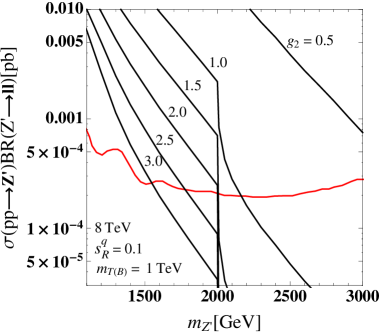
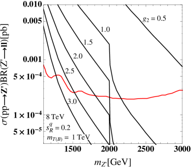
Figure 1: $\sigma(pp\to Z^{\prime})Br(Z^{\prime}\to\ell^{+}\ell^{-})$ as a function of $m_{Z^{\prime}}$ at $\sqrt{s}=8$ TeV with various values of $g_{2}$ for $s^{q}_{R}=0.1$ (left) and $s^{q}_{R}=0.2$ (right), where the masses of VLQs are fixed to be 1 TeV and the dashed red line shows the upper limit from the ATLAS experiment Aad:2014cka .

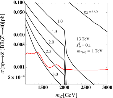
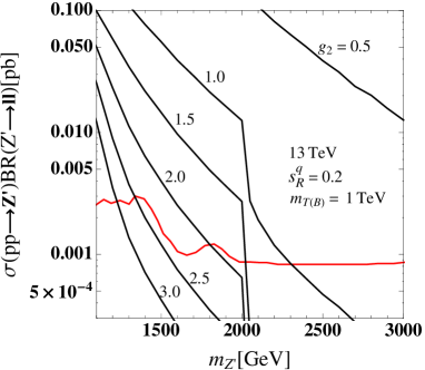
Figure 2: The legend is the same as that in Fig. 1 but for $\sqrt{s}=13$ TeV, where the experimental bound is from the ATLAS measurements ATLAS:dilepton .

III.2 Diphoton heavy Higgs boson decay

With the allowed $g_{2}$ and $m_{Z^{\prime}}$, we now study the phenomenon of the $H$ decay to diphoton. Since $H$ is a colorless scalar, the production process is through ggF. Therefore, the effective interaction for $Hgg$ induced from the VLQ loops is formulated as:

$${\cal L}_{ggH}=-\frac{\alpha_{s}}{8\pi}\left(\frac{n_{F}\sin\phi c_{R}^{q}y_{F}}{2\sqrt{2}m_{F}}A_{1/2}(\tau)\right)HG^{a\mu\nu}G^{a}_{\mu\nu}\,,$$ (75)

where $n_{F}=2$ is the number of VLQs and the loop function is:

$$A_{1/2}(\tau)=-2\tau[1+(1-\tau)f(\tau)^{2}]$$ (76)

with $\tau=4m_{F}^{2}/m_{H}^{2}$ and $f(x)=\sin^{-1}(1/\sqrt{x})$. Using Eq. (75), we can directly calculate the $H$ production cross section. Since we take $m_{F,H_{S}}>m_{H}$ and $\lambda_{12},\lambda_{1S},\mu_{1S}/m_{S}\ll 1$, the main $H$ decays are $H\to gg,\gamma\gamma,Z\gamma$. Although $H$ decay to $t$- and $b$-quark is allowed, due to the suppression of flavor mixings and $m_{t(b)}/m_{F}$, the associated BRs are much smaller than that of the diphoton decay. As such, we concentrate on the decays $H\to gg,\gamma\gamma,Z\gamma$ in the calculations.

From Eq. (75), the partial decay width for $H\to gg$ is derived as:

$$\Gamma(H\rightarrow gg)=\frac{\alpha_{s}^{2}m_{H}^{3}}{32\pi^{3}}\left|\frac{n_{F}\sin\phi c^{q}_{R}y_{F}}{2\sqrt{2}m_{F}}A_{1/2}(\tau)\right|^{2}\,.$$ (77)

It can be seen that $\Gamma(H\to gg)$ strongly depends on the $y_{F}$, $\sin\phi$, $m_{F}$, and flavor mixing $s^{q}_{R}$. In addition to the VLQ loops, the $W^{\prime}$-loop also contributes to $H\to\gamma\gamma$. The partial decay width for $H\to\gamma\gamma$ can be expressed as:

$$\Gamma(H\to\gamma\gamma)=\frac{\alpha^{2}m^{3}_{H}}{256\pi^{3}}\left|-\frac{y_{F}\sin\phi c_{R}^{q}Q^{2}_{{\rm em}}N_{c}}{\sqrt{2}m_{F}}A_{1/2}(\tau)+\frac{g_{2}\cos\phi}{2m_{W^{\prime}}}A_{1}(\xi)\right|^{2}\,,$$ (78)

where $N_{c}=3$ is the number of colors, $Q^{2}_{{\rm em}}=5/9$ is the sum of electric charge squares of $T$ and $B$ quarks, and $\xi=4m_{W^{\prime}}^{2}/m_{H}^{2}$. The loop function for the $W^{\prime}$-gauge boson is given by:

$$A_{1}(\xi)=2+3\xi+3\xi(2-\xi)f(\xi)^{2}.$$ (79)

Since the $W^{\prime}$ contribution in Eq. (78) is suppressed by $m_{W}^{\prime}$, $H\to gg$ is the dominant decay mode. Due to $\Gamma(H\to gg)\gg\Gamma(H\to\gamma\gamma)$ and $\Gamma(H\to Z\gamma)\approx\Gamma(H\to\gamma\gamma)$, we do not show up the detailed formula for $\Gamma(H\to Z\gamma)$, however, we include its numerical value when calculating the width. Although $H\to ZZ$ decay is allowed in our model, due to $\Gamma(H\to ZZ)\ll\Gamma(H\to\gamma\gamma)$, we ignore its contribution.

Since the $H$ production is dominated by the ggF channel, the diphoton production cross section at the center-of-energy of $\sqrt{s}$ in the narrow width approximation can be expressed as Franceschini:2015kwy :

$$\sigma(gg\to H\to\gamma\gamma)\approx\frac{C_{gg}}{s}\frac{\Gamma_{gg}}{m_{H}}{\cal B}_{\gamma\gamma}\,,$$ (80)

where $C_{gg}$ is related to the gluon luminosity function, $\Gamma_{gg}\equiv\Gamma(H\to gg)$, and ${\cal B}_{\gamma\gamma}\equiv BR(H\to\gamma\gamma)$ is the BR for the decay $H\to\gamma\gamma$. In order to perform the numerical analysis, we adopt $C_{gg}\approx 2137$ at $\sqrt{s}=13$ TeV and the K-factor for gluon fusion production process as $K_{gg}\simeq 1.5$ Franceschini:2015kwy . For comparison with the current upper bound on the diphoton resonance, we take the ATLAS data with $1\sigma$ errors and $m_{H}=750$ GeV ATLAS:2016eeo as:

$$\sigma(gg\to H\to\gamma\gamma)\leq 1.2\,{\rm fb}\,.$$ (81)

We now present the numerical analysis for $pp\to H\to\gamma\gamma$ by choosing some benchmark values of the free parameters. As mentioned earlier, the $H$ production and decays are sensitive to $y_{F}$, $m_{F}$, and $\sin\phi$. In order to display the dependence of these parameters, we present the contours for $\sigma(pp\to H\to\gamma\gamma)$ at $\sqrt{s}=13$ TeV as a function of $y_{F}$ and $m_{F}$ in Fig. 3(a), where the dashed lines with numbers on them are the cross section in units of fb, and we set $s^{q}_{R}=0.3$, $\sin\phi=1/\sqrt{2}$, and $g_{2}=3.3$. The parameter space in gray region has been excluded by the current ATLAS data as shown in Eq. (81). In addition, Fig. 3(b) shows the contours for the cross section as a function of $y_{F}$ and $\sin\phi$, where $s^{q}_{R}=0.3$, $m_{F}=1$ TeV, and $g_{2}=3.3$ are used. From the results, it can be seen that the Yukawa coupling with $y_{F}>1$ is limited by the current data. Other parameter region can be tested when more data are accumulated at the LHC.

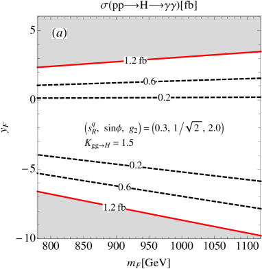
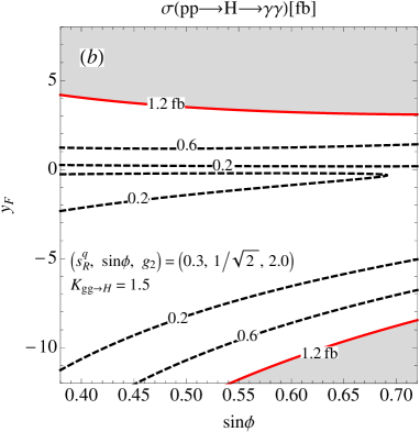
Figure 3: Contours for $\sigma(pp\to H\to\gamma\gamma)$ (dashed) as a function of (a) $y_{F}$ and $m_{F}$ (b) $y_{F}$ and $\sin\phi$, where the taken values of other parameters are shown in the plots. The gray region is excluded by the current ATLAS data.

III.3 Collider signatures of the model

We now study the possible collider signatures implied in the model. It is known that the masses of $W^{\prime}$ and $Z^{\prime}$ have to be heavier than 1.7 TeV. The production of $W^{\prime}/Z^{\prime}$ pairs is highly suppressed. For VLQ-pair production, it is found that the $\sigma(pp\to\bar{B}B/\bar{T}T)$ at $\sqrt{s}=13$ TeV is around 10-80 fb when $800\leq m_{F}\leq 1100$ GeV. With $m_{H}<m_{F}<m_{W^{\prime}/Z^{\prime}}$, the BRs for VLQ decays are $BR(T\to tH(h))=0.86(0.14)$ and $BR(B\to bH)\approx 1$. If we require that one $H$ decays to diphoton and the other decays to gluon-jet, by using the results in Fig. 3, the cross section for $pp\to\bar{Q}^{\prime}Q^{\prime}\to\bar{q}q(\gamma\gamma)_{H}(gg)_{H}$ is around 0.05-0.4 fb, where $Q^{\prime}=T(B)$ and $q=t(b)$.

Next, we study the single production of a new particle. Since $W^{\prime\pm}$ couple to the SM fermions via the flavor mixings, the production cross section for $W^{\prime}(t,b)$ is of order of $10^{-2}$ fb. The $Z^{\prime}$-boson can couple to the SM fermions without flavor mixing, however, the production cross section for $Z^{\prime}(t,b,\rm jet)$ is not large and is of order of $3$ fb. Although the VLQs can be as light as a few hundred GeV, the single $T(B)$-quark production is highly suppressed. We find that the production cross section for the process $pp\to H+{\rm jet}$ can reach 0.2 pb, where the dominant interaction is from $ggH$ shown in Eq. (75) and the associated Feynman diagram is sketched in Fig. 4. This channel can be used to further probe the scalar resonance. To show the detection possibility, we calculate the production cross section for $pp\to(\gamma\gamma)_{H}+{\rm jet}$ as a function of $m_{F}$ in Fig. 5(a), where the solid lines are for $y_{F}=-8,-6$, the dashed line is the SM result, the center of energy is $\sqrt{s}=13$ TeV, and the values of the parameters are set to be $\sin\phi=1/\sqrt{2}$, $g_{2}=2$, and $s^{q}_{R}=0.3$. In order to suppress the contributions from the SM, we adopt the following kinematic cuts:

$$P_{T}(\rm jet)\geq 150\ {\rm GeV}\,,~{}~{}P_{T}(\gamma)\geq 300\ {\rm GeV}\,,$$ (82)

where $P_{T}$ denotes the transverse momentum of a particle or a jet. It can be seen that $\sigma(pp\to(\gamma\gamma)_{H}+{\rm jet})$ in our model can be larger than $\sigma^{\rm SM}(pp\to\gamma\gamma+{\rm jet})$ after the kinematical cuts. For clarity, we also show the corresponding significance, which is defined by $S/\sqrt{B}$, in Fig. 5(b), where we have fixed $y_{F}=-8$ and the different lines are associated with different luminosities. It can be found that with a luminosity of $60$ fb^-1, the significance can be above $4\sigma$ for $m_{F}<900$ GeV.

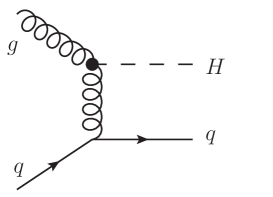
Figure 4: Feynman diagram for $pp\to H+$jet process where black dot indicates effective coupling in Eq. (75).

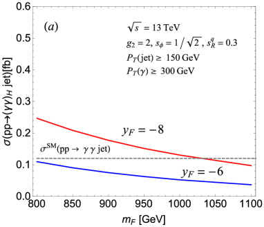
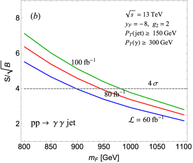
Figure 5: (a) Production cross section for $pp\to(\gamma\gamma)_{H}$ jet as a function of $m_{F}$, where the dashed line is the result from the SM, the solid lines are for $y_{F}=-8,\,-6$, and we adopt the kinematic cuts $P_{T}(\rm jet)\geq 150$ GeV and $P_{T}(\gamma)\geq 300$ GeV to suppress the background. (b) The corresponding significance of plot (a) with $y_{F}=-8$ and different luminosities.

IV Summary

The minimal renormalizable gauge theory that provides a new charged gauge boson is a local $SU(2)$ gauge symmetry. Thus, it is of interest to study the model with $SU(2)_{1}\times SU(2)_{2}\times U(1)_{Y}$ gauge symmetry. The $SU(2)_{2}$ gauge symmetry can be spontaneously broken by a $SU(2)_{2}$ doublet $H_{2}$. To avoid the complicated gauge anomaly cancellation, we consider an $SU(2)_{2}$ vector-like quark doublet $Q^{\prime}$ so that the charged gauge boson $W^{\prime}$ can decay into the vector-like quarks and SM quarks, and the production cross section and decay branching ratios of the heavy Higgs boson $H$ of $H_{2}$ can be enhanced.

It is found that to satisfy the precision $\rho$-parameter measurement, the masses of new gauge bosons have to be heavier than 1.7 TeV; the upper limits of the current dilepton resonance experiments can give a strict bound on the new gauge coupling $g_{2}$; and the bound of $g_{2}$ from $\rho$-parameter becomes stronger when $g_{2}>2$.

We add a scalar singlet $S$ in the model so that the $H$ boson can be produced via the gluon-gluon fusion channel due to the mixing effect between $S$ and $H$. It is found that the $W^{\prime}$ gauge boson plays an important role in the $H$ to diphoton decay. As a result, the production cross section for $pp\to H\to\gamma\gamma$ can reach the upper limits of the ATLAS and CMS experiments. To illustrate the interesting collider signature, we study the process $pp\to\gamma\gamma+{\rm jet}$ and its significances with various luminosities. By taking proper values of Yukawa coupling $y_{F}$ and mass of vector-like quark, the significance can easily be over $4\sigma$. In addition, other possible signatures to illustrate the new physics effects in our model are the production of vector-like quarks via $pp\to(\bar{T}T,\bar{B}B)$, in which the dominant decay modes are $T\to tH$ and $B\to bH$. We found that the production cross section can reach $0.4$ fb for $pp\to\bar{Q}^{\prime}Q^{\prime}\to\bar{q}q(\gamma\gamma)_{H}[\bar{q}q(gg)_{H}]$, which can be tested at the LHC.

Acknowledgments

The work of CHC was supported by the Ministry of Science and Technology of Taiwan, R.O.C., under grant MOST-103-2112-M-006-004-MY3.

References

- (1) G. Aad et al. [ATLAS Collaboration], JHEP 1512, 055 (2015) [arXiv:1506.00962 [hep-ex]].
- (2) V. Khachatryan et al. [CMS Collaboration], JHEP 1408, 173 (2014) [arXiv:1405.1994 [hep-ex]]; V. Khachatryan et al. [CMS Collaboration], JHEP 1408, 174 (2014) [arXiv:1405.3447 [hep-ex]]; V. Khachatryan et al. [CMS Collaboration], Phys. Lett. B 740, 83 (2015) [arXiv:1407.3476 [hep-ex]].
- (3) V. Khachatryan et al. [CMS Collaboration], Phys. Lett. B 749, 337 (2015) [arXiv:1502.07400 [hep-ex]].
- (4) V. Khachatryan et al. [CMS Collaboration], Phys. Rev. Lett. 116, no. 7, 071801 (2016) [arXiv:1512.01224 [hep-ex]].
- (5) G. Aad et al. [ATLAS Collaboration], Phys. Lett. B 754, 302 (2016) [arXiv:1512.01530 [hep-ex]].
- (6) S. Chatrchyan et al. [CMS Collaboration], Phys. Lett. B 720, 63 (2013) [arXiv:1212.6175 [hep-ex]].
- (7) G. Aad et al. [ATLAS Collaboration], Phys. Rev. D 90, no. 5, 052005 (2014) [arXiv:1405.4123 [hep-ex]].
- (8) The ATLAS collaboration, ATLAS-CONF-2015-070.
- (9) The ATLAS collaboration, ATLAS-CONF-2015-081.
- (10) M. Aaboud et al. [ATLAS Collaboration], JHEP 1609, 001 (2016) [arXiv:1606.03833 [hep-ex]].
- (11) CMS Collaboration [CMS Collaboration], CMS-PAS-EXO-15-004.
- (12) V. Khachatryan et al. [CMS Collaboration], Phys. Rev. Lett. 117, no. 5, 051802 (2016) [arXiv:1606.04093 [hep-ex]].
- (13) The ATLAS collaboration [ATLAS Collaboration], ATLAS-CONF-2016-059.
- (14) V. Khachatryan et al. [CMS Collaboration], arXiv:1609.02507 [hep-ex].
- (15) K. Harigaya and Y. Nomura, Phys. Lett. B 754, 151 (2016) [arXiv:1512.04850 [hep-ph]].
- (16) M. Backovic, A. Mariotti and D. Redigolo, JHEP 1603, 157 (2016) [arXiv:1512.04917 [hep-ph]].
- (17) A. Angelescu, A. Djouadi and G. Moreau, Phys. Lett. B 756, 126 (2016) [arXiv:1512.04921 [hep-ph]].
- (18) Y. Nakai, R. Sato and K. Tobioka, Phys. Rev. Lett. 116, no. 15, 151802 (2016) [arXiv:1512.04924 [hep-ph]].
- (19) D. Buttazzo, A. Greljo and D. Marzocca, Eur. Phys. J. C 76, no. 3, 116 (2016) [arXiv:1512.04929 [hep-ph]].
- (20) S. Di Chiara, L. Marzola and M. Raidal, Phys. Rev. D 93, no. 9, 095018 (2016) [arXiv:1512.04939 [hep-ph]].
- (21) S. Knapen, T. Melia, M. Papucci and K. Zurek, Phys. Rev. D 93, no. 7, 075020 (2016) [arXiv:1512.04928 [hep-ph]].
- (22) A. Pilaftsis, Phys. Rev. D 93, no. 1, 015017 (2016) [arXiv:1512.04931 [hep-ph]].
- (23) R. Franceschini et al., JHEP 1603, 144 (2016) [arXiv:1512.04933 [hep-ph]].
- (24) J. Ellis, S. A. R. Ellis, J. Quevillon, V. Sanz and T. You, JHEP 1603, 176 (2016) [arXiv:1512.05327 [hep-ph]].
- (25) R. S. Gupta, S. Jager, Y. Kats, G. Perez and E. Stamou, arXiv:1512.05332 [hep-ph].
- (26) A. Kobakhidze, F. Wang, L. Wu, J. M. Yang and M. Zhang, Phys. Lett. B 757 (2016) 92 [arXiv:1512.05585 [hep-ph]].
- (27) A. Falkowski, O. Slone and T. Volansky, JHEP 1602, 152 (2016) [arXiv:1512.05777 [hep-ph]].
- (28) R. Benbrik, C. H. Chen and T. Nomura, Phys. Rev. D 93, no. 5, 055034 (2016) [arXiv:1512.06028 [hep-ph]].
- (29) F. Wang, L. Wu, J. M. Yang and M. Zhang, Phys. Lett. B 759 (2016) 191 [arXiv:1512.06715 [hep-ph]].
- (30) P. S. B. Dev and D. Teresi, arXiv:1512.07243 [hep-ph].
- (31) B. C. Allanach, P. S. B. Dev, S. A. Renner and K. Sakurai, Phys. Rev. D 93, no. 11, 115022 (2016) [arXiv:1512.07645 [hep-ph]].
- (32) F. Wang, W. Wang, L. Wu, J. M. Yang and M. Zhang, arXiv:1512.08434 [hep-ph].
- (33) C. W. Chiang, M. Ibe and T. T. Yanagida, JHEP 1605, 084 (2016) [arXiv:1512.08895 [hep-ph]].
- (34) R. Martinez, F. Ochoa and C. F. Sierra, arXiv:1512.05617 [hep-ph].
- (35) W. Chao, arXiv:1512.06297 [hep-ph].
- (36) S. Chang, Phys. Rev. D 93, no. 5, 055016 (2016) [arXiv:1512.06426 [hep-ph]].
- (37) T. F. Feng, X. Q. Li, H. B. Zhang and S. M. Zhao, arXiv:1512.06696 [hep-ph].
- (38) S. M. Boucenna, S. Morisi and A. Vicente, arXiv:1512.06878 [hep-ph].
- (39) A. E. C. Hernandez and I. Nisandzic, arXiv:1512.07165 [hep-ph].
- (40) U. Kumar Dey, S. Mohanty and G. Tomar, Phys. Lett. B 756, 384 (2016) [arXiv:1512.07212 [hep-ph]].
- (41) G. M. Pelaggi, A. Strumia and E. Vigiani, JHEP 1603, 025 (2016) [arXiv:1512.07225 [hep-ph]].
- (42) J. de Blas, J. Santiago and R. Vega-Morales, arXiv:1512.07229 [hep-ph].
- (43) W. C. Huang, Y. L. S. Tsai and T. C. Yuan, arXiv:1512.07268 [hep-ph].
- (44) K. M. Patel and P. Sharma, arXiv:1512.07468 [hep-ph].
- (45) K. Das and S. K. Rai, arXiv:1512.07789 [hep-ph].
- (46) J. Cao, L. Shang, W. Su, F. Wang and Y. Zhang, arXiv:1512.08392 [hep-ph].
- (47) Q. H. Cao, Y. Liu, K. P. Xie, B. Yan and D. M. Zhang, arXiv:1512.08441 [hep-ph].
- (48) P. S. B. Dev, R. N. Mohapatra and Y. Zhang, JHEP 1602, 186 (2016) [arXiv:1512.08507 [hep-ph]].
- (49) Y. Jiang, Y. Y. Li and T. Liu, arXiv:1512.09127 [hep-ph].
- (50) A. Dasgupta, M. Mitra and D. Borah, arXiv:1512.09202 [hep-ph].
- (51) P. Ko, Y. Omura and C. Yu, arXiv:1601.00586 [hep-ph].
- (52) A. Karozas, S. F. King, G. K. Leontaris and A. K. Meadowcroft, arXiv:1601.00640 [hep-ph].
- (53) T. Modak, S. Sadhukhan and R. Srivastava, Phys. Lett. B 756, 405 (2016) [arXiv:1601.00836 [hep-ph]].
- (54) B. Dutta, Y. Gao, T. Ghosh, I. Gogoladze, T. Li, Q. Shafi and J. W. Walker, arXiv:1601.00866 [hep-ph].
- (55) F. F. Deppisch, C. Hati, S. Patra, P. Pritimita and U. Sarkar, arXiv:1601.00952 [hep-ph].
- (56) A. Berlin, Phys. Rev. D 93, no. 5, 055015 (2016) [arXiv:1601.01381 [hep-ph]].
- (57) D. Borah, S. Patra and S. Sahoo, arXiv:1601.01828 [hep-ph].
- (58) P. Ko and T. Nomura, Phys. Lett. B 758, 205 (2016) [arXiv:1601.02490 [hep-ph]].
- (59) C. Hati, Phys. Rev. D 93, no. 7, 075002 (2016) [arXiv:1601.02457 [hep-ph]].
- (60) J. H. Yu, arXiv:1601.02609 [hep-ph].
- (61) I. Dorsner, S. Fajfer and N. Kosnik, arXiv:1601.03267 [hep-ph].
- (62) A. E. Faraggi and J. Rizos, Eur. Phys. J. C 76, no. 3, 170 (2016) [arXiv:1601.03604 [hep-ph]].
- (63) U. Aydemir and T. Mandal, arXiv:1601.06761 [hep-ph].
- (64) F. Staub et al., arXiv:1602.05581 [hep-ph].
- (65) P. Ko, T. Nomura, H. Okada and Y. Orikasa, arXiv:1602.07214 [hep-ph].
- (66) J. Ren and J. H. Yu, arXiv:1602.07708 [hep-ph].
- (67) G. Lazarides and Q. Shafi, arXiv:1602.07866 [hep-ph].
- (68) U. Aydemir, D. Minic, C. Sun and T. Takeuchi, arXiv:1603.01756 [hep-ph].
- (69) D. T. Huong and P. V. Dong, Phys. Rev. D 93, no. 9, 095019 (2016) [arXiv:1603.05146 [hep-ph]].
- (70) G. K. Leontaris and Q. Shafi, arXiv:1603.06962 [hep-ph].
- (71) C. Kownacki and E. Ma, arXiv:1604.01148 [hep-ph].
- (72) H. P. Nilles and M. W. Winkler, JHEP 1605, 182 (2016) [arXiv:1604.03598 [hep-ph]].
- (73) M. Duerr, P. Fileviez Perez and J. Smirnov, arXiv:1604.05319 [hep-ph].
- (74) F. Takahashi, M. Yamada and N. Yokozaki, arXiv:1604.07145 [hep-ph].
- (75) B. Dutta, Y. Gao, T. Ghosh, I. Gogoladze, T. Li and J. W. Walker, arXiv:1604.07838 [hep-ph].
- (76) H. Davoudiasl, P. P. Giardino and C. Zhang, arXiv:1605.00037 [hep-ph].
- (77) The ATLAS collaboration [ATLAS Collaboration], ATLAS-CONF-2016-059.
- (78) V. Khachatryan et al. [CMS Collaboration], arXiv:1609.02507 [hep-ex].
- (79) J. L. Hewett and T. G. Rizzo, Phys. Rept. 183, 193 (1989).
- (80) P. Langacker, Rev. Mod. Phys. 81, 1199 (2009) [arXiv:0801.1345 [hep-ph]].
- (81) E. Salvioni, G. Villadoro and F. Zwirner, JHEP 0911, 068 (2009) [arXiv:0909.1320 [hep-ph]].
- (82) M. S. Chanowitz, Phys. Rev. D 84, 035014 (2011) [arXiv:1102.3672 [hep-ph]].
- (83) R. N. Mohapatra and J. C. Pati, Phys. Rev. D 11, 566 (1975); Phys. Rev. D 11, 2558 (1975).
- (84) G. Senjanovic and R. N. Mohapatra, Phys. Rev. D 12, 1502 (1975).
- (85) P. Langacker and S. U. Sankar, Phys. Rev. D 40, 1569 (1989).
- (86) T. G. Rizzo, JHEP 0705, 037 (2007) doi:10.1088/1126-6708/2007/05/037 [arXiv:0704.0235 [hep-ph]].
- (87) M. Schmaltz and C. Spethmann, JHEP 1107, 046 (2011) [arXiv:1011.5918 [hep-ph]].
- (88) J. F. Gunion, H. E. Haber, G. L. Kane and S. Dawson, Front. Phys. 80, 1 (2000).
- (89) G. Aad et al. [ATLAS Collaboration], Eur. Phys. J. C 76, no. 1, 6 (2016) [arXiv:1507.04548 [hep-ex]].
- (90) G. Aad et al. [ATLAS and CMS Collaborations], JHEP 1608, 045 (2016) [arXiv:1606.02266 [hep-ex]].
- (91) K.A. Olive et al. (Particle Data Group), Chin. Phys. C, 38, 090001 (2014).
- (92) A. Belyaev, N. D. Christensen and A. Pukhov, Comput. Phys. Commun. 184, 1729 (2013) [arXiv:1207.6082 [hep-ph]].
- (93) P. M. Nadolsky, H. L. Lai, Q. H. Cao, J. Huston, J. Pumplin, D. Stump, W. K. Tung and C.-P. Yuan, Phys. Rev. D 78, 013004 (2008) [arXiv:0802.0007 [hep-ph]].