Long-range entangled zero-mode state in a non-Hermitian lattice

Abstract

In contrast to a Hermitian system, in which zero modes are usually degenerate and localized edge state in the thermodynamic limit, the zero mode of a finite non-Hermitian system can be a single nontrivial long-range entangled state at the exceptional point (EP). In this work, we demonstrate this feature with a concrete example based on exact solutions. Numerical simulations show that the entangled state can be generated through the dynamic process with a high fidelity.

I Introduction

Non-Hermitian systems make many things possible including quantum phase transition occurred in a finite system Znojil1 ; Znojil2 ; Bendix ; LonghiPRL ; LonghiPRB1 ; Jin1 ; Znojil3 ; LonghiPRB2 ; LonghiPRB3 ; Jin2 ; Joglekar1 ; Znojil4 ; Znojil5 ; Zhong ; Drissi ; Joglekar2 ; Scott1 ; Joglekar3 ; Scott2 ; Tony , unidirectional propagation and anomalous transport LonghiPRL ; Kulishov ; LonghiOL ; Lin ; Regensburger ; Eichelkraut ; Feng ; Peng ; Chang , invisible defects LonghiPRA2010 ; Della ; ZXZ , coherent absorption Sun and self sustained emission Mostafazadeh ; LonghiSUS ; ZXZSUS ; Longhi2015 ; LXQ , loss-induced revival of lasing PengScience , as well as laser-mode selection FengScience ; Hodaei . Such kinds of novel phenomena can be traced to the existence of exceptional or spectral singularity points. Exploring novel quantum states in non-Hermitian systems becomes an attractive topic. It is well known that a midgap state must be a localized state without the long-range correlation. Two degenerate edge states can always construct two long-range correlated states. However, it is hard to generate a single long-range correlated state in practice due to the degeneracy. On the other hand, a prepared state is fragile due to the interaction with the environment. A gap protected long-range correlated state is desirable in many fields. For instance, in quantum information science, it is a crucial problem to develop techniques for generating entanglement among stationary qubits, which play a central role in applications Ekert ; Deutsch ; Bennett .

In this paper, we consider whether it is possible to find a midgap state with nontrivial long-range correlation in a non-Hermitian system. We revisit the system of a tight-binding chain with two conjugated imaginary potentials at the end sites, which has received many studies Bendix ; Jin1 ; Joglekar1 ; Joglekar2 ; Joglekar3 ; Longhi2013 ; Ganainy ; Makris ; Guo ; Ruter ; Regensburger ; ChenS . Based on the exact results, we show that there exists a single zero-mode state with long-range correlation. This system acts as a double well potential, which has two spatial modes (see Fig. 1). We propose a scheme to generate a midgap entangled state through the dynamic process in a finite non-Hermitian system. Numerical simulations show that the entangled zero-mode state can be achieved with a high fidelity via the time evolution of an easily prepared initial state.

The remainder of this paper is organized as follows. In Sec. II, we present a non-Hermitian chain and zero-mode solutions. Sec. III reveals the implication of the zero-mode solution. Sec. IV demonstrates the mode entanglement in the zero-mode state. Sec. V devotes to the scheme for the generation of long-range entanglement. Finally, we present a summary and discussion in Sec. VI.

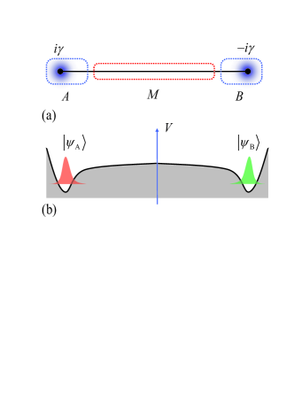
Figure 1: (color online). Schematics for a dimerized chain with two end imaginary potentials as a quantum entangler. (a) The whole chain is decomposed into three parts. A and B are both $N_{0}$-site, $M$ is $N-2N_{0}$ site. At exceptional point (EP), there is a single zero-mode state, which is an approximately maximal entangled state for the spatial modes of parties A and B. (b) Schematic illustration of the zero-mode state. The chain system acts as a double well potential, which has two spatial modes $\left|\psi_{\mathrm{A}}\right\rangle$ and $\left|\psi_{\mathrm{B}}\right\rangle$. The zero-mode state is similar to the ground state of the potential well, being an entangled state of the two spatial modes.

II Model and coalescing zero-mode

We consider a non-Hermitian model with complex boundary potentials and its Hamiltonian is

$$H = H_{0}+H_{\gamma},$$

$$H_{0} = -\kappa\sum_{j=1}^{N/2}a_{2j-1}^{\dagger}a_{2j}-\sum_{j=1}^{N/2-1}a_{2j}^{\dagger}a_{2j+1}+\mathrm{H.c.,}$$ (1)

$$H_{\gamma} = i\gamma a_{1}^{\dagger}a_{1}-i\gamma a_{N}^{\dagger}a_{N},$$

where $a_{l}^{{\dagger}}$ is the creation operator of the boson (or fermion) at $l$th site. There are two sets of hopping integrals with strength $\kappa$ and $1$, respectively. For simplicity, we only consider the case with $N/2=$ even. The Hamiltonian $H$ has $\mathcal{PT}$ symmetry, i.e., $[H,\mathcal{PT}]=0$, where $\mathcal{P}$ and $\mathcal{T}$ represent the space-reflection operator, or parity operator and the time-reversal operator, respectively. The effects of $\mathcal{P}$ and $\mathcal{T}$ on a discrete system are

$$\mathcal{T}i\mathcal{T}=-i\text{, }\mathcal{P}a_{l}^{{\dagger}}\mathcal{P}=a_{N+1-l}^{{\dagger}}.$$ (2)

Since the discovery of Bender and colleagues in 1998 that a non-Hermitian Hamiltonian having simultaneous parity-time $\mathcal{PT}$ symmetry has an entirely real quantum-mechanical energy spectrum Bender , there has been an intense effort to establish a $\mathcal{PT}$-symmetric quantum theory as a complex extension of the conventional quantum mechanics. The reality of the spectra is responsible to the $\mathcal{PT}$ symmetry. If all the eigenstates of the Hamiltonian are also eigenstates of $\mathcal{PT}$, then all the eigenvalues are strictly real and the symmetry is said to be unbroken. Otherwise, the symmetry is said to be spontaneously broken. On the other hand, the unitary time-evolution of wave functions in a non-Hermitian Hamiltonian could also be guaranteed when redefining the biorthogonal inner product instead of the Dirac inner product. However, when the system is under the EP, the norm of biorthogonal inner product for coalescing eigenstates is zero.

In the case of $\kappa=1$, it has been shown in Ref. Jin1 that this model exhibits two phases, an unbroken symmetry phase with a purely real energy spectrum when the potentials are in the region $\gamma<1$ and a spontaneously-broken symmetry phase with $N-2$ real and $2$ imaginary eigenvalues when the potentials are in the region $\gamma>1$. The EP occurs at $\gamma=1$, at which two zero-energy eigenstates coalesce. In the case of $\kappa\neq 1$, the model is systematically investigated in Ref. ChenS .

In this work, we revisit this model from another perspective, focusing on the property of coalescing zero-mode state based on exact solutions. We start with the case of $\gamma=0$ and $0<\kappa<1$. According to bulk-boundary correspondence, there are two zero modes at the middle of the band gap for infinite $N$, characterizing the topology of the band Ryu ; Ganeshan . These two states are all called edge modes, since they are localized states, with the particle probability distributing at the ends of the chain. For finite $N$, two zero modes split near the zero energy. We are interested in what happens when the imaginary potentials $\pm i\gamma$ are switched on. It is a little bit complicated to get and analyze the exact solutions. Numerical simulation shows that the EP occurs at a certain value of $\gamma$, at which the two midgap states coalesce to a single eigenstate. Fortunately, we can demonstrate this point by a simple exact result.

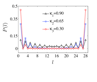
Figure 2: (color online). Profiles of the Dirac probability distribution of the zero-mode states for systems at their corresponding EPs. We consider an $N=28$ chain with typical values of $\kappa$ with critical $\gamma_{\mathrm{c}}=\kappa^{N/2}$, respectively.

A straightforward derivation shows that when taking

$$\gamma=\gamma_{\mathrm{c}}=\kappa^{N/2},$$ (3)

the state defined as $\left|\psi_{\mathrm{zm}}\right\rangle=\psi_{\mathrm{zm}}^{{\dagger}}\left|\text{{Vac}}\right\rangle$ is a zero-mode eigenstate, where state $\left|\text{{Vac}}\right\rangle$ is defined as

$$\left|\text{{Vac}}\right\rangle=\prod_{j=1}^{N}\left|0\right\rangle_{j},$$ (4)

and $\left|0\right\rangle_{j}$ is the vacuum state of particle operator $a_{j}^{\dagger}$, i.e., $a_{j}\left|0\right\rangle_{j}=0$. And field operator is

$$\psi_{\mathrm{zm}}^{{\dagger}}=\Omega\sum_{j=1}^{N/2}[\left(-\kappa\right)^{j-1}a_{2j-1}^{\dagger}-i\left(-\kappa\right)^{N/2-j}a_{2j}^{\dagger}],$$ (5)

i.e.,

$$H\left(\gamma_{\mathrm{c}}\right)\left|\psi_{\mathrm{zm}}\right\rangle=0.$$ (6)

Furthermore, the many-particle state $(\psi_{\mathrm{zm}}^{{\dagger}})^{n}\left|\text{{Vac}}\right\rangle$ is still a zero-mode eigenstate. Here $\Omega=\sqrt{\left(1-\kappa^{2}\right)/\left(2-2\kappa^{N}\right)}$ is the Dirac normalizing constant. Similarly, the zero-mode state for $H_{\gamma_{\mathrm{c}}}^{\dagger}$ can be constructed as

$$\left|\eta_{\mathrm{zm}}\right\rangle=\Omega\sum_{j=1}^{N/2}[\left(-\kappa\right)^{j-1}a_{2j-1}^{\dagger}+i\left(-\kappa\right)^{N/2-j}a_{2j}^{\dagger}]\left|\text{{Vac}}\right\rangle,$$ (7)

satisfying

$$[H\left(\gamma_{\mathrm{c}}\right)]^{\dagger}\left|\eta_{\mathrm{zm}}\right\rangle=0.$$ (8)

On the other hand, it is easy to check

$$\left\langle\eta_{\mathrm{zm}}\right.\left|\psi_{\mathrm{zm}}\right\rangle=0,$$ (9)

and

Figure 3: (color online). Schematics for the Hermitian correspondence of the zero-mode state. (a) $\mathcal{PT}$ symmetric non-Hermitian chain, (b) $\mathcal{P}$ symmetric Hermitian ring. When the on-site imaginary potentials $\pm i\gamma$ and the boundary hopping $\lambda$ satisfy the zero-mode conditions in Eq. (3) and (13), the two systems share a same zero-mode state.

$$\left|\eta_{\mathrm{zm}}\right\rangle=i\mathcal{P}\left|\psi_{\mathrm{zm}}\right\rangle,$$ (10)

which indicate that the coalescing levels typically produce not only eigenstates but also adjoint states. In the context of non-Hermitian quantum mechanics, the adjoint states refer to the eigenstates of $H^{{\dagger}}$, which always share the same spectrum with those of $H$. Both the eigenstates of $H$ and $H^{{\dagger}}$ could construct the biorthogonal inner product instead of the Dirac inner product in order to guarantee the unitary time-evolution of wave functions in a non-Hermitian Hamiltonian. When the system is under the EP, two eigenstates of $H$ coalesce and the norm of biorthogonal inner product for coalescing eigenstates is zero. Meanwhile, it is a natural result that two eigenstates of $H^{{\dagger}}$ also coalesce due to the fact $H^{{\dagger}}=H(\gamma\rightarrow-\gamma)$. Here the two coalescing eigenstates of $H$($H^{{\dagger}}$) would become only one eigenstate in the non-Hermitian system while there are two-fold degenerate states in the Hermitian system that we will consider in the next section. The existence of two-fold degenerate entangled states in the Hermitian system would degrade the efficiency of the entangled state in practice. While, there is a single midgap entangled state in the non-Hermitian system, which is robust.

Based on these facts we conclude that the zero-mode state $\left|\psi_{\mathrm{zm}}\right\rangle$ is a coalescing state and the EP occurs at $\gamma_{\mathrm{c}}$. The exact wave function of $\left|\psi_{\mathrm{zm}}\right\rangle$ clearly indicates that it is a superposition of two parts with nonzero amplitudes only located at even or odd sites, respectively. It will be shown that such two parts, which consist of even and odd sites respectively, have a close relation to the standard edge states of a Hermitian chain in the thermodynamic limit.

In our work, we explore the quantum correlation, entanglement of a midgap state for a non-Hermitian Hamiltonian. Unlike the dynamics, such the feature of a state has no memory about its own history. One cannot detect how the state was prepared, via a Hermitian or non-Hermitian system. In contrast, the metric of biorthogonal inner product in non-Hermitian quantum mechanics is dependent of Hamiltonian. Meanwhile, when the system is under the EP, the norm of biorthogonal inner product for coalescing eigenstates is zero, which is the characteristic of a non-Hermitian system. On the other hand, the entanglement is measured via local Dirac probability in experiments. In Fig. 2, we plot the profiles of the Dirac probability distribution of the zero-mode states in a $28$-site chain at EPs where all the zero-mode states have been normalized in Dirac inner product. Here the local Dirac probability is defined as $P\left(l\right)=\left|\left\langle l\right.\left|\psi_{\mathrm{zm}}\right\rangle\right|^{2}$ with $\left|l\right\rangle=a_{l}^{\dagger}\left|\mathrm{Vac}\right\rangle$. We see that a smaller $\kappa$ requires a smaller $\gamma_{\mathrm{c}}$, leading to more localized probability distribution and bigger gap. It is the key feature of the non-Hermitian zero-mode state, which should have wild applications in many aspects. We will demonstrate this point explicitly in the following sections.

III Hermitian correspondence for zero-mode state

In this section, we investigate the property of the zero-mode state. We consider a Hermitian model on the same lattice with $H$ and its Hamiltonian is

$$H_{\mathrm{hc}} = H_{0}+H_{\lambda},$$ (11)

$$H_{\lambda} = -\lambda a_{1}^{\dagger}a_{N}+\mathrm{H.c.}.$$ (12)

The Hamiltonian $H_{\mathrm{hc}}$ has $\mathcal{P}$ symmetry, i.e., $[H_{\mathrm{hc}},\mathcal{P}]=0$. Then all the eigenstates should have reflection symmetry. We still investigate the midgap state through a simple exact solution. In Fig. 3, the two systems $H$ and $H_{\mathrm{hc}}$ are schematically illustrated.

A straightforward derivation shows that when taking

$$\lambda=\lambda_{\mathrm{c}}=\kappa^{N/2},$$ (13)

the state is defined as $\left|\psi_{\sigma}\right\rangle=\psi_{\sigma}^{{\dagger}}\left|\text{{Vac}}\right\rangle$ with $\sigma=\pm$, and

$$\psi_{\pm}^{{\dagger}}=\Omega\sum_{j=1}^{N/2}[\left(-\kappa\right)^{j-1}a_{2j-1}^{\dagger}\pm i\left(-\kappa\right)^{N/2-j}a_{2j}^{\dagger}],$$ (14)

is the field operator of zero-mode eigenstate, i.e.,

$$H\left(\lambda_{\mathrm{c}}\right)\left|\psi_{\pm}\right\rangle=0.$$ (15)

It is easy to find that

$$\left|\psi_{\mathrm{zm}}\right\rangle=\left|\psi_{-}\right\rangle,\left|\eta_{\mathrm{zm}}\right\rangle=\left|\psi_{+}\right\rangle.$$ (16)

The relation between zero-mode states of the non-Hermitian Hamiltonian $H$ and the Hermitian one $H_{\mathrm{hc}}$ is very clear, that is, the two Hamiltonians share a same zero-mode state.

Furthermore, one can obtain the exact wave function for the standard zero modes by simply taking $N\rightarrow\infty$, i.e., $\lambda_{\mathrm{c}}=\lim_{N\rightarrow\infty}\kappa^{N/2}=0$. Then our Hermitian model would become a standard SSH chain and accordingly the standard edge states can be defined as $\left|\psi_{Y}\right\rangle=\psi_{Y}^{{\dagger}}\left|\text{{Vac}}\right\rangle$ with $Y=L$, $R$, where

$$\psi_{\mathrm{L}}^{{\dagger}} = \sqrt{2}\Omega\sum_{j=1}^{\infty}\left(-\kappa\right)^{j-1}a_{2j-1}^{\dagger},$$ (17)

$$\psi_{\mathrm{R}}^{{\dagger}} = \sqrt{2}\Omega\sum_{j=1}^{\infty}\left(-\kappa\right)^{N/2-j}a_{2j}^{\dagger},$$ (18)

with $\left|\psi_{\mathrm{L}}\right\rangle=\lim_{N\rightarrow\infty}\left(\left|\psi_{+}\right\rangle+\left|\psi_{-}\right\rangle\right)/\sqrt{2}$ and $\left|\psi_{\mathrm{R}}\right\rangle=-i\lim_{N\rightarrow\infty}\left(\left|\psi_{+}\right\rangle-\left|\psi_{-}\right\rangle\right)/\sqrt{2}$.

Interestingly, one can see that the profile of the wave functions are unchanged. Then we get the conclusion that wave functions $\left|\psi_{\mathrm{zm}}\right\rangle$, $\left|\eta_{\mathrm{zm}}\right\rangle,$ and $\left|\psi_{\pm}\right\rangle$, can be obtained directly by the truncations of the standard zero-mode wave functions.

It appears an interesting “coincidence” that the zero-mode states in Eq. (14) are identical to those of the non-Hermitian Hamiltonian. Here we would like to give a further explanation on the essential of the “coincidence”. We note that in both Hermitian and non-Hermitian lattices, the sub-Hamiltonians in the region far from the boundary are identical, i.e.,

$$H_{\mathrm{mid}}=-\kappa\sum_{j}a_{2j-1}^{\dagger}a_{2j}-\sum_{j}a_{2j}^{\dagger}a_{2j+1}+\mathrm{H.c.}.$$ (19)

And in this region the single-particle wave function can be expressed as

$$\left|\psi_{k}\right\rangle = \sum_{j}(A_{k}e^{ikj}+B_{k}e^{-ikj})a_{2j-1}^{\dagger}\left|\text{{Vac}}\right\rangle$$ (20)

$$+\sum_{j}(C_{k}e^{ikj}+D_{k}e^{-ikj})a_{2j}^{\dagger}\left|\text{{Vac}}\right\rangle,$$

where $A_{k}$, $B_{k}$, $C_{k}$, and $D_{k}$ are undetermined parameters. Then the corresponding Schrodinger equation for a zero-mode state has the forms

$$\left\{\begin{array}[]{c}-\kappa(A_{k}e^{ikj}+B_{k}e^{-ikj})-\left[A_{k}e^{ik\left(j+1\right)}+B_{k}e^{-ik\left(j+1\right)}\right]=0,\\ -\kappa(C_{k}e^{ikj}+D_{k}e^{-ikj})-\left[C_{k}e^{ik\left(j-1\right)}+D_{k}e^{-ik\left(j-1\right)}\right]=0,\end{array}\right.$$ (21)

which lead to

$$\left\{\begin{array}[]{c}\left(\kappa+e^{ik}\right)A_{k}e^{ikj}+\left(\kappa+e^{-ik}\right)B_{k}e^{-ikj}=0,\\ \left(\kappa+e^{-ik}\right)C_{k}e^{ikj}+\left(\kappa+e^{ik}\right)D_{k}e^{-ikj}=0,\end{array}\right.$$ (22)

or the compact form

$$\left(\begin{array}[]{cccc}h_{11}&0&0&0\\ 0&h_{22}&0&0\\ 0&0&h_{33}&0\\ 0&0&0&h_{44}\end{array}\right)\left(\begin{array}[]{c}A_{k}\\ B_{k}\\ C_{k}\\ D_{k}\end{array}\right)=0,$$ (23)

with

$$h_{11} = h_{44}=\kappa+e^{ik},$$ (24)

$$h_{22} = h_{33}=\kappa+e^{-ik}.$$ (25)

The existence of the solution requires that

$$\det\left(\begin{array}[]{cccc}h_{11}&0&0&0\\ 0&h_{22}&0&0\\ 0&0&h_{33}&0\\ 0&0&0&h_{44}\end{array}\right)=0,$$ (26)

or

$$\left(\kappa+e^{ik}\right)\left(\kappa+e^{-ik}\right)=0.$$ (27)

In our work, we only consider the case with $0<\kappa<1$. Then the possible solution of $k$ is

$$k=\pi-i\ln\kappa\text{ or }k=\pi+i\ln\kappa,$$ (28)

which describes an evanescent wave in accord with the edge state at the midgap.

This fact indicates that both Hermitian and non-Hermitian systems share a common $k$ and therefore the main form of their wave functions is similar. The parameters $A_{k}$, $B_{k}$, $C_{k}$, and $D_{k}$ or the relations between them could be finally determined by the boundary and normalization conditions. Based on the above analysis, we could achieve two degenerate solutions for the Hermitian system, while only one solution for the non-Hermitian system (for the zero-mode state of $H^{\dagger}$, we can only follow the same method above after taking $\gamma\rightarrow-\gamma$ due to the reason $H^{{\dagger}}=H(\gamma\rightarrow-\gamma)$). In this sense, the “coincidence” becomes natural if suitable boundary conditions for the two systems are chosen.

IV Mode entanglement

Entanglement is an intriguing characteristic of quantum mechanics and is fundamentally different from any correlation known in classical physics. It would be interesting for both quantum information and condensed matter if one could generate particular entangled states in a controlled manner. The typical entanglement refers to a two-particle system. However, it has been demonstrated that the mode entanglement of a single particle can be used for dense coding and quantum teleportation despite the superselection rule Heaney . In the following, we study the mode entanglement in the zero-mode state.

First of all, we define two spacial-mode states $\left|\psi_{\mathrm{A}}\right\rangle=\psi_{\mathrm{A}}^{{\dagger}}\left|\text{{Vac}}\right\rangle$ and $\left|\psi_{\mathrm{B}}\right\rangle=\psi_{\mathrm{B}}^{{\dagger}}\left|\text{{Vac}}\right\rangle$, i.e.,

$$\left|\psi_{\mathrm{A}}\right\rangle = \Omega_{0}\sum_{j=1}^{N_{0}/2}\left(-\kappa\right)^{j-1}a_{2j-1}^{\dagger}\left|\text{{Vac}}\right\rangle,$$ (29)

$$\left|\psi_{\mathrm{B}}\right\rangle = -i\Omega_{0}\sum_{j=N_{\mathrm{B}}}^{N/2}\left(-\kappa\right)^{N/2-j}a_{2j}^{\dagger}\left|\text{{Vac}}\right\rangle,$$ (30)

where $\Omega_{0}=\sqrt{\left(1-\kappa^{2}\right)/\left(1-\kappa^{N_{0}}\right)}$ is the Dirac normalizing constant and $N_{\mathrm{B}}=\left(N-N_{0}+2\right)/2$. $\psi_{X}^{{\dagger}}$ is the field operator for spatial mode $X=A$, $B$, i.e., $\psi_{\mathrm{A}}^{{\dagger}}\left|\text{{Vac}}\right\rangle=\left|1\right\rangle_{\mathrm{A}}\left|0\right\rangle_{\mathrm{B}}$ and $\psi_{\mathrm{B}}^{{\dagger}}\left|\text{{Vac}}\right\rangle=\left|0\right\rangle_{\mathrm{A}}\left|1\right\rangle_{\mathrm{B}}$. Here

$$\left|1\right\rangle_{\mathrm{A}} = \psi_{\mathrm{A}}^{{\dagger}}\left|0\right\rangle_{\mathrm{A}},\left|1\right\rangle_{\mathrm{B}}=\psi_{\mathrm{B}}^{{\dagger}}\left|0\right\rangle_{\mathrm{B}},$$ (31)

$$\left|0\right\rangle_{\mathrm{A}} = \prod_{j=1}^{N/2}\left|0\right\rangle_{2j-1},\left|0\right\rangle_{\mathrm{B}}=\prod_{j=1}^{N/2}\left|0\right\rangle_{2j}.$$ (32)

And the spacial mode states defined in Eqs. (29) and (30) are introduced to characterize the entanglement feature of the zero-mode states, the formalism of which is adopted and studied in Ref. Heaney . And these two spacial mode states could construct a target entangled state $(\left|\psi_{\mathrm{A}}\right\rangle+\left|\psi_{\mathrm{B}}\right\rangle)/\sqrt{2}=(\left|1\right\rangle_{\mathrm{A}}\left|0\right\rangle_{\mathrm{B}}+\left|0\right\rangle_{\mathrm{A}}\left|1\right\rangle_{\mathrm{B}})/\sqrt{2}$, which can be used to judge the degree of entanglement of the zero-mode state of $H$.

Taking $N_{0}=N$, the zero-mode state can be written as

$$\left|\psi_{\mathrm{zm}}\right\rangle=\frac{1}{\sqrt{2}}(\left|1\right\rangle_{\mathrm{A}}\left|0\right\rangle_{\mathrm{B}}+\left|0\right\rangle_{\mathrm{A}}\left|1\right\rangle_{\mathrm{B}})$$ (33)

which is a maximal entanglement. When we measure the state of the subsystem $A$ $(B)$, it will collapse to either $\left|1\right\rangle_{\mathrm{A}}\left|0\right\rangle_{\mathrm{B}}$ or $\left|0\right\rangle_{\mathrm{A}}\left|1\right\rangle_{\mathrm{B}}$, i.e., when $\left|\psi_{\mathrm{A}}\right\rangle$ is detected at $A$, party $B$ must collapse to empty state $\left|0\right\rangle_{\mathrm{B}}$. However, such an entangled state is not useful for teleportation in quantum information processing, since the particle probability may not distribute locally.

An interesting fact is that, for $N_{0}\ll N$, but small $\kappa$, we still have

$$\left|\psi_{\mathrm{zm}}\right\rangle\approx\frac{1}{\sqrt{2}}(\left|1\right\rangle_{\mathrm{A}}\left|0\right\rangle_{\mathrm{B}}+\left|0\right\rangle_{\mathrm{A}}\left|1\right\rangle_{\mathrm{B}}),$$ (34)

i.e., the zero-mode state is a highly entangled state for the localized spacial-mode states.

And here we introduce the quantity

$$\mathcal{F}(N,N_{0},\kappa)=\left|\left\langle\psi_{\mathrm{zm}}\right|\frac{\left|1\right\rangle_{\mathrm{A}}\left|0\right\rangle_{\mathrm{B}}+\left|0\right\rangle_{\mathrm{A}}\left|1\right\rangle_{\mathrm{B}}}{\sqrt{2}}\right|,$$ (35)

to characterize the entanglement of a zero-mode state for the situation with parameters $N$, $N_{0}$, and $\kappa$. A simple derivation yields

$$\mathcal{F}(N,N_{0},\kappa)=\sqrt{\frac{1-\kappa^{N_{0}}}{1-\kappa^{N}}},$$ (36)

which is close to $\sqrt{1-\kappa^{N_{0}}}$ for $N\gg N_{0}$. It indicates that a system with $\kappa^{N_{0}}\ll 1$ can achieve a perfect entangled state.

V Generation of entanglement

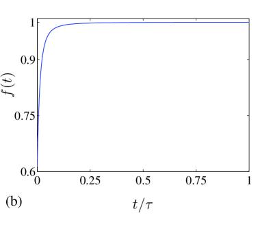
Figure 4: (color online). Dynamical process for the generation of the entangled zero-mode state. (a) The probability distributions $P(l,t)$ for several instants are obtained by the time evolution of the simplest initial state $\left|1\right\rangle$ under the Hamiltonian $H$ with $N=28$, $\kappa=0.5$, and $\gamma=\gamma_{\mathrm{c}}+10^{-10}$. Here the red dot indicates the probability distribution of the zero-mode state. (b) Plot of the fidelity as a function of time with $\tau=8\times 10^{5}.$

Entanglement naturally exists in the zero-mode state, which is protected by the band gap. The question in practice is how to create such a state. Recently, generation scheme of several typical entangled states has been proposed by the dynamical process near the EP of non-Hermitian systems Tony1 ; Tony2 ; LC . The key to the scheme is based on the fact that a pseudo-Hermitian system has real eigenvalues or conjugate pair complex eigenvalues Bender ; Ann ; JMP1 ; JPA1 ; PRL1 ; JMP2 ; JPA3 ; JPA5 . Considering the situation in this work that the single zero-mode state splits to a pair of eigenstates with conjugate complex eigenvalues and the $\mathcal{PT}$ symmetry of those eigenstates have been broken, when we tune the potential to $\gamma=\gamma_{\mathrm{c}}+0^{+}$. This pair of states are very close to the zero-mode state, in the sense of that they are still long-range entangled states. A seed state is an initial state consisting of various eigenstates with their eigenvalues including zero, positive, and negative imaginary parts, respectively. As time evolution, the amplitude of the state with positive imaginary part among the eigenvalues will increase exponentially and suppress that of other components. The target is the final steady state, which can be regarded as the zero-mode state in the point of view of Dirac product.

The initial state is taken as $\left|\psi\left(0\right)\right\rangle=\left|1\right\rangle$, and the evolved state $\left|\psi\left(t\right)\right\rangle$ is expected to close to the target state $\left|\psi_{\mathrm{zm}}\right\rangle$ for a sufficient long time. Whether the Hamiltonian operator $H$ is Hermitian or not, an evolved vector $\left|\psi\left(t\right)\right\rangle$ should always be the solution of the Schrodinger equation

$$i\frac{\partial}{\partial t}\left|\psi\left(t\right)\right\rangle=H\left|\psi\left(t\right)\right\rangle.$$ (37)

And the solution has the form

$$\left|\psi\left(t\right)\right\rangle=e^{-iHt}\left|\psi\left(0\right)\right\rangle,$$ (38)

which can be computed by using a uniform mesh in the time discretization for method. Of course, by taking the biorthogonal inner product instead of the Dirac inner product in order to guarantee the unitary time-evolution of the wave functions in a non-Hermitian Hamiltonian, one can also compute the time evolution by expanding the initial state in terms of the complete set of biorthonormal energy eigenstates. We employ the fidelity

$$f\left(t\right)=\left|\left\langle\psi_{\mathrm{zm}}\right|\widetilde{\psi}\left(t\right)\rangle\right|,$$ (39)

to characterize the efficiency of the scheme. Here $\left|\widetilde{\psi}\left(t\right)\right\rangle$ is the Dirac normalized state of $\left|\psi\left(t\right)\right\rangle$ to reduce the increasing norm of $\left|\psi\left(t\right)\right\rangle$. In order to quantitatively evaluate the fidelity and demonstrate the proposed scheme, we simulate the dynamic process of the state $\left|\psi_{\mathrm{zm}}\right\rangle$ preparation. We plot the profiles of $\left|\widetilde{\psi}\left(t\right)\right\rangle$ at several typical instants and the fidelity $f\left(t\right)$ in Fig. 4. We see that the perfect edge state $\left|1\right\rangle$ spreads out rapidly at the beginning and converges to the target state with a high fidelity after a long time.

VI Summary

In conclusion, we have studied the midgap zero-mode state in a non-Hermitian discrete system. The exact result for a dimerized tight-binding chain with two end imaginary potentials substantiates the existence of coalescing zero-mode state. Based on the exact results, it is found that, the zero-mode state exhibits robust long-range spatial mode entanglement, which is not achievable in a Hermitian system. We have also investigated the entanglement generation scheme. Numerical simulations indicate that such a midgap state can be generated by the time evolution of an easily prepared initial state. Our finding extends the understanding of non-Hermitian quantum mechanics and should have wide applications in quantum engineering.

- (1) M. Znojil, Phys. Lett. B 650, 440 (2007).
- (2) M. Znojil, J. Phys. A 40, 13131 (2007).
- (3) O. Bendix, R. Fleischmann, T. Kottos, and B. Shapiro, Phys. Rev. Lett. 103, 030402 (2009).
- (4) S. Longhi, Phys. Rev. Lett. 103, 123601 (2009).
- (5) S. Longhi, Phys. Rev. B 80, 235102 (2009).
- (6) L. Jin and Z. Song, Phys. Rev. A 80, 052107 (2009).
- (7) M. Znojil, Phys. Rev. A 82, 052113 (2010).
- (8) S. Longhi, Phys. Rev. B 81, 195118 (2010).
- (9) S. Longhi, Phys. Rev. B 82, 041106(R) (2010).
- (10) L. Jin and Z. Song, Phys. Rev. A 81, 032109 (2010).
- (11) Y. N. Joglekar, D. Scott, M. Babbey, and A. Saxena, Phys. Rev. A 82, 030103(R) (2010).
- (12) M. Znojil, J. Phys. A 44, 075302 (2011).
- (13) M. Znojil, Phys. Lett. A 375, 2503 (2011).
- (14) H. Zhong, W. Hai, G. Lu, and Z. Li, Phys. Rev. A 84, 013410 (2011).
- (15) L. B. Drissi, E. H. Saidi, and M. Bousmina, J. Math. Phys. 52, 022306 (2011).
- (16) Y. N. Joglekar and A. Saxena, Phys. Rev. A 83, 050101(R) (2011).
- (17) D. D. Scott and Y. N. Joglekar, Phys. Rev. A 83, 050102(R) (2011).
- (18) Y. N. Joglekar and J. L. Barnett, Phys. Rev. A 84, 024103 (2011).
- (19) D. D. Scott and Y. N. Joglekar, Phys. Rev. A 85, 062105 (2012).
- (20) T. E. Lee and Y. N. Joglekar, Phys. Rev. A 92, 042103 (2015).
- (21) M. Kulishov et al, Opt. Express 13, 3068 (2005).
- (22) S. Longhi, Opt. Lett. 35, 3844 (2010).
- (23) Z. Lin, H. Ramezani, T. Eichelkraut, T. Kottos, H. Cao, and D. N. Christodoulides, Phys. Rev. Lett. 106, 213901 (2011).
- (24) A. Regensburger, C. Bersch, M. Ali Miri, G. Onishchukov, D. N. Christodoulides, and U. Peschel, Nature (London) 488, 167 (2012).
- (25) T. Eichelkraut et al, Nat. Commun. 4, 2533 (2013).
- (26) L. Feng et al, Nat. Mater. 12, 108 (2013).
- (27) B. Peng et al, Nat. Phys. 10, 394 (2014).
- (28) L. Chang, Nat. Photonics 8, 524 (2014).
- (29) S. Longhi, Phys. Rev. A 82, 032111 (2010).
- (30) S. Longhi and G. Della Valle, Ann. Phys. (NY) 334, 35 (2013).
- (31) X. Z. Zhang and Z. Song, Ann. Phys. (NY) 339, 109 (2013).
- (32) Y. Sun, W. Tan, H. Q. Li, J. Li, and H. Chen, Phys. Rev. Lett. 112, 143903 (2014).
- (33) A. Mostafazadeh, Phys. Rev. Lett. 102, 220402 (2009).
- (34) S. Longhi, Phys. Rev. B 80, 165125 (2009).
- (35) X. Z. Zhang, L. Jin, and Z. Song, Phys. Rev. A 87, 042118 (2013).
- (36) S. Longhi, Opt. Lett. 40, 5694 (2015).
- (37) X. Q. Li, X. Z. Zhang, G. Zhang, and Z. Song, Phys. Rev. A 91, 032101 (2015).
- (38) B. Peng et al, Science 346, 328 (2014).
- (39) L. Feng, Z. J. Wong, R. -M. Ma, Y. Wang, and X. Zhang, Science 346, 972 (2014).
- (40) H. Hodaei, M. -A. Miri, M. Heinrich, D. N. Christodoulides, and M. Khajavikhan, Science 346, 975 (2014).
- (41) A. K. Ekert, Phys. Rev. Lett. 67, 661 (1991).
- (42) D. Deutsch and R. Jozsa, Proc. R. Soc. London A 439, 553 (1992).
- (43) C. H. Bennett, G. Brassard, C. Crepeau, R. Jozsa, A. Peres, and W. K. Wootters, Phys. Rev. Lett. 70, 1895 (1993).
- (44) S. Longhi, Phys. Rev. A 88, 052102 (2013).
- (45) R. El-Ganainy, K. G. Makris, D. N. Christodoulides, and Z. H. Musslimani, Opt. Lett. 32, 2632 (2007).
- (46) K. G. Makris, R. El-Ganainy, D. N. Christodoulides, and Z. H. Musslimani, Phys. Rev. Lett. 100, 103904 (2008).
- (47) A. Guo, G. J. Salamo, D. Duchesne, R. Morandotti, M. Volatier-Ravat, V. Aimez, G. A. Siviloglou, and D. N. Christodoulides, Phys. Rev. Lett. 103, 093902 (2009).
- (48) C. E. Ruter, K. G. Makris, R. El-Ganainy, D. N. Christodoulides, M. Segev, and D. Kip, Nat. Phys. 6, 192 (2010).
- (49) B. G. Zhu, R. Lu, and S. Chen, Phys. Rev. A 89, 062102 (2014).
- (50) C. M. Bender and S. Boettcher, Phys. Rev. Lett. 80, 5243 (1998).
- (51) S. Ryu and Y. Hatsugai, Phys. Rev. Lett. 89, 077002 (2002).
- (52) S. Ganeshan, K. Sun, and S. Das Sarma, Phys. Rev. Lett. 110, 180403 (2013).
- (53) L. Heaney and V. Vedral, Phys. Rev. Lett. 103, 200502 (2009).
- (54) T. E. Lee, F. Reiter, and N. Moiseyev, Phys. Rev. Lett. 113, 250401 (2014).
- (55) T. E. Lee and C. K. Chan, Phys. Rev. X 4, 041001 (2014).
- (56) C. Li and Z. Song, Phys. Rev. A 91, 062104 (2015).
- (57) F. G. Scholtz, H. B. Geyer, and F. J. W. Hahne, Ann. Phys. (NY) 213, 74 (1992).
- (58) C. M. Bender, S. Boettcher, and P. N. Meisinger, J. Math. Phys. 40, 2201 (1999).
- (59) C. M. Bender, D. C. Brody, and H. F. Jones, Phys. Rev. Lett. 89, 270401 (2002).
- (60) P. Dorey, C. Dunning, and R. Tateo, J. Phys. A 34, L391 (2001); ibid. 34, 5679 (2001).
- (61) A. Mostafazadeh, J. Math. Phys. 43, 205 (2002); ibid. 43, 2814 (2002); ibid. 43, 3944 (2002).
- (62) A. Mostafazadeh and A. Batal, J. Phys. A 36, 7081 (2003); ibid. 37, 11645 (2004).
- (63) H. F. Jones, J. Phys. A 38, 1741 (2005).