An analytic family of post-merger template waveforms

Abstract

Building on the analytical description of the post-merger (ringdown) waveform of coalescing, non-precessing, spinning, (BBHs) introduced in Phys. Rev. D 90, 024054 (2014), we propose an analytic, closed form, time-domain, representation of the $\ell=m=2$ gravitational radiation mode emitted after merger. This expression is given as a function of the component masses and dimensionless spins $(m_{1,2},\chi_{1,2})$ of the two inspiralling objects, as well as of the mass $M_{\rm BH}$ and (complex) frequency $\sigma_{1}$ of the fundamental quasi-normal mode of the remnant black hole. Our proposed template is obtained by fitting the post-merger waveform part of several publicly available numerical relativity simulations from the Simulating eXtreme Spacetimes (SXS) catalog and then suitably interpolating over (symmetric) mass ratio and spins. We show that this analytic expression accurately reproduces ($\sim$ 0.01 rad) the phasing of the post-merger data of other datasets not used in its construction. This is notably the case of the spin-aligned run SXS:BBH:0305, whose intrinsic parameters are consistent with the 90% credible intervals reported by the parameter-estimation followup of GW150914 in Phys. Rev. Lett. 116 (2016) no.24, 241102. Using SXS waveforms as “experimental” data, we further show that our template could be used on the actual GW150914 data to perform a new measure the complex frequency of the fundamental quasi-normal mode so to exploit the complete (high signal-to-noise-ratio) post-merger waveform. We assess the usefulness of our proposed template by analysing, in a realistic setting, SXS full inspiral-merger-ringdown waveforms and constructing posterior probability distribution functions for the central frequency damping time of the first overtone of the fundamental quasi-normal mode as well as for the physical parameters of the systems. We also briefly explore the possibility opened by our waveform model to test the second law of black hole dynamics. Our model will help improve current tests of general relativity, in particular the general-relativistic no-hair theorem, and allow for novel tests, such as that of the area theorem.

I Introduction

One of the most difficult challenges provided by the discovery of GW150914 Abbott et al. (2016a) is to find robust evidence that the system is made by two black holes that eventually coalesce into a final black hole according to the predictions of general relativity (GR). An avenue pursued in  Abbott et al. (2016b) is to show consistency between the early-inspiral and the late-inspiral parts of the gravitational wave signal, with this latter, according to GR, dominated by the quasi-normal mode (QNM) frequencies of the final black hole. This nontrivial issue was carefully addressed in Ref. Abbott et al. (2016b), that followed the discovery paper Abbott et al. (2016a). In addition to the global waveform consistency test, Ref. Abbott et al. (2016b) looked for evidence of the existence of the fundamental QNM in the post-merger signal. Ref. Abbott et al. (2016b) fit the signal at time $t>t_{0}$, with $t_{0}$ an arbitrary time after the merger time, $t_{\rm M}$, with a simple exponentially-damped oscillatory template of the form $Ae^{-\alpha(t-t_{0})}\cos[2\pi f_{0}(t-t_{0})+\phi_{0}]$. With this method, it was found that the 90% posterior contour starts overlapping the GR prediction at $t_{0}=t_{\rm M}+3~{}{\rm ms}$, i.e. approximately $10M$ after the merger point (see Fig. 4 in Abbott et al. (2016b)). At later times, where theory predicts the fundamental QNM frequency to be persistent and dominant, the signal-to-noise-ratio (SNR) becomes too small, the statistical uncertainty becomes large and the signal is undetectable around $t_{0}\geq t_{\rm M}+8$ ms.

The direct measurement of the frequency and damping time of the fundamental QNM of the final black hole provides the most convincing evidence that the observed event is fully consistent with a binary black hole coalescence to a final single black hole as predicted by GR. However, due to the nature of the fitting template mentioned above, there are about $10M$ of signal, approximately corresponding to half a gravitational-wave (GW) cycle, which contributes significantly to the SNR, whose physical content is unexploited for the aforementioned analysis. Hence, the conclusions of Ref. Abbott et al. (2016b) could be further strengthened by a reliable, analytical model, in the time-domain, of the complete post-merger part of the waveform (where the “merger” is defined as the peak of the $|{\cal R}h_{22}|$ waveform) to be used as a fitting template. This would allow for more flexibility in performing the analysis, that is currently limited, due to the particular choice of the fitting template, to just the late-time (low SNR) part of the signal, where among all QNMs (that get excited at the moment of merger), only the least-damped fundamental one is still present. This paper introduces a novel waveform template, in the time-domain, designed to describe the complete post-merger signal, with the long term goal to improve the post-merger analysis of GW150914 of Ref. Abbott et al. (2016b) and similar signals that will likely be detected in the future by the LIGO and Virgo Collaborations. This template is based upon the analytical representation of the post-merger waveform for coalescing, non-precessing, BBH of Ref. Damour and Nagar (2014a). This representation is obtained by interpolation of the primary fits of the post-merger numerical relativity (NR) waveform part after that the first, least-damped, QNM is factored out. The primary fit effectively models the presence of all the higher QNMs, that are characterized by lower frequencies and shorter damping times than the fundamental one. Ref. Damour and Nagar (2014a) focused on the equal-mass, equal-spin case only and thus used only the corresponding subset of the Simulating eXtreme Spacetimes (SXS) sxs catalog of numerical waveform data. All SXS waveforms were obtained with the Spectral Einstein Code Chu et al. (2009); Mroue and Pfeiffer (2012); Hemberger et al. (2013); Lovelace et al. (2011, 2012); Buchman et al. (2012); Mroue et al. (2013); Scheel et al. (2015). We generalize here the interpolating expressions of Ref. Damour and Nagar (2014a), by including several of the unequal-mass, unequal-spin dataset present in the SXS catalog, i.e. the waveform previously used for EOB/NR information and comparison in Ref. Nagar et al. (2016) plus a few more that were publicly available in June 2016, when the first draft of this study was conceived, but we do not include the dataset added to the catalog on October 31st, 2016 (see below). We thus build a general analytical expression of the post-merger waveform that is a function of the symmetric mass ratio $\nu\equiv m_{1}m_{2}/(m_{1}+m_{2})^{2}$ and of the dimensionless spins $\chi_{1,2}\equiv S_{1,2}/(m_{1,2})^{2}$ of the two black holes as well as of the final mass $M_{\rm BH}$ and (complex) frequency $\sigma_{1}$ of the fundamental QNM of the final remnant. Although we restrict, for simplicity, to considering only the $\ell=m=2$ mode, the method discussed here may be extended to model the post-merger part of subdominant multipolar modes . The interpolating, improved, fit presented here is also now part of the NR-informed ${\tt EOB\_{ihes}}$ EOB code Nagar et al. (2016); Damour and Nagar (2014b).

The paper is organized as follows: In Sec. II we construct the analytic template waveform, while Sec. III is devoted to testing is accuracy and reliability. The performance of the template in a simulated data-analysis setup is evaluated in Sec. IV and we summarize our findings in Sec. V.

II Template construction

We begin by introducing a convenient notation. The multipolar decomposition of the waveform is given by $h_{+}-{\rm i}h_{\times}=\sum_{\ell,m}h_{\ell m}{}_{-2}Y_{\ell m}(\theta,\phi)$, and we focus on the $\ell=m=2$ “post-merger”, $\nu$-scaled, waveform,

$$h(\tau)\equiv\dfrac{1}{\nu}\dfrac{{\cal R}c^{2}}{GM}h_{22}^{\rm postmerger}(\tau),$$ (1)

where $M\equiv m_{1}+m_{2}$ is the total mass and ${\cal R}$ is the distance of the source. The time $\tau=(t-t_{\rm M})/M_{\rm BH}$ counts time in units of the mass of the final black hole, $M_{\rm BH}$, and $t_{\rm M}$ is the merger time. The QNM-rescaled ringdown waveform $\bar{h}(\tau)$ of Damour and Nagar (2014a) $h(\tau)$ is defined as $h(\tau)\equiv e^{-\sigma_{1}\tau-{\rm i}\phi_{0}}\bar{h}(\tau)$, where $\sigma_{1}\equiv\alpha_{1}+{\rm i}\omega_{1}$ is the (dimensionless, $M_{\rm BH}$-rescaled) complex frequency of the fundamental (positive frequency, $\omega_{1}>0$) QNM of the final black hole and $\phi_{0}$ is the value of the phase at merger. The (complex) function $\bar{h}(\tau)$ is then decomposed in amplitude and phase as

$$\bar{h}(\tau)\equiv A_{\bar{h}}e^{{\rm i}\phi_{{\bar{h}}}(\tau)}.$$ (2)

Reference Damour and Nagar (2014a) found that $A_{{\bar{h}}}$ and $\phi_{{\bar{h}}}$ can be accurately represented by the following general functional forms

$$A_{\bar{h}}(\tau) =c_{1}^{A}{\rm tanh}(c_{2}^{A}\tau+c_{3}^{A})+c^{A}_{4},$$ (3)

$$\phi_{\bar{h}}(\tau) =-c_{1}^{\phi}\ln\left(\dfrac{1+c_{3}^{\phi}e^{-c_{2}^{\phi}\tau}+c_{4}^{\phi}e^{-2c_{2}^{\phi}\tau}}{1+c_{3}^{\phi}+c_{4}^{\phi}}\right).$$ (4)

Table 1: The $\nu$-dependence of the coefficients in Eq. (10).

$A_{\alpha_{21}}=$	$-0.0185533\,\nu$	$-0.0166417$
$B_{\alpha_{21}}=$	$-0.0594092\,\nu$	$-0.0157896$
$C_{\alpha_{21}}=$	$-0.100191\,\nu$	$+0.19044$
$A_{\alpha_{1}}=$	$-0.0123998\,\nu$	$-0.00791069$
$B_{\alpha_{1}}=$	$-0.0421559\,\nu$	$-0.00365094$
$C_{\alpha_{1}}=$	$-0.040671\,\nu$	$+0.0919055$
$A_{c_{3}^{A}}=$	$+0.417778\,\nu$	$-0.0175206$
$B_{c_{3}^{A}}=$	$+0.0243799\,\nu$	$-0.22621$
$C_{c_{3}^{A}}=$	$+0.953089\,\nu$	$-0.592121$
$A_{c_{3}^{\phi}}=$	$+12.9727\,\nu$	$-0.350191$
$B_{c_{3}^{\phi}}=$	$-0.249142\,\nu$	$+3.10091$
$C_{c_{3}^{\phi}}=$	$-1.6901\,\nu$	$+4.44107$
$A_{c_{4}^{\phi}}=$	$+23.3553\,\nu$	$+1.9222$
$B_{c_{4}^{\phi}}=$	$-0.448352\,\nu$	$+4.99249$
$C_{c_{4}^{\phi}}=$	$-3.05867\,\nu$	$+2.70508$
$A_{\Delta\omega}=$	$+0.129442\,\nu$	$+0.0232987$
$B_{\Delta\omega}=$	$+0.165507\,\nu$	$+0.0517482$
$C_{\Delta\omega}=$	$+0.383848\,\nu$	$+0.0850474$
$A_{\hat{A}_{22}^{\rm mrg}}=$	$+0.229867\,\nu$	$-0.0411679$
$B_{\hat{A}_{22}^{\rm mrg}}=$	$-0.450254\,\nu$	$+0.107428$
$C_{\hat{A}_{22}^{\rm mrg}}=$	$+0.742481\,\nu$	$+1.38748$
$A_{\omega_{22}^{\rm mrg}}=$	$-0.285624\,\nu$	$+0.0903558$
$B_{\omega_{22}^{\rm mrg}}=$	$-0.185274\,\nu$	$+0.12597$
$C_{\omega_{22}^{\rm mrg}}=$	$+0.405274\,\nu$	$+0.258643$

As in Ref. Damour and Nagar (2014a), only three of the eight fitting coefficients, $(c_{3}^{A},c_{3}^{\phi},c_{4}^{\phi})$, are independent and need to be fit directly. The others can be expressed in terms of four other physical quantities: ($\alpha_{1},\alpha_{21},\Delta\omega,\hat{A}_{22}^{\rm mrg}$)

$$c_{2}^{A} =\dfrac{1}{2}\alpha_{21},$$ (5)

$$c_{4}^{A} =\hat{A}_{22}^{\rm mrg}-c_{1}^{A}\tanh(c_{3}^{A}),$$ (6)

$$c_{1}^{A} =\hat{A}_{22}^{\rm mrg}\,\alpha_{1}\dfrac{\cosh^{2}(c_{3}^{A})}{c_{2}^{A}},$$ (7)

$$c_{1}^{\phi} =\Delta\omega\dfrac{1+c_{3}^{\phi}+c_{4}^{\phi}}{c_{2}^{\phi}(c_{3}^{\phi}+2c_{4}^{\phi})},$$ (8)

$$c_{2}^{\phi} =\alpha_{21},$$ (9)

Table 2: Dataset of the SXS catalog used for the cross-validation of the template waveform, see Fig. 3. The datasets marked with an * were used in the construction of the template. The dataset SXS:BBH:none is a 14 orbit waveform not part of the SXS catalog Buchman et al. (2012) that was used to calibrate EOB models Pan et al. (2011); Damour et al. (2013). From left to right, the columns report: the dataset number in the SXS catalog, the mass ratio $q=m_{1}/m_{2}$; the symmetric-mass ratio $\nu\equiv m_{1}m_{2}/(m_{1}+m_{2})^{2}$; the dimensionless spins; the mass and angular momentum of the final black hole $(M_{\rm BH},J_{\rm BH})$; the NR phase at merger time ($\tau=0$), $\phi_{0}^{\rm NR_{mrg}}$; and the corresponding GW frequency $M_{\rm BH}\omega_{22}^{\rm mrg}$. The value of $\phi_{0}^{\rm NR_{\rm mrg}}$ is used to align the NR and analytical waveforms at $\tau=0$ in Fig. 1.

ID	$q$	$\nu$	$S_{1}/(m_{1})^{2}$	$S_{2}/(m_{2})^{2}$	$M_{\rm BH}/M$	$J_{\rm BH}/M_{\rm BH}^{2}$	$\phi_{0}^{\rm NR_{mrg}}$	$M_{\rm BH}\omega_{22}^{\rm mrg}$
SXS:BBH:none*	1	$0.25$	$0$	$0$	0.95161	0.6864	$0.8579$	0.3422
SXS:BBH:0152*	1	$0.25$	$+0.60$	$+0.60$	0.9269	0.8578	$-2.7441$	0.3849
SXS:BBH:0211	1	$0.25$	$+0.90$	$-0.90$	0.9511	0.6835	$2.1415$	0.3415
SXS:BBH:0178*	1	$0.25$	$+0.994$	$+0.994$	0.8867	0.9499	$0.0856$	0.4199
SXS:BBH:0305	1.221	$0.2475$	$+0.33$	$-0.4399$	0.9520	0.6921	$2.6594$	0.3427
SXS:BBH:0025	1.5	$0.2400$	$+0.4995$	$-0.4995$	0.9504	0.7384	$-0.4623$	$0.3513$
SXS:BBH:0184	2	$0.\bar{2}$	$0$	0	0.9612	0.6234	$-3.0966$	0.3336
SXS:BBH:0162	2	$0.\bar{2}$	$+0.60$	$0$	0.9461	0.8082	$-1.6577$	0.3687
SXS:BBH:0257	2	$0.\bar{2}$	$+0.85$	$+0.85$	0.9199	0.9175	$2.2626$	0.4152
SXS:BBH:0045	3	$0.1875$	$+0.4995$	$-0.4995$	0.9628	0.7410	$-2.6842$	0.3617
SXS:BBH:0292	3	$0.1875$	$+0.7314$	$-0.8493$	0.9560	0.8266	$1.9684$	0.3750
SXS:BBH:0293	3	$0.1875$	$+0.85$	$+0.85$	0.9142	0.9362	$-2.6663$	$0.4158$
SXS:BBH:0317	3.327	$0.1777$	$0.5226$	$-0.4482$	0.9642	0.7462	$-0.3756$	0.3677
SXS:BBH:0208*	5	$0.13\bar{8}$	$-0.90$	0	0.98822	$-0.12817$	$+0.5148$	0.2626
SXS:BBH:0203	7	$0.1094$	$+0.40$	$0$	0.9836	$0.6056$	$-0.9013$	0.3341
SXS:BBH:0207	7	$0.1094$	$-0.60$	$0$	0.9909	$-0.0769$	$-1.3736$	0.2631
SXS:BBH:0064*	8	$0.0987$	$-0.50$	$0$	0.9922	$-0.0526$	$2.3926$	0.2634
SXS:BBH:0185	9.990	$0.0827$	$0$	$0$	0.9917	$0.2608$	$0.4982$	0.2948

Table 3: The last two columns list fundamental QNMs frequencies and final black hole mass inferred from NR data and measured with the post-merger template, after adding to the NR waveform white Gaussian noise. For all NR waveforms, the total mass is fixed to $M=60M_{\odot}$ and we consider postmerger SNR=10 and SNR=50. The uncertainty on the measured quantities corresponds to the $90\%$ credible regions. The measures of both $M_{\rm BH}$ and $\sigma_{1}$ are biased for some specific datasets with large mass ratio and spin anti-aligned with the orbital angular momentum.

ID	$(q,\chi_{1},\chi_{2})$	$\sigma_{1}^{\rm NR}$	$\sigma_{1}|_{\rm SNR=10}$	$M_{\rm BH}/M_{\odot}|_{\rm SNR=10}$	$\sigma_{1}|_{\rm SNR=50}$	$M_{\rm BH}/M_{\odot}|_{\rm SNR=50}$
SXS:BBH:none*	$(1,0,0)$	$0.0813+{\rm i}0.527$	$0.07_{-0.02}^{+0.03}+{\rm i}0.52_{-0.17}^{+0.19}$	$57.1_{-17.2}^{+19.6}$	$0.08_{-0.01}^{+0.01}+{\rm i}0.50_{-0.06}^{+0.06}$	$54.3_{-5.4}^{+5.4}$
SXS:BBH:0152*	$(1,+0.60,+0.60)$	$0.0706+{\rm i}0.629$	$0.07_{-0.03}^{+0.03}+{\rm i}0.78_{-0.31}^{+0.20}$	$69.5_{-27.2}^{+18.0}$	$0.08_{-0.01}^{+0.01}+{\rm i}0.67_{-0.11}^{+0.10}$	$59.0_{-8.6}^{+7.6}$
SXS:BBH:0211	$(1,-0.90,+0.90)$	$0.081+{\rm i}0.525$	$0.11_{-0.04}^{+0.04}+{\rm i}0.85_{-0.33}^{+0.14}$	$99.6_{-38.0}^{+17.7}$	$0.08_{-0.01}^{+0.02}+{\rm i}0.50_{-0.08}^{+0.09}$	$56.2_{-7.5}^{+8.6}$
SXS:BBH:0178*	$(1,+0.994,+0.994)$	$0.053+{\rm i}0.746$	$0.08_{-0.03}^{+0.04}+{\rm i}0.74_{-0.23}^{+0.22}$	$55.3_{-16.2}^{+17.1}$	$0.06_{-0.00}^{+0.01}+{\rm i}0.73_{-0.04}^{+0.05}$	$52.7_{-2.4}^{+3.1}$
SXS:BBH:0305	$(1.2,+0.33,-0.44)$	$0.081+{\rm i}0.529$	$0.11_{-0.05}^{+0.09}+{\rm i}0.88_{-0.33}^{+0.11}$	$92.4_{-34.3}^{+15.5}$	$0.10_{-0.03}^{+0.04}+{\rm i}0.62_{-0.18}^{+0.26}$	$65.7_{-17.6}^{+24.8}$
SXS:BBH:0025	$(1.5,+0.5,-0.5)$	$0.079+{\rm i}0.550$	$0.12_{-0.04}^{+0.06}+{\rm i}0.90_{-0.27}^{+0.09}$	$94.8_{-28.3}^{+13.1}$	$0.09_{-0.02}^{+0.02}+{\rm i}0.58_{-0.12}^{+0.14}$	$60.6_{-11.0}^{+12.7}$
SXS:BBH:0184	$(2,0,0)$	$0.083+{\rm i}0.502$	$0.26_{-0.22}^{+0.22}+{\rm i}0.54_{-0.41}^{+0.41}$	$39.0_{-28.2}^{+116.4}$	$0.13_{-0.06}^{+0.09}+{\rm i}0.85_{-0.34}^{+0.14}$	$97.8_{-40.1}^{+22.4}$
SXS:BBH:0162	$(2,+0.60,0)$	$0.075+{\rm i}0.591$	$0.11_{-0.06}^{+0.08}+{\rm i}0.74_{-0.35}^{+0.24}$	$77.5_{-37.1}^{+29.0}$	$0.07_{-0.01}^{+0.01}+{\rm i}0.59_{-0.09}^{+0.10}$	$56.4_{-7.5}^{+8.0}$
SXS:BBH:0257	$(2,+0.85,+0.85)$	$0.062+{\rm i}0.694$	$0.08_{-0.04}^{+0.05}+{\rm i}0.74_{-0.29}^{+0.23}$	$64.3_{-24.6}^{+21.6}$	$0.07_{-0.01}^{+0.01}+{\rm i}0.71_{-0.06}^{+0.06}$	$56.2_{-3.8}^{+4.1}$
SXS:BBH:0045	$(3,+0.5,-0.5)$	$0.079+{\rm i}0.552$	$0.31_{-0.23}^{+0.17}+{\rm i}0.53_{-0.40}^{+0.43}$	$131.1_{-86.2}^{+52.8}$	$0.14_{-0.05}^{+0.05}+{\rm i}0.88_{-0.29}^{+0.11}$	$89.9_{-28.7}^{+14.0}$
SXS:BBH:0292	$(3,+0.73,-0.85)$	$0.073+{\rm i}0.604$	$0.11_{-0.05}^{+0.05}+{\rm i}0.85_{-0.28}^{+0.14}$	$86.2_{-29.7}^{+17.9}$	$0.08_{-0.01}^{+0.01}+{\rm i}0.64_{-0.07}^{+0.08}$	$60.1_{-5.7}^{+6.1}$
SXS:BBH:0293	$(3,+0.85,+0.85)$	$0.062+{\rm i}0.689$	$0.09_{-0.03}^{+0.04}+{\rm i}0.86_{-0.26}^{+0.13}$	$74.2_{-22.0}^{+13.0}$	$0.08_{-0.01}^{+0.01}+{\rm i}0.77_{-0.09}^{+0.11}$	$62.6_{-6.0}^{+7.1}$
SXS:BBH:0317	$(3.3,0.52,-0.45)$	$0.078+{\rm i}0.554$	$0.08_{-0.04}^{+0.05}+{\rm i}0.71_{-0.33}^{+0.26}$	$74.3_{-33.6}^{+26.8}$	$0.08_{-0.01}^{+0.02}+{\rm i}0.56_{-0.09}^{+0.12}$	$59.0_{-8.4}^{+11.8}$
SXS:BBH:0208*	$(5,-0.90,0)$	$0.089+{\rm i}0.359$	$0.15_{-0.07}^{+0.07}+{\rm i}0.58_{-0.27}^{+0.33}$	$84.9_{-38.3}^{+47.6}$	$0.05_{-0.00}^{+0.11}+{\rm i}0.21_{-0.02}^{+0.36}$	$33.8_{-2.5}^{+55.6}$
SXS:BBH:0203	$(7,+0.40,0)$	$0.083+{\rm i}0.495$	$0.07_{-0.03}^{+0.06}+{\rm i}0.48_{-0.18}^{+0.36}$	$58.3_{-21.0}^{+41.4}$	$0.07_{-0.01}^{+0.01}+{\rm i}0.45_{-0.04}^{+0.04}$	$54.1_{-4.3}^{+4.6}$
SXS:BBH:0207	$(7,-0.60,0)$	$0.089+{\rm i}0.364$	$0.10_{-0.05}^{+0.08}+{\rm i}0.43_{-0.21}^{+0.37}$	$70.3_{-32.7}^{+58.8}$	$0.08_{-0.01}^{+0.01}+{\rm i}0.33_{-0.03}^{+0.04}$	$54.2_{-5.0}^{+6.0}$
SXS:BBH:0064*	$(8,-0.50,0)$	$0.089+{\rm i}0.367$	$0.15_{-0.09}^{+0.17}+{\rm i}0.84_{-0.41}^{+0.15}$	$108.2_{-54.7}^{+36.4}$	$0.08_{-0.02}^{+0.03}+{\rm i}0.51_{-0.12}^{+0.18}$	$58.7_{-13.3}^{+18.9}$
SXS:BBH:0185	$(9.99,0,0)$	$0.087+{\rm i}0.412$	$0.19_{-0.09}^{+0.12}+{\rm i}0.77_{-0.35}^{+0.21}$	$108.9_{-51.8}^{+42.0}$	$0.13_{-0.03}^{+0.03}+{\rm i}0.59_{-0.12}^{+0.15}$	$79.8_{-15.3}^{+18.7}$

because of physical constraints imposed on the template (3)-(4) (see also Ref Damour and Nagar (2014a)). Here $\alpha_{21}\equiv\alpha_{2}-\alpha_{1}$, where $\alpha_{2}$ is the inverse damping time of the first overtone of the fundamental quasi-normal-mode of the final black hole; $\hat{A}_{22}^{\rm mrg}\equiv|h(0)|$ is the $\nu$-rescaled waveform amplitude at merger, and finally $\Delta\omega\equiv\omega_{1}-M_{\rm BH}\omega_{22}^{\rm mrg}$, where $\omega_{22}^{\rm mrg}$ is the GW frequency at merger. The quantities $(\alpha_{1},\alpha_{21},\Delta\omega,\hat{A}_{\rm mrg},\omega_{22}^{\rm mrg})$ are extracted directly from each SXS waveform data set (extrapolated with $N=3$ at infinite extraction radius sxs ), notably using the information available in the metadata.txt file coming with each data set (e.g., $M$, $M_{\rm BH}$ and $J_{\rm BH}$) to obtain the corresponding QNMs frequencies by interpolating the publicly available data from E. Berti website ber . The other parameters, $(c_{3}^{A},c_{3}^{\phi},c_{4}^{\phi})$, are obtained by fitting the post-merger part ($\tau\geq 0$) of $\bar{h}(\tau)$ with the fitting templates (3)-(4) constrained by Eqs. (5)-(9). The time interval over which the fit is done typically corresponds to four times the damping time of the first QNMs, i.e. $4/\alpha_{1}$ and it is limited by the spurious oscillations that occur in the numerical $\bar{h}(\tau)$ functions at later times Damour and Nagar (2014a). Eventually, each SXS post-merger, QNM-scaled, waveform can be characterized by the vector $Y\equiv\left(\alpha_{1},\alpha_{21},c_{3}^{A},c_{3}^{\phi},c_{4}^{\phi},\hat{A}_{22}^{\rm mrg},\Delta\omega\right)$, whose elements depend on the mass ratio and spins of the binary. To determine the general functional dependence of the vector $Y$ on the binary parameters, the equal-mass, equal-spin datasets used in Refs. Damour and Nagar (2014a); Nagar et al. (2016) are complemented by further SXS datasets with $(8,\pm 0.5,0)$, $(8,0,0)$, $(5,\pm 0.5,0)$,$(5,-0.9,0)$, $(5,0,0)$ $(3,\pm 0.5,0)$, $(3,\pm 0.5,\pm 0.5)$, $(3,0,0)$, $(1.5,\pm 0.5,0)$, $(1.5,0,0)$. The parameter space coverage of NR waveforms is rather scarce: away from the equal-mass, equal-spin case (where one relies on over 20 NR simulations, see Table I of Ref. Nagar et al. (2016)), only few data points are available for the fitting procedure. The SXS catalog provides 3 data points for $\nu=6/25$ ($q=3/2$), 5 points for $\nu=3/16$ ($q=3$), 4 points for $\nu=5/36$ ($q=5$) and 3 points for $\nu=8/81$ ($q=8$). As a consequence, at each fixed value of $q$, the spin-dependence can be modeled with no more than three parameters . The analytical representation of the post-merger waveform as a function of $\nu$ and (some) spin variables is obtained with the following 3-step procedure: (i) for each configuration $(q,\chi_{1},\chi_{2})$ we obtain the vector $Y_{\nu,\chi_{1},\chi_{2}}$; (ii) then, for each value of $\nu$, we fit $Y$ versus the dimensionless spin parameter $\hat{a}_{0}=X_{1}\chi_{1}+X_{2}\chi_{2}$ (where $X_{1,2}=m_{1,2}/M$), with a quadratic function of ${\hat{a}}_{0}$

$$Y(\nu,a_{0})=A_{Y}(\nu){\hat{a}}_{0}^{2}+B_{Y}(\nu){\hat{a}}_{0}+C_{Y}(\nu)\,.$$ (10)

In general, we would expect $Y$ to be function of three variables $Y\equiv Y(\nu,{\tilde{a}}_{1},{\tilde{a}}_{2})$, with ${\tilde{a}}_{1,2}\equiv X_{1,2}\chi_{1,2}$ and not of just the sum ${\hat{a}}_{0}={\tilde{a}}_{1}+{\tilde{a}}_{2}$, and possibly not just a quadratic function of the spin, e.g. Damour and Nagar (2014a). A more complicated spin-dependence may be needed when more (spin-aligned) NR simulations will be incorporated. Finally, (iii) we found that linear functions in $\nu$ are sufficient to model the vectors of coefficients, $(A_{Y}(\nu),B_{Y}(\nu),C_{Y}(\nu))$. Eventually, each function composing the vector $Y(\nu,{\hat{a}}_{0})=(\alpha_{1},\alpha_{21},c_{3}^{A},c_{3}^{\phi},c_{4}^{\phi},\hat{A}_{22}^{\rm mrg},\Delta\omega)$ that defines the post-merger template is given by six numbers from Table 1.

Before evaluating quantitatively the performance of the global fit, let us briefly outline some of its limitations, that are present already at the level of the primary fitting template of Eqs. (3)-(4). The most relevant drawback of our analytical ansatz is that it is unable, by construction, to take into account the behavior entailed by the simultaneous presence of retrograde ($m>0$) and prograde ($m<0$) QNMs. As it is well known (see e.g. Damour and Nagar (2007); Harms et al. (2014); Taracchini et al. (2014) for the large-mass-ratio limit case, where the effect is maximal), when $m<0$ modes are excited the waveform modulus and frequency show oscillations due to mode mixing, the amplitude of these oscillations mirroring the relative importance of the two QNMs branches. Such interference is more marked as the mass ratio increases and/or the spins are anti-aligned with the total angular momentum and large. Due to the absence of any oscillatory term in the ansatzs (3)-(4) for $(A_{\bar{h}},\phi_{\bar{h}})$, our representation of $\bar{h}$ is, a priori, not expected to be faithful in this case, which may eventually result in biases in the recovered parameters. We shall briefly come back on this point below, although a thorough analysis of these effects is postponed to future studies.

Similarly, one also finds that the primary fit might be inaccurate when applied to the post-merger part of the large-mass-ratio waveforms of Ref. Harms et al. (2014) obtained with black hole spin large and anti-aligned with the orbital angular momentum, due to the lack of modelization of mode-mixings effects. When the spin is similarly large, but aligned with the orbital angular momentum, one also finds that Eqs. (3)-(4) are not sufficiently flexible to allow for an accurate fit of the post-merger part, especially of the amplitude. One indeed finds that the fit amplitude typically develops a secondary peak in the postmerger region, and the amplitude of this secondary peak becomes larger as the spin gets close to 1. In a preliminary study, we could see that this behavior is qualitatively present for mass ratios of order 3 or 5 and relatively mild spins (e.g. $+0.5$), although the effect is small enough to be considered irrelevant. By contrast, when the mass ratio increases, e.g. it gets to $q=8$, the inaccuracy of the fit of the modulus start becoming relevant. For example, we did preliminary investigations on a nonpublic $(8,+0.85,+0.85)$ and $(8,+0.80,0)$ waveform data computed using the BAM code and presented in Ref. Husa et al. (2015), which indicate that this effect shows up in this case, with fractional amplitude differences that grow up to $5\%$ in the first $20M_{\rm BH}$ after merger. A detailed analysis of the performance of the template on these datasets and, especially, ways to improve it, will be discussed in future work. For the moment, we just warn the reader that our analytical post-merger template waveform (either the primary fit or the interpolating one) may develop non-negligible inaccuracies for large mass ratios (say $q\gtrsim 8$) and large spins (say $\chi\gtrsim|0.8|$). By contrast, we will show below that the template is certainly rather faithful up to $q=3$ and spins up to $\pm 0.85$. A modified primary fitting ansatz that (i) includes more parametric flexibility for the amplitude and (ii) allows for an effective representation of the oscillations entailed by the presence of mode mixings will be eventually necessary to improve the accuracy of the post-merger analytical template all over the parameter space Nagar (2016).

III Template waveform accuracy

We assessed the accuracy of the primary fitting and interpolating procedures by cross-validating our template on a complementary SXS dataset, see Table 2. For the parameters corresponding to each of the validation waveforms, we constructed the analytic post-merger waveform using the coefficients in Table 1 and computed phase and amplitude differences with the SXS waveform. Note however that the fits are used only to compute $\bar{h}(\tau)$. By contrast, $\sigma_{1}$ is obtained, as above, by interpolating the QNMs data of E. Berti ber on the final state $(M_{\rm BH},J_{\rm BH})$ provided by the metadata.txt SXS file .

Figure 1: Straightforward evaluation of the performance of the general post-merger template obtained from Eq. (10) and Table 1. The two waveforms are aligned by imposing the phase difference is zero at merger point. The corresponding NR phases at merger (that is subtracted from the analytic one) are listed in Table 2.

The performance of the interpolated analytical waveform against the numerical one is evaluated by means of two kind of phasing comparisons. First, the two waveforms are aligned just in phase, imposing that the phase difference is 0 at the moment of merger. This comparison aims at providing a precise idea of the accuracy of the interpolated fit with respect to the primary fits. The result is presented in Fig. 1. The worse performance corresponds to SXS:BBH:0292, with $(3,0.7314,-0.8493)$, a dataset not used for the template construction, where the phase difference grows up to 0.7 rad over the first $30M_{\rm BH}$ after merger. This figure illustrates the intrinsic limitations of our post merger interpolating fit, that are mostly due to the limited amount of NR waveform data that were available when this work was started. Such large phase differences may be relevant when the interpolating fit is used to provide the post merger waveform in EOB models, as the one of Refs. Nagar et al. (2016) and more recently of Ref. Bohé et al. (2016), whose ringdown is calibrated to a much larger sets of NR SXS waveforms that also include those of Refs. Chu et al. (2016); Kumar et al. (2016) publicly released on October 31st 2016. The precise evaluation of the quality of the current post merger model for EOB purposes is outside the scope of this work and will also be analyzed elsewhere. Note, however, that the quality of the primary fitting procedure for a single NR dataset is on average rather good; it is illustrated in Fig. 2, for the case of SXS:BBH:0305. For this GW150914-like waveform, the phase difference is of the order of 0.01 rad and the amplitude (relative) difference of about $1\%$. We will see below that this behavior is essentially typical fro most the of the NR dataset analyzed, with a few exceptions that we discuss explicitly.

Figure 2: Performance of the primary fit on dataset SXS:BBH:0305. The thick red line in the top panel marks the time interval where the fit is actually done. The phase difference at merger is consistent with the general interpolating fit after time and phase alignment (green line in Fig. 3).

When the analytic post merger waveform is used as a template for parameter estimation, it is actually defined modulo an arbitrary time and phase shift. As a consequence, it also makes sense to compare the analytical and numerical waveform by aligning them fixing these two arbitrary constants. We use here the alignment procedure introduced in Sec. VA of Ref.  Baiotti et al. (2011) and extensively used in subsequent EOB/NR works (see e.g.  Nagar et al. (2016) and references therein). The phase and time shift are chosen so that the phase difference is minimized over a small frequency interval after merger. We use an interval because, in general, in this way the alignment procedure is more robust and less affected by numerical artefacts that may be present in the numerical waveforms. The minimization interval is chosen to be $M_{\rm BH}[\omega_{\rm L},\omega_{\rm R}]=M_{\rm BH}\omega_{\rm mrg}[1.05,1.20]$, that ends always well before the final fundamental QNM frequency is reached.

Figure 3: Performance of the general post-merger template obtained from Eq. (10) with the coefficients given in Table 1. For each dataset, the analytical template is aligned to the corresponding NR waveform by fixing an arbitrary phase and time shift.The phase difference is usually compatible with the typical accuracy of the primary fit (see Fig. 2), except for some dataset with large mass ratio and high spins.

The result of the time and phase shift is illustrated in Fig. 3. The phase difference (top panel) is, in general, oscillating around zero for most datasets, with the largest values of the oscillations, $\sim 0.1$ rads, arising for late times, where the corresponding NR waveforms get progressively dominated by numerical oscillations (e.g., due to the radius extrapolation procedure, see also discussion in Damour and Nagar (2014a)). Note that, however, this is not the case for few datasets (e.g., $(5,-0.9,0)$) where the phase difference does not average zero even after the alignment procedure, showing then qualitative differences with respect to the straightforward alignment at merger. This is probably due to the lack of a proper representation of the interference between prograde and retrograde QNMs for this particular dataset; we will see below that this behavior is mirrored in systematics in the determination of the parameters. By contrast, the fractional amplitude differences (bottom panel) tend to be $5\%\leq\Delta A/A\leq 10\%$, with similar increasing oscillations as time grows. Illustrated in the figures is the result of the cumulative effect of two sources of uncertainty: (i) the intrinsic limitation of the ansatz for the primary fit, Eqs. (3)-(4); (ii) the fact that the general interpolation all over the parameter space is done starting from a rather small number of training datasets, most of which are equal-mass, spin-aligned configurations. We will not discuss point (ii), since a thorough analysis would require to redo our analysis including progressively more of the datasets of Ref. Chu et al. (2016) recently included in the SXS catalog, but rather just focus on point (i). For most of the BBHs configurations considered in this paper, the primary fit performs similarly to the GW150915-like dataset depicted in Fig. 2, with phase differences (computed just doing the straight phase-alignment at merger point) oscillating between $\pm 0.005$ rad (at maximum) all over the post merger phase and fractional amplitude differences $\Delta A/A$ of order $1\%$ or smaller. This is typical for the equal-mass, equal-spin datasets, while it worsens when both the mass ratio and the spin increase. For example, for $(3,+0.85,+0.85)$, that is not used for the construction of the interpolating fit, the phase difference yielded by the primary fit oscillates between $-0.01$ and $+0.015$ rads; things get even worse for $(5,-0.90,0)$ (that is actually part of the template construction), where the phase differences is found to oscillate between $\pm 0.04$ rad across the full post-merger phase. These phase difference are actually rather large in this context and will propagate (and possibly increase) in the construction of the interpolating template. Inspecting Fig. 3 one sees that the phase difference for $(5,-0.90,0)$ starts with zero, but then increases and oscillates around 0.05 rad all over the post-merger phase. In general, to improve our analytical model further in order to have it more reliable in specific corners of the parameter space one would need (i) more NR simulations of asymmetric systems ($\nu\neq 1/4$, ${\tilde{a}}_{1}\neq{\tilde{a}}_{2}$, etc., see e.g. Kumar et al. (2016); Jani et al. (2016); Husa et al. (2015)), possibly taking into account also information coming from large-mass-ratio waveforms Harms et al. (2014); Taracchini et al. (2014); Bernuzzi et al. (2011), and (ii) different ansatz for the primary fitting template, Eqs. (3)-(4), so as to take into account the mixing between the retrograde and prograde fundamental QNMs. In any case, despite the limitations outlined above, our global interpolation scheme still provides a complete, and rather reliable, description of the full postmerger waveforms that explicitly depends on $(m_{1},m_{2},{\tilde{a}}_{1},{\tilde{a}}_{2},M_{\rm BH},\sigma_{1})$ (as well as an initial arbitrary phase $\phi_{0}$ and time $t_{0}$). Such postmerger waveform could be therefore used, for instance, to improve on the existing inspiral-merger-ringdown consistency test presented in Ref. Abbott et al. (2016b) as well as on the measurement of the least-damped QNM parameters.

IV Data analysis

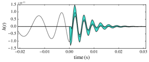
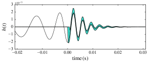
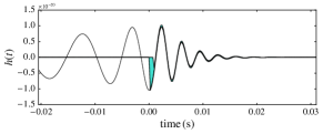
Figure 4: Left column: reconstructed post-merger waveform for the generic (GE) case (no relations among parameters are assumed) and corresponding $90\%$ confidence region (shaded area) for the GW150914-like dataset SXS:BBH:0305 with post-merger SNR = 10 (top panel), 20, 50 and 100 (bottom panel). Right column: the same, but for the constrained (CO) case, that assumes that an estimate for the component masses and spins exists. In all cases, the post-merger waveform is reconstructed very accurately, with uncertainty decreasing as the post-merger SNR increases.

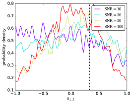
Figure 5: Measurability of the component masses $(m_{1},m_{2})$ and dimensionless spins $(s_{\bot,1},s_{\bot,2})$ for the GW150914-like dataset SXS:BBH:0305. The left panels show posterior distributions probabilities for the generic (GE) case (no relations among parameters are assumed) with post merger SNR = 10, 20, 50 and 100. The right panels refer to the constrained (CO) case, that assumes that an estimate for the component masses and spins exists. The vertical line in each panel indicates the correct value of the measured parameter.

Figure 6: Measurability of the fundamental QNM frequency $\omega_{1}$ (top), inverse damping time $\alpha_{1}$ (middle) and final black hole mass $M_{\rm BH}$ for the GW150914-like dataset SXS:BBH:0305. The left panels show posterior distributions probabilities for the GE case with post-merger SNR=10, 20, 50 and 100. The right panels refer to the CO case. The vertical line in each panel indicates the correct value of the measured parameter.

As a proof-of-principle, we investigated the accuracy of our template in a simplified, but realistic, scenario. In all cases we considered, and that are documented below in Sec.IV.2, we used our template for the inference of the physical parameters of a BBH from the post-merger part of the signal alone. We operate in the context of Bayesian inference; given the time series output of a detector $d(t)$, we model it as

$$d(t)=h(t;\theta)+n(t)\,,$$ (11)

where $n(t)$ is the detector noise time series and $h(t;\theta)$ is the GW signal depending on a set of physical parameters $\theta$. Given the time series $d(t)$ and a waveform model $h(t;\theta)$, our purpose is to compute the posterior probability distribution for $\theta$. To do so, we apply Bayes’ theorem:

$$p(\theta|d(t),I)=p(\theta|I)\frac{p(d(t)|\theta,I)}{p(d(t)|I)}\,,$$ (12)

where we introduced the prior probability density $p(\theta|I)$, the likelihood function $\mathcal{L}\equiv p(d(t)|\theta,I)$ and the evidence $p(d(t)|I)$. In all terms, we indicate with $I$ whatever background information is relevant to the inference in question. Since our template discontinuously passes from zero amplitude $A$ for $t<t_{0}$ to $A\neq 0$ for $t\geq t_{0}$, we find more convenient to perform the analysis in the time domain rather than in the frequency domain as it is done in most of the literature. Because of the discontinuity, the Fourier transform of our template would be contaminated by undesirable Gibbs phenomena which would make the inverse transform not consistent with the sharp time window that defines our template. This could be cured by the convolution in the frequency domain with the Fourier transform of a square window. However, we find simpler to perform the analysis directly in the time domain. For clarity, and also because this problem is typically reviewed in its frequency domain formulation, we will briefly go through the fundamentals of the statistical properties of the noise that, ultimately, are solely responsible for the specific functional form of the likelihood function $\mathcal{L}$. We assume, as customary, that the noise is described as a zero-mean wide-sense stationary Gaussian process. The probability distribution of any given noise realisation at some countable set of sampling times $t_{1},\ldots,t_{k}$ is thus given by

$$p(n_{1},\ldots,n_{k}|I) \propto e^{-\frac{1}{2}\sum_{i,j}C^{ij}n_{i}n_{j}}\,,$$ (13)

$$n_{i} \equiv n(t_{i})\,,$$ (14)

where ${C^{ij}}$ is the covariance matrix, defined by the stochastic process auto-covariance function $C(t_{i},t_{j})$:

$$C^{ij}\equiv C(t_{i},t_{j})\equiv<n(t_{j})n(t_{j})>\,.$$ (15)

Since the noise process is assumed to be wide-sense stationary, we can rewrite

$$C(t_{i}-t_{j},0)\equiv C(\tau)=<n(t)n(t+\tau)>\,.$$ (16)

The auto-covariance function $C(\tau)$ can be learnt from the data in a rather similar fashion to the Welch method for the estimation of the Power Spectral Density. However, for simplicity, we are going to assume that the noise process is white, thus $C(\tau)=\sigma^{2}\delta(\tau)$. The covariance matrix ${C^{ij}}$ is therefore diagonal and the probability distribution for the noise then simplifies to a product of one-dimensional Gaussian distributions

$$p(n_{1},\ldots,n_{k}|I)\propto e^{-\frac{1}{2}\sum_{i}\left(\frac{n_{i}}{\sigma}\right)^{2}}\,,$$ (17)

which is the functional form for the likelihood $\mathcal{L}$ that we will adopt throughout the rest of the paper.

IV.1 Simulation set up

Since the waveform of Eq. (1) depends on several parameters which allow for many possible degrees of freedom, we consider two set ups:

1. : The most generic (GE) case in which no relations among parameters are considered;

2. : Partially constrained (CO) case in which we assume that an estimate for the masses and spins of the progenitors exists and can be used to impose suitable priors when analyzing the post-merger part of signal with the template of Eq. (1);

For all cases, we fix the noise standard deviation $\sigma=5\times 10^{-22}$ and consider post-merger signal to noise ratios (SNR) of 10, 20, 50 and 100 by varying the distance $R$ to the source. Finally, we always consider the source to be optimally oriented and consider only one detector. We ignore the complications arising from projecting the signal onto the detector tensor since we are not interested in the inference of any extrinsic parameters like sky position or orientation. The set of parameters we consider in each case are:

1. : initial masses $(m_{1},m_{2})$, the (dimensionless) components of the spins orthogonal to the plane of the orbit $(s_{\bot,1},s_{\bot,2})$ (we adopt from now on the notation that $s_{\bot,1}$ and $s_{\bot,2}$ indicate the measured values of $\chi_{1}$ and $\chi_{2}$), the real, $\alpha_{1}$, and imaginary, $\omega_{1}$, parts of the fundamental mode complex frequency $\sigma_{1}=\alpha_{1}+{\rm i}\omega_{1}$ and the final BH mass $M_{\rm BH}$

2. : the parameters are the same as above, but with the distinction that the values of $(m_{1},m_{2})$ and $(s_{\bot,1},s_{\bot,2})$ have a restricted prior.

In addition to the aforementioned parameters, we always estimate the phase and time of merger $\phi_{0}$ and $t_{0}$ as well as the luminosity distance $R$.

For both GE and CO cases, we analyze all waveforms listed in Table 2. For simplicity, the total initial mass is always fixed to be $60M_{\odot}$ when simulating the detector time series. Finally, we consider a zero-noise realization. The data are analysed using a dedicated Nested Sampling algorithm cpn similar to Ref. Veitch et al. (2015).

IV.2 Results for GW150914-like dataset

We start by illustrating our findings through the GW150914-like system SXS:BBH:0305, that corresponds to $(q,\chi_{1},\chi_{2})\simeq(1.22,+0.33,-0.44)$. We show posterior distributions for the general case GE in Figs. 4 (waveform reconstruction) and in Figs. 5-6 for the posterior probability distributions of the various physical parameters. For all waveforms in Table 2, we compute posterior probability distributions for all the parameters listed in the previous Section and corresponding to the cases GE and CO. Figure 4 shows the $90\%$ confidence waveform recovered by our analysis as a function of the post-merger SNR going from 10 (top panel) to 100 (bottom panel). The left column is pertinent to the GE case while the right column to the CO case. In all cases one notices the shrinking of the $90\%$ credible region with increasing SNR. However, we also note two interesting facts: (i) the general behavior of the waveform is always well recovered, even in the lowest SNR case; (ii) there is not much difference between the GE and the CO case, indicating that, at least for systems like SXS:BBH:0305, the main factors determining the actual shape of the waveform are not much the initial properties of the coalescing system, but rather the properties of the final BH. This is further exemplified by looking at the details of the probability density functions (PDFs) given in Figs. 5 and 6. In the GE case, we see that the component masses $m_{1}$ and $m_{2}$ are largely unconstrained for SNR $<50$ and begin to be well measured ($O(30\%)$ and $O(20\%)$) for SNR = 50 and 100, respectively. At the same time, the spin magnitudes $s_{\bot,1}$ and $s_{\bot,2}$ are never constrained. We note a similar behavior for the ringdown part of the waveform. The QNM fundamental frequency $\omega_{1}$ can be constrained only when the post-merger SNR is $\geq 50$ while the (inverse) damping time $\alpha_{1}$ is always measured, improving to $O(25\%)$ and $O(15\%)$ for SNR = 50 and 100, respectively. Finally, we find that also the final black hole mass $M_{\mathrm{BH}}$ is measurable only for post-merger SNR $\geq 50$. In the CO case, the situation is remarkably similar. Apart from the obvious fact that the component masses are determined by their prior, no measurement of the component spins is possible, at least for the SNRs considered in this work. A main difference with the GE case is the accuracy with which the complex ringdown frequency can be determined. Remarkably, the posterior for $\omega_{1}$ does not seem to be affected the SNR considered which suggests that its posterior is mainly determined by correlations in the $m_{1},m_{2},\omega_{1}$ sub-parameter space; $\alpha_{1}$ instead is determined with $30\%,17\%,10\%$, and $8\%$ accuracy for SNR = $10,20,50,100$. Finally and not surprisingly also $M_{\mathrm{BH}}$ is always well determined, independently of the post-merger SNR.

Figure 7: Top panel: $90\%$ credible waveform for SXS:BBH:0185. Middle and bottom panels: posterior distributions probabilities for the general unconstrainded case for the fundamental QNM complex frequency for ${\rm SNR}=50$. The waveform reconstructed is well consistent with the underlying injected NR waveform, though the QNMs frequency show significan bias (the vertical line indicates the exact value).

IV.3 Results for the complete dataset

We then use the template to extract the parameters from all waveform listed in Table 2 and we report only on the (most demanding) GE case, i.e. no priors for the components masses and spins are assumed. The measured (complex) frequency of the fundamental QNM of the final BH as well as its mass $M_{\rm BH}$ are listed in the last columns of Table 2, either with post merger ${\rm SNR=10}$ and ${\rm SNR=50}$. Comparing the measured frequency with the exact value (third column in the table) one sees, on average, a good consistency between the measured and expect values. There are however a few exception, where the measured frequency looks biassed. Interestingly, we found that this effects persists also for ${\rm SNR>20}$, indicating that the template does show some systematics. For example, this is the case for $(9.99,0,0)$ and $(5,-0.90,0)$. The former case is illustrated in Fig. 7. The top panel shows the reconstructed $90\%$ waveform compared to the injected one for ${\rm SNR}=50$. This waveform is consistent with the expectations, suggesting that the functional ansatz we adopted are indeed appropriate to represent the true BBH waveform. However, the middle and lower panel in Fig. 7 show how biased is the complex frequency of the fundamental QNM. We speculate it to be due to the fact that this particular dataset stands outside the domain of calibration of the template (we recall that the largest mass-ratio we include is $q=8$) and that the extrapolation there is then not very accurate. To test whether this hypothesis is correct one will need to incorporate in the template (i) NR datasets with larger mass ratios (e.g., see e.g. Ref. Khan et al. (2016), that computed NR data with $q=18$) and (ii) large-mass ratio data Harms et al. (2014), though, as mentioned above, this will require, to be accurate, a new ansatz for the fitting template. For the case $(5,-0.90,0)$, the bias is probably due to the fact that the template is unable to account for the mixing between prograde and retrograde modes, an effect that, as mentioned already above, is evident when inspecting the phase difference in Fig. 3. Improving the post-merger waveform model with the primary goal of not having this biases will be our primary aim for future work.

IV.4 Testing the second law of BH dynamics

The specific nature of our template allows us to determine the initial masses and spins as well as the final mass and spin (the latter via the fundamental QNM) in an essentially independent fashion. In 1971 and 1972, Hawking proposed and proved the so-called “area theorem” or “second law of black hole dynamics” Hawking (1972); Bardeen et al. (1973):

when black holes collide the sum of the surface areas of all black holes involved can never decrease Misner et al. (1973).

By comparing the component masses and spins with the final mass and spin inferred from our analysis, we can compare the sum of the initial Kerr areas of the black hole binary with the Kerr area of the final black hole, without assuming a full coherent inspiral-merger-ringdown waveform that, being built on General Relativity, naturally satisfies the area theorem. We compare the posterior distributions on the Kerr areas as follows. Define $A_{1}+A_{2}=X$ the sum of the initial areas and $A_{f}$ is the area of the final black hole. For any Kerr black hole:

$$r_{s} =\frac{GM}{c^{2}},$$ (18)

$$A =4\pi(r_{+}^{2}+(ar_{s})^{2}),$$ (19)

$$r_{+} =r_{s}\left[1+\sqrt{1-a^{2}},\right]$$ (20)

with $M$ the black hole mass and $a$ the dimensionless spin parameter. Our purpose is to calculate $p(A_{f}\geq A_{1}+A_{2})$. If $f(A_{f})$ is the probability density function for $A_{f}$ and $g(A_{1}+A_{2})$ is the one for the sum of the initial areas, we define a new variable $z=A_{f}-(A_{1}+A_{2})$ and calculate

$$p(z)=\int dA_{f}f(A_{f})g(A_{f}-z),$$ (21)

from which it is possible to compute the probability that the final area is greater than the sum of the initial. For the GW150914-like dataset SXS:BBH:0305, we find probabilities $(0.74,0.74,0.78,0.85)$, respectively for ${\rm SNR}=(10,20,50,100)$, that the final area is larger than the initial one. This preliminary result illustrates the feasibility of this measurement. We will report an an extensive investigation of this aspect in a future publication.

V Concluding remarks

We proposed a post-merger, time-domain, waveform template of the form

$$h(\tau)=e^{-\sigma_{1}\tau-{\rm i}\phi_{0}}\bar{h}(\tau;\nu,{\hat{a}}_{0}),$$ (22)

where $\tau=(t-t_{0})/M_{\rm BH}$, ${\hat{a}}_{0}={\tilde{a}}_{1}+{\tilde{a}}_{2}$ and $\nu=m_{1}m_{2}/(m_{1}+m_{2})^{2}$. The complex fundamental QNM frequency $\sigma_{1}\equiv\alpha_{1}+{\rm i}\omega_{1}$ is itself a free parameter. We have also shown that this waveform is accurate and does provide a useful template to analyze the post-merger signal of systems like GW150914 that depends on the physical parameters of the system. In particular, modelling the post-merger part of the coalescence, the analysis presented in Ref. Abbott et al. (2016b), could be improved by either fixing the initial time $t_{0}$ much closer to the merger time $t_{\rm M}$, thus recovering more SNR, or marginalizing over the initial time $t_{0}$ so to avoid arbitrary choices for the beginning of the ringdown. Our template also provides a way of improving the inspiral-merger-ringdown consistency test Abbott et al. (2016b). The current test relies on the comparison of the posteriors reconstructed assuming the same waveform model in different frequency regimes. Our template provides an independent way of extracting physical information about the BBH system from the post-merger phase only. In principle, our template also gives a means to extract the full information about the original binary from a detailed analysis of the post-merger/ringdown signal. The feasibility and SNR requirements of this are currently being explored. Finally, the functional representation of the post-merger part given by Eq. (22) is easily generalized to allow for more freedom in the waveform. Some of the physical parameters entering in the vector $Y$ could be treated as free parameters and thus inferred from the data rather than being extracted from the NR simulations. For instance, in case of $\alpha_{1}$ and $\alpha_{2}$, i.e. the inverse damping time of the fundamental QNM and of the first overtone, one could relax the constraint $\alpha_{21}=\alpha_{2}-\alpha_{1}$ and keeping $\alpha_{1}$ as a free parameter in $\bar{h}$. Rather than Eq. (22), one would use a post-merger template of the form

$$h(\tau)=e^{-(\alpha_{1}+{\rm i}\omega_{1})\tau-{\rm i}\phi_{0}}\bar{h}(\tau;\nu,{\hat{a}}_{0},\alpha_{1},\alpha_{2}),$$ (23)

where $(\alpha_{1},\alpha_{2},\omega_{1})$ are all considered free parameters to be inferred from the experimental data. Measuring $\alpha_{2}$, one could setup a (partial) test of the general-relativistic no-hair theorem Dreyer et al. (2004); Berti et al. (2006, 2007); Gossan et al. (2012); Meidam et al. (2014) by estimating the consistency between $(\omega_{1},\alpha_{1})$ and $\alpha_{2}$.