Top quark mass effects in Higgs boson pair production up to NNLO

Abstract:

We consider the production of pairs of Standard Model Higgs bosons via gluon fusion. Until recently the full dependence on the top quark mass $M_{t}$ was not known at next-to-leading order. For this reason we apply an approximation based on the expansion for large top quark masses up to $\mathcal{O}(1/M_{t}^{12})$. At next-to-next-to-leading order we avoid the calculation of real corrections via the soft-virtual approximation and obtain top quark mass corrections up to $\mathcal{O}(1/M_{t}^{4})$. We use our results to estimate the residual uncertainty of the total cross section due to a finite top quark mass to be $\mathcal{O}(10\%)$ at next-to-leading order and $\mathcal{O}(5\%)$ at next-to-next-to-leading order.

1 Introduction

Higgs boson pair production is the process at the LHC that may in the future allow for an independent measurement of the cubic Higgs coupling. With this extraction a test whether the form of the Higgs potential is consistent with the Standard Model (where the cubic coupling is fixed by the Higgs bosons’ mass $m_{H}$ and its vacuum expectation value) and thereby of the mechanism of spontaneous symmetry breaking would be faciliated.

The dominant production mode is, as for single Higgs boson production although with a relative suppression of $\mathcal{O}(10^{-3})$, gluon fusion. The leading order (LO) calculation was performed retaining the exact dependence on the top quark mass $M_{t}$ in Refs. [1, 2]. Next-to-leading order (NLO) and next-to-next-to-leading order (NNLO) corrections were first calculated in the effective theory where the top quark is integrated out. See Ref. [3] for the NLO and Refs. [4, 5] for the NNLO case. Note that the matching coefficient for Higgs boson pairs differs starting from three loops from the one for a single Higgs boson, see Ref. [6].

Top quark mass corrections at NLO using a systematic expansion in $1/M_{t}$ were first studied in Refs. [7, 8, 9] and in Ref. [10] this calculation was extended to NNLO. In Ref. [11] the exact dependence on $M_{t}$ was taken into account for the real NLO corrections. Meanwhile the full NLO result became available taking into account the exact dependence on $M_{t}$ also for the virtual corrections, see Ref. [12]. For low center-of-mass energies, say between $\sqrt{s}=2m_{H}$ and $\sqrt{s}=2M_{t}$ the numerical uncertainties of Ref. [12] are still quite big whereas the expansions performed in Refs. [7, 10] show a good convergence behaviour. On the other hand, for higher center-of-mass energies the results of Refs. [7, 10] can only be used to obtain the order of magnitude of the $M_{t}$ effects which were estimated to be $\pm 10$ at NLO which is somewhat smaller than the results reported in Ref. [12].

In this contribution we describe the NNLO calculation of Ref. [10]. We start with full-theory diagrams where the top quark has not been integrated out. We apply the optical theorem on $gg\to gg$ forward scattering diagrams to extract the imaginary parts corresponding to real corrections $gg\to HH+X$ with additional partons $X$ in the final state. Virtual corrections are calculated directly from $gg\to HH$ amplitudes by squaring and integration over the $HH$ phase space. As a cross check we compute also virtual corrections via the optical theorem. In Fig. 1 we show some sample diagrams within the optical theorem approach. Note, at NLO (NNLO) we have to consider $gg\to HH$ amplitudes with two (three) or $gg\to gg$ forward scattering amplitudes with four (five) loops.

Figure 1: Sample forward scattering diagrams for the $gg$ channel. Curly lines represent gluons, dashed lines Higgs bosons and solid lines top quarks. The wavy line denotes a cut. The first row shows real corrections at NLO, the second row virtual corrections at NNLO.

2 Calculation

2.1 Differential factorization

The partonic cross section for the production of a pair of Higgs bosons via gluon fusion has the perturbative expansion

$$\begin{aligned} \sigma_{ij\to HH+X}(s,\rho)&=\delta_{ig}\delta_{jg}\sigma_{gg}^{(0)}(s,\rho)+\frac{\alpha_{s}}{\pi}\sigma_{ij}^{(1)}(s,\rho)+\left(\frac{\alpha_{s}}{\pi}\right)^{2}\sigma_{ij}^{(2)}(s,\rho)+\ldots\\[6.0pt] &=\sigma^{\text{LO}}+\delta\sigma^{\text{NLO}}+\delta\sigma^{\text{NNLO}}+\ldots,\end{aligned}$$ (1)

where we consider in the following only the dominant $gg$ channel with $i=j=g$. The variable $\rho=m_{H}^{2}/M_{t}^{2}$ describes the dependence on the Higgs boson and top quark masses. For convenience we absorb powers of $\alpha_{s}$ in the second line of Eq. (1).

The factorization of the LO result can be performed at the level of the differential cross section, see Ref. [3]:

$$\sigma^{(i)}=\int_{4m_{H}^{2}}^{s}\operatorname{d}\!Q^{2}\frac{\Big{(}\frac{\operatorname{d}\!\sigma_{\text{exact}}^{(0)}}{\operatorname{d}\!Q^{2}}\Big{)}}{\Big{(}\frac{\operatorname{d}\!\sigma_{\text{exp}}^{(0)}}{\operatorname{d}\!Q^{2}}\Big{)}}\frac{\operatorname{d}\!\sigma_{\text{exp}}^{(i)}}{\operatorname{d}\!Q^{2}}\quad\text{with}\quad\frac{\operatorname{d}\!\sigma_{\text{exp}}^{(i)}}{\operatorname{d}\!Q^{2}}=\sum_{n=0}^{N}c_{n}^{(i)}\rho^{n},$$ (2)

where “exact” refers to the LO result with full dependence on $\rho$, “exp” to the expansion for small $\rho$ and $Q^{2}$ is the invariant mass of the Higgs boson pair. The functional dependence of $\operatorname{d}\!\sigma_{\text{exact}}^{(0)}/\operatorname{d}\!Q^{2}$ and $\operatorname{d}\!\sigma_{\text{exp}}^{(i)}/\operatorname{d}\!Q^{2}$ in Eq. (2) are assumed to be similar in the region where $Q^{2}\gtrsim 4M_{t}^{2}$ which is expected to lead to a well behaved integrand. Note that we require the series expansions in numerator and denominator to be truncated at the same order $N$.

Within the framework described in Ref. [7] we computed the real NLO corrections via the forward scattering amplitude $gg\to gg$ using the optical theorem. For this reason we have no immediate access to the $Q^{2}$ dependence for these contributions. In contrast, the virtual corrections have a trivial $Q^{2}$ dependence $\delta(s-Q^{2})$ and are available to us from the direct calculation of the $gg\to HH$ amplitude.

2.2 Soft-virtual approximation

The obstacle we pointed out can be circumvented by applying the soft-virtual approximation, cf. Ref. [13]. We split a cross section $\sigma$ up according to

$$\sigma=\text{finite}=\sigma^{\text{virt}+\text{ren}}+\sigma^{\text{real}+\text{split}}=\underbrace{\Sigma_{\text{div}}\;+\;\Sigma_{\text{fin}}\quad+\quad\Sigma_{\text{soft}}}_{=\Sigma_{\text{SV}}}\;+\;\underbrace{\Sigma_{\text{hard}}}_{=\Sigma_{\text{H}}}.$$ (3)

The finite cross section is composed of virtual correction and renormalization pieces $\sigma^{\text{virt}+\text{ren}}$ and real correction and infrared counterterm pieces $\sigma^{\text{real}+\text{split}}$. These pieces in turn can be split up further: divergent terms $\Sigma_{\text{div}}$ and finite terms $\Sigma_{\text{fin}}$ for the former, divergent “soft” terms $\Sigma_{\text{soft}}$ and finite “hard” terms $\Sigma_{\text{hard}}=\Sigma_{\text{H}}$ for the latter. The sum of the first three terms on the right-hand side of Eq. (3) is finite and comprises the soft-virtual approximation. Note that this splitting holds also for differential cross sections $\operatorname{d}\!\sigma/\operatorname{d}\!Q^{2}$.

$\Sigma_{\text{div}}$ is universal for color-less final states and can be found in Refs. [6, 13]. We obtain $\Sigma_{\text{fin}}$ by computing $\sigma^{\text{virt}+\text{ren}}$ as expansion in $\rho$ and solving $\sigma^{\text{virt}+\text{ren}}=\Sigma_{\text{div}}+\Sigma_{\text{fin}}$. $\Sigma_{\text{div}}$ and $\Sigma_{\text{soft}}$ are proportional to $\sigma^{\text{LO}}$ and therefore automatically include effects due to finite $M_{t}$. We write the differential and total cross sections as

$$Q^{2}\frac{\operatorname{d}\!\sigma}{\operatorname{d}\!Q^{2}} =\sigma^{\text{LO}}zG(z)\quad\text{with}\quad G\!\left(z\right)=G_{\text{SV}}\!\left(z\right)+G_{\text{H}}\!\left(z\right),\quad z=\frac{Q^{2}}{s},$$ (4)

$$\sigma =\int_{1-\delta}^{1}\operatorname{d}\!z\sigma^{\text{LO}}(zs)G(z)\quad\text{with}\quad\delta=1-\frac{4m_{H}^{2}}{s},$$ (5)

where omitting $G_{\text{H}}(z)$ means using the soft-virtual approximation. $G_{\text{SV}}(z)$ is constructed from $\sigma_{\text{fin}}^{(i)}$ and $\sigma^{\text{LO}}$ only and can be found in Refs. [10, 13].

2.3 Asymptotic expansion

Let us briefly describe the computation of the diagrams as an expansion in $\rho$. The integrands of Feynman integrals are expanded according to a hierarchy of scales $M_{t}^{2}\gg m_{H}^{2},s$ for all possible scalings of loop momenta, so-called “regions”, and summed afterwards. The outcome of this procedure is a reduction of scales and loops which have to be considered at the same time (diagrams factorize). In case of an expansion for a hard mass all relevant regions correspond to subgraphs which must contain all heavy lines. For illustration we sketch the expansion regions for a virtual NLO diagram in the forward scattering approach in Fig. 2. Two regions emerge: one with a “soft” two-loop four-point graph multiplied with two “hard” one-loop tadpoles and one with a soft one-loop four-point graph multiplied with hard one- and two-loop tadpoles.

$M_{t}^{2},m_{H}^{2},s$ $\longrightarrow$ $M_{t}^{2}$ $\times$ $m_{H}^{2},s$ $\times$ $M_{t}^{2}$    +    $M_{t}^{2}$ $\times$ $m_{H}^{2},s$ $\times$ $M_{t}^{2}$

Figure 2: Asymptotic expansion in $M_{t}^{2}\gg m_{H}^{2},s$ applied to a virtual NLO forward scattering diagram, resulting in two different regions. Curly lines are gluons, dashed lines are the (cut) Higgs bosons and thick blue lines represent the top quarks. Each (sub)diagram is labeled with the scales it involves.

2.4 Software setup

Our software setup is highly automated, but we omit a detailed survey here and refer instead to Ref. [10] where also intermediate results are given and the calculation of the master integrals is discussed. We generate diagrams with QGRAF [14] where in the case of $gg\to gg$ postprocessing [9, 15] is mandatory. For topology identification and other steps of the calculation we use the package TopoID [9, 15]. Asymptotic expansion and mapping of diagrams to topologies is performed with q2e and exp [16, 17]. The reduction to scalar integrals uses FORM [18]. Soft four-point subdiagrams are reduced to master integrals with FIRE [19, 20] and the in-house code rows [15]. Hard subdiagrams are always massive tadpoles and can be treated with MATAD [21].

3 Results

We summarize the main features of our findings in bullet points. For details, such as the particular values of input parameters, cf. Ref. [10]. Throughout the presented analysis we set the renormalization scale to $\mu=2m_{H}$ and use the MSTW2008 PDFs [22].

• In a split-up (not shown) of the NLO correction to the total partonic cross section into soft-virtual and hard contributions, we observe different patterns when including higher $\rho$ corrections: soft-virtual corrections increase, whereas hard ones descrease with $\sqrt{s}$. Soft-virtual corrections dominate over the full range of $\sqrt{s}$, above $400\,\text{GeV}$ hard ones become flat.

• In Fig. 3 we show results for hadronic quantities. We introduced a technical upper cut-off for the partonic center-of-mass energy $\sqrt{s_{\text{cut}}}$ which is a good approximation to the invariant mass of the produced Higgs boson pair:

  $$\sigma_{H}(s_{H},s_{\text{cut}})=\int_{4m_{H}^{2}/s_{H}}^{1}\operatorname{d}\!\tau\left(\frac{\operatorname{d}\mathcal{L}_{gg}}{\operatorname{d}\!\tau}\right)\!(\tau)\sigma(\tau s_{H})\theta(s_{\text{cut}}-\tau S_{H}),$$ (6)

  where $\sqrt{s_{H}}=14\,\text{TeV}$ is the hadronic center-of-mass energy for the LHC and $\mathcal{L}_{gg}$ is the luminosity function for two gluons in the inital state.

  From the spread of $\rho$ orders for the total hadronic cross section $\sigma_{H}^{\text{NLO}}$ on the right-hand side, when $\sqrt{s_{\text{cut}}}\to\infty$, we infer the uncertainty due to top quark mass corrections to be about $\pm 10\%$.

  

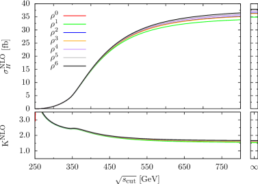
  Figure 3: NLO hadronic cross section $\sigma_{H}^{\text{NLO}}$ in the upper panel and $K$ factor $K^{\text{NLO}}$ in the lower panel as functions of $\sqrt{s_{\text{cut}}}$, a technical upper cut on $\sqrt{s}$ and proxy to the invariant mass of the Higgs boson pair. We use “$\infty$” to symbolize the results for the total inclusive cross section and $K$ factor on the right-hand side. Here and in the following the color coding indicates the inclusion of higher orders in the $\rho$ expansion. Figure taken from Ref. [10].

• In the soft-virtual approximation $G_{\text{SV}}(z)$ from Eq. (3) can be replaced by $f(z)G_{\text{SV}}(z)$ with any $f(z)$ fulfilling $f(1)=1$ since the splitting into hard and soft-virtual components is not unique. At NLO we observe that using $f(z)=z$ and neglecting hard contributions is accurate within $2\%$. Also, replacing $\log(\mu^{2}/s)$ by $\log(\mu^{2}/Q^{2})$ leads to better results which can be justified in the soft limit where $s\approx Q^{2}$. We adopt these prescriptions to proceed at NNLO.

• In Fig. 4 we recognize for the LO, NLO and NNLO corrections $\delta\sigma$ the same pattern in the $\rho$ expansion (negative shifts for $\rho^{1}$ and positive ones for $\rho^{2}$) and that the peak positions move to lower values for $\sqrt{s}$ for higher perturbative orders.

  

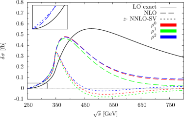
  Figure 4: LO, NLO and NNLO contributions $\delta\sigma$ to the partonic cross section. At LO the exact result is shown as solid black line, at NLO and NNLO we give only the first three expansion orders in $\rho$ for consistency and we use $f(z)=z$ at NNLO (see the main text). The inset magnifies the region of small $\sqrt{s}$. Figure taken from Ref. [10].

• For the total hadronic cross section $\sigma_{H}$ up to NNLO in Fig. 5 we find good convergence up to $\sqrt{s_{\text{cut}}}\approx 400\,\text{GeV}$ and deduce in the same way as on NLO an uncertainty due to the top quark mass of about $\pm 5\%$ (note that NNLO corrections within the effective theory amount to about $20\%$ by themselves).

  

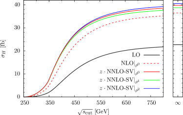
  Figure 5: LO, NLO and NNLO hadronic cross sections $\sigma_{H}$. At LO the exact is shown, at NLO we give only the leading expansion term and at NNLO the first three terms in $\rho$. On the right-hand side the total inclusive results are given. Figure taken from Ref. [10].

• In the behavior of the $K$ factor up to NNLO in Fig. 6 we see that the characteristic form around the $2M_{t}$ threshold is not washed out. The strong raise close to the $2m_{H}$ threshold is explained by the steepness of the NNLO correction, see the inset. The hadronic NNLO $K$ factor is in the range $1.7$ to $1.8$.

  

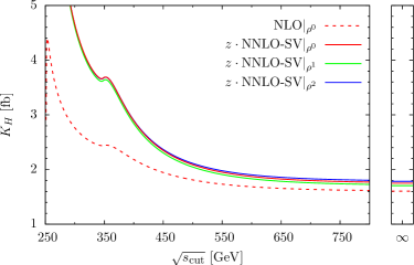
  Figure 6: LO, NLO and NNLO hadronic $K$ factors $K_{H}$. The notation is as in Fig. 5. Figure taken from Ref. [10].

4 Conclusion

We computed corrections due to a finite top quark mass using an asymptotic expansion in the limit $M_{t}^{2}\gg m_{H}^{2},s$. At NLO our method yields results up to $\mathcal{O}(1/M_{t}^{12})$, at NNLO up to $\mathcal{O}(1/M_{t}^{4})$ using the soft-virtual approximation. We estimate the residual error on the total cross section due to finite $M_{t}$ to be $\mathcal{O}(10\%)$ at NLO and $\mathcal{O}(5\%)$ at NNLO.

The recently completed full NLO contribution to the total cross section, see Ref. [12] and the presentations [23, 24], is decreased by $14\%$ compared to the $M_{t}\to\infty$ limit. For $Q^{2}\leq 400\,\text{GeV}$ effects of $\mathcal{O}(10\%)$ are reported for the differential cross section and even larger ones above $400\,\text{GeV}$.

The NNLO contributions yield a $\mathcal{O}(20\%)$ correction in the $M_{t}\to\infty$ limit which could be modified substantially by the $M_{t}$ dependence, but a full NNLO calculation is out of scope of present techniques. Therefore it seems disirable to refine our approximation procedure to better reproduce the findings of Ref. [12] and to revisit the NNLO case.

References

- [1] E. W. N. Glover and J. J. van der Bij, Nucl. Phys. B 309, 282 (1988). doi:10.1016/0550-3213(88)90083-1
- [2] T. Plehn, M. Spira and P. M. Zerwas, Nucl. Phys. B 479, 46 (1996) Erratum: [Nucl. Phys. B 531, 655 (1998)] doi:10.1016/0550-3213(96)00418-X [hep-ph/9603205].
- [3] S. Dawson, S. Dittmaier and M. Spira, Phys. Rev. D 58, 115012 (1998) doi:10.1103/PhysRevD.58.115012 [hep-ph/9805244].
- [4] D. de Florian and J. Mazzitelli, Phys. Lett. B 724, 306 (2013) doi:10.1016/j.physletb.2013.06.046 [arXiv:1305.5206 [hep-ph]].
- [5] D. de Florian and J. Mazzitelli, Phys. Rev. Lett. 111, 201801 (2013) doi:10.1103/PhysRevLett.111.201801 [arXiv:1309.6594 [hep-ph]].
- [6] J. Grigo, K. Melnikov and M. Steinhauser, Nucl. Phys. B 888, 17 (2014) doi:10.1016/j.nuclphysb.2014.09.003 [arXiv:1408.2422 [hep-ph]].
- [7] J. Grigo, J. Hoff, K. Melnikov and M. Steinhauser, Nucl. Phys. B 875, 1 (2013) doi:10.1016/j.nuclphysb.2013.06.024 [arXiv:1305.7340 [hep-ph]].
- [8] J. Grigo, J. Hoff, K. Melnikov and M. Steinhauser, PoS RADCOR 2013, 006 (2013) [arXiv:1311.7425 [hep-ph]].
- [9] J. Grigo and J. Hoff, PoS LL 2014, 030 (2014) [arXiv:1407.1617 [hep-ph]].
- [10] J. Grigo, J. Hoff and M. Steinhauser, Nucl. Phys. B 900, 412 (2015) doi:10.1016/j.nuclphysb.2015.09.012 [arXiv:1508.00909 [hep-ph]].
- [11] F. Maltoni, E. Vryonidou and M. Zaro, JHEP 1411, 079 (2014) doi:10.1007/JHEP11(2014)079 [arXiv:1408.6542 [hep-ph]].
- [12] S. Borowka, N. Greiner, G. Heinrich, S. P. Jones, M. Kerner, J. Schlenk, U. Schubert and T. Zirke, arXiv:1604.06447 [hep-ph].
- [13] D. de Florian and J. Mazzitelli, JHEP 1212, 088 (2012) doi:10.1007/JHEP12(2012)08, 10.1007/JHEP12(2012)088 [arXiv:1209.0673 [hep-ph]].
- [14] P. Nogueira, J. Comput. Phys. 105, 279 (1993). doi:10.1006/jcph.1993.1074
- [15] J. Hoff, “Methods for multiloop calculations and Higgs boson production at the LHC”, Dissertation, KIT, 2015.
- [16] R. Harlander, T. Seidensticker and M. Steinhauser, Phys. Lett. B 426, 125 (1998) doi:10.1016/S0370-2693(98)00220-2 [hep-ph/9712228].
- [17] T. Seidensticker, hep-ph/9905298.
- [18] J. Kuipers, T. Ueda, J. A. M. Vermaseren and J. Vollinga, Comput. Phys. Commun. 184, 1453 (2013) doi:10.1016/j.cpc.2012.12.028 [arXiv:1203.6543 [cs.SC]].
- [19] A. V. Smirnov and V. A. Smirnov, Comput. Phys. Commun. 184, 2820 (2013) doi:10.1016/j.cpc.2013.06.016 [arXiv:1302.5885 [hep-ph]].
- [20] A. V. Smirnov, Comput. Phys. Commun. 189, 182 (2015) doi:10.1016/j.cpc.2014.11.024 [arXiv:1408.2372 [hep-ph]].
- [21] M. Steinhauser, Comput. Phys. Commun. 134, 335 (2001) doi:10.1016/S0010-4655(00)00204-6 [hep-ph/0009029].
- [22] A. D. Martin, W. J. Stirling, R. S. Thorne and G. Watt, Eur. Phys. J. C 63 (2009) 189 doi:10.1140/epjc/s10052-009-1072-5 [arXiv:0901.0002 [hep-ph]].
- [23] M. Kerner, PoS LL 2016, 023 (2016)
- [24] S. Jones, PoS LL 2016, 069 (2016)