The Implicit Convex Feasibility Problem and Its Application to Adaptive Image Denoising

Abstract

The implicit convex feasibility problem attempts to find a point in the intersection of a finite family of convex sets, some of which are not explicitly determined but may vary. We develop simultaneous and sequential projection methods capable of handling such problems and demonstrate their applicability to image denoising in a specific medical imaging situation. By allowing the variable sets to undergo scaling, shifting and rotation, this work generalizes previous results wherein the implicit convex feasibility problem was used for cooperative wireless sensor network positioning where sets are balls and their centers were implicit.

Keywords: Implicit convex feasibility $\cdot$ split feasibility $\cdot$ projection methods $\cdot$ variable sets $\cdot$ proximity function $\cdot$ image denoising

1 Introduction

In this paper we are concerned with the following “implicit convex feasibility problem” (ICFP). Given set-valued mappings $C_{s}:\mathbb{R}^{n}\rightarrow 2^{\mathbb{R}^{n}}$, $s=1,2,\ldots,S,$ with closed and convex value sets, the ICFP is,

$$\text{Find a point }x^{\ast}\in\cap_{s=1}^{S}C_{s}(x^{\ast}).$$ (1.1)

We call the sets $C_{s}(x)$ “variable sets” for obvious reasons and include “implicit” in this problem name because the sets defining it are not given explicitly ahead of time. The problem is inspired by the work of Gholami et al. [21] on solving the cooperative wireless sensor network positioning problem in $\mathbb{R}^{2}$ ($\mathbb{R}^{n}$). There, the sets $C_{s}(x)$ are circles (balls) with varying centers. A special instance of the ICFP is obtained by taking fixed sets $C_{s}(x)\equiv C_{s},$ for all $x\in\mathbb{R}^{n},$ and all $s=1,2,\ldots,S,$ yielding the well-known, see, e.g., [3], “convex feasibility problem” (CFP) which is,

$$\text{Find a point }x^{\ast}\in\cap_{s=1}^{S}C_{s}.$$ (1.2)

The CFP formalism is at the core of the modeling of many inverse problems in various areas of mathematics and the physical sciences. This problem has been widely explored and researched in the last decades, see, e.g., [10, Section 1.3], and many iterative methods where proposed, in particular projection methods, see, e.g., [11]. These are iterative algorithms that use projections onto sets, relying on the principle that when a family of sets is present, then projections onto the given individual sets are easier to perform than projections onto other sets (intersections, image sets under some transformation, etc.) that are derived from the given individual sets.

Gholami et al. in [21] introduced the implicit convex feasibility problem (ICFP) in $\mathbb{R}^{d}$ ($d=2$ or $d=3$) into their study of the wireless sensor network (WSN) positioning problem. In their reformulation the variable sets are circles or balls whose centers represent the sensors’ locations and their broadcasting range is represented as the radii. Some of these centers are known a priori while the rest are unknown and need to be determined. The WSN positioning problem is to find a point, in an appropriate product space, which represents the circles or balls centers. The precise relationship between the WSN problem and the ICFP can be found in [21, Section B]. For more details and other examples of geometric positioning problems, see [20, 22].

We focus on the ICFP in $\mathbb{R}^{n}$ and present projection methods for its solution. This expands and generalizes the special case treated in Gholami et al. [21]. Moreover, we demonstrate the applicability of our approach to the task of image denoising, where we impose constraints on the image intensity at every image pixel. Because the constraint sets depend on the unknown variables to be determined, the method is able to adapt to the image contents. This application demonstrates the usefulness of the ICFP approach to image processing.

The paper is structured as follows. In Section 2 we show how to calculate projections onto variable sets. In Section 3 we present two projection type algorithmic schemes for solving the ICFP, sequential and simultaneous, along with their convergence proofs. In Section 4 we present the ICFP application to image denoising together with numerical visualization of the performance of the methods. Finally, in Section 5 we discuss further research directions and propose a further generalization of the ICFP.

2 Projections onto variable convex sets

We begin by recalling the split convex feasibility problem (SCFP) and the constrained multiple-set split convex feasibility problem (CMSSCFP) that will be useful to our subsequent analysis.

Problem 2.1

Censor and Elfving [13]. Given nonempty, closed and convex sets $C\subseteq\mathbb{R}^{n},$ $Q\subseteq\mathbb{R}^{m}$ and a linear operator $T:\mathbb{R}^{n}\rightarrow\mathbb{R}^{m}$, the Split Convex Feasibility Problem (SCFP) is:

$$\text{Find a point }x^{\ast}\in C\text{ such that }T(x^{\ast})\in Q.$$ (2.1)

Another related more general problem is the following.

Problem 2.2

Masad and Reich [31]. Let $r,p\in\mathbb{N}$ and $\Omega_{s},$ $1\leq s\leq{S},$ and $Q_{r},$ $1\leq r\leq{R},$ be nonempty, closed and convex subsets of $\mathbb{R}^{n}\$and $\mathbb{R}^{m},$ respectively. Given linear operators $T_{r}:\mathbb{R}^{n}\rightarrow\mathbb{R}^{m},$ $1\leq r\leq{R}$ and another nonempty, closed and convex $\Gamma\subseteq\mathbb{R}^{n}$, the Constrained Multiple-Set Split Convex Feasibility Problem (CMSSCFP) is:

$$\text{Find a point }x^{\ast}\in\Gamma\text{ such that}$$

$$x^{\ast}\in\cap_{s=1}^{S}\Omega_{s}\text{ and }T_{r}(x^{\ast})\in Q_{r}\text{ for each }r=1,2,\ldots,{R}.$$ (2.2)

If $T_{r}\equiv T$ for all $r=1,2,\ldots,{R}$, then we obtain a multiple-set split convex feasibility problem (MSSCFP) [14].

A prototype for the above SCFP and MSSCFP is the Split Inverse Problem (SIP) presented in [8, 15] and given next.

Problem 2.3

Given two vector spaces $X$ and $Y$ and a linear operator $A:X\rightarrow Y$, we look at two inverse problems. One, denoted by IP${}_{1},$ is formulated in $X$ and the second, denoted by IP₂, is formulated in $Y$. The Split Inverse Problem (SIP) is:

$$\text{Find a point }x^{\ast}\in X\text{ that solves IP}_{1}\text{such that }y^{\ast}=Ax^{\ast}\text{solves IP}_{2}.$$ (2.3)

In [8, 15] different choices for IP₁ and IP₂ are proposed, such as variational inequalities and minimization problems. The latter enable, for example, to obtain a least-intensity feasible solution in intensity-modulated radiation therapy (IMRT) treatment planning as in [39]. In [23] we further explore and extend this modeling technique to include non-linear mappings between the two spaces $X$ and $Y$.

Let $C\subseteq\mathbb{R}^{n}$ be a nonempty, closed and convex set. For each point $x\in\mathbb{R}^{n}$, there exists a unique nearest point in $C$, denoted by $P_{C}(x)$, i.e.,

$$\left\|x-P_{C}\left(x\right)\right\|\leq\left\|x-y\right\|,\text{ for all }y\in C.$$ (2.4)

The mapping $P_{C}:\mathbb{R}^{n}\rightarrow C$ is the metric projection of $\mathbb{R}^{n}$ onto $C$. It is well-known that $P_{C}$ is a nonexpansive mapping of $\mathbb{R}^{n}$ onto $C$, i.e.,

$$\left\|P_{C}\left(x\right)-P_{C}\left(y\right)\right\|\leq\left\|x-y\right\|,\ \text{for all }x,y\in\mathbb{R}^{n}.$$ (2.5)

The metric projection $P_{C}$ is characterized by the following two properties:

$$P_{C}(x)\in C$$ (2.6)

and

$$\left\langle x-P_{C}\left(x\right),y-P_{C}\left(x\right)\right\rangle\leq 0,\text{ for all }x\in\mathbb{R}^{n},\text{ }y\in C.$$ (2.7)

If $C$ is a hyperplane, then (2.7) becomes an equality, [24]. We are dealing with variable convex sets that can be described by set-valued mappings.

Definition 2.4

For a set-valued mapping $C:\mathbb{R}^{n}\rightarrow 2^{\mathbb{R}^{n}},$ we call the sets $C(x)\subseteq\mathbb{R}^{n},$ defined below, “variable sets”. Let $\Omega\subseteq\mathbb{R}^{n}$ be a given set, called in the sequel a “core set”.

(i) Given an operator $\mu:\mathbb{R}^{n}\rightarrow\mathbb{R}^{n}$, the variable sets $C(x):=\Omega+\mu(x)=\left\{y+\mu(x)\mid y\in\Omega\right\},$ for $x\in\mathbb{R}^{n}$, are obtained from shifting $\Omega$ by the vectors $\mu(x)$.

(ii) Given an $x\in\mathbb{R}^{n}$ let $U_{\left[x\right]}:\mathbb{R}^{n}\rightarrow\mathbb{R}^{n}$ be a linear bounded operator. The variable sets $C(x):=U_{\left[x\right]}(\Omega)=\left\{U_{\left[x\right]}y\mid y\in\Omega\right\}$ are the $U_{\left[x\right]}$ images of $\Omega$.

(iii) Given a function $f:\mathbb{R}^{n}\rightarrow\mathbb{R}_{+}$, the variable sets $C(x):=f(x)\Omega=\left\{f(x)y\mid y\in\Omega\right\},$ for $x\in\mathbb{R}^{n}$, are obtained from scaling $\Omega$ uniformly by $f(x)$. This can be re-written as in (ii) with $U_{\left[x\right]}=f(x)I$, where $I$ is the identity matrix.

Next we present a lemma that shows how to calculate the metric projection onto such variable sets via projections onto the core set $\Omega$ when the operator $\mu$ is linear and denoted by the fixed matrix $A$ and $U_{\left[x\right]}$ is a constant unitary matrix denoted by $U$ (that is $U^{T}U=UU^{T}=I$, where $U^{T}:\mathbb{R}^{n}\rightarrow\mathbb{R}^{n}$ is the adjoint of $U$). Our proofs are based on Cegielski [10, Subsection 1.2.3].

Lemma 2.5

Let $\Omega\subseteq\mathbb{R}^{n}$ be a nonempty, closed and convex core set. Given a matrix $A$, a positive diagonal matrix $D=\alpha I,$ $\alpha>0,$ and a fixed unitary matrix $U$, the following holds for any $z,x\in\mathbb{R}^{n}$

$$P_{DU\left(\Omega\right)+Ax}\left(z\right)=DUP_{\Omega}\left(D^{-1}U^{T}\left(z-Ax\right)\right)+Ax.$$ (2.8)

Since $D$ is a positive diagonal matrix, this can be re-written as

$$P_{C(x)}\left(z\right)=\alpha UP_{\Omega}\left(\frac{1}{\alpha}U^{T}\left(z-Ax\right)\right)+Ax$$ (2.9)

where $C(x)=\alpha U\left(\Omega\right)+Ax.$

Proof. Let $z\in\mathbb{R}^{n}$ and denote

$$y:=\alpha UP_{\Omega}\left(\frac{1}{\alpha}U^{T}\left(z-Ax\right)\right)+Ax.$$ (2.10)

We show that

$$y=P_{C(x)}\left(z\right).$$ (2.11)

From (2.10) and the unitary matrix $U$ we deduce

$$\frac{1}{\alpha}U^{T}\left(y-Ax\right)=P_{\Omega}\left(\frac{1}{\alpha}U^{T}\left(z-Ax\right)\right).$$ (2.12)

By the characterization of the metric projection onto $\Omega$ (2.7) we have

$$\left\langle\frac{1}{\alpha}U^{T}\left(z-Ax\right)-\frac{1}{\alpha}U^{T}\left(y-Ax\right),w-\frac{1}{\alpha}U^{T}\left(y-Ax\right)\right\rangle\leq 0,\text{ for all }w\in\Omega.$$ (2.13)

Since $\alpha>0$ and $U$ is unitary, we get

$$\left\langle z-y,\alpha Uw+Ax-y\right\rangle\leq 0,\text{ for all }w\in\Omega.$$ (2.14)

Denoting $v:=\alpha Uw+Ax$, since $w\in\Omega$ we get $v\in\alpha U\left(\Omega\right)+Ax=C(x)$,

the

$$\left\langle z-y,v-y\right\rangle\leq 0,\text{ for all }v\in C(x),$$ (2.15)

and again by the characterization of the metric projection onto $C(x)$ (2.7) and by (2.10) $y=P_{C(x)}\left(z\right)$ which completes the proof.   

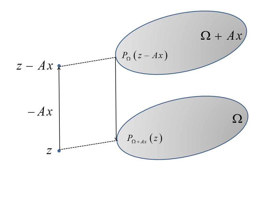
Figure 1: Illustration of Lemma 2.5 with $D,U=I$

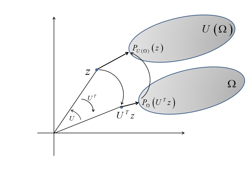
Figure 2: Illustration of Lemma 2.5 with $D=I$ and $A=0$

Two special cases of Lemma 2.5 are illustrated. In Figure 1 we use $D,U=I$ so that $P_{\Omega+Ax}\left(z\right)=P_{\Omega}\left(z-Ax\right)+Ax$, meaning that the set $\Omega$ is shifted by the point $Ax$ to $\Omega+Ax$. In Figure 2 we use $D=I$ and $A=0$ so that $P_{U\left(\Omega\right)}\left(z\right)=UP_{\Omega}\left(U^{T}z\right)$, meaning that the set $\Omega$ is rotated by the unitary matrix $U$ to $U\left(\Omega\right)$.

3 The algorithms

The following definitions will be used.

Definition 3.1

A sequence $\{\sigma_{k}\}_{k\in\mathbb{N}}$ of real positive numbers is called a steering sequence if it satisfies all the following conditions: (i) $\lim_{k\rightarrow\infty}\sigma_{k}=0;$ (ii) $\lim_{k\rightarrow\infty}\frac{\displaystyle\sigma_{k+1}}{\displaystyle\sigma_{k}}=1;$ and (iii) $\sum_{k=0}^{\infty}\sigma_{k}=+\infty.$ Let $\beta$ be a positive integer. If condition (ii) is replaced by

$$\lim_{k\rightarrow\infty}\frac{\sigma_{k\beta+j}}{\sigma_{k\beta}}=1,\ \text{for all }1\leq j\leq\beta-1,$$ (3.1)

and  (i) and (iii) remain unchanged then the sequence is called an $\beta$-steering sequence.

Definition 3.2

A sequence $\{i(k)\}_{k\in\mathbb{N}}$ of indices is called a cyclic control sequence over the index set $\{1,2,\ldots,S\}$ if

$$i(k)=k\operatorname{mod}S,\text{ \ for }k\geq 0.$$ (3.2)

Problem 3.3

The Implicit Convex Feasibility Problem. Given set-valued mappings $C_{s}:\mathbb{R}^{n}\rightarrow 2^{\mathbb{R}^{n}}$, $s=1,2,\ldots,{S,}$ with closed convex values $C_{s}(x)$, the Implicit Convex Feasibility Problem (ICFP) is

$$\text{Find a point }x^{\ast}\in\cap_{s=1}^{S}C_{s}(x^{\ast}).$$ (3.3)

One way of handling this problem is to reformulate it as the unconstrained minimization

$$\left\{\begin{array}[c]{ll}\mathrm{minimize}&G_{icfp}(x)\\ \mathrm{subject~{}to}&x\in\mathbb{R}^{n},\end{array}\right.$$ (3.4)

where

$$G_{icfp}(x):=\frac{1}{2}\sum_{s=1}^{S}\|x-P_{C_{s}(x)}(x)\|^{2}$$ (3.5)

in which $P_{C_{s}(x)}$ is the metric projection operator onto the sets $C_{s}(x)$.

Following the works of Censor et al. [12] and Gholami et al. [21] we present two algorithmic schemes, simultaneous and sequential, for solving the ICFP of Problem 3.3. For $s=1,2,\ldots,{S,}$ let $\Omega_{s}$ be nonempty, closed and convex core sets in $\mathbb{R}^{n}$, $A_{s}\in\mathbb{R}^{n\times n}$ are matrices, $U_{s}\in\mathbb{R}^{n\times n}$ are unitary matrices, and $\alpha_{s}>0$. Then the variable sets defined in Definition 2.4 take the form

$$C_{s}(x)=\alpha_{s}U_{s}\left(\Omega_{s}\right)+A_{s}x,$$ (3.6)

and we assume that the projection $P_{\Omega_{s}}$ are at hand or can be easily calculated.

Algorithm 3.4

The Simultaneous Algorithm

Preliminary calculations: For $s=1,2,\ldots,{S,}$ calculate the matrices

$$K_{s}:=\frac{1}{\alpha_{s}}U_{s}^{T}\left(I-A_{s}\right)$$ (3.7)

and use matrix $2$-norms to calculate the constant

$$L_{icfp}=\sum_{s=1}^{S}\left\|I-A_{s}\right\|_{2}^{2}.$$ (3.8)

Initialization: Select an arbitrary starting point $x^{0}\in\mathbb{R}^{n}$ and set $k=0$.

Iterative step: Given the current iterate $x^{k}$, calculate the next iterate by

$$x^{k+1}=x^{k}-\gamma_{k}\sum_{s=1}^{S}\alpha_{s}^{2}K_{s}^{T}\left(I-P_{\Omega_{s}}\right)\left(K_{s}x^{k}\right),$$ (3.9)

where $\gamma_{k}\in(0,2/L_{icfp})$ for all $k\geq 0.$

Stopping rule: If $x^{k+1}=x^{k}$ (or, alternatively, if $\|x^{k+1}-x^{k}\|$ is small enough) then stop. Otherwise, set $k\leftarrow(k+1)$ and go back to the beginning of the iterative step.

Algorithm 3.5

The Sequential Algorithm

Preliminary calculation: For $s=1,2,\ldots,{S,}$ calculate the matrices

$$K_{s}:=\frac{1}{\alpha_{s}}U_{s}^{T}\left(I-A_{s}\right).$$ (3.10)

Initialization: Select an arbitrary starting point $x^{0}\in\mathbb{R}^{n}$ and set $k=0$.

Iterative step: Given the current iterate $x^{k}$, calculate the next iterate by

$$x^{k+1}=x^{k}-\sigma_{k}\alpha_{i(k)}^{2}K_{i(k)}^{T}\left(I-P_{\Omega_{i(k)}}\right)\left(K_{i(k)}x^{k}\right),$$ (3.11)

where $\{\sigma_{k}\}_{k\in\mathbb{N}}$ and $\{i(k)\}_{k\in\mathbb{N}}$ are a $\beta$-steering and a cyclic control sequences, respectively.

Stopping rule: If $x^{k+1}=x^{k}$ (or, alternatively, if $\|x^{k+1}-x^{k}\|$ is small enough) then stop. Otherwise, set $k\leftarrow(k+1)$ and go back to the beginning of the iterative step.

3.1 Convergence

For the mappings $C_{s}(\cdot)$ of (3.6) we get, from Lemma 2.5, a simplified form of the proximity function $G_{icfp}$ in (3.5),

$$G_{icfp}(x) =\frac{1}{2}\sum_{s=1}^{S}\left\|x-\left(\alpha_{s}U_{s}P_{\Omega_{s}}\left(\frac{1}{\alpha_{s}}U_{s}^{T}\left(x-A_{s}x\right)\right)+A_{s}x\right)\right\|^{2}$$

$$=\frac{1}{2}\sum_{s=1}^{S}\left\|\alpha_{s}U_{s}\left(I-P_{\Omega_{s}}\right)\left(\frac{1}{\alpha_{s}}U_{s}^{T}\left(I-A_{s}\right)x\right)\right\|^{2}$$

$$=\frac{1}{2}\sum_{s=1}^{S}\alpha_{s}^{2}\left\|\left(I-P_{\Omega_{s}}\right)\left(\frac{1}{\alpha_{s}}U_{s}^{T}\left(I-A_{s}\right)x\right)\right\|^{2}$$

$$=\frac{1}{2}\sum_{s=1}^{S}\alpha_{s}^{2}\left\|\left(I-P_{\Omega_{s}}\right)\left(K_{s}x\right)\right\|^{2},$$ (3.12)

where $K_{s}$ is as in (3.7).

In order to prove convergence of Algorithm 3.4 we need to show that the function $G_{icfp}$ is convex, continuously differentiable and that its gradient is Lipschitz continuous (see [21, Proposition 4]). For the convergence of Algorithm 3.5 it is sufficient to show only convexity and continuous differentiability of $G_{icfp}$, see [12, Theorem 6]. In both cases our analysis relies on the classical theorems of Baillon and Haddad [2] and of Dolidze [18].

Proposition 3.6

The function $G_{icfp}$ of (3.12) is (1) convex, (2) continuously differentiable, and (3) its gradient is Lipschitz continuous.

Proof. Recall that the SCFP (2.1) can also be formulated as the minimization problem

$$\left\{\begin{array}[c]{ll}\mathrm{minimize}&G_{scfp}(x):=\frac{1}{2}\left\|Tx-P_{Q}\left(Tx\right)\right\|^{2}\\ \mathrm{subject~{}to}&x\in C,\end{array}\right.$$ (3.13)

see, e.g., [7], and, moreover, for the CMSSCFP (2.2) we have

$$\left\{\begin{array}[c]{ll}\mathrm{minimize}&G_{cmsscfp}(x):=\frac{1}{2}\sum_{s=1}^{S}\left\|x-P_{\Omega_{s}}\left(x\right)\right\|^{2}+\frac{1}{2}\sum_{r=1}^{R}\left\|T_{r}x-P_{Q_{r}}\left(T_{r}x\right)\right\|^{2}\\ \mathrm{subject~{}to}&x\in\Gamma,\end{array}\right.$$ (3.14)

see [31]. Since our proximity function $G_{icfp}$ (3.12) shares some common features with the above $G_{scfp}$ and $G_{cmsscfp}$ functions, we follow the lines of [31] and [21, Theorem 2] to prove the proposition.

(1) The convexity of $G_{icfp}$ (3.12) is obvious, see, for example [31, Lemma 2].

(2) Since

$$\nabla G_{scfp}(x)=T^{T}\left(I-P_{Q}\right)\left(Tx\right)$$ (3.15)

($T^{T}$ is the transpose of $T$) we deduce that

$$\nabla G_{icfp}(x)=\sum_{s=1}^{S}\alpha_{s}^{2}K_{s}^{T}\left(I-P_{\Omega_{s}}\right)\left(K_{s}x\right),$$ (3.16)

where $K_{s}^{T}=\left(1/\alpha_{s}\right)\left(I-A_{s}^{T}\right)U_{s},$ and continuous differentiability follows.

(3) To show that $\nabla G_{icfp}$ is Lipschitz continuous, that is

$$\left\|\nabla G_{icfp}(x)-\nabla G_{icfp}(y)\right\|\leq L_{icfp}\left\|x-y\right\|,\text{ for all }x,y\in\mathbb{R}^{n},$$ (3.17)

we write

$$\nabla G_{icfp}(x)-\nabla G_{icfp}(y) =\sum_{s=1}^{S}\alpha_{s}^{2}K_{s}^{T}\left(I-P_{\Omega_{s}}\right)\left(K_{s}x\right)-\sum_{s=1}^{S}\alpha_{s}^{2}K_{s}^{T}\left(I-P_{\Omega_{s}}\right)\left(K_{s}y\right)$$

$$=\sum_{s=1}^{S}\alpha_{s}^{2}K_{s}^{T}\left(I-P_{\Omega_{s}}\right)\left(K_{s}x-K_{s}y\right).$$ (3.18)

The firm-nonexpansivity of the projection operator, see, e.g., [10, Definion 2.2.1] along with the triangle and the Cauchy–Schwarz inequalities imply

$$\left\|\nabla G_{icfp}(x)-\nabla G_{icfp}(y)\right\| =\left\|\sum_{s=1}^{S}\alpha_{s}^{2}K_{s}^{T}\left(I-P_{\Omega_{s}}\right)\left(K_{s}x-K_{s}y\right)\right\|$$

$$\leq\sum_{s=1}^{S}\alpha_{s}^{2}\left\|K_{s}^{T}\right\|_{2}\left\|K_{s}\right\|_{2}\left\|x-y\right\|$$

$$=\sum_{s=1}^{S}\alpha_{s}^{2}\left\|K_{s}^{T}K_{s}\right\|_{2}\left\|x-y\right\|.$$ (3.19)

Calculating

$$K_{s}^{T}K_{s} =\frac{1}{\alpha_{s}^{2}}\left(I-A_{s}^{T}\right)U_{s}U_{s}^{T}\left(I-A_{s}\right)$$

$$=\frac{1}{\alpha_{s}^{2}}\left(I-A_{s}^{T}\right)\left(I-A_{s}\right)=\frac{1}{\alpha_{s}^{2}}\left(I-A_{s}\right)^{T}\left(I-A_{s}\right)$$ (3.20)

we obtain

$$\left\|K_{s}^{T}K_{s}\right\|_{2}=\left(\frac{1}{\alpha_{s}}\left\|I-A_{s}\right\|_{2}\right)^{2},$$ (3.21)

meaning that

$$\left\|\nabla G_{icfp}(x)-\nabla G_{icfp}(y)\right\|\leq\left(\sum_{s=1}^{S}\left\|I-A_{s}\right\|_{2}^{2}\right)\left\|x-y\right\|,$$ (3.22)

so that $\nabla G_{icfp}$ is Lipschitz continuous with the Lipschitz constant $L_{icfp}=\sum_{s=1}^{S}\left\|I-A_{s}\right\|_{2}^{2}$.   

Theorem 3.7

For $s=1,2,\ldots,{S,}$ let $\Omega_{s}$ be nonempty, closed and convex core sets in $\mathbb{R}^{n}$, $A_{s}\in\mathbb{R}^{n\times n}$ are matrices, $U_{s}\in\mathbb{R}^{n\times n}$ are unitary matrices, and $\alpha_{s}>0$. If the solution set of the ICFP of Problem 3.3 is nonempty then any sequence $\left\{x^{k}\right\}_{k=0}^{\infty},$ generated by Algorithm 3.4, converges to a solution $x^{\ast}$ of (3.3).

Proof. Proposition 3.6, guarantees that $G_{icfp}$ is convex, continuously differentiable, and its gradient is Lipschitz continuous, therefore Algorithm 3.4 is a gradient descent method for the unconstrained minimization problem (3.4) which solves the ICFP (3.3). For the complete proof see, e.g., [4, Proposition 2.3.2].   

Theorem 3.8

For $s=1,2,\ldots,{S,}$ let $\Omega_{s}$ be nonempty, closed and convex core sets in $\mathbb{R}^{n}$, $A_{s}\in\mathbb{R}^{n\times n}$ are matrices, $U_{s}\in\mathbb{R}^{n\times n}$ are unitary matrices, and $\alpha_{s}>0$. If the solution set of the ICFP of Problem 3.3 is nonempty and any sequence $\left\{x^{k}\right\}_{k=0}^{\infty}$ generated by Algorithm 3.5 is bounded then $\left\{x^{k}\right\}_{k=0}^{\infty}$ converges to a solution $x^{\ast}$ of (3.3).

Proof. The function $G_{icfp}$ can be written as

$$G_{icfp}(x)=\frac{1}{2}\sum_{s=1}^{S}g_{s}(x)$$ (3.23)

where $g_{s}(x):=\alpha_{s}^{2}\left\|\left(I-P_{\Omega_{s}}\right)\left(K_{s}x\right)\right\|^{2},$ for all $s=1,2,\ldots,{S}$. By Proposition 3.6 each $g_{s}$ is convex and continuously differentiable, therefore Algorithm 3.5 is a special case of [12, Algorithm 5] and its convergence is guaranteed by [12, Theorem 6].   

Remark 3.9

1. Observe that the step size $\gamma_{k}$ in the simultaneous projection algorithm 3.4 is chosen in the interval $(0,2/L_{icfp})$ which requires the knowledge of the matrix $2$-norm. As remarked by one of the referees this kind of step size might be inefficient from the numerical point of view. Several alternative step size strategies appear in [36, 30] and the references therein.

2. The ICFP of Problem 3.3 can be reformulated as an unconstrained minimization so that by applying first-order methods we get two different schemes that generate sequences that converge to a solution of the ICFP of Problem 3.3. An alternative additional approach is to use the first-order optimality condition in order to reformulate the ICFP of Problem 3.3 as a variational inequality problem and derive other appropriate algorithmic schemes, such as, Korpelevich’s extragradient method [26].

4 Application

4.1 Model description

In the following we introduce an approach for image denoising, which is described in terms of an implicit convex feasibility problem. We provide it as a specific instance of an ICFP rather than as a method of choice for image denoising. Evaluating its practical advantages for image denoising is a direction for future work.

Various methods have been proposed in the literature for image denoising. These methods can roughly be divided into methods based on partial differential equations like the edge-preserving Perona-Malik [9] model and Weickert’s anisotropic diffusion [38], Wavelet based methods [16], non-local iterative filtering [6], collaborative filtering such as BM3D [17] and variational approaches [34]. Among the latter we find methods based on regularization with the total variation (TV) semi-norm [33] and higher order expressions [5, 35], which became popular and widely used. Recent trends include also adaptive [1, 19, 27, 28] and non-local [25] TV methods.

Below, we discuss an ansatz based on only prescribing constraints for the pixel intensities, which leads to an ICFP. Since our ansatz with fixed constraints (CFP) can be interpreted as a constrained optimization problem with constant objective function, it is related to the variational approaches. Allowing the constraints to vary depending on the solution of the problem, such as the ICFP allows, introduces adaptivity.

We now turn to the description of the proposed ICFP. For simplicity, we restrict ourselves to gray value images. We represent the image to be denoised as a matrix ${Y=(y}_{i,j})\in\mathbb{R}^{{n_{1}}\times{n_{2}}}$, where ${n_{1}}$ and ${n_{2}}$ are the width and height of the image. The noisy data $Y$ are obtained from an unknown noise-free image represented by ${X^{*}}=(x^{*}_{i,j})\in\mathbb{R}^{{n_{1}}\times{n_{2}}}$ through the relationship

$$y_{i,j}=x^{*}_{i,j}+\eta_{i,j},$$ (4.1)

where $\eta_{i,j}\in\mathbb{R}^{{n_{1}}\times{n_{2}}}$ are realizations of independent and identically distributed Gaussian random variables with zero mean. We denote the denoised data $Y$ by $X{=(x}_{i,j})\in\mathbb{R}^{{n_{1}}\times{n_{2}}}$, which forms our estimate of $X^{\ast}$.

For each pixel $(i,j)$ we will impose $S$ constraints on the gray level intensity $x_{i,j}$ in terms of sets $\Omega_{s}^{i,j}$, $s=1,2,\dots,S$. Note that we index an individual constraint set for an image location $(i,j)$ by a subscript $s$, while the superscripts refer to the location. We motivate a suitable choice for these sets as follows. Let us consider a fixed pixel $(i,j)$ in the interior of the image together with its left and right neighbors ${y}_{i-1,j}$ and ${y}_{i+1,j}$. In absence of noise, if the image intensities vary smoothly, we can assume that ${y}_{i,j}$ is near the linear interpolation of these two values, while in the case of strong noise ${y}_{i,j}$ likely lies outside the range determined by ${y}_{i-1,j}$ and ${y}_{i+1,j}$. Therefore, it makes sense to impose the constraint

$$x_{i,j}\in\Omega_{1}^{i,j}:=[\min({y}_{i+1,j},{y}_{i-1,j}),\max({y}_{i+1,j},{y}_{i-1,j})]$$ (4.2)

for the smoothed image $X,$ where $[a,b]$ denotes the closed interval between $a$ and $b$. To also cover the case of boundary pixels, we assume a constant extension of the image outside the image domain, so that (4.2) is well-defined for every $(i,j)$.

We remark that there is a relation to TV regularization, since the total variation of the discrete signal $(\min({y}_{i+1,j},{y}_{i-1,j}),x_{i,j},\max({y}_{i+1,j},{y}_{i-1,j}))$ is minimal for $x_{i,j}\in\Omega_{1}^{i,j}$.

Analogously to (4.2) we define constraint sets for every horizontal, vertical and diagonal edge of the underlying grid graph with vertices corresponding to the pixel positions $(i,j)$:

$$\Omega_{2}^{i,j} :=[\min({y}_{i,j+1},{y}_{i,j-1}),\max({y}_{i,j+1},{y}_{i,j+1})],$$ (4.3)

$$\Omega_{3}^{i,j} :=[\min({y}_{i+1,j+1},{y}_{i-1,j-1}),\max({y}_{i+1,j+1},{y}_{i-1,j-1})],$$

$$\Omega_{4}^{i,j} :=[\min({y}_{i+1,j-1},{y}_{i-1,j+1}),\max({y}_{i+1,j-1},{y}_{i-1,j+1})].$$

In total, we end up with four different constraint sets for pixel $(i,j)$.

Note that we can express each set $\Omega_{s}^{i,j}$ in the form

$$\Omega_{s}^{i,j}=[-r_{s}^{i,j}({Y}),r_{s}^{i,j}({Y})]+m_{s}^{i,j}({Y}),$$ (4.4)

where

$$r_{1}^{i,j}({Y}) =\frac{1}{2}|{y}_{i+1,j}-{y}_{i-1,j}|, m_{1}^{i,j}({Y}) =\frac{1}{2}({y}_{i+1,j}+{y}_{i-1,j}),$$ (4.5)

and $r_{s}^{i,j}({Y})$, and $m_{s}^{i,j}({Y})$, $s=2,3,4$, defined accordingly for the vertical and the two diagonal directions.

We further slightly generalize the sets $\Omega_{s}^{i,j}$ by introducing a scaling factor $\alpha>0$ and re-define

$$\Omega_{s}^{i,j}:=\alpha\,[-r_{s}^{i,j}({Y}),r_{s}^{i,j}({Y})]+m_{s}^{i,j}({Y}),\text{ for }s=1,2,3,4.$$ (4.6)

Based on these local constraint sets, we look at the CFP

$$\text{Find }X{=(x}_{i,j})\in\mathbb{R}^{{n_{1}}\times{n_{2}}}\text{ such that }x_{i,j}\in\bigcap_{s=1}^{4}\Omega_{s}^{i,j}\text{ for all pixels }(i,j).$$ (4.7)

Recall that our approach presented in Section 3 allows $m_{s}^{i,j}$ to depend on $X$, in contrast with (4.7). So, we consider the set-valued mappings

$$C_{s}^{i,j}(X):=\alpha\,[-r_{s}^{i,j}({Y}),r_{s}^{i,j}({Y})]+m_{s}^{i,j}(X),$$ (4.8)

and derive the ICFP

$$\text{Find }X\in\mathbb{R}^{{n_{1}}\times{n_{2}}}\text{ such that }X\in{\displaystyle\prod\limits_{i,j}}\left(\bigcap_{s=1}^{4}C_{s}^{i,j}(X)\right),$$ (4.9)

where $\prod\limits_{i,j}$ represents the product of sets. Note that the variable sets $C_{s}^{i,j}(X)$ attain the form (3.6).

4.2 Experiments

In our computational experiments we consider two test images. The Shepp-Logan phantom of Figure 3(a), displayed with Gaussian noise of zero mean and variance $0.1$ in Figure 3(b), and an ultrasound image, displayed in Figure 3(c).

For the ICFP (4.9), we implemented both Algorithms 3.4 and Algorithm 3.5. The parameters were chosen to be $\gamma_{k}=\frac{1}{16}$ and $1000$ iteration steps for Algorithm 3.4 and $\sigma_{\beta k+j}:=\displaystyle{\frac{1}{k}}$ for $j=0,1,\dots,\beta$ and $1000$ iteration steps for Algorithm 3.5. If not noted otherwise, we use $\beta=100$ for the latter.

We compared the performance of the CFP (4.7) with that of the ICFP (4.9). For both problems we focused on the simultaneous projection method of Algorithm 3.4, which is known to converge even in the inconsistent case (i.e., the case where the intersection of constraint sets is empty), see, e.g, [10, 32].

In Figure 3 we present results of comparing the CFP and ICFP approaches on the noisy Shepp-Logan test image and on the ultrasound image that we used. We also provide close-ups for a specific region of interest, in order to highlight the differences mainly in texture. We observe that the CFP is not suited to denoise the data. In contrast, solving the ICFP leads to a denoised image.

In Figure 4 we study the influence of the parameter $\alpha$ in (4.8) for the ICFP. Our experiments show, that this parameter influences the smoothness of the result. The smaller $\alpha$ the smoother the result becomes.

In Figure 5, we plot the percentage of constraint sets $\cap_{s=1}^{4}C_{s}^{i,j}(x^{k})$, $i=1,2,\dots,{n_{1}},$ $j=1,2,\dots,{n_{2},}$ depending on the iteration index $k$ for CFP and ICFP, using both algorithms for the latter.

Note that in the CFP the constraint sets do not vary and, therefore, we have a constant fraction of empty intersections, while in the ICFP we observe that the number of empty intersections decreases significantly to a final percentage of 3.5%, showing that the constraint sets adapt to the unknown in a meaningful way.

We note that Algorithm 3.5 requires a $\beta$-steering sequence for convergence. To demonstrate the influence of this sequence on the speed of convergence we conduct an experiment with different values of $\beta$. Obviously the choice of $\beta$ influences the solution, to which the iterative sequence generated by the algorithm converges. We found that the results are of similar quality (the SSIM index proposed by Wang et al. [37] varies only in the range $0.6802\pm 0.0001$). Due to the non-uniqueness of the solution, we can measure convergence only with respect to the individual solution the algorithm converges to. To this end, we assume that the sequence converges within the first 1000 steps. This assumption is satisfied, since the difference $\|X^{k-1}-X^{k}\|$ becomes small for $k\approx 1000$. The plot in Figure 6 shows the distances $d_{k}:=\|X^{k}-X^{1000}\|$ for $\beta=10,20,50,100$ during the first $1000$ steps. We observe that the larger $\beta$ is, the faster $d_{k}$ decreases. Thus, for a faster convergence a larger value of $\beta$ is advantageous.

We conclude that the proposed ICFP has the capability of denoising image data. Although the approach in its current form cannot cope with complex state-of-the-art denoising approaches, our experiments demonstrate the usefulness of imposing constraints on image intensities. Moreover, we see the potential for further improvements of the approach, for example by additionally making the parameter $\alpha$ depend on the unknown, or by combining the ICFP with an objective function for denoising, that has to be optimized subject to the given adaptive constraints.

(a)

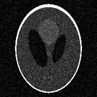
(b)

(c)

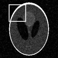
(d)

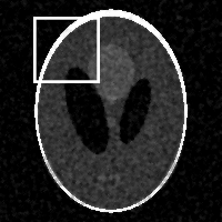
(e)

(f)

(g)

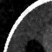
(h)

(i)

(j)

(k)

Figure 3: Comparison of the results of the CFP (4.7) (d), (f) and the ICFP (4.9) (e), (g) and close-ups (h)-(k) of the regions marked in white. From the close-ups, we observe that the ICFP is better suited as a denoising method than the CFP.

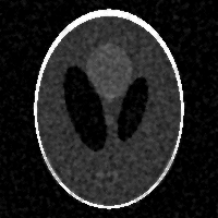
(a) $\alpha=1$

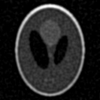
(b) $\alpha=0.1$

Figure 4: Results for varying parameter $\alpha$ (cf. (4.8)). Observe that decreasing $\alpha$ leads to a smoother image.

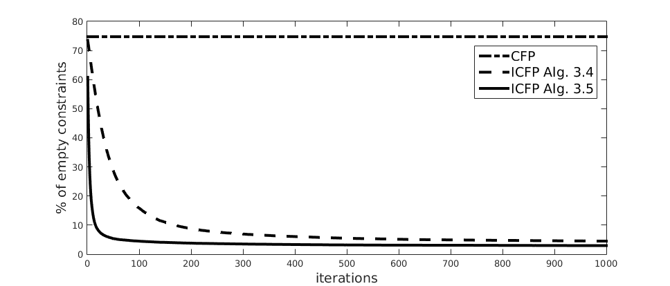
Figure 5: Percentage of empty constraint sets $\cap_{s=1}^{4}C_{s}^{i,j}(X)$, $i=1,2,\dots,{n_{1}}$, $j=1,2,\dots,{n_{2}}$ (inconsistent cases) with $x$ varying during the iterations. We compare the algorithm for the CFP (dash-dotted), and for ICFP Algorithm 3.4 (dashed) and the sequential Algorithm 3.5 (solid). We observe, that for the ICFP, the percentage significantly decreases during the iterations, while for the CFP by definition it is constant.

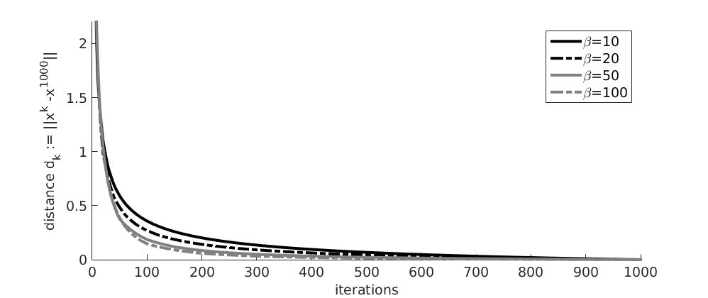
Figure 6: Convergence for different $\beta$-steering sequences with $\beta=10$ (black solid), $20$ (black dashed), $50$ (gray solid) and $100$ (gray dashed) in Algorithm 3.5 applied for smoothing the phantom image. Note that the limit depends on the chosen sequence. We depict $\|X^{k}-X^{1000}\|$, assuming convergence within the first 1000 steps. We conclude that a larger $\beta$ is advantageous for a faster convergence.

5 Summary and further discussion

In this paper we consider the implicit convex feasibility problem (ICFP) where the variable sets are obtained by shifting, rotating and linearly-scaling fixed, closed convex sets. By reformulating the problem as an unconstrained minimization we present two algorithmic schemes for solving the problem, one simultaneous and one sequential. We also comment that other first-order methods can be applied if, for example, the problem is phrased as a variational inequality problem. We illustrate the usefulness of the ICFP as a new modeling technique for imposing constraints on image intensities in image denoising.

Two instances of the ICFP, the wireless sensor network (WSN) positioning problem and the new image denoising approach suggest the applicability potential of the ICFP. In this direction we recall the nonlinear multiple-sets split feasibility problem (NMSSFP) introduced by Li et al. [29] and later by Gibali et al. [23].

In this problem the linear operator $T:\mathbb{R}^{n}\rightarrow\mathbb{R}^{m}$ in the split convex feasibility problem (2.1) is nonlinear and, therefore, the corresponding proximity function is not necessarily convex which means that additional assumptions on $T$ are required, such as differentiability. Within this framework it will be interesting to know, for example, what are the necessary assumptions on $m:\mathbb{R}^{n}\rightarrow\mathbb{R}^{n}$ in Definition 2.4 which will guarantee convergence of our proposed schemes.

Another direction is when the unitary matrices $U_{s}$ are not given in advance but generated via some procedure; for example, given a linear transformation $M:\mathbb{R}^{n}\rightarrow\mathbb{R}^{n\times n}$, such that for all $x\in\mathbb{R}^{n}$, $M(x)=U_{[x]}$ is a unitary matrix. The linearity assumption on $M$ will guarantee that our analysis here will still hold true. For a nonlinear $M$ our present analysis will not hold or, at least, not directly hold.

Acknowledgments. We thank the anonymous referees for their comments and suggestions which helped us improve the paper. The first author’s work was supported by Research Grant No. 2013003 of the United States-Israel Binational Science Foundation (BSF).

References

- [1] F. Aström, G. Baravdish, and M. Felsberg, A tensor variational formulation of gradient energy total variation. In X.-C. Tai, E. Bae, T. Chan, and M. Lysaker, editors, Energy Minimization Methods in Computer Vision and Pattern Recognition, volume 8932 of Lecture Notes in Computer Science, pages 307–320. Springer, 2015.
- [2] J. Baillon and G. Haddad, Quelques propriétés des opérateurs angelbornés et n-cycliquement monotones, Israel Journal of Mathematics 26 (1977), 137–150.
- [3] H. H. Bauschke and J. M. Borwein, On projection algorithms for solving convex feasibility problems, SIAM Review 38 (1996), 367–426.
- [4] D. P. Bertsekas, Nonlinear Programming, Belmont, MA, USA: Athena Scientific, 1995.
- [5] K. Bredies, K. Kunisch, and T. Pock, Total Generalized Variation, SIAM Journal on Imaging Sciences 3(2010), 492–526.
- [6] A. Buades, B. Coll, and J. M. Morel, A review of image denoising algorithms, with a new one, SIAM Journal on Multiscale Modeling and Simulation 4 (2005), 490–530.
- [7] C. Byrne, A unified treatment of some iterative algorithms in signal processing and image reconstruction, Inverse Problems 20 (2004), 103–120.
- [8] C. Byrne, Y. Censor, A. Gibali and S. Reich, The split common null point problem, Journal of Nonlinear and Convex Analysis 13 (2012), 759–775.
- [9] F. Catté, P.-L. Lions, J.-M. Morel, and T. Coll, Image selective smoothing and edge detection by nonlinear diffusion, SIAM Journal on Numerical Analysis 29 (1992), 182–193.
- [10] A. Cegielski, Iterative Methods for Fixed Point Problems in Hilbert Spaces, Springer, Heidelberg, 2012.
- [11] Y. Censor and A. Cegielski, Projection methods: an annotated bibliography of books and reviews, Optimization 64 (2015), 2343–2358.
- [12] Y. Censor, A. R. De Pierro and M. Zaknoon, Steered sequential projections for the inconsistent convex feasibility problem, Nonlinear Analysis: Theory, Methods and Applications 59 (2004), 385–405.
- [13] Y. Censor and T. Elfving , A multiprojection algorithm using Bregman projections in a product space, Numerical Algorithms 8 (1994), 221–239.
- [14] Y. Censor, T. Elfving, N. Kopf and T. Bortfeld, The multiple-sets split feasibility problem and its applications for inverse problems, Inverse Problems 21 (2005), 2071–2084.
- [15] Y. Censor, A. Gibali and S. Reich, Algorithms for the split variational inequality problem, Numerical Algorithms 59 (2012), 301–323.
- [16] S. G. Chang, B. Yu, and M. Vetterli, Adaptive wavelet thresholding for image denoising and compression, IEEE Transactions on Image Processing 9 (2000), 1532–1546.
- [17] K. Dabov, A. Foi, V. Katkovnik, and K. Egiazarian, Image denoising by sparse 3-d transform-domain collaborative filtering, IEEE Transactions on Image Processing, 16 (2007), 2080–2095.
- [18] Z. O. Dolidze, On convergence of an analog of the gradient method, Ekonomika i Matematicheskie Metody 20 (1984), 755–758.
- [19] V. Estellers, S. Soato, and X. Bresson, Adaptive regularization with the structure tensor, IEEE Transactions on Image Processing, 24 (2015), 1777–1790.
- [20] M. R. Gholami, Positioning Algorithms for Wireless Sensor Networks, Licentiate Thesis 2011, Chalmers University of Technology, Gothenburg, Sweden.
- [21] M. R. Gholami, L. Tetruashvili, E. G. Ström and Y. Censor, Cooperative wireless sensor network positioning via implicit convex feasibility, IEEE Transactions on Signal Processing 61 (2013), 5830–5840.
- [22] M. R. Gholami and H. Wymeersch and E. G. Ström and M. Rydström, Wireless network positioning as a convex feasibility problem, EURASIP Journal on Wireless Communications and Networking 161 (2011), 1–15.
- [23] A. Gibali, K.-H. Küfer and P. Süss, Successive linear programing approach for solving the nonlinear split feasibility problem, Journal of Nonlinear and Convex Analysis 15 (2014), 345–353.
- [24] K. Goebel and S. Reich, Uniform Convexity, Hyperbolic Geometry, and Nonexpansive Mappings, Marcel Dekker, New York and Basel, 1984.
- [25] S. Kindermann, S. Osher, and P. Jones, Deblurring and denoising of images by nonlocal functionals, SIAM-Multiscale Modeling and Simulation, 4 (2005), 1091–1115.
- [26] G. M. Korpelevich, The extragradient method for finding saddle points and other problems, Ekonomika i Matematicheskie Metody 12 (1976), 747–756.
- [27] S. Lefkimmiatis, A. Roussos, P. Maragos, and M. Unser, Structure tensor total variation, SIAM Journal on Imaging Sciences 8 (2015), 1090–1122.
- [28] F. Lenzen and J. Berger, Solution-driven adaptive total variation regularization, In J.-F. Aujol, M. Nikolova, and N. Papadakis, editors, Proceedings of SSVM 2015, volume 9087 of LNCS, pages 203–215, 2015.
- [29] Z. Li, D. Han and W. Zhang, A self-adaptive projection-type method for nonlinear multiple-sets split feasibility problem, Inverse Problems in Science and Engineering 21 (2013), 155–170.
- [30] G. Lopez, V. Martin-Marquez, F. Wang and H.-K Xu, Solving the split feasibility problem without prior knowledge of matrix norms, Inverse Problems 28:085004 (2012).
- [31] E. Masad and S. Reich, A note on the multiple-set split convex feasibility problem in Hilbert space, Journal of Nonlinear and Convex Analysis 8 (2007), 367–371.
- [32] C. Popa, Projection Algorithms - Classical Results and Developments: Applications to Image Reconstruction, Lambert Academic Publishing - AV Akademikerverlag GmbH & Co. KG, Saarbrücken, Germany, 2012.
- [33] L. Rudin, S. Osher, and E. Fatemi, Nonlinear total variation based noise removal algorithms, Physica D 60 (1992), 259–268.
- [34] O. Scherzer, M. Grasmair, H. Grossauer, M. Haltmeier, and F. Lenzen, Variational Methods in Imaging, Springer, 2009.
- [35] S. Setzer, G. Steidl, and T. Teuber, Infimal convolution regularizations with discrete l1-type functionals, Communications in Mathematical Sciences 9 (2011), 797–872.
- [36] Y. Shehu, G. Cai and O. S. Iyiola, Iterative approximation of solutions for proximal split feasibility problems, Fixed Point Theory and Applications, 2015:123 (2015).
- [37] Z. Wang, A. Bovik, H. Sheikh, and E. Simoncelli, Image quality assessment: from error visibility to structural similarity, IEEE Transactions on Image Processing 13 (2004), 600–612.
- [38] J. Weickert, Anisotropic Diffusion in Image Processing, Teubner Verlag, 1998.
- [39] Y. Xiao, Y. Censor, D. Michalski and J.M. Galvin, The least-intensity feasible solution for aperture-based inverse planning in radiation therapy, Annals of Operations Research 119 (2003), 183–203.