Conservative Integrators for a Toy Model of Weak Turbulence

Abstract.

Weak turbulence is a phenomenon by which a system generically transfers energy from low to high wave numbers, while persisting for all finite time. It has been conjectured by Bourgain and others that the 2D defocusing nonlinear Schrödinger equation (NLS) on the torus has this dynamic, and several analytical and numerical studies have worked towards addressing this point.

In the process of studying the conjecture, Colliander, Keel, Staffilani, Takaoka, and Tao introduced a “toy model” dynamical system as an approximation of NLS, which has been subsequently studied numerically. In this work, we formulate and examine several numerical schemes for integrating this model equation. The model has two invariants, and our schemes aim to conserve at least one of them. We prove convergence in some cases, and our numerical studies show that the schemes compare favorably to others, such as Trapezoidal Rule and fixed step fourth order Runge-Kutta. The preservation of the invariants is particularly important in the study of weak turbulence as the energy transfer tends to occur on long time scales.

1. Introduction

In [9], the 2D, defocusing, cubic, toroidal nonlinear Schrödinger equation (NLS),

(1.1) $$iu_{t}+\Delta u-|u|^{2}u=0,\ \ u(0,x)=u_{0}(x)\ \text{for}\ x\in\mathbb{T}^{2},$$

was approximated by a “Toy Model System” given by the equation

(1.2) $$-i\dot{b}_{j}=-\left|b_{j}\right|^{2}b_{j}+2b_{j-1}^{2}\overline{b}_{j}+2b_{j+1}^{2}\overline{b}_{j},\quad\text{for $j=1\ldots N$}$$

with boundary conditions

(1.3) $$b_{0}(t)=b_{N+1}(t)=0.$$

Subject to these boundary conditions, (1.2) conserves $\ell^{2}$,

(1.4) $$\mathcal{M}[\mathbf{b}(t)]=\sum_{j=1}^{N}|b_{j}(t)|^{2},$$

and the Hamiltonian

(1.5) $$\mathcal{H}[\mathbf{b}(t)]=\sum_{j=1}^{N}\left(\frac{1}{4}|b_{j}(t)|^{4}-\text{Re}(\bar{b}_{j}(t)^{2}b_{j-1}(t)^{2})\right).$$

Indeed, the flow of (1.2) can be expressed as

(1.6) $$i\dot{b}_{j}=2\frac{\partial\mathcal{H}[\mathbf{b}]}{\partial\bar{b}_{j}}.$$

In this way, we can interpret (1.2) as a Hamiltonian system of nonlinearly and degenerately coupled oscillators.

1.1. Weak Turbulence

Roughly, $|b_{j}(t)|^{2}$ measures the spectral energy of $u$, the solution to (1.1), on a set of wave numbers, $\Lambda_{j}$. The sets $\Lambda_{j}$ are tailored to have the property that the largest wave number in $\Lambda_{j+1}$ exceeds the largest wave number in $\Lambda_{j}$. Thus, larger values of $|b_{j}|^{2}$ at larger values of $j$ correspond to more energy of $u$ in higher wave numbers.

The motivation for the approximation of (1.1) by (1.2) was to explore a long-standing hypothesis that (1.1) could capture the phenomenon of weak turbulence; see [4, 13, 9] and references therein. Loosely speaking, a weakly turbulent system exists globally in time, yet continuously propagates energy to ever higher frequencies. Thus, the norms tend to infinity, but are finite at all finite times. Another model equation for weak turbulence was formulated by Majda, McLaughlin, and Tabak, [6, 5, 7, 13, 19, 24].

In [9], the authors proved that, given $N$, they could construct a solution of (1.2) which would propagate energy from $|b_{j}|^{2}$ at low index to high index $j$. This corresponds to a transfer of energy in (1.1), and, subject to rigorous analysis of the approximation, demonstrated that such energy cascades were present. However, this did not show that energy transfer in (1.1) was a generic phenomenon, an essential feature of weak turbulence. Analysis of this problem has continued in the recent works [15, 17]. Separately, in [10, 18], (1.2) was numerically simulated and observed to have such energy transfers for a variety of initial conditions for the lifespan of the simulations.

1.2. Relation to Previous Work

In [10, 18], (1.2) was integrated using high order, adaptive, Runge-Kutta (RK) integrators. While the RK integrators gave high quality results for the duration of the simulations, they are unable to exactly conserve either of the two invariants. At the same time, the energy transfer in the toy model system is slow, requiring integration out to long times. Thus, the RK integrators require significant computational effort to observe weak turbulence – small steps are needed for accuracy, but the phenomenological time of integration is long.

Given the interest in (1.2), the goal of this work is to present conservative methods that may aid in statistical studies of weak turbulence and other long time integration problems. The methods presented here are second order in the time step, $\Delta t$. In numerical experiments, we observe that comparatively large time steps can be taken with these schemes for exploring weak turbulence. While pointwise accuracy is lost with large $\Delta{t}$, the average energy transfer appears robust. In contrast, fixed time step RK schemes will, eventually, cease to provide accurate output.

A variety of strategies have been proposed for integrating Hamiltonian systems so as to preserve the invariants of the equations, including splitting methods, projection methods, symplectic methods, and the average vector field method, [14, 16, 8]. In this work, we explore some conservative discretizations of (1.2) which preserve either (1.4) or (1.5), including implicit midpoint. Some appear to be ad hoc and not from one of the aforementioned known discretization strategies, instead taking their inspiration from known discretizations of NLS, [21, 12]. We also direct the reader to the recent work in [23], where the author tested an explicit symplectic integration scheme on (1.2) with a small number of nodes, $N=5$.

1.3. Outline

Our paper is organized as follows. In Section 2 we formulate out schemes. Next, in Section 3, we prove a number of results on the the integrators. Numerical simulations are presented in Section 4, and we discuss our results in Section 5.

2. Conservative Integrators

In this section, we formulate our discretizations and prove that they conserve the relevant invariant, under a solvability assumption. These schemes are all symmetric, but the nonlinear terms are treated differently in each case. Since the dependent variables of (1.2) are nonlinearly and degenerately coupled, formulating a conservative scheme is nontrivial. This is contrast to NLS, where the spatial coupling, the analog of the lattice site coupling of (1.2), is linear.

Before stating the schemes, we introduce some notation. Throughout, we assume the time step, $\Delta{t}$, is constant. We will solve at times $t_{n}=n\Delta t$, and our approximation will be $\mathbf{b}_{n}\approx\mathbf{b}(t_{n})$, with components $b_{j,n}\approx b_{j}(t_{n})$. We define the following linear and nonlinear averages as:

(2.1a) $$b_{j,n} \approx b_{j}(t_{n})$$

(2.1b) $$b_{j,n+1/2} =\tfrac{1}{2}\left(b_{j,n}+b_{j,n+1}\right)$$

(2.1c) $$b_{j,n+1/2}^{2} =\left[\tfrac{1}{2}\left(b_{j,n}+b_{j,n+1}\right)\right]^{2}$$

(2.1d) $$(b^{2})_{j,n+1/2} =\tfrac{1}{2}\left(b_{j,n}^{2}+b_{j,n+1}^{2}\right)$$

(2.1e) $$\left|b\right|^{2}_{j,n+1/2} =\tfrac{1}{2}\left(\left|b_{j,n}\right|^{2}+\left|b_{j,n+1}\right|^{2}\right)$$

Using this notation, the trapezoidal method corresponds to

(2.2) $$\begin{split}{\bf b}_{n+1}&={\bf b}_{n}+\Delta{t}{\bf F}^{\rm Trap}(\mathbf{b}_{n},\mathbf{b}_{n+1};\Delta{t})\\ F_{j}^{\rm Trap}&=\frac{i}{2}\left[-\left|b_{j,n}\right|^{2}b_{j,n}+2\overline{b}_{j,n}(b_{j-1,n}^{2}+b_{j+1,n}^{2})\right]\\ &\quad+\frac{i}{2}\left[-\left|b_{j,n+1}\right|^{2}b_{j,n+1}+2\overline{b}_{j,n+1}(b_{j-1,n+1}^{2}+b_{j+1,n+1}^{2})\right]\end{split}$$

while the implicit midpoint method corresponds to

(2.3) $$\begin{split}{\bf b}_{n+1}&={\bf b}_{n}+\Delta{t}{\bf F}^{\rm Midpt}(\mathbf{b}_{n},\mathbf{b}_{n+1};\Delta{t})\\ F_{j}^{\rm Midpt}&=-i|b_{j,n+1/2}|^{2}b_{j,n+1/2}+2i\bar{b}_{j,n+1/2}(b_{j-1,n+1/2}^{2}+b_{j+1,n+1/2}^{2})\end{split}$$

While the results we present in this section are for the Dirichlet type boundary conditions (1.3), it can be verified that they also apply to the periodic boundary condition case,

(2.4) $$b_{0}(t)=b_{N}(t),\quad b_{N+1}(t)=b_{1}(t).$$

2.1. Mass Preserving Integrators

We first note that the implicit midpoint method, given by (2.3), conserves (1.4):

Proposition 2.1.

Assume that the nonlinear algebraic system in (2.3) can be solved exactly for $b_{j,n+1}$. Then (1.4) is exactly conserved.

Proof.

This is a consequence of the mass invariant being quadratic which can be expressed as

$$\mathcal{M}[\mathbf{b}]=\left\langle\mathbf{b},\mathbf{b}\right\rangle={\mathrm{Re}}\sum_{j=1}^{N}(b_{j}\bar{b}_{j}).$$

By virtue of conservation of mass,

$$\left\langle\mathbf{b},\frac{d\mathbf{b}}{dt}\right\rangle={\mathrm{Re}}\sum_{j=1}^{N}\bar{b}_{j}\frac{db_{j}}{dt}=0.$$

The conservation for the scheme, being symplectic, then follows from a result due to Cooper, [11, 16]. ∎

The following modified midpoint method also preserves mass:

(2.5) $$\begin{split}9\mathbf{b}_{n+1}&=\mathbf{b}_{n}+\Delta{t}{\bf F}^{\rm Mass}(\mathbf{b}_{n},\mathbf{b}_{n+1};\Delta{t})\\ F_{j}^{\rm Mass}&=-i\left|b\right|^{2}_{j,n+1/2}b_{j,n+1/2}+2i\bar{b}_{j,n+1/2}\left(b_{j+1,n+1/2}^{2}+b_{j-1,n+1/2}^{2}\right)\end{split}$$

Note the difference in the self-interaction schemes of (2.5) and (2.3),

$$-\left|b\right|^{2}_{j,n+1/2}b_{j,n+1/2}\quad\text{vs}\quad-|b_{j,n+1/2}|^{2}b_{j,n+1/2}.$$

This treatment of the nonlinear term in (2.5) is modeled upon the analogous expression for some conservative NLS schemes, [21, 12].

Proposition 2.2.

Assume that the nonlinear algebraic system in (2.5) can be solved exactly for $b_{j,n+1}$. Then (1.4) is exactly conserved.

Proof.

Multiplying the $j$- th equation of(2.5) by $\bar{b}_{j,n+1/2}$, we have

$$\begin{split}&{\left|b_{j,n+1}\right|^{2}-\left|b_{j,n}\right|^{2}-b_{j,n}\bar{b}_{j,n+1}+\bar{b}_{j,n}b_{j,n+1}}\\ &\quad=-2i\Delta t\left|b\right|_{j,n+1/2}^{2}\left|b_{j,n+1/2}\right|^{2}+4i\Delta t\bar{b}_{j,n+1/2}^{2}\left(b_{j+1,n+1/2}^{2}+b_{j-1,n+1/2}^{2}\right)\end{split}$$

Taking the real part of this equation, we obtain

$$\begin{split}&\left|b_{j,n+1}\right|^{2}-\left|b_{j,n}\right|^{2}\\ &\quad=4\Delta t{\mathrm{Re}}\left\{i\bar{b}_{j,n+1/2}^{2}b_{j+1,n+1/2}^{2}+i\bar{b}_{j,n+1/2}^{2}b_{j-1,n+1/2}^{2}\right\},\end{split}$$

and summing over $j$,

$$\begin{split}&\sum_{j=1}^{N}\left|b_{j,n+1}\right|^{2}-\left|b_{j,n}\right|^{2}\\ &\quad=4\Delta t\sum_{j=1}^{N}{\mathrm{Re}}\left\{i\bar{b}_{j,n+1/2}^{2}b_{j+1,n+1/2}^{2}+i\bar{b}_{j,n+1/2}^{2}b_{j-1,n+1/2}^{2}\right\}.\end{split}$$

Shifting indices on the second term and using that $b_{0}=b_{N+1}=0$, we have

$$\begin{split}&\sum_{j=1}^{N}{\mathrm{Re}}\left\{i\bar{b}_{j,n+1/2}^{2}b_{j+1,n+1/2}^{2}+i\bar{b}_{j,n+1/2}^{2}b_{j-1,n+1/2}^{2}\right\}\\ &\quad=\sum_{j=1}^{N}{\mathrm{Re}}\left\{i\bar{b}_{j,n+1/2}^{2}b_{j+1,n+1/2}^{2}+i\bar{b}_{j+1,n+1/2}^{2}b_{j,n+1/2}^{2}\right\}\\ &\quad=\sum_{j=1}^{N}{\mathrm{Re}}\left\{i2{\mathrm{Re}}\left(\bar{b}_{j,n+1/2}^{2}b_{j+1,n+1/2}^{2}\right)\right\}=0.\end{split}$$

Therefore,

$$\sum_{j=1}^{N}\left|b_{j,n+1}\right|^{2}=\sum_{j=1}^{N}\left|b_{j,n}\right|^{2}.$$

∎

2.2. Hamiltonian Preserving Integrator

One numerical scheme which exactly preserves the energy, (1.5), is:

(2.6) $$\begin{split}\mathbf{b}_{n+1}&=\mathbf{b}_{n}+\Delta{t}\mathbf{F}^{\rm Eng}(\mathbf{b}_{n},\mathbf{b}_{n+1};\Delta{t})\\ F^{\rm Eng}_{j}&=-i\left|b\right|^{2}_{j,n+1/2}b_{j,n+1/2}+2i\bar{b}_{j,n+1/2}\left[(b^{2})_{j+1,n+1/2}+(b^{2})_{j-1,n+1/2}\right]\end{split}$$

Note how the $j$-$j+1$ and $j$-$j-1$ interaction terms are handled differently than in (2.2), (2.3), and (2.5). This scheme, which we show to exactly preserve (1.5), appears to be ad hoc, and is not based upon a known methodology, such as average vector field, for deriving schemes which conserve the energy.

Proposition 2.3.

Assume that the nonlinear algebraic system in (2.6) can be solved exactly for $b_{j,n+1}$. Then (1.5) is exactly conserved.

Proof.

Multiplying the $j$-th equation of (2.6) by $\bar{b}_{j,n+1}-\bar{b}_{j,n}$, we have

$$\begin{split}\left|b_{j,n+1}-b_{j,n}\right|^{2}&=-i\Delta t\left|b\right|^{2}_{j,n+1/2}b_{j,n+1/2}(\bar{b}_{j,n+1}-\bar{b}_{j,n})\\ &\quad+2i\Delta t\bar{b}_{j,n+1/2}\left[(b^{2})_{j+1,n+1/2}+(b^{2})_{j-1,n+1/2}\right](\bar{b}_{j,n+1}-\bar{b}_{j,n})\\ &=-i\frac{\Delta t}{4}(\left|b_{j,n+1}\right|^{4}-\left|b_{j,n}\right|^{4})+\Delta t\left|b\right|^{2}_{j,n+1/2}{\mathrm{Im}}(b_{j,n}\bar{b}_{j,n+1})\\ &\quad+i\Delta t\left[(b^{2})_{j+1,n+1/2}+(b^{2})_{j-1,n+1/2}\right]\left[\bar{b}^{2}_{j,n+1}-\bar{b}^{2}_{j,n}\right]\end{split}$$

Taking the imaginary parts and dividing out by $\Delta t$,

(2.7) $$\begin{split}0&=\tfrac{1}{4}(\left|b_{j,n+1}\right|^{4}-\left|b_{j,n}\right|^{4})\\ &\quad-{\mathrm{Im}}\left\{i\left[(b^{2})_{j+1,n+1/2}+(b^{2})_{j-1,n+1/2}\right]\left[\bar{b}^{2}_{j,n+1}-\bar{b}^{2}_{j,n}\right]\right\}\end{split}$$

Examining the second term,

$$\begin{split}&\left[(b^{2})_{j+1,n+1/2}+(b^{2})_{j-1,n+1/2}\right]\left[\bar{b}^{2}_{j,n+1}-\bar{b}^{2}_{j,n}\right]\\ &=\frac{1}{2}\left[b^{2}_{j+1,n+1}\bar{b}^{2}_{j,n+1}-b^{2}_{j+1,n+1}\bar{b}^{2}_{j,n}+b^{2}_{j+1,n}\bar{b}^{2}_{j,n+1}-b^{2}_{j+1,n}\bar{b}^{2}_{j,n}\right.\\ &\quad\left.+b^{2}_{j-1,n+1}\bar{b}^{2}_{j,n+1}-b^{2}_{j-1,n+1}\bar{b}^{2}_{j,n}+b^{2}_{j-1,n}\bar{b}^{2}_{j,n+1}-b^{2}_{j-1,n}\bar{b}^{2}_{j,n}\right]\end{split}$$

Summing from $j=1,\ldots,N$, and using $b_{0}=b_{N+1}=0$ to shift indices,

$$\begin{split}&\sum_{j=1}^{N}\frac{1}{2}\left[b^{2}_{j+1,n+1}\bar{b}^{2}_{j,n+1}-b^{2}_{j+1,n+1}\bar{b}^{2}_{j,n}+b^{2}_{j+1,n}\bar{b}^{2}_{j,n+1}-b^{2}_{j+1,n}\bar{b}^{2}_{j,n}\right.\\ &\quad\left.+b^{2}_{j-1,n+1}\bar{b}^{2}_{j,n+1}-b^{2}_{j-1,n+1}\bar{b}^{2}_{j,n}+b^{2}_{j-1,n}\bar{b}^{2}_{j,n+1}-b^{2}_{j-1,n}\bar{b}^{2}_{j,n}\right]\\ &=\sum_{j=1}^{N}\frac{1}{2}\left[b^{2}_{j+1,n+1}\bar{b}^{2}_{j,n+1}-b^{2}_{j+1,n+1}\bar{b}^{2}_{j,n}+b^{2}_{j+1,n}\bar{b}^{2}_{j,n+1}-b^{2}_{j+1,n}\bar{b}^{2}_{j,n}\right.\\ &\quad\left.+b^{2}_{j,n+1}\bar{b}^{2}_{j+1,n+1}-b^{2}_{j,n+1}\bar{b}^{2}_{j+1,n}+b^{2}_{j,n}\bar{b}^{2}_{j+1,n+1}-b^{2}_{j,n}\bar{b}^{2}_{j+1,n}\right]\\ &=\sum_{j=1}{\mathrm{Re}}\left[b^{2}_{j+1,n+1}\bar{b}^{2}_{j,n+1}-b^{2}_{j+1,n}\bar{b}^{2}_{j,n}\right]+i{\mathrm{Im}}\left[b^{2}_{j,n}\bar{b}^{2}_{j+1,n+1}+b^{2}_{j+1,n}\bar{b}^{2}_{j,n+1}\right]\end{split}$$

Summing (2.7) over $j$, and using the preceding calculation,

$$0=\sum_{j=1}^{N}\frac{1}{4}(\left|b_{j,n+1}\right|^{4}-\left|b_{j,n}\right|^{4})-\sum_{j=1}^{N}{\mathrm{Re}}\left[b^{2}_{j+1,n+1}\bar{b}^{2}_{j,n+1}-b^{2}_{j+1,n}\bar{b}^{2}_{j,n}\right]$$

Therefore,

$$\sum_{j}\frac{1}{4}\left|b_{j,n+1}\right|^{4}-{\mathrm{Re}}(b^{2}_{j+1,n+1}\bar{b}^{2}_{j,n+1})=\sum_{j}\frac{1}{4}\left|b_{j,n}\right|^{4}-{\mathrm{Re}}(b^{2}_{j+1,n}\bar{b}^{2}_{j,n})$$

Shifting indices and using $b_{0}=b_{N+1}=0$ again yields the conservation of the energy, (1.5), in the discretized evolution.

Again, a similar calculation holds in the case of periodic boundary conditions, $b_{0}=b_{N}$ and $b_{N+1}=b_{1}$. ∎

3. Convergence of Integrators

In this section we examine the convergence of our integrators. We provide a complete proof in the case of mass preserving schemes, as it gives a priori estimates on $b_{j,n}$ at all $j$ and $n$. We can also provide a partial proof for the energy preserving scheme. We proceed in the following steps. First we prove results on the solvability of the nonlinear algebraic systems. Next we establish stability and consistency. Finally, we prove convergence.

3.1. Solvability

We prove solvability via the implicit function theorem.

Lemma 3.1.

Given $\mathbf{b}_{n}$ and one of the three schemes, there exists $\Delta{t}_{1}>0$, depending on $\|\mathbf{b}_{n}\|_{2}$, such that for all $\Delta{t}\leq\Delta{t}_{1}$, a unique solution, $\mathbf{b}_{n+1}$, exists. Moreover, as a function of $\Delta{t}$, $\mathbf{b}_{n+1}$ is $C^{1}$.

Proof.

We frame this in terms of real and imaginary parts, with $\mathbf{b}=\mathbf{u}+i\mathbf{v}$, and $\mathbf{u},\mathbf{v}\in\mathbb{R}^{N}$. Define the function $\mathcal{F}:\mathbb{R}^{2N}\times\mathbb{R}\to\mathbb{R}^{2N}$ as follows.

(3.1) $$\mathcal{F}(\mathbf{u},\mathbf{v},\Delta{t};\mathbf{b}_{n})=\begin{pmatrix}\mathbf{u}\\ \mathbf{v}\end{pmatrix}-\begin{pmatrix}{\mathrm{Re}}\mathbf{b}_{n}\\ {\mathrm{Im}}\mathbf{b}_{n}\end{pmatrix}-\Delta{t}\begin{pmatrix}{\mathrm{Re}}\mathbf{F}(\mathbf{b}_{n},\mathbf{u}+i\mathbf{v};\Delta{t})\\ {\mathrm{Im}}\mathbf{F}(\mathbf{b}_{n},\mathbf{u}+i\mathbf{v};\Delta{t})\end{pmatrix}$$

Notice that ${\mathrm{Re}}\mathbf{F}(\mathbf{b}_{n},\mathbf{u}+i\mathbf{v};\Delta{t})$ and ${\mathrm{Im}}\mathbf{F}(\mathbf{b}_{n},\mathbf{u}+i\mathbf{v};\Delta{t})$ are cubic in the components of $\mathbf{u}$ and $\mathbf{v}$. Taking a gradient of the above expression in $(\mathbf{u},\mathbf{v})$,

(3.2) $$\nabla_{\mathbf{u},\mathbf{v}}\mathcal{F}=I-\Delta{t}\nabla_{\mathbf{u},\mathbf{v}}\begin{pmatrix}{\mathrm{Re}}\mathbf{F}(\mathbf{b}_{n},\mathbf{u}+i\mathbf{v};\Delta{t})\\ {\mathrm{Im}}\mathbf{F}(\mathbf{b}_{n},\mathbf{u}+i\mathbf{v};\Delta{t})\end{pmatrix}$$

At $\Delta{t}=0$,the solution is simply $\mathbf{u}={\mathrm{Re}}\mathbf{b}_{n}$ and $\mathbf{v}={\mathrm{Im}}\mathbf{b}_{n}$. Furthermore,

$$\left.\nabla_{\mathbf{u},\mathbf{v}}\mathcal{F}\right|_{\begin{subarray}{c}\mathbf{u}=\mathbf{u}_{n}\\ \mathbf{v}=\mathbf{v}_{n}\\ \Delta{t}=0\end{subarray}}=I.$$

Therefore the implicit function theorem applies and there exists a positive interval of $\Delta{t}$ values for which we can compute $\Delta{t}\mapsto(\mathbf{u},\mathbf{v})\mapsto\mathbf{b}=\mathbf{u}+i\mathbf{v}$.

That $\Delta{t}_{1}$ is controlled by $\|\mathbf{b}_{n}\|_{2}$ follows from our use of the $\ell^{2}$ topology in our application of the implicit function theorem, [22].

∎

Corollary 3.2.

Given an initial condition, $\mathbf{b}_{0}$, there exists a $\Delta{t}_{1}$ such that for any fixed $\Delta{t}\leq\Delta{t}_{1}$, the mass preserving schemes can always be solved.

Proof.

By Lemma 3.1, we can find a $\Delta{t}_{1}$ to compute $\mathbf{b}_{1}$ for an admissible $\Delta{t}$. Since the mass schemes conserve $\ell_{2}$, $\mathbf{b}_{1}$ has the same $\ell_{2}$ norm as $\mathbf{b}_{0}$. Since $\Delta{t}_{1}$ only depends on the magnitude of this norm, it remains an applicable value for computing $\mathbf{b}_{2}$, which can be computed at the same $\Delta{t}$. By induction this can be carried on to any iterate. ∎

Remark 3.3.

Since the energy invariant (1.5) does not provide a priori bounds on a norm, we are unable to show global persistence of the energy preserving scheme.

3.2. Stability

Obviously, our schemes have the desired stability property owing to the smoothness of the $\mathbf{F}$ functions in all cases:

Lemma 3.4.

For each integration scheme, there exists a polynomial $\Pi$, with positive coefficients, such that for all $\mathbf{u},\mathbf{v},\tilde{\mathbf{u}},\tilde{\mathbf{v}}\in\mathbb{C}^{N}$:

$$\|\mathbf{F}(\mathbf{u},\mathbf{v})-\mathbf{F}(\tilde{\mathbf{u}},\tilde{\mathbf{v}})\|\leq\Pi(\|\mathbf{u}\|_{2},\|\mathbf{v}\|_{2},\|\tilde{\mathbf{u}}\|_{2},\|\tilde{\mathbf{v}}\|_{2})(\|\mathbf{u}-\tilde{\mathbf{u}}\|+\|\mathbf{v}-\tilde{\mathbf{v}}\|)$$

Proof.

Since the components of $\mathbf{F}$ are cubic in their arguments and the $\ell^{2}$ norm gives pointwise control, the result is immediate. Each scheme will have a different polynomial.

∎

3.3. Consistency

Before obtaining the consistency result, we state a lemma about the solution to (1.2).

Theorem 3.5.

Let $\mathbf{b}(t)$ be the solution to (1.2) for initial condition $\mathbf{b}(0)$. Then $\mathbf{b}(t)$ is a $C^{\infty}$ and a global in time such that for any $k$, there is a polynomial, $\Pi_{k}$, with positive coefficients such that

(3.3) $$\left\|\frac{d^{k}\mathbf{b}}{dt^{k}}\right\|_{2}\leq\Pi_{k}(\left\|\mathbf{b}(0)\right\|_{2})$$

Proof.

Since (1.2) has a righthand side which is polynomial in $b_{j}$ and $\bar{b}_{j}$, a $C^{1}$ local in time solution exists. Since it conserves $\ell^{2}$, it will in fact be global. By a bootstrap argument, it will also be $C^{\infty}$. The polynomial bound in terms of the data can then be obtained by induction. ∎

Lemma 3.6.

For any of the conservative schemes, the local truncation error is

$$\|\mathbf{b}(t_{n+1})-\mathbf{b}(t_{n})-\Delta{t}\mathbf{F}(\mathbf{b}(t_{n}),\mathbf{b}(t_{n+1}))\|\leq C\Delta{t}^{3},$$

and the constant $C$ only depends on $\|\mathbf{b}(0)\|_{2}$.

Proof.

We prove this in the case of the mass conserving scheme (2.5). The proofs for implicit midpoint and the energy preserving scheme are similar.

Substituting $\mathbf{b}(t)$ into (2.5),

(3.4) $$\begin{split}\tfrac{i}{\Delta t}(b_{j}(t_{n+1})-b_{j}(t_{n}))-&\tfrac{1}{4}(|b_{j}(t_{n})|^{2}+|b_{j}(t_{n+1})|^{2})(b_{j}(t_{n})+b_{j}(t_{n+1}))\\ \quad+\tfrac{1}{4}(\bar{b}_{j}(t_{n})+\bar{b}_{j}(t_{n+1}))&\left[(b_{j+1}(t_{n})+b_{j+1}(t_{n+1}))^{2}\right.\\ &\quad+\left.(b_{j-1}(t_{n})+b_{j-1}(t_{n+1}))^{2}\right],\end{split}$$

and Taylor expanding about $\Delta{t}=0$,

(3.5) $$\tfrac{i}{\Delta t}(b_{j}(t_{n+1})-b_{j}(t_{n}))=i\dot{b}_{j}+\tfrac{i}{2}\ddot{b}_{j}\Delta{t}+\operatorname{O}(\Delta{t}^{2})$$

(3.6) $$\begin{split}&-\tfrac{1}{4}(|b_{j}(t_{n})|^{2}+|b_{j}(t_{n+1})|^{2})(b_{j}(t_{n})+b_{j}(t_{n+1}))\\ &=-|b_{j}|^{2}b_{j}+\Delta{t}\left[-\tfrac{1}{2}(\bar{b}_{j}\dot{b}_{j}+b_{j}\dot{\bar{b}}_{j})b_{j}-\tfrac{1}{2}|b_{j}|^{2}\dot{b}_{j}\right]+\operatorname{O}(\Delta{t}^{2})\end{split}$$

(3.7) $$\begin{split}&\tfrac{1}{4}(\bar{b}_{j}(t_{n})+\bar{b}_{j}(t_{n+1}))\left[(b_{j+1}(t_{n})+b_{j+1}(t_{n+1}))^{2}+(b_{j-1}(t_{n})+b_{j-1}(t_{n+1}))^{2}\right]\\ &=2\bar{b}_{j}(b_{j+1}^{2}+b_{j-1}^{2})+\Delta{t}\left[\dot{\bar{b}}_{j}(b_{j+1}^{2}+b_{j-1})^{2}+2\bar{b}_{j}(b_{j+1}\dot{b}_{j+1}+b_{j-1}\dot{b}_{j-1})\right]\\ &\quad+\operatorname{O}(\Delta{t}^{2})\end{split}$$

In the above three expressions, we have suppressed the $t_{n}$ dependence in the terms on the righthand side. The $\operatorname{O}(\Delta{t}^{2})$ expressions reflect the remainder terms from the Taylor expansion, which are a priori bounded by Theorem 3.5. Substituting back into (3.4), and writing the equation in terms of $\mathbf{b}(t_{n+1})-\mathbf{b}(t_{n})$ yields the result.

∎

3.4. Convergence

The above consistency and stability results allow us to prove, for the mass preserving schemes:

Theorem 3.7.

Given an initial condition $\mathbf{b}(0)$, for either of the mass conserving schemes, there exists a $\Delta{t}_{\star}$, $K>0$ and $C>0$, such that for all $\Delta{t}\leq\Delta{t}_{\star}$ and all $n$, the error is

(3.8) $$\|\mathbf{b}_{n}-\mathbf{b}(t_{n})\|_{2}\leq C(e^{Kt_{n}}-1)\Delta{t}^{2}$$

Proof.

As the proof is standard, we omit the details. We note that our above result holds for any $n$ by virtue of the conservation of $\ell^{2}$, which gives uniform in $n$ estimates of all constants from the stability and consistency estimates.

∎

Remark 3.8.

If an a priori bound were available for the energy preserving scheme, the analog of Theorem 3.7 would hold for it.

4. Numerical Results

In this section, we explore our methods, and compare them to others. Throughout, we make use of the Portable, Extensible Tookit for Scientific Computation (PETSc), [1, 2, 3], which contains Crank-Nicolson (Trapezoidal Rule), Implicit Midpoint, and Runge-Kutta 4 (RK4) as subroutines. As both linear and nonlinear solvers are required, for these methods, we compute with:

• An absolute tolerance of $10^{-50}$, such that the nonlinear solver terminates at step $k$ if the norm of the residual, $\|\mathbf{r}^{(k)}\|$, falls beneath this value.

• A relative tolerance of $10^{-15}$, such that the nonlinear solver terminates at step $k$ if the norm of the residual relative to the initial residual, $\|\mathbf{r}^{(k)}\|/\|\mathbf{r}^{(0)}\|$, falls beneath this value.

• A step tolerance of $10^{-15}$ such that the nonlinear solver terminates at step $k$ if the norm of the step relative to the norm of the approximate solution, $\|\Delta\mathbf{b}^{(k)}\|/\|\mathbf{b}^{(k)}\|$, falls beneath this value.

These settings mitigate the error due to the nonlinear solvers allowing for a direct examination of the impact of $\Delta{t}$. The nonlinear solvers typically terminate due to either the relative norm or the step size becoming small.

We also compare against a Projection method,

(4.1) $$\mathbf{b}_{n+1}=P(\underbrace{\mathbf{b}_{n}+\Delta{t}\mathbf{F}^{\rm RK4}(\mathbf{b}_{n};\Delta{t})}_{\equiv\mathbf{b}_{n+1}^{\rm RK4}};\mathcal{M}_{0},\mathcal{H}_{0}).$$

Here, a candidate solution for time step $n+1$ is produced with RK4, and the projector finds an element of $\left\{\mathbf{b}\in\mathbb{C}^{N}\mid\mathcal{M}[\mathbf{b}]=\mathcal{M}_{0},\quad\mathcal{H}[\mathbf{b}]=\mathcal{H}_{0}\right\}$, closest to ${\mathbf{b}_{n+1}^{\rm RK4}}$ with respect to the 2-norm. Following, [16], this is approximated by finding Lagrange multipliers $\lambda_{\mathcal{M}}$ and $\lambda_{\mathcal{H}}$ as roots of the function

(4.2) $$\begin{split}&g(\lambda_{\mathcal{M}},\lambda_{\mathcal{H}};\mathbf{b}_{n+1}^{\rm RK4},\mathcal{M}_{0},\mathcal{H}_{0})\\ &=\begin{pmatrix}\mathcal{M}[\mathbf{b}_{n+1}^{\rm RK4}+\lambda_{\mathcal{M}}\nabla_{\mathbf{b}}\mathcal{M}[\mathbf{b}_{n+1}^{\rm RK4}]+\lambda_{\mathcal{H}}\nabla_{\mathbf{b}}\mathcal{H}[\mathbf{b}_{n+1}^{\rm RK4}]]-\mathcal{M}_{0}\\ \mathcal{H}[\mathbf{b}_{n+1}^{\rm RK4}+\lambda_{\mathcal{M}}\nabla_{\mathbf{b}}\mathcal{M}[\mathbf{b}_{n+1}^{\rm RK4}]+\lambda_{\mathcal{H}}\nabla_{\mathbf{b}}\mathcal{H}[\mathbf{b}_{n+1}^{\rm RK4}]]-\mathcal{H}_{0}\end{pmatrix}.\end{split}$$

The projected solution,

(4.3) $$\mathbf{b}_{n+1}=\mathbf{b}_{n+1}^{\rm RK4}+\lambda_{\mathcal{M}}\nabla_{\mathbf{b}}\mathcal{M}[\mathbf{b}_{n+1}^{\rm RK4}]+\lambda_{\mathcal{H}}\nabla_{\mathbf{b}}\mathcal{H}[\mathbf{b}_{n+1}^{\rm RK4}],$$

should then conserve both invariants. The root finding problem is now in $\mathbb{R}^{2}$ instead of $\mathbb{C}^{N}$. Here, we take an absolute tolerance of $10^{-12}$, relative tolerance of $10^{-15}$, and a step tolerance of $10^{-15}$. The Projection method solver typically terminates because it satisfies the absolute tolerance criterion.

4.1. Pointwise Convergence

For an assessment of pointwise convergence, we use, as an initial condition,

(4.4) $$b_{j}=e^{i(j-1)\pi/4},\quad j=1,\ldots,N.$$

The evolution of this data, which was previously studied in [10] due to its interesting dynamics, is shown here in Figure 1 for $N=100$. The notable feature of this solution is the rarefactive wave behavior in the left half of the domain and dispersive shock wave behavior in the right half. This was more extensively studied in [18].

Integrating the system out to $t_{\max}=5$ for different values of $\Delta{t}$, convergence results appear in Figure 2. Here, the error is measured as

(4.5) $$\max\limits_{n}\|\mathbf{b}^{\rm Scheme}_{n}-\mathbf{b}^{\rm RK4}(t_{n})\|_{2},$$

where $\mathbf{b}^{\rm Scheme}$ is one of the schemes, and $\mathbf{b}^{\rm RK4}$ is the RK4 solution computed with $\Delta t=10^{-4}$. This RK4 solution serves as a surrogate for the true solution. As expected, we see $\operatorname{O}(\Delta{t}^{2})$ convergence for the conservative schemes.

A more thorough comparison of the integrators is given in Tables 1, 2, and 3, where, in each case, the problem is integrated out to $t_{\max}=1$. The error, (4.5), is comparable amongst (2.5), (2.6), Implicit Midpoint, and Trapezoidal Rule. The error is roughly an order of magnitude smaller for the Projection method. The invariants are preserved in the expected cases and otherwise show $\operatorname{O}(\Delta{t}^{2})$ convergence. We note that the relative error in the invariants is worst for Trapezoidal Rule, which conserves neither invariant.

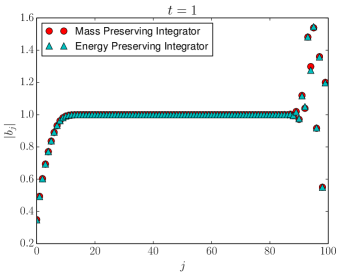
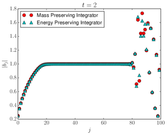
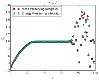
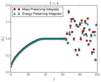
Figure 1. The integrators reproduce the rarefactive and dispersive wave-like behavior for initial condition (4.4) observed in [10, 18] and show agreement with one another. Computed with $\Delta{t}=0.1$.

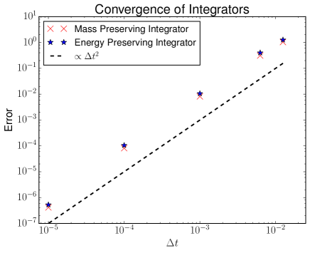
Figure 2. The error of integrators (2.5) and (2.6) compared to a high quality RK4 solution computed with $\Delta t=10^{-4}$, (4.5).

Table 1. Error, (4.5), computed using the surrogate RK4 solution.

$\Delta t$	Mass	Energy	Trapezoidal	Implicit Midpoint	Projection
0.1	0.18	0.20	0.19	0.20	0.11
0.05	0.06	0.07	0.07	0.07	0.02
0.025	0.02	0.02	0.02	0.02	2.32$\cdot 10^{-3}$
0.0125	5.05$\cdot 10^{-3}$	5.85$\cdot 10^{-3}$	5.56$\cdot 10^{-3}$	5.56$\cdot 10^{-3}$	3.06$\cdot 10^{-4}$

Table 2. Relative error in the mass invariant, $\max_{n}|\mathcal{M}[\mathbf{b}_{n}]-\mathcal{M}|/\mathcal{M}$.

$\Delta t$	Mass	Energy	Trapezoidal	Implicit Midpoint	Projection
0.1	2.84$\cdot 10^{-16}$	1.59$\cdot 10^{-4}$	3.82$\cdot 10^{-4}$	7.11$\cdot 10^{-16}$	1.99$\cdot 10^{-15}$
0.05	4.26$\cdot 10^{-16}$	3.87$\cdot 10^{-5}$	1.53$\cdot 10^{-4}$	2.84$\cdot 10^{-16}$	2.13$\cdot 10^{-15}$
0.025	7.11$\cdot 10^{-16}$	9.60$\cdot 10^{-6}$	4.69$\cdot 10^{-5}$	5.68$\cdot 10^{-16}$	3.41$\cdot 10^{-15}$
0.0125	5.68$\cdot 10^{-16}$	2.39$\cdot 10^{-6}$	1.26$\cdot 10^{-5}$	4.26$\cdot 10^{-16}$	6.54$\cdot 10^{-15}$

Table 3. Relative error in the energy invariant, $\max_{n}|\mathcal{H}[\mathbf{b}_{n}]-\mathcal{H}|/\mathcal{H}$.

$\Delta t$	Mass	Energy	Trapezoidal	Implicit Midpoint	Projection
0.1	9.33$\cdot 10^{-4}$	1.85$\cdot 10^{-15}$	4.43$\cdot 10^{-3}$	2.51$\cdot 10^{-3}$	5.54$\cdot 10^{-15}$
0.05	4.87$\cdot 10^{-4}$	1.71$\cdot 10^{-15}$	2.07$\cdot 10^{-3}$	1.09$\cdot 10^{-3}$	3.68$\cdot 10^{-14}$
0.025	1.75$\cdot 10^{-4}$	1.85$\cdot 10^{-15}$	6.96$\cdot 10^{-4}$	3.53$\cdot 10^{-4}$	1.14$\cdot 10^{-15}$
0.0125	5.00$\cdot 10^{-5}$	1.85$\cdot 10^{-15}$	1.95$\cdot 10^{-4}$	9.77$\cdot 10^{-5}$	2.88$\cdot 10^{-14}$

4.2. Performance of Nonlinear Solvers

As our proposed methods require solving a nonlinear system at each time step, the number of required Newton iterations bears consideration. Here, we repeat the numerical experiment of Section 4.1, solving (4.4) with $N=100$, and integrate out to $t_{\max}=1$. The results, with the same tolerances, are given in Tables 4 and 5. The Mass, Energy, Trapezoidal Rule, and Implicit Midpoint solvers had comparable performance, with no discernible advantages. Between four and six function evaluations are needed for these solvers per time step for each of these. In contrast, the Projection method typically took fewer function evaluations, but requires the additional four function evaluations from RK4. Thus, as measured by the number of function evaluations, these solvers, and RK4, are quite comparable.

A modest number of between three and five iterations of the Newton solver are needed for the implicit solvers, while the projection method typically requiring only two to three. The Projection method has the significant advantage of requiring a much smaller system to be solved. For all of solvers, analytic Jacobians were provided which offered a significant reduction in the number of function evaluations.

Table 4. Average number of function evaluations needed per time step.

$\Delta t$	Mass	Energy	Trapezoidal	Implicit Midpoint	Projection
0.1	5.00	5.00	5.00	5.00	4.00
0.05	4.62	5.00	5.70	5.70	3.35
0.025	5.00	5.00	5.00	5.00	3.00
0.0125	5.00	5.00	5.00	5.00	3.00

Table 5. Average number of Newton iterations needed per time step.

$\Delta t$	Mass	Energy	Trapezoidal	Implicit Midpoint	Projection
0.1	4.00	4.00	4.00	4.00	3.00
0.05	3.62	4.00	4.70	4.70	2.35
0.025	4.00	4.00	4.00	4.00	2.00
0.0125	4.00	4.00	4.00	4.00	2.00

4.3. Ensemble Simulations and Weak Turbulence

One way to measure energy transfer in (1.2) is through the Sobolev type $h^{s}$ norm

(4.6) $$\|\mathbf{b}(t)\|_{h^{s}}^{2}=\sum_{j=1}^{N}2^{(s-1)j}|b_{j}(t)|^{2}.$$

This is closely related to the measurements for energy transfer in [9, 10]. For a single initial condition, we may find that $h^{s}$ norm grows in time, but for a phenomenon to constitute weak turbulence, we would expect such a transfer to be generic. Thus, we simulate an ensemble of initial conditions and examine the average evolution of (4.6).

Our ensemble of initial conditions are constructed as follows. For the $k$-th sample,

(4.7) $$b_{j}^{(k)}(0)=\frac{1}{4^{j-1}}\cdot\exp\{i\theta_{j}^{(k)}\},\quad j=1,\ldots,N,$$

where $\theta_{j}^{(k)}\sim U(0,2\pi)$ are independently and identically distributed. The purpose of the decay in (4.7) is such that when we look at the large $N$ limit, the $h^{s}$ norms remain finite for $s\leq 4$. Our random phases were generated in parallel using the Scalable Parallel Random Number Generator (SPRNG) 2.0, [20], available at http://www.sprng.org. Our sample size in each case was one hundred.

The results of several of our simulations are shown Figures 3 and 4 where we plot the ensemble averaged evolution of the $h^{s}$ norm,

(4.8) $$\left\langle\left\|\mathbf{b}(t)\right\|_{h^{s}}\right\rangle=\frac{1}{M}\sum_{k=1}^{M}\left\|\mathbf{b}^{(k)}(t)\right\|_{h^{s}}$$

for different integrators using different time steps. First, in all cases, there is a generic tendency for the norms to grow. Second, as shown in Figure 3, the conservative schemes show consistent growth rates, independent of time step, out to $t_{\max}=1000$. One notable feature is that modified midpoint mass preserving integrator, (2.5), appears to have a comparatively larger variance than the other symmetric methods.

In Figure 4, we compare the conservative integrators to each other, along with Trapezoidal Rule and RK4. Again, there is consistency in the the ensemble averaged behavior. While we have only plotted the results for $s=4$, this is consistent with the other norms we have examined.

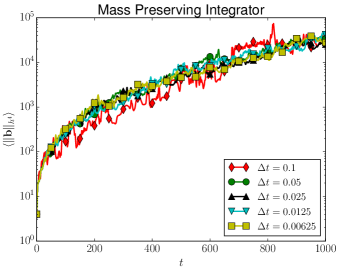
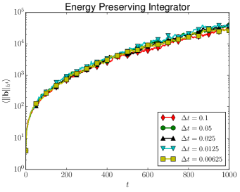
Figure 3. Ensemble averaged norm evolution for two conservative integrators and different values of $\Delta{t}$. In all cases, the ensemble averages were consistent as a function of time.

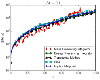
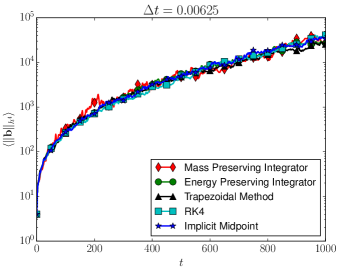
Figure 4. Ensemble averaged norm evolution for several integrators. On this time scale, the four methods are consistent at both values of $\Delta{t}$.

On longer time scales, we see the advantage of our conservative integrators. Integrating out to $t_{\max}=10^{5}$, we see a systematic bias in the norm, shown in Figure 5. To better understand this, we examine the ensemble averaged energy and mass invariants for the four methods. These are shown in Figure 6. Our conservative integrators and trapezoidal rule behave well, while the errors in mass and energy continue to grow when the RK4 method is used. Thus, on long time scales, fixed step Runge-Kutta methods will give biased results.

The boundedness of the error in the energy of the symmetric schemes which do not conserve energy, is unsurprising. In particular, implicit midpoint, being symplectic, will conserve some modified Hamiltonian, $\tilde{H}$, which will be nearly preserved over very long periods of integration and converge to $H$ as $\Delta{t}\to 0$, [16].

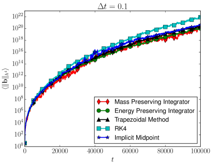
Figure 5. Ensemble averaged norm evolution of several of the integrators. On longer time scales, a large systematic bias appears in the RK4 Solution.

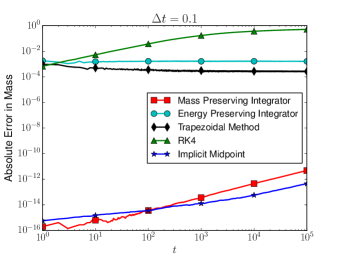
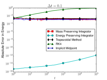
Figure 6. The conservative integrators accurately preserve the appropriate invariants of the system. Trapezoidal Rule is more consistent than RK4, which systematically adds energy to the system.

5. Discussion

We have formulated integrators which conserve the invariants of the Toy Model System, (1.2). The local truncation error in both cases is second order, and they provide robust behavior in simulations. However, we were only able to prove convergence of schemes which conserve mass, as we needed an a priori bound on the solution. One outstanding question is thus to prove convergence of the energy preserving scheme. Another is to produce a method that intrinsically preserves both invariants, without projection.

In comparison to other methods, these schemes are quite favorable, both in terms of their properties and computational cost. For large scale, long time, statistical studies, they will inevitably perform better than fixed step Runge-Kutta methods, though adaptive RK methods may outperform them.

References

- Balay et al. [1997] S. Balay, W. D. Gropp, L. C. McInnes, and B. F. Smith. Efficient management of parallelism in object oriented numerical software libraries. In E. Arge, A. M. Bruaset, and H. P. Langtangen, editors, Modern Software Tools in Scientific Computing, pages 163–202. Birkhäuser Press, 1997.
- Balay et al. [2016a] S. Balay, S. Abhyankar, M. F. Adams, J. Brown, P. Brune, K. Buschelman, L. Dalcin, V. Eijkhout, W. D. Gropp, D. Kaushik, M. G. Knepley, L. C. McInnes, K. Rupp, B. F. Smith, S. Zampini, H. Zhang, and H. Zhang. PETSc users manual. Technical Report ANL-95/11 - Revision 3.7, Argonne National Laboratory, 2016a. URL http://www.mcs.anl.gov/petsc.
- Balay et al. [2016b] S. Balay, S. Abhyankar, M. F. Adams, J. Brown, P. Brune, K. Buschelman, L. Dalcin, V. Eijkhout, W. D. Gropp, D. Kaushik, M. G. Knepley, L. C. McInnes, K. Rupp, B. F. Smith, S. Zampini, H. Zhang, and H. Zhang. PETSc Web page. http://www.mcs.anl.gov/petsc, 2016b. URL http://www.mcs.anl.gov/petsc.
- Bourgain [2004] J. Bourgain. Remarks on stability and diffusion in high-dimensional Hamiltonian systems and partial differential equations. Ergodic Theory and Dynamical Systems, 24(5):1331–1357, 2004.
- Cai and McLaughlin [2000] D. Cai and D. W. McLaughlin. Chaotic and turbulent behavior of unstable one-dimensional nonlinear dispersive waves. Journal Of Mathematical Physics, 41(6):4125–4153, May 2000.
- Cai et al. [1999] D. Cai, A. Majda, and D. W. McLaughlin. Spectral bifurcations in dispersive wave turbulence. Proceedings of the …, 96(24):14216–14221, 1999.
- Cai et al. [2001] D. Cai, A. J. Majda, D. W. McLaughlin, and E. G. Tabak. Dispersive wave turbulence in one dimension. Physica D: Nonlinear Phenomena, 152-153:551–572, Apr. 2001.
- Celledoni et al. [2012] E. Celledoni, V. Grimm, R. I. McLachlan, D. I. McLaren, D. O’Neale, B. Owren, and G. R. W. Quispel. Preserving energy resp. dissipation in numerical PDEs using the ”Average Vector Field” method. Journal Of Computational Physics, 231(20):6770–6789, Aug. 2012.
- Colliander et al. [2010] J. Colliander, M. Keel, G. Staffilani, H. Takaoka, and T. Tao. Transfer of energy to high frequencies in the cubic defocusing nonlinear Schrödinger equation. Inventiones Mathematicae, 181(1):39–113, 2010.
- Colliander et al. [2013] J. E. Colliander, J. L. Marzuola, T. Oh, and G. Simpson. Behavior of a Model Dynamical System with Applications to Weak Turbulence. Experimental Mathematics, 22(3):250–264, Sept. 2013.
- Cooper [1987] G. J. Cooper. Stability of Runge-Kutta methods for trajectory problems. IMA Journal of Numerical Analysis, 7(1):1–13, 1987.
- Delfour et al. [1981] M. Delfour, M. Fortin, and G. Payr. Finite-difference solutions of a non-linear Schroedinger equation. Journal Of Computational Physics, 44(2):277–288, Nov. 1981.
- Dyachenko et al. [1992] S. Dyachenko, A. C. Newell, A. Pushkarev, and V. E. Zakharov. Optical turbulence: weak turbulence, condensates and collapsing filaments in the nonlinear Schrödinger equation. Physica D: Nonlinear Phenomena, 57(1-2):96–160, May 1992.
- Faou [2012] E. Faou. Geometric numerical integration and Schrödinger equations. Zurich Lectures in Advanced Mathematics. European Mathematical Society (EMS), Zürich, Zuerich, Switzerland, 2012.
- Faou et al. [2016] E. Faou, P. Germain, and Z. Hani. The weakly nonlinear large-box limit of the 2D cubic nonlinear Schrödinger equation. Journal of the American Mathematical Society, 29(4):915–982, Oct. 2016.
- Hairer et al. [2006] E. Hairer, C. Lubich, and G. Wanner. Geometric Numerical Integration. Structure-Preserving Algorithms for Ordinary Differential Equations. Springer Science & Business Media, May 2006.
- Hani [2013] Z. Hani. Long-time Instability and Unbounded Sobolev Orbits for Some Periodic Nonlinear Schrödinger Equations. Archive for Rational Mechanics and Analysis, 211(3):929–964, Nov. 2013.
- Herr and Marzuola [2013] S. Herr and J. L. Marzuola. On discrete rarefaction waves in a nonlinear Schrödinger equation toy model for weak turbulence. arXiv preprint arXiv:1307.1873, 2013.
- Majda et al. [1997] A. J. Majda, D. W. McLaughlin, and E. G. Tabak. A one-dimensional model for dispersive wave turbulence. Journal of Nonlinear Science, 7(1):9–44, 1997.
- Mascagni and Srinivasan [2000] M. Mascagni and A. Srinivasan. Algorithm 806: Sprng: A scalable library for pseudorandom number generation. ACM Transactions on Mathematical Software (TOMS), 26(3):436–461, 2000.
- Matsuo and Furihata [2001] T. Matsuo and D. Furihata. Dissipative or Conservative Finite-Difference Schemes for Complex-Valued Nonlinear Partial Differential Equations. Journal Of Computational Physics, 171(2):425–447, July 2001.
- Rudin [1976] W. Rudin. Principles of Mathematical Analysis. McGraw-Hill, 1976.
- Tao [2016] M. Tao. Explicit symplectic approximation of nonseparable Hamiltonians: Algorithm and long time performance. Physical Review E, 94(4):043303, 2016.
- Zakharov et al. [2001] V. Zakharov, P. Guyenne, A. Pushkarev, and F. Dias. Wave turbulence in one-dimensional models. Physica D: Nonlinear Phenomena, 152-153:573–619, 2001.