On Mixed Memberships and Symmetric Nonnegative Matrix Factorizations

Abstract

The problem of finding overlapping communities in networks has gained much attention recently. Optimization-based approaches use non-negative matrix factorization (NMF) or variants, but the global optimum cannot be provably attained in general. Model-based approaches, such as the popular mixed-membership stochastic blockmodel or MMSB [1], use parameters for each node to specify the overlapping communities, but standard inference techniques cannot guarantee consistency. We link the two approaches, by (a) establishing sufficient conditions for the symmetric NMF optimization to have a unique solution under MMSB, and (b) proposing a computationally efficient algorithm called GeoNMF that is provably optimal and hence consistent for a broad parameter regime. We demonstrate its accuracy on both simulated and real-world datasets.

1 Introduction

Community detection is a fundamental problem in network analysis. It has been widely used in a diverse set of applications ranging from link prediction in social networks [26], predicting protein-protein or protein-DNA interactions in biological networks [8], to network protocol design such as data forwarding in delay tolerant networks [17].

Traditional community detection assumes that every node in the network belongs to exactly one community, but many practical settings call for greater flexibility. For instance, individuals in a social network may have multiple interests, and hence are best described as members of multiple interest-based communities. We focus on the popular mixed membership stochastic blockmodel (MMSB) [1] where each node $i$, $i\in[n]$ has a discrete probability distribution ${\bm{\theta}}_{i}=\left(\theta_{i1},\ldots,\theta_{iK}\right)$ over $K$ communities. The probability of linkage between nodes $i$ and $j$ depends on the degree of overlap between their communities:

$${\bm{\theta}}_{i} \sim\mathrm{Dirichlet}({\bm{\alpha}}) i\in[n]$$

$${\bf P} =\rho{\bm{\Theta}}{\bf B}{\bm{\Theta}}^{T}$$

$${\bf A}_{ij}={\bf A}_{ji} =\mathrm{Bernoulli}({\bf P}_{ij}) i,j\in[n]$$

where ${\bm{\theta}}_{i}$ is the $i$-th row of ${\bm{\Theta}}$, ${\bf A}$ represents the adjacency matrix of the generated graph, and ${\bf B}\in\mathbb{R}^{K\times K}$ is the community-community interaction matrix. The parameter $\rho$ controls the sparsity of the graph, so WLOG, the largest entry of ${\bf B}$ can be set to 1. The parameter $\alpha_{0}=\sum_{i}\alpha_{i}$ controls the amount of overlap. In particular, when $\alpha_{0}\rightarrow 0$, MMSB reduces to the well known stochastic blockmodel, where every node belongs to exactly one community. Larger $\alpha_{0}$ leads to more overlap. Since we only observe ${\bf A}$, a natural question is: how can $\{{\bm{\theta}}_{i}\}$ and ${\bf B}$ be recovered from ${\bf A}$ in a way that is provably consistent?

1.1 Prior work

We categorize existing approaches broadly into three groups: model-based parameter inference methods, specialized algorithms that offer provable guarantees, and optimization-based methods using non-negative matrix factorization.

Model-based methods: These apply standard techniques for inference of hidden variables to the MMSB model. Examples include MCMC techniques [5] and variational methods [10]. While these often work well in practice, there are no proofs of consistency for these methods. The MCMC methods are difficult to scale to large graphs, so we compare against the faster variational inference methods in our experiments.

Algorithms with provable guarantees: There has been work on provably consistent estimation on models similar to MMSB. Zhang et al. [31] propose a spectral method (OCCAM) for a model where the ${\bm{\theta}}_{i}$ has unit $\ell_{2}$ norm (unlike MMSB, where they have unit $\ell_{1}$ norm). In addition to the standard assumptions regarding the existence of “pure” nodes (which only belong to a single community) and a positive-definite ${\bf B}$, they also require ${\bf B}$ to have equal diagonal entries, and assume that the ground truth communities has a unique optimum of a special loss function, and there is curvature around the optimum. Such assumptions may be hard to verify. Ray et al. [24] and Kaufmann et al. [13] consider models with binary community memberships. Kaufmann et al. [13] show that the global optimum of a special loss function is consistent. However, achieving the global optimum is computationally intractable, and the scalable algorithm proposed by them (SAAC) is not provably consistent. Anandkumar et al. [2] propose a tensor based approach for MMSB. Despite their elegant solution the computational complexity is $O(n^{2}K)$, which can be prohibitive for large graphs.

Optimization-based methods: If ${\bf B}$ is positive-definite, the MMSB probability matrix ${\bf P}$ can be written as ${\bf P}={\bf W}{\bf W}^{T}$, where the ${\bf W}$ matrix has only non-negative entries. In other words, ${\bf W}$ is the solution to a Symmetric Non-negative Matrix Factorization (SNMF) problem: ${\bf W}=\arg\min_{{\bf X}\geq{\bf 0}}\text{loss}({\bf P},{\bf X}{\bf X}^{T})$ for some loss function that measure the “difference” between ${\bf P}$ and its factorization. SNMF has been widely studied and successfully used for community detection [14, 28, 29, 23], but typically lacks the guarantees we desire. Our paper attempts to address these issues.

We note that Arora et al. [3, 4] used NMF to consistently estimate parameters of a topic model. However, their results cannot be easily applied to the MMSB inference problem. In particular, for topic models, the columns of the word-by-topic matrix specifying the probability distribution of words in a topic sum to 1. For MMSB, the rows of the node membership matrix sum to 1. The relationship of this work to the MMSB problem is unclear.

1.2 Problem Statement and Contributions

We seek to answer two problems.

Problem 1: Given ${\bf P}$, when does the solution to the SNMF optimization yield the correct ${\bf W}$?

The difficulty stems from the fact that (a) the MMSB model may not always be identifiable, and (b) even if it is, the corresponding SNMF problem may not have a unique solution (even after allowing for permutation of communities).

Even when the conditions for Problem 1 are met, we may be unable to find a good solution in practice. This is due to two reasons. First, we only know the adjacency matrix ${\bf A}$, and not the probability matrix ${\bf P}$. Second, the general SNMF problem is non-convex, and SNMF algorithms can get stuck at local optima. Hence, it is unclear if an algorithm can consistently recover the MMSB parameters. This leads to our next question.

Problem 2: Given ${\bf A}$ generated from a MMSB model, can we develop a fast and provably consistent algorithm to infer the parameters?

Our goal is to develop a fast algorithm that provably solves SNMF for an identifiable MMSB model. Note that generic SNMF algorithms typically do not have any provable guarantees.

Our contributions are as follows.

Identifiability: We show conditions that are sufficient for MMSB to be identifiable; specifically, there must be at least one “pure” exemplar of each of the $K$ clusters (i.e., a node that belongs to that community with probability $1$), and ${\bf B}$ must be full rank.

Uniqueness under SNMF: We provide sufficient conditions under which an identifiable MMSB model is the unique solution for the SNMF problem; specifically, the MMSB probability matrix ${\bf P}$ has a unique SNMF solution if ${\bf B}$ is diagonal. It is important to note that MMSB with a diagonal ${\bf B}$ still allows for interactions between different communities via members who belong to both.

Recovery algorithm: We present a new algorithm, called GeoNMF, for recovering the parameters $\{{\bm{\theta}}_{i}\}$ and ${\bf B}$ given only the observed adjacency matrix ${\bf A}$. The only compute-intensive part of the algorithm is the calculation of the top-$K$ eigenvalues and eigenvectors of ${\bf A}$, for which highly optimized algorithms exist [22].

Provable guarantees: Under the common assumption that ${\bm{\theta}}_{i}$ are generated from a Dirichlet(${\bm{\alpha}}$) prior, we prove the consistency of GeoNMF when ${\bf B}$ is diagonal and there are “pure” nodes for each cluster (exactly the conditions needed for uniqueness of SNMF). We allow the sparsity parameter $\rho$ to decay with the graph size $n$. All proofs are deferred to the appendix.

Empirical validation: On simulated networks, we compare GeoNMF against variational methods (SVI) [10]. Since OCCAM, SAAC, and BSNMF (a Bayesian variant of SNMF [23]) are formed under different model assumptions, we exclude these for the simulation experiments for fairness. We also run experiments on Facebook and Google Plus ego networks collected by Mcauley and Leskovec [18]; co-authorship datasets constructed by us from DBLP [16] and the Microsoft academic graph (MAG) [25]. These networks can have up to 150,000 nodes. On these graphs we compare GeoNMF against SVI, SAAC, OCCAM and BSNMF. We see that GeoNMF is consistently among the top, while also being one of the fastest. This establishes that GeoNMF achieves excellent accuracy and is computationally efficient in addition to being provably consistent.

2 Identifiability and Uniqueness

In order to present our results, we will now introduce some key definitions. Similar definitions appear in [31].

Definition 2.1.

A node $i\in[n]$ is called a “pure” node if $\exists$ $j\in[K]$ such that $\theta_{ij}=1$ and $\theta_{i\ell}=0$ for all $\ell\in[K]$, $\ell\neq j$.

Identifiability of MMSB. MMSB is not identifiable in general. Consider the following counter example.

$${\bf M}_{1} =\begin{bmatrix}0.5&0.5&0\\ 0&0.5&0.5\\ 0.5&0&0.5\end{bmatrix} {\bf M}_{2} =\begin{bmatrix}0.5&0.25&0.25\\ 0.25&0.5&0.25\\ 0.25&0.25&0.5\end{bmatrix}$$

It can be easily checked that the probability matrices ${\bf P}$ generated by the parameter set $({\bm{\Theta}}^{(1)},{\bf B}^{(1)},\rho^{(1)})=({\bf M}_{1},{\bf I}_{3\times 3},1)$ is exactly the same as that generated by $({\bm{\Theta}}^{(2)},{\bf B}^{(2)},\rho^{(2)})=({\bf I}_{3\times 3},2{\bf M}_{2},0.5)$, where ${\bf I}_{3\times 3}$ is the identity matrix. This example can be extended to arbitrarily large $n$: for every new row ${\bm{\theta}}_{i}^{(2)}$ added to ${\bm{\Theta}}^{(2)}$, add the row ${\bm{\theta}}_{i}^{(1)}={\bm{\theta}}_{i}^{(2)}{\bf M}_{1}$ to ${\bm{\Theta}}^{(1)}$. The new rows are still non-negative and sum to $1$; it can be verified that ${\bf P}^{(1)}={\bf P}^{(2)}$ even after these new node additions.

Thus, while MMSB is not identifiable in general, we can prove identifiability under certain conditions.

Theorem 2.1 (Sufficient conditions for MMSB identifiability).

Suppose parameters ${\bm{\Theta}},{\bf B}$ of the MMSB model satisfy the following conditions: (a) there is at least one pure node for each community, and (b) ${\bf B}$ has full rank. Then, MMSB is identifiable up to a permutation.

Since identifiability is a necessary condition for consistent recovery of parameters, we will assume these conditions from now on.

Uniqueness of SNMF for MMSB model. Even when the MMSB model is identifiable, the SNMF optimization may not have a unique solution. In other words, given an MMSB probability matrix ${\bf P}$, there might be multiple matrices ${\bf X}$ such that ${\bf P}={\bf X}{\bf X}^{T}$, even if ${\bf P}$ corresponds to a unique parameter setting $({\bm{\Theta}},{\bf B},\rho)$ under MMSB. For SNMF to work, ${\bf W}=\sqrt{\rho}{\bm{\Theta}}{\bf B}^{1/2}$ must the the unique SNMF solution. When does this happen?

In general, SNMF is not unique because ${\bf W}$ can be permuted, so we consider the following definition of uniqueness.

Definition 2.2.

(Uniqueness of SNMF [11]) The Symmetric NMF of ${\bf P}={\bf W}{\bf W}^{T}$ is said to be (essentially) unique if ${\bf P}=\tilde{{\bf W}}\tilde{{\bf W}}^{T}$ implies $\tilde{{\bf W}}={\bf W}{\bf Z}$, where ${\bf Z}$ is a permutation matrix.

Theorem 2.2 (Uniqueness of SNMF for MMSB).

Consider an identifiable MMSB model where ${\bf B}$ is diagonal. Then, its Symmetric NMF ${\bf W}$ is unique and equals $\sqrt{\rho}{\bm{\Theta}}{\bf B}^{1/2}$ .

The above results establish that if we find a ${\bf W}$ that is the symmetric NMF solution of ${\bf P}$ then it is at least unique. However, two practical questions are still unanswered. First, given the non-convex nature of SNMF, how can we guarantee that we find the correct ${\bf W}$ given ${\bf P}$? Second, in practice we are given not ${\bf P}$ but the noisy adjacency matrix ${\bf A}$. Typical algorithms for SNMF do not provide guarantees even for the first question.

3 Provably consistent inference for MMSB

To achieve consistent inference, we turn to the specific structure of the MMSB model. We motivate our approach in three stages. First, note that under the conditions of Theorem 2.2, the rows of ${\bf W}$ form a simplex whose corners are formed by the pure nodes for each cluster. In addition, these corners are aligned along different axes, and hence are orthogonal to each other. Thus, if we can detect the corners of the simplex, we can recover the MMSB parameters. So the goal is to find the pure nodes from different clusters, since they define the corners.

While our goal is to get ${\bf W}$, note that it is easy to compute ${\bf V}{\bf E}^{1/2}$ where ${\bf V},{\bf E}$ are the eigenvectors and eigenvalues of ${\bf P}$, i.e., ${\bf P}={\bf V}{\bf E}{\bf V}^{T}$. Thus, ${\bf W}{\bf W}^{T}=({\bf V}{\bf E}^{1/2})({\bf V}{\bf E}^{1/2})^{T}$. This implies that ${\bf W}={\bf V}{\bf E}^{1/2}{\bf Q}$ for some orthogonal matrix ${\bf Q}$ (Lemma A.1 of [27]). Essentially we should be able to identify the pure nodes by finding the corners of the simplex based on ${\bf V}$ and ${\bf E}$.

Once we have found the pure nodes, it is easy to find the rotation matrix ${\bf Q}$ modulo a permutaion of classes, because we know that the pure nodes are on the axis for the simplex of ${\bm{\Theta}}{\bf B}^{1/2}$.

Now, we note something rather striking. Let $\mathbfcal{D}$ denote the diagonal matrix with expected degrees on the diagonal. Consider the population Laplacian $\mathbfcal{D}^{-1/2}{\bf P}\mathbfcal{D}^{-1/2}$. Its square root is given by $\mathbfcal{D}^{-1/2}{\bf V}{\bf E}^{1/2}$, which has the following interesting property for equal Dirichlet parameters $\alpha_{a}=\alpha_{0}/K$. We show in Lemma 4.1 that while the resulting rows no longer fall on a simplex, the rows with the largest norm are precisely the pure nodes, for whom the norm concentrates around $\sqrt{K/n}$. Thus, picking the rows with the largest norm of the square root gives us the pure nodes. From this, ${\bf Q}$, ${\bm{\theta}}_{i}$ for other rows and the parameters $\rho$ and ${\bf B}$ can again be easily extracted.

Needless to say, this only answers the question for the expectation matrix ${\bf P}$. In reality, we have a noisy adjacency matrix. Let $\hat{{\bf V}}$ and $\hat{{\bf E}}$ denote the matrices of eigenvectors and eigenvalues of ${\bf A}$. We also establish in this paper that the rows of $\hat{{\bf V}}\hat{{\bf E}}^{1/2}$ concentrate around its population counterpart (corresponding row of ${\bf V}{\bf E}^{1/2}\bm{O}$ for some rotation matrix $\bm{O}$). While there are eigenvector deviation results in random matrix theory, e.g. the Davis-Kahan Theorem [9], these typically provide deviation results for the whole $\hat{{\bf V}}$ matrix, not its rows. In a nutshell, this crucial result lets us carefully bound the errors of each step of the same basic idea executed on ${\bf A}$, the noisy proxy for ${\bf P}$.

Algorithm 1 GeoNMF

0:  Adjacency matrix ${\bf A}$; number of communities $K$; a constant $\epsilon_{0}$

0:  Estimated node-community distribution matrix $\hat{{\bm{\Theta}}}$, Community-community interaction matrix $\hat{{\bf B}}$, sparsity-control parameter $\hat{\rho}$;

1:  Randomly split the set of nodes $[n]$ into two equal-sized parts $\mathcal{S}$ and $\bar{\mathcal{S}}$.

2:  Obtain the top $K$ eigen-decomposition of ${\bf A}(\mathcal{S},\mathcal{S})$ as $\hat{{\bf V}}_{1}\hat{{\bf E}}_{1}\hat{{\bf V}}_{1}^{T}$ and of ${\bf A}(\bar{\mathcal{S}},\bar{\mathcal{S}})$ as $\hat{{\bf V}}_{2}\hat{{\bf E}}_{2}\hat{{\bf V}}_{2}^{T}$.

3:  Calculate degree matrices ${\bf D}_{2}$, ${\bf D}_{12}$ and ${\bf D}_{21}$ for the rows of ${\bf A}(\bar{\mathcal{S}},\bar{\mathcal{S}})$, ${\bf A}(\mathcal{S},\bar{\mathcal{S}})$ and ${\bf A}(\bar{\mathcal{S}},\mathcal{S})$ respectively.

4:  $\hat{{\bf X}}={\bf D}_{21}^{-1/2}{\bf A}_{21}\hat{{\bf V}}_{1}\hat{{\bf E}}_{1}^{-1/2}$, where ${\bf A}_{21}={\bf A}(\bar{\mathcal{S}},\mathcal{S}).$

5:  $\mathcal{F}=\left\{i:\|\hat{{\bf X}}(i,:)\|_{2}\geq\left(1-\epsilon_{0}\right)\max_{j}\|\hat{{\bf X}}(j,:)\|_{2}\right\}$

6:  $\mathcal{S}_{p}=\text{PartitionPureNodes}$$\left(\hat{{\bf X}}(\mathcal{F},:),\sqrt{\frac{K}{4n}\frac{\min_{i\in\mathcal{F}}{\bf D}_{2}(i,i)}{\max_{i\in\mathcal{F}}{\bf D}_{2}(i,i)}}\right)$

7:  $\hat{{\bf X}}_{p}=\hat{{\bf X}}(\mathcal{S}_{p},:)$

8:  Get $\hat{{\bm{\beta}}}$, where $\hat{\beta}_{i}=\left\|{\bf e}_{i}^{T}{\bf D}_{21}^{1/2}(\mathcal{S}_{p},\mathcal{S}_{p})\hat{{\bf X}}_{p}\right\|_{2}^{2}$, $i\in[K]$

9:  $\hat{{\bf B}}=\mathrm{diag}(\hat{{\bm{\beta}}})$

10:  $\hat{\rho}=\max_{i}\hat{{\bf B}}_{ii}$

11:  $\hat{{\bf B}}=\hat{{\bf B}}/\hat{\rho}$

12:  $\hat{{\bm{\Theta}}}(\bar{\mathcal{S}},:)={\bf D}_{21}^{1/2}\hat{{\bf X}}\hat{{\bf X}}_{p}^{-1}{\bf D}_{21}^{-1/2}(\mathcal{S}_{p},\mathcal{S}_{p})$

13:  Repeat steps with ${\bf D}_{12}$, ${\bf A}_{12}$, $\hat{{\bf V}}_{2}$, and $\hat{{\bf E}}_{2}$ to obtain parameter estimates for the remaining bipartition.

Algorithm 1 shows our NMF algorithm based on these geometric intuitions for inference under MMSB (henceforth, GeoNMF). The complexity of GeoNMF is dominated by the one-time eigen-decomposition in step $2$. Thus this algorithm is fast and scalable. The consistency of parameters inferred under GeoNMF is shown in the next section.

Algorithm 2 PartitionPureNodes

0:  Matrix ${\bf M}\in\mathbb{R}^{m\times K}$, where each row represents a pure node; a constant $\tau$

0:  A set $S$ consisting of one pure node from each cluster.

1:  $S=\{\}$, $C=\{\}$.

2:  while  $C\neq[m]$  do

3:     Randomly pick one index from $[m]\setminus C$, say $s$

4:     $S=S\cup\{s\}$

5:     $C=C\cup\{i\in[m]\setminus C:\|{\bf M}(s,:)-{\bf M}(i,:)\|\leq\tau\}$

6:  end while

Remark 3.1.

Note that Algorithm 1 produces two sets of parameters for the two partitions of the graph $\mathcal{S}$ and $\bar{\mathcal{S}}$. In practice one may need to have parameter estimates of the entire graph. While there are many ways of doing this, the most intuitive way would be to look at the set of pure nodes in $\mathcal{S}$ (call this $\mathcal{S}_{p}$) and those in $\bar{\mathcal{S}}$ (call this $\bar{\mathcal{S}}_{p}$). If one looks at the subgraph induced by the union of all these pure nodes, then with high probability, there should be $K$ connected components, which will allow us to match the communities.

Also note that Algorithm 2 may return $k\neq K$ clusters. However, we show in Lemma 4.4 that the pure nodes extracted by our algorithm will be highly separated and with high probability we will have $k=K$ for an appropriately chosen $\tau$.

Finally, we note that, in our implementation, we construct the candidate pure node set $\mathcal{F}$ (step 5 of Algorithm 1) by finding all nodes with norm within $\epsilon_{0}$ multiplicative error of the largest norm. We increase $\epsilon_{0}$ from a small value, until $\hat{{\bf X}}_{p}$ has condition number close to one. This is helpful when $n$ is small, where asymptotic results do not hold.

4 Analysis

We want to prove that the sample-based estimates $\hat{{\bm{\Theta}}}$, $\hat{{\bf B}}$ and $\hat{\rho}$ concentrate around the corresponding population parameters ${\bm{\Theta}}$, ${\bf B}$, and $\rho$ after appropriate normalization. We will show this in several steps, which follow the steps of GeoNMF.

For the following statements, denote $\beta_{\mathrm{min}}=\min_{a}{\bf B}_{aa}$, ${\bm{\Theta}}_{2}={\bm{\Theta}}(\bar{\mathcal{S}},:)$, where $\bar{\mathcal{S}}$ is one of the random bipartitions of $[n]$. Let ${\mathbfcal{D}}_{21}$ be the population version of ${\bf D}_{21}$ defined in Algorithm 1. Also let $\hat{{\bf X}}_{i}={\bf e}_{i}^{T}{\bf D}_{21}^{-1/2}{\bf A}_{21}\hat{{\bf V}}_{1}\hat{{\bf E}}_{1}^{-1/2}$ and its population version ${\bf X}_{i}=\sqrt{\rho}\cdot{\bf e}_{i}^{T}{\mathbfcal{D}}_{21}^{-1/2}{\bm{\Theta}}_{2}{\bf B}^{1/2}$ for $i\in[\frac{n}{2}]$.

First we show the pure nodes have the largest row norm of the population version of $\hat{{\bf X}}$.

Lemma 4.1.

Recall that ${\bf X}\in\mathbb{R}^{\frac{n}{2}\times K}$. If ${\bm{\Theta}}\sim\text{Dirichlet}({\bm{\alpha}})$ with $\alpha_{i}=\alpha_{0}/K$, then $\forall i\in[\frac{n}{2}]$,

$$\left\|{\bf X}_{i}\right\|_{2}^{2}\leq\frac{2K}{n}\max_{a}\theta_{ia}{\left(1+O_{P}\left({\sqrt{\frac{K\log n}{n}}}\right)\right)}$$

with probability larger than $1-O(1/n^{3})$.

In particular, if node $i$ of subgraph ${\bf A}(\bar{\mathcal{S}},\bar{\mathcal{S}})$ is a pure node ($\max_{a}\theta_{ia}=1$),

$$\left\|{\bf X}_{i}\right\|_{2}^{2}\in\frac{2K}{n}{\left[1-O_{P}\left({\sqrt{\frac{K\log n}{n}}}\right),1+O_{P}\left({\sqrt{\frac{K\log n}{n}}}\right)\right]}.$$

Concentration of rows of $\hat{{\bf X}}$. We must show that the rows of the sample $\hat{{\bf X}}$ matrix concentrate around a suitably rotated population version. While it is known that $\hat{{\bf V}}$ concentrates around suitably rotated ${\bf V}$ (see the variant of Davis-Kahan Theorem presented in [30]), these results are for columns of the ${\bf V}$ matrix, not for each row. The trivial bound for row-wise error would be to upper bound it by the total error, which is too crude for our purposes. To get row-wise convergence, we use sample-splitting (similar ideas can be found in [19, 7]), as detailed in steps 1 to 4 of GeoNMF. The key idea is to split the graph in two parts and project the adjacency matrix of one part onto eigenvectors of another part. Due to independence of these two parts, one can show concentration.

Theorem 4.2.

Consider an adjacency matrix ${\bf A}$ generated from MMSB$({\bm{\Theta}},{\bf B},\rho$), where ${\bm{\Theta}}\sim\text{Dirichlet}({\bm{\alpha}})$ with $\alpha_{i}=\alpha_{0}/K$, whose parameters satisfy the conditions of Theorem 2.2. If $\rho n=\Omega(\log n)$, then $\exists$ orthogonal matrix $\bm{O}\in\mathbb{R}^{K\times K}$ that $\forall\ i\in[\frac{n}{2}]$,

$$\frac{\|\hat{{\bf X}}_{i}-{\bf X}_{i}\bm{O}\|_{2}}{\left\|{\bf X}_{i}\right\|_{2}}=O_{P}\left({\frac{{K^{2}\sqrt{\log n}}}{\beta_{\mathrm{min}}^{5/2}\rho\sqrt{n}}}\right)$$

with probability larger than $1-O(K^{2}/n^{2})$.

Thus, the sample-based quantity for each row $i$ converges to its population variant.

Selection of pure nodes. GeoNMF selects the nodes with (almost) the highest norm. We prove that this only selects nearly pure nodes. Let $\epsilon^{\prime}=O_{P}\left({\frac{{K^{2}\sqrt{\log n}}}{\beta_{\mathrm{min}}^{5/2}\rho\sqrt{n}}}\right)$ represent the row-wise error term from Theorem 4.2.

Lemma 4.3.

Let $\mathcal{F}$ be the set of nodes with $\|\hat{{\bf X}}_{i}\|_{2}\geq(1-\epsilon_{0})\max_{j}\|\hat{{\bf X}}_{j}\|_{2}$. Then $\forall i\in\mathcal{F}$,

$$\max_{a}\theta_{ia}\geq 1-O_{P}(\epsilon_{0}+\epsilon^{\prime})$$

with probability larger than $1-O(K^{2}/n^{2})$.

We choose $\epsilon_{0}=O_{P}(\epsilon^{\prime})$ and it is straightforward to show by Lemmas 4.1, 4.3, and Theorem 4.2 that if $\epsilon_{0}\geq 2\epsilon^{\prime}$, then $\mathcal{F}$ includes all pure nodes from all $K$ communities.

Clustering of pure nodes. Once the (nearly) pure nodes have been selected, we run PartitionPureNodes (Algorithm 2) on them. We show that these nodes can form exactly $K$ well separated clusters and each cluster only contains nodes whose ${\bm{\theta}}$ are peaked on the same element, and PartitionPureNodes can select exactly one node from each of the $K$ communities.

Lemma 4.4.

Let $\tau=\sqrt{\frac{K}{4n}\frac{\min_{i\in\mathcal{F}}{\bf D}_{2}(i,i)}{\max_{i\in\mathcal{F}}{\bf D}_{2}(i,i)}}$, where $\mathcal{F}$ is defined in step 5 of Algorithm 1. If all conditions in Theorem 4.2 are satisfied, then PartitionPureNodes ($\hat{{\bf X}}(\mathcal{F},:),\tau$) returns one (nearly) pure node from each of the underlying $K$ communities with probability larger than $1-O(K^{2}/n^{2})$.

Concentration of $(\hat{{\bm{\Theta}}},\hat{{\bf B}},\hat{\rho})$. GeoNMF recovers ${\bm{\Theta}}$ using ${\bf D}$, $\hat{{\bf X}}$, and its pure portion $\hat{{\bf X}}_{p}$ (via the inverse $\hat{{\bf X}}_{p}^{-1}$). We first prove that $\hat{{\bf X}}_{p}^{-1}$ concentrates around its expectation.

Theorem 4.5.

Let $\mathcal{S}_{p}$ be the set of of pure nodes extracted using our algorithm. Let $\hat{{\bf X}}_{p}$ denote the rows of $\hat{{\bf X}}$ indexed by $\mathcal{S}_{p}$. Then, for the orthogonal matrix $\bm{O}$ from Theorem 4.2,

$$\frac{\|\hat{{\bf X}}_{p}^{-1}-\left({\bf X}_{p}\bm{O}\right)^{-1}\|_{F}}{\|{\bf X}_{p}^{-1}\|_{F}}=O_{P}\left({\frac{{K^{5/2}\sqrt{\log n}}}{\beta_{\mathrm{min}}^{5/2}\rho\sqrt{n}}}\right)$$

with probability larger than $1-O(K^{2}/n^{2})$.

Next, we shall prove consistency for $\hat{{\bm{\Theta}}}_{2}:=\hat{{\bm{\Theta}}}(\bar{\mathcal{S}},:)$; the proof for $\hat{{\bm{\Theta}}}(\mathcal{S},:)$ is similar. Let ${\bf D}_{21p}={\bf D}_{21}(\mathcal{S}_{p},\mathcal{S}_{p})$.

Theorem 4.6.

Let $\hat{{\bm{\Theta}}}_{2}={\bf D}_{21}^{1/2}\hat{{\bf X}}\hat{{\bf X}}_{p}^{-1}{\bf D}_{21p}^{-1/2}$, then $\exists$ a permutation matrix ${\bf\Pi}\in\mathbb{R}^{K\times K}$ such that

$$\frac{\|\hat{{\bm{\Theta}}}_{2}-{\bm{\Theta}}_{2}{\bf\Pi}\|_{F}}{\|{\bm{\Theta}}_{2}\|_{F}}=O_{P}\left({\frac{K^{3}\sqrt{\log n}}{\beta_{\mathrm{min}}^{3}\rho\sqrt{n}}}\right)$$

with probability larger than $1-O(K^{2}/n^{2})$.

Recall that ${\bf B}$ and $\hat{{\bf B}}$ are both diagonal matrices, with diagonal components $\{\beta_{a}\}$ and $\{\hat{\beta}_{a}\}$ respectively.

Theorem 4.7.

Let $\hat{\rho}\hat{\beta}_{a}=\|{\bf e}_{a}^{T}{\bf D}_{21}^{1/2}(\mathcal{S}_{p},\mathcal{S}_{p})\hat{{\bf X}}_{p}\|_{2}^{2}$. Then, $\exists$ a permutation matrix ${\bf\Pi}\in\mathbb{R}^{K\times K}$ such that $\forall a\in[K]$,

$$\hat{\rho}\hat{\beta}_{a}\in\rho\beta_{a^{\prime}}\left[1-O_{P}\left(\frac{{K^{5/2}\log n}}{\beta_{\mathrm{min}}^{5/2}\rho\sqrt{n}}\right),1+O_{P}\left(\frac{{K^{5/2}\log n}}{\beta_{\mathrm{min}}^{5/2}\rho\sqrt{n}}\right)\right]$$

for some $a^{\prime}$ such that ${\bf\Pi}_{a^{\prime}a}=1$, with probability larger than $1-O(K^{2}/n^{2})$.

Remark 4.1.

While the details of our algorithms were designed for obtaining rigorous theoretical guarantees, many of these can be relaxed in practice. For instance, while we require the Dirichlet parameters to be equal, leading to balanced cluster sizes, real data experiments show that our algorithm works well for unbalanced settings as well. Similarly, the algorithm assumes a diagonal ${\bf B}$ (which is sufficient for uniqueness), but empirically works well even in the presence of off-diagonal noise. Finally, splitting the nodes into $\mathcal{S}$ and $\bar{\mathcal{S}}$ is not needed in practice.

5 Experiments

We present results on simulated and real-world datasets. Via simulations, we evaluate the sensitivity of GeoNMF to the various MMSB parameters: the skewness of the diagonal elements of ${\bf B}$ and off-diagonal noise, the Dirichlet parameter ${\bm{\alpha}}$ that controls the degree of overlap, the sparsity parameter $\rho$, and the number of communities $K$. Then, we evaluate GeoNMF on Facebook and Google Plus ego networks, and co-authorship networks with upto 150,000 nodes constructed from DBLP and the Microsoft Academic Network.

Baseline methods: For the real-world networks, we compare GeoNMF against the following methods:

• Stochastic variational inference (SVI) for MMSB [10],

• a Bayesian variant of SNMF for overlapping community detection (BSNMF) [23],

• the OCCAM algorithm [31] for recovering mixed memberships, and

• the SAAC algorithm [13].

For the simulation experiments, we only compare GeoNMF against SVI, since these are the only two methods based specifically on the MMSB model. BSNMF has a completely different underlying model, OCCAM requires rows of ${\bm{\Theta}}$ to have unit $\ell_{2}$ norm and ${\bf B}$ to have equal diagonal elements, and SAAC requires ${\bm{\Theta}}$ to be a binary matrix, while MMSB requires rows of ${\bm{\Theta}}$ to have unit $\ell_{1}$ norm.

Since the community identities can only be recovered up-to a permutation, in both simulated and real data experiments, we figure out the order of the communities using the well known Munkres algorithm in [21].

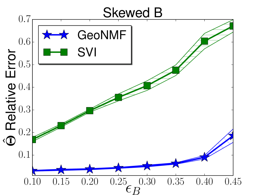
(a)

$\rho=1,{\bf B}=\text{diag}({\bm{\beta}}/\max_{i}\beta_{i})$,

${\bm{\beta}}=(0.5-\epsilon_{B},0.5,0.5+\epsilon_{B})$

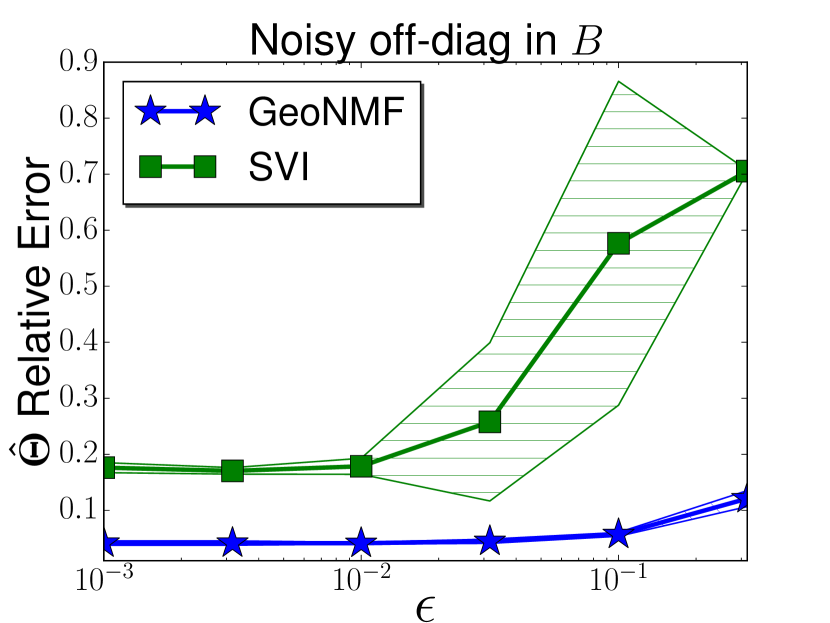
(b)

${\bf B}=\text{diag}({\bm{\beta}}-\epsilon\cdot{\bf 1}_{K})+\epsilon\cdot{\bf 1}_{K}{\bf 1}_{K}^{T}$,

${\bm{\beta}}=(0.6,0.8,1),\rho=1$

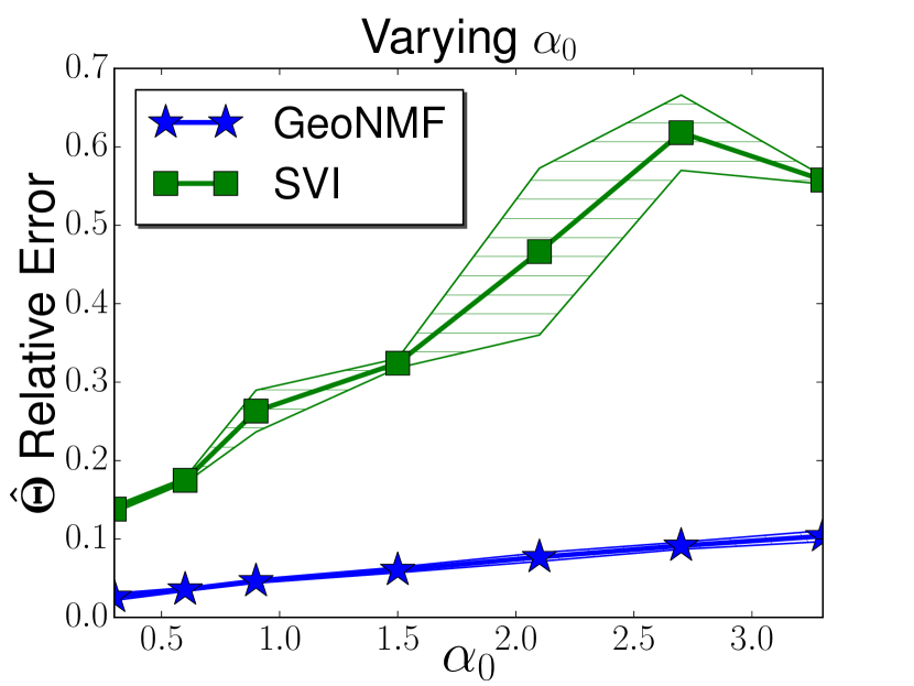
(c)

$\rho=0.7,{\bf B}=\text{diag}({\bm{\beta}}$),

${\bm{\beta}}=(0.4,0.7,1)$

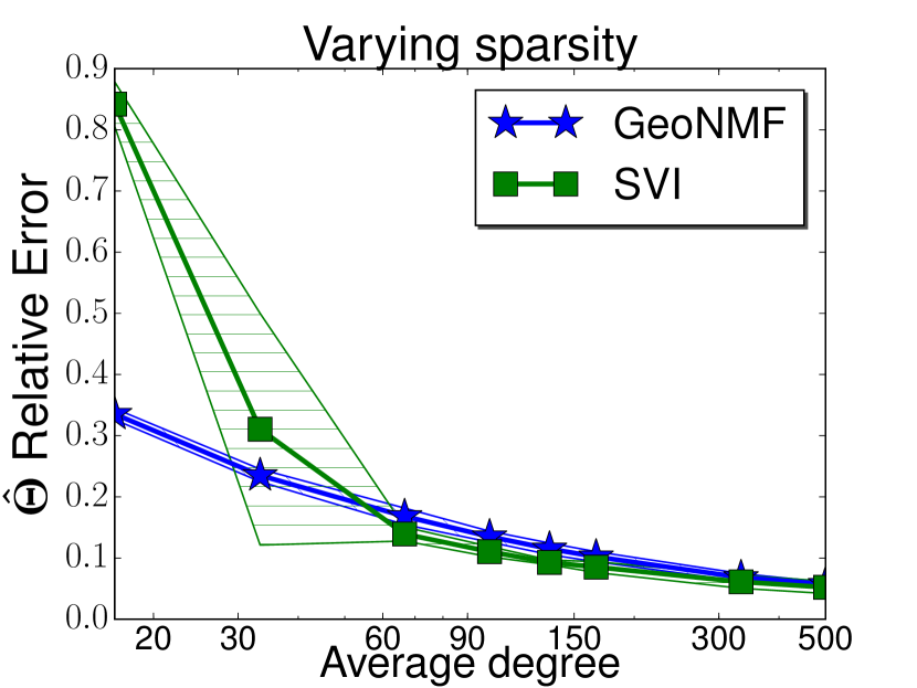
(d)

${\bf B}=\text{diag}({\bm{\beta}})$,

${\bm{\beta}}=(1,1,1),\rho=1$

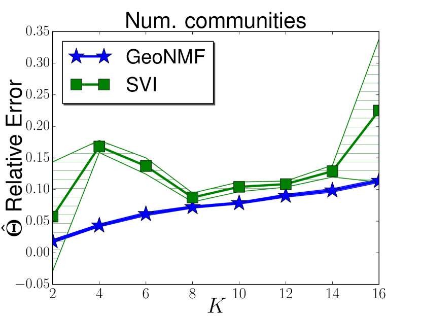
(e)

${\bf B}=\text{diag}(0.35\cdot{\bf 1}_{K}+0.65\cdot{\bf r}_{K})$,

${\bf r}_{K}=\text{rand}(K,1),\rho=1$

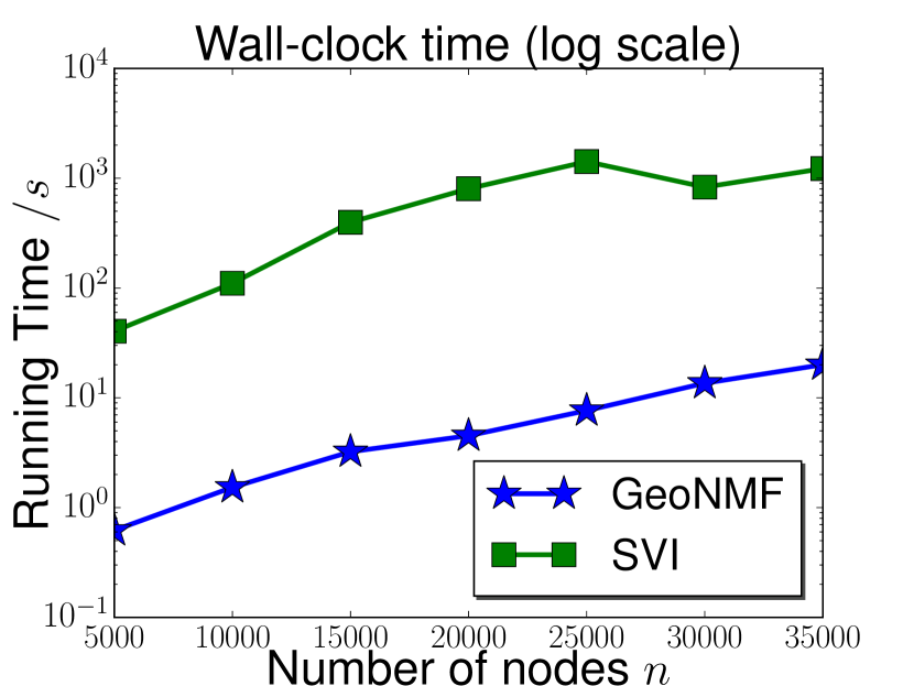
(f)

${\bf B}=\text{diag}(0.5\cdot{\bf 1}_{K}+0.5\cdot{\bf r}_{K})$,

${\bf r}_{K}=\text{rand}(K,1),\rho=1$

Figure 1: 1(a)-1(e) Simulation results for varying parameters. 1(f) Running time.

5.1 Simulated data

Our simulations with the MMSB model are shown in Figure 1. We use $\alpha_{i}=\alpha_{0}/K$ for $i\in[K]$. While this leads to balanced clusters, note that the real datasets have clusters of different sizes and we will show that GeoNMF works consistently well even for those networks (see Section 5.2). Unless otherwise stated, we set $n=5000$, $K=3$, and $\alpha_{0}=1$.

Evaluation Metric: Since we have ground truth ${\bm{\Theta}}$, we report the relative error of the inferred MMSB parameters ${\bm{\Theta}}$ defined as $\min\limits_{{\bf\Pi}}\frac{\left\|\hat{{\bm{\Theta}}}-{\bm{\Theta}}{\bf\Pi}\right\|_{F}}{\left\|{\bm{\Theta}}\right\|_{F}}$. Here the minimum is taken over all $K\times K$ permutation matrices. For each experiment, we report the average and the standard deviation over $10$ random samples. Since all the baseline algorithms only return $\hat{{\bm{\Theta}}}$, we only report relative error of that.

Sensitivity to skewness of the diagonal of ${\bf B}$: Let ${\bm{\beta}}=\text{diag}({\bf B})$. For skewed ${\bm{\beta}}$, different communities have different strengths of connection. We use ${\bm{\beta}}=(0.5-\epsilon_{B},0.5,0.5+\epsilon_{B})$ and plot the relative error against varying $\epsilon_{B}$. Figure  1(a) shows that GeoNMF has much smaller error than SVI, and is robust to ${\bm{\beta}}$ over a wide range.

Sensitivity to off-diagonal element ${\bf B}$: While SNMF is identifiable only for diagonal ${\bf B}$, we still test GeoNMF in the setting where all off-diagonal entries of ${\bf B}$ have noise $\epsilon$. Figure 1(b) shows once again that GeoNMF is robust to such noise, and is much more accurate than SVI.

Sensitivity to $\alpha_{0}$: In Figure  1(c), the relative error is plotted against increasing $\alpha_{0}$; larger values corresponding to larger overlap between communities. Accuracy degrades with increasing overlap, as expected, but GeoNMF is much less affected than SVI.

Sensitivity to $\rho$: Figure 1(d) shows relative error against increasing $\rho$. For dense networks, both GeoNMF and SVI perform similarly, but the error of SVI increases drastically in the sparse regime (small $\rho$).

Scalability: Figure 1(f) shows the wall-clock time for networks of different sizes. Both GeoNMF and SVI scale linearly with the number of nodes, but SVI is about 100 times slower than GeoNMF.

5.2 Real-world data

Datasets: For real-data experiments, we use two kinds of networks:

• Ego networks: We use the Facebook and Google Plus (G-plus) ego networks, where each node can be part of multiple “circles” or “communities.”

• Co-authorship networks: We construct co-authorship networks from DBLP (each community is a group of conferences), and from the Microsoft Academic Graph (each community is denoted by a “field of study” (FOS) tag). Each author’s ${\bm{\theta}}$ vector is constructed by normalizing the number of papers he/she has published in conferences in a subfield (or papers that have the FOS tag).

Table 1: Network statistics

Dataset	Facebook	G-plus	DBLP1	DBLP2	DBLP3	DBLP4	DBLP5	MAG1	MAG2
$\#$ nodes $n$	362.0 ($\pm$ 148.5)	656.2 ($\pm$ 422.0)	30,566	16,817	13,315	25,481	42,351	142,788	108,064
$\#$ communities $K$	2.3 ($\pm$0.58)	2.8 ($\pm$1.74)	6	3	3	3	4	3	3
Average Degree	56.8 ($\pm$32.3)	103.4 ($\pm$74.9)	8.9	7.6	8.5	5.2	6.8	12.4	16.0
Overlap $\%$	19.3($\pm$29.8)	26.5 ($\pm$32.4)	18.2	14.9	21.1	14.4	18.5	3.3	3.8

We preprocessed the networks by recursively removing isolated nodes, communities without any pure nodes, and nodes with no community assignments. For the ego networks we pick networks with at least 200 nodes and the average number of nodes per community ($n/K$) is at least 100, giving us 3 Facebook and and 40 G-plus networks. For the co-authorship networks, all communities have enough pure nodes, and after removing isolated nodes, the networks have more than 200 nodes and $n/K$ is larger than 100. The statistics of the networks (number of nodes, average degree, number of clusters, degree of overlap etc.) are shown in Table 1. The overlap ratio is the number of overlapping nodes divided by the number of nodes. The different networks have the following subfields:

• DBLP1: Machine Learning, Theoretical Computer Science, Data Mining, Computer Vision, Artificial Intelligence, Natural Language Processing

• DBLP2: Networking and Communications, Systems, Information Theory

• DBLP3: Databases, Data Mining, World Web Wide

• DBLP4: Programming Languages, Software Engineering, Formal Methods

• DBLP5: Computer Architecture, Computer Hardware, Real-time and Embedded Systems, Computer-aided Design

• MAG1: Computational Biology and Bioinformatics, Organic Chemistry, Genetics

• MAG2: Machine Learning, Artificial Intelligence, Mathematical Optimization

Evaluation Metric: For real data experiments, we construct ${\bm{\Theta}}$ as follows. For the ego-networks every node has a binary vector which indicates which circle (community) each node belongs to. We normalize this to construct ${\bm{\Theta}}$. For the DBLP and Microsoft Academic networks we construct a row of ${\bm{\Theta}}$ by normalizing the number of papers an author has in different conferences (ground truth communities). We present the averaged Spearman rank correlation coefficients (RC) between ${\bm{\Theta}}(:,a)$, $a\in[K]$ and $\hat{{\bm{\Theta}}}(:,\sigma(a))$, where $\sigma$ is a permutation of $[K]$. The formal definition is:

$$\mathrm{RC}_{\mathrm{avg}}(\hat{{\bm{\Theta}}},{\bm{\Theta}}) =\frac{1}{K}\max_{\sigma}\sum_{i=1}^{K}\text{RC}(\hat{{\bm{\Theta}}}(:,i),{\bm{\Theta}}(:,\sigma(i))).$$

It is easy to see that $\mathrm{RC}_{\mathrm{avg}}(\hat{{\bm{\Theta}}},{\bm{\Theta}})$ takes value from -1 to 1, and higher is better. Since SAAC returns binary assignment, we compute its $\text{RC}_{\text{avg}}$ against the binary ground truth.

(a)

(b)

(c)

(d)

(e)

(f)

Figure 2: $\text{RC}_{\text{avg}}$ and running time (log scale) for real datasets.

Performance: We report the $\mathrm{RC}_{\mathrm{avg}}$ score in Figure 2(a) averaged over different Faceboook and G-plus networks; in Figure 2(b) for five DBLP networks, and in Figure 2(c) for two MAG networks. We show the time in seconds (log-scale) in Figure 2(d) averaged over Facebook and G-plus networks; in Figure 2(e) for DBLP networks and in Figure 2(f) for MAG networks. We averaged over the Facebook and G-plus networks because all the performances were similar.

• For small networks like Facebook and G-plus, all algorithms perform equally well both in speed and accuracy, although GeoNMF is fast even for relatively larger G-plus networks.

• DBLP is sparser, and as a result the overall rank correlation decreases. However, GeoNMF consistently performs well . While for some networks, BSNMF and OCCAM have comparable $\mathrm{RC}_{\mathrm{avg}}$, they are much slower than GeoNMF.

• MAG is larger (hundreds of thousands of nodes) than DBLP. For these networks we could not even run BSNMF because of memory issues. Again, GeoNMF performs consistently well while outperforming others in speed.

Estimating $K$: While we assume that $K$ is known apriori, $K$ can be estimated using the USVT estimator [6]. For the simulated graphs, when average degree is above ten, USVT estimates $K$ correctly. However for the real graphs, which are often sparse, it typically overestimates the true number of clusters.

6 Conclusions

This paper explored the applicability of symmetric NMF algorithms for inference of MMSB parameters. We showed broad conditions that ensure identifiability of MMSB, and then proved sufficiency conditions for the MMSB parameters to be uniquely determined by a general symmetric NMF algorithm. Since general-purpose symmetric NMF algorithms do not have optimality guarantees, we propose a new algorithm, called GeoNMF, that adapts symmetric NMF specifically to MMSB. GeoNMF is not only provably consistent, but also shows good accuracy in simulated and real-world experiments, while also being among the fastest approaches.

Appendix

Appendix A Identifiability

Lemma A.1.

(Lemma 1.1 of [20]) The inverse of a nonnegative matrix matrix ${\bf M}$ is nonnegative if and only if ${\bf M}$ is a generalized permutation matrix.

Proof of Theorem 2.1.

Suppose there are two parameter settings $({\bm{\Theta}}^{(1)}$, ${\bf B}^{(1)}$, $\rho^{(1)})$ and $({\bm{\Theta}}^{(2)}$, ${\bf B}^{(2)}$, $\rho^{(2)})$ that yield the same probability matrix:

$${\bf P}=\rho^{(1)}{\bm{\Theta}}^{(1)}{\bf B}^{(1)}{{\bm{\Theta}}^{(1)}}^{T}=\rho^{(2)}{\bm{\Theta}}^{(2)}{\bf B}^{(2)}{{\bm{\Theta}}^{(2)}}^{T}.$$

Pick up pure node indices set $\mathcal{I}_{1}$ of ${\bm{\Theta}}^{(1)}$ such that ${\bm{\Theta}}_{\mathcal{I}_{1}}^{(1)}={\bf I}$, and denote ${\bf M}={\bm{\Theta}}_{\mathcal{I}_{1}}^{(2)}$. Similarly, pick up pure node indices set $\mathcal{I}_{2}$ of ${\bm{\Theta}}^{(2)}$ such that ${\bm{\Theta}}_{\mathcal{I}_{2}}^{(2)}={\bf I}$, and let ${\bf W}={\bm{\Theta}}_{\mathcal{I}_{2}}^{(1)}$.

Then

$$\rho^{(1)}{\bf B}^{(1)}=\rho^{(2)}{\bf M}{\bf B}^{(2)}{\bf M}^{T}\ \text{ and }\ \rho^{(1)}{\bf W}{\bf B}^{(1)}{\bf W}^{T}=\rho^{(2)}{\bf B}^{(2)}.$$

Denote ${\bf T}={\bf M}{\bf W}$, then

$${\bf B}^{(1)}=\frac{1}{\rho^{(1)}}{\bf M}\rho^{(1)}{\bf W}{\bf B}^{(1)}{\bf W}^{T}{\bf M}^{T}={\bf T}{\bf B}^{(1)}{\bf T}^{T}.$$ (1)

Note that ${\bf M}\cdot{\bf 1}={\bm{\Theta}}_{\mathcal{I}_{1}}^{(2)}\cdot{\bf 1}={\bf 1}$ and ${\bf W}\cdot{\bf 1}={\bm{\Theta}}_{\mathcal{I}_{2}}^{(1)}\cdot{\bf 1}={\bf 1}$, so ${\bf T}\cdot{\bf 1}={\bf M}{\bf W}\cdot{\bf 1}={\bf 1}$. We can consider ${\bf T}$ as a transition matrix of a Markov chain, whose states are the nodes of the graph. Keep applying equation (1) to its RHS, we get

$${\bf B}^{(1)}={\bf T}^{k}{\bf B}^{(1)}{{\bf T}^{k}}^{T},$$

which implies ${\bf B}^{(1)}={\bf T}_{\infty}{\bf B}^{(1)}{\bf T}_{\infty}^{T}$, where ${\bf T}_{\infty}=\lim\limits_{k\rightarrow\infty}{\bf T}^{k}$.

Given that ${\bf B}^{(1)}$ has full rank $K$, we must have ${\bf T}_{\infty}$ has full rank. Now we prove that stationary point of the Markov chain, ${\bf T}_{\infty}$, must be identity matrix.

The nodes of a finite-size Markov chain can be split into a finite number of communication classes, and possibly some transient nodes.

1. If a communication class has at least two nodes and is aperiodic, then the rows corresponding to those nodes in ${\bf T}_{\infty}$ are the stationary distribution for that class. Hence, ${\bf T}_{\infty}$ has identical rows, so it cannot be full rank.

2. The probability of a Markov chain ending in a transient node goes to zero as the number of iterations $k$ grows, so the column of ${\bf T}_{\infty}$ corresponding to any transient node is identically zero. Again, this means that ${\bf T}_{\infty}$ cannot be full rank.

Hence, the only configuration in which ${\bf T}_{\infty}$ has full rank is when it contains $K$ communication classes, each with one node. This implies that ${\bf T}_{\infty}={\bf I}$, and hence ${\bf T}={\bf I}$. Note that if the communication classes are periodic, we can consider ${\bf T}^{t}$ where $t$ is the product of the periods of all the classes; the matrix ${\bf T}^{t}$ is now aperiodic for all the communication classes, and the above argument still applies to ${\bf T}_{\infty}=\lim\limits_{k\rightarrow\infty}({{\bf T}^{t}})^{k}$.

As ${\bf I}={\bf T}={\bf M}{\bf W}$, ${\bf M}$ and ${\bf W}$ have full rank, then ${\bf M}^{-1}={\bf W}$, which is the case that a nonnegative matrix ${\bf M}$ has nonnegative inverse ${\bf W}$, using Lemma A.1, we know that ${\bf M}$ is a generalized permutation matrix, and note that each row of ${\bf M}$ sums to 1, the scale goes away and thus ${\bf M}$ is a permutation matrix, which implies ${\bf W}$ is also a permutation matrix. As largest element of ${{\bf B}^{(1)}}$ and ${{\bf B}^{(2)}}$ are equals as 1, we should have $\rho^{(1)}=\rho^{(2)}$ and thus ${{\bf B}^{(1)}}={\bf M}{{\bf B}^{(2)}}{\bf M}^{T}$.

Also since we have

$$\rho^{(1)}{\bf B}^{(1)}{{\bm{\Theta}}^{(1)}}^{T} =\rho^{(1)}{\bm{\Theta}}_{\mathcal{I}_{1}}^{(1)}{\bf B}^{(1)}{{\bm{\Theta}}^{(1)}}^{T}=\rho^{(2)}{\bm{\Theta}}_{\mathcal{I}_{1}}^{(2)}{\bf B}^{(2)}{{\bm{\Theta}}^{(2)}}^{T}=\rho^{(2)}{\bf M}{\bf B}^{(2)}{{\bm{\Theta}}^{(2)}}^{T}$$

$$=\rho^{(2)}{\bf M}{\bf B}^{(2)}{\bf M}^{T}{\bf M}{{\bm{\Theta}}^{(2)}}^{T}=\rho^{(1)}{\bf B}^{(1)}{\bf M}{{\bm{\Theta}}^{(2)}}^{T},$$

left multiply $\left(\rho^{(1)}{\bf B}^{(1)}\right)^{-1}$ on both sides, we have ${{\bm{\Theta}}^{(1)}}={{\bm{\Theta}}^{(2)}}{\bf M}^{T}$.

Thus we have shown that MMSB is identifiable up to a permutation. ∎

Appendix B Uniqueness of SNMF for MMSB networks

Lemma B.1 (Huang et al. [11]).

If $\text{rank}({\bf P})=K$, the Symmetric NMF ${\bf P}={\bf W}{\bf W}^{T}$ is unique if and only if the non-negative orthant is the only self-dual simplicial cone $\mathcal{A}$ with $K$ extreme rays that satisfies $\mathrm{cone}({{\bf W}}^{T})\subseteq\mathcal{A}=\mathcal{A}^{*}$, where $\mathcal{A}^{*}$ is the dual cone of $\mathcal{A}$, defined as $\mathcal{A}^{*}=\{{\bf y}|{\bf x}^{T}{\bf y}\geq 0,\forall{\bf x}\in\mathcal{A}\}$.

Proof of Theorem 2.2.

When ${\bf B}$ is diagonal, it has a square root ${\bf C}={\bf B}^{1/2}$, where ${\bf C}$ is also a positive diagonal matrix. It is easy to see that $\mathrm{cone}({\bf C})$ is the non-negative orthant $\mathbb{R}_{+}^{K}$, so we have

$$\mathrm{cone}({\bf W}^{T})=\mathrm{cone}({\bf C}^{T}{\bm{\Theta}}^{T})=\mathrm{cone}({\bf C}^{T})=\mathrm{cone}({\bf C})=\mathbb{R}_{+}^{K}={\mathbb{R}_{+}^{K}}^{*}.$$

The second equality follows from the fact that ${\bm{\Theta}}$ contains all pure nodes, and other nodes are convex combinations of these pure nodes. The fourth equality is due to the diagonal form of ${\bf C}$.

To see that this is unique, suppose there is another self-dual simplicial cone satisfying $\mathrm{cone}({{\bf W}}^{T})\subseteq\mathcal{A}=\mathcal{A}^{*}$. Then we have $\mathbb{R}_{+}^{K}\subseteq\mathcal{A}$ and $\mathcal{A}=\mathcal{A}^{*}\subseteq{\left(\mathbb{R}_{+}^{K}\right)}^{*}=\mathbb{R}_{+}^{K}$, which implies $\mathcal{A}=\mathbb{R}_{+}^{K}$.

Hence, by Lemma B.1, an identifiable MMSB model with a diagonal ${\bf B}$ is sufficient for the Symmetric NMF solution to be unique and correct. ∎

Appendix C Concentration of the Laplacian

We will use $X=c(1\pm\epsilon)$ to denote $X\in c[1-\epsilon,1+\epsilon]$ for ease of notation from now onwards.

Lemma C.1.

For ${\bm{\Theta}}\in\mathbb{R}^{n\times K}$, where each row ${\bm{\theta}}_{i}\sim\mathrm{Dirichlet}({\bm{\alpha}})$, $\forall j\in[K]$,

$$\sum_{i=1}^{n}\theta_{ij}=n\frac{\alpha_{j}}{\alpha_{0}}\left(1\pm O_{P}\left(\sqrt{\frac{\alpha_{0}}{\alpha_{j}}\frac{\log n}{n}}\right)\right)$$

with probability larger than $1-1/n^{3}$.

Proof.

By using Chernoff bound

$$\mathrm{P}\left(\left|\sum_{i=1}^{n}\theta_{ij}-n\frac{\alpha_{j}}{\alpha_{0}}\right|>\epsilon n\frac{\alpha_{j}}{\alpha_{0}}\right)\leq\exp\left(-\frac{\epsilon^{2}n\frac{\alpha_{j}}{\alpha_{0}}}{3}\right),$$

so by setting $\epsilon=O_{P}\left(3\sqrt{\frac{{\log n}}{n{\alpha_{j}}/{\alpha_{0}}}}\right)$, ${\left|\sum_{i=1}^{n}\theta_{ij}-n\frac{\alpha_{j}}{\alpha_{0}}\right|\leq 3\sqrt{{\frac{\alpha_{j}}{\alpha_{0}}n\log n}},}$ with probability larger than $1-1/n^{3}$.

That is

$$\sum_{i=1}^{n}\theta_{ij} =n\frac{\alpha_{j}}{\alpha_{0}}\pm O_{P}\left(\sqrt{{\frac{\alpha_{j}}{\alpha_{0}}n\log n}}\right)=n\frac{\alpha_{j}}{\alpha_{0}}\left(1\pm O_{P}\left(\sqrt{\frac{\alpha_{0}}{\alpha_{j}}\frac{\log n}{n}}\right)\right).$$

∎

Lemma C.2.

(Theorem 5.2 of [15]) Let ${\bf A}$ be the adjacency matrix of a random graph on $n$ nodes in which edges occur independently. Set $\mathrm{E}[{\bf A}]={\bf P}$ and assume that $n\max_{i,j}{\bf P}_{ij}\leq d$ for $d\geq c_{0}\log n$ and $c_{0}>0$. Then, for any $r>0$ there exists a constant $C=C(r,c_{0})$ such that:

$$\mathrm{P}(\left\|{\bf A}-{\bf P}\right\|\leq C\sqrt{d})\geq 1-n^{-r}.$$

Fact C.1.

If ${\bf M}$ is rank $k$, then $\|{\bf M}\|_{F}^{2}\leq k\|{\bf M}\|^{2}$.

Lemma C.3.

(Variant of Davis-Kahan [30]). Let ${\bf P}$, $\hat{{\bf A}}\in\mathbb{R}^{n\times n}$ be symmetric, with eigenvalues $\lambda_{1}\geq\cdots\geq\lambda_{n}$ and $\hat{\lambda}_{1}\geq\cdots\geq\hat{\lambda}_{n}$ respectively. Fix $1\leq r\leq s\leq n$, and assume that $\min(\lambda_{r-1}-\lambda_{r},\lambda_{s}-\lambda_{s+1})>0$, where we define $\lambda_{0}=\infty$ and $\lambda_{n+1}=-\infty$. Let $d=s-r+1$, and let ${\bf V}=({\bf v}_{r},{\bf v}_{r+1},\cdots,{\bf v}_{s})\in\mathbb{R}^{n\times d}$ and $\hat{V}=(\hat{{\bf v}}_{r},\hat{{\bf v}}_{r+1},\cdots,\hat{{\bf v}}_{s})\in\mathbb{R}^{n\times d}$ have orthonormal columns satisfying ${\bf P}{\bf v}_{j}=\lambda_{j}{\bf v}_{j}$ and $\hat{{\bf A}}\hat{{\bf v}}_{j}=\hat{\lambda}_{j}\hat{{\bf v}}_{j}$ for $j=r,r+1,\cdots,s$. Then there exists an orthogonal matrix $\hat{{\bf O}}\in\mathbb{R}^{d\times d}$ such that

$$\left\|\hat{{\bf V}}-{\bf V}\hat{{\bf O}}\right\|_{F}\leq\frac{2^{3/2}\min\left(d^{1/2}\left\|\hat{{\bf A}}-{\bf P}\right\|,\left\|\hat{{\bf A}}-{\bf P}\right\|_{F}\right)}{\min(\lambda_{r-1}-\lambda_{r},\lambda_{s}-\lambda_{s+1})}$$

Lemma C.4.

(Lemma A.1. of [27]). Let ${\bf H}_{1}$, ${{\bf H}_{2}}\in\mathbb{R}^{n\times n}$ be positive semidefinite with $\mathrm{rank}({\bf H}_{1})=\mathrm{rank}({\bf H}_{2})=K$. Let ${\bf X},{\bf Y}\in\mathbb{R}^{n\times K}$ be of full column rank such that ${\bf X}{\bf X}^{T}={\bf H}_{1}$ and ${\bf Y}{\bf Y}^{T}={\bf H}_{2}$. Let $\lambda_{K}\left({\bf H}_{2}\right))$ be the smallest nonzero eigenvalue of ${\bf H}_{2}$. Then there exists an orthogonal matrix ${\bf R}\in\mathbb{R}^{K\times K}$ such that:

$$\left\|{{\bf X}{\bf R}}-{\bf Y}\right\|_{F}\leq\frac{\sqrt{K}\left\|{{\bf H}_{1}}-{\bf H}_{2}\right\|\left(\sqrt{\left\|{{\bf H}_{1}}\right\|}+\sqrt{\left\|{\bf H}_{2}\right\|}\right)}{\lambda_{K}\left({\bf H}_{2}\right)}.$$

Lemma C.5.

Recall that $\hat{{\bf A}}_{1}=\hat{{\bf V}}_{1}\hat{{\bf E}}_{1}\hat{{\bf V}}_{1}^{T}$ and ${\bf P}_{1}={\bf P}(\mathcal{S},\mathcal{S})$ in Algorithm 1. If $\rho n=\Omega(\log n)$, then

$$\left\|\hat{{\bf A}}_{1}-{\bf P}_{1}\right\|=O_{P}(\sqrt{\rho n}),\text{ and }\left\|\hat{{\bf A}}_{1}-{\bf P}_{1}\right\|_{F}=O_{P}(\sqrt{K\rho n})$$

with probability larger than $1-1/n^{3}$.

Proof.

Lemma C.2 gives the spectral bound of binary symmetric random matrices, in our model,

$$\frac{n}{2}\max_{i,j}{\bf P}_{1}(i,j)\leq\frac{n}{2}\max_{i,j}{\bf P}(i,j)=\frac{n}{2}\max_{i,j}\rho{\bm{\theta}}_{i}{\bf B}{\bm{\theta}}_{j}^{T}\leq\frac{n}{2}\max_{i,j}\rho{\bm{\theta}}_{i}{\bf I}{\bm{\theta}}_{j}^{T}\leq\rho\frac{n}{2}.$$

Note that we need to use ${\bf B}$ is diagonal probability matrix and ${\bm{\theta}}_{i}$, $i\in[\frac{n}{2}]$ has $\ell_{1}$ norm 1 and all nonnegative elements for the last two inequality.

Since $\rho n=\Omega(\log n)$, $\exists c_{0}\geq 0$ that $\rho\frac{n}{2}\geq c_{0}\log\frac{n}{2}$.

Let $d=\rho\frac{n}{2}$, then $d\geq\frac{n}{2}\max_{i,j}{\bf P}_{1}(i,j)$ and $d\geq c_{0}\log\frac{n}{2}$, by Lemma C.2, $\forall r\geq 0$, $\exists$ $C>0$ that

$$\mathrm{P}\left(\left\|{\bf A}_{1}-{\bf P}_{1}\right\|\leq C\sqrt{\rho\frac{n}{2}}\right)\geq 1-(\frac{n}{2})^{-r},$$

where ${\bf A}_{1}={\bf A}(\mathcal{S},\mathcal{S})$. So $\left\|{\bf A}_{1}-{\bf P}_{1}\right\|=O_{P}(\sqrt{\rho n})$, specially, taking $r=3$ then it is with probability larger than $1-1/n^{3}$. Hence

$$\left\|\hat{{\bf A}}_{1}-{\bf P}_{1}\right\|\leq\left\|\hat{{\bf A}}_{1}-{\bf A}_{1}+{\bf A}_{1}-{\bf P}_{1}\right\|\leq\left\|\hat{{\bf A}}_{1}-{\bf A}_{1}\right\|+\left\|{\bf A}_{1}-{\bf P}_{1}\right\|=\hat{\sigma}_{K+1}+O_{P}(\sqrt{\rho n})=O_{P}(\sqrt{\rho n}),$$

where $\hat{\sigma}_{K+1}$ is the $(K+1)$-th eigenvalue of ${\bf A}_{1}$ and is $O_{P}(\sqrt{\rho n})$ by Weyl’s inequality.

Since $\hat{{\bf A}}_{1}$ and ${\bf P}_{1}$ have rank $K$, then by Fact C.1,

$$\left\|\hat{{\bf A}}_{1}-{\bf P}_{1}\right\|_{F}\leq\sqrt{2K}\left\|\hat{{\bf A}}_{1}-{\bf P}_{1}\right\|=O_{P}(\sqrt{K\rho n}).$$

∎

Lemma C.6 (Concentration of degrees).

Denote $\beta_{\mathrm{min}}=\min_{a}{\bf B}_{aa}$. Let ${\bf P}=\rho{\bm{\Theta}}^{(1)}{\bf B}{{\bm{\Theta}}^{(2)}}^{T}$, where $\rho$, ${\bf B}$, ${\bm{\Theta}}^{(1)}\in\mathbb{R}^{\frac{n}{2}\times K}$, and ${\bm{\Theta}}^{(2)}\in\mathbb{R}^{\frac{n}{2}\times K}$ follow the restrictions of MMSB model. Let ${\bf D}$ and ${\mathbfcal{D}}$ be diagonal matrices representing the sample and population node degrees. Then

$${\mathbfcal{D}}_{ii}=O_{P}(\rho n/K),\ {\mathbfcal{D}}_{ii}=\Omega(\beta_{\mathrm{min}}\rho n/K),\ \text{ and }\ \ \left|{\bf D}_{ii}-{\mathbfcal{D}}_{ii}\right|=O_{P}(\sqrt{\rho n\log n/K})$$

with probability larger than $1-O_{P}(1/n^{3})$.

Proof.

$\forall i\in[\frac{n}{2}]$, we have

$${\mathbfcal{D}}_{ii} =\sum_{j=1}^{n/2}P_{ij}=\sum_{j=1}^{n/2}\sum_{\ell=1}^{K}\rho\theta_{i\ell}^{(1)}{\bf B}_{\ell\ell}{\theta}_{j\ell}^{(2)}\leq\sum_{\ell=1}^{K}\rho\theta_{i\ell}^{(1)}\sum_{j=1}^{n/2}{\theta}_{j\ell}^{(2)}=\rho\sum_{\ell=1}^{K}\theta_{i\ell}^{(1)}\sum_{j=1}^{n/2}{\theta}_{j\ell}^{(2)} \max_{a}{\bf B}_{aa}=1$$ ( by definition)

$$=\rho n\frac{\sum_{\ell=1}^{K}\theta_{i\ell}^{(1)}\alpha_{l}}{\alpha_{0}}\left(\frac{1}{2}+O_{P}\left(\sqrt{\frac{\alpha_{0}}{\alpha_{l}}\frac{\log n}{n}}\right)\right)$$ (from Lemma C.1)

$$=\frac{\rho n}{2K}\left(1+O_{P}\left(\sqrt{\frac{K\log n}{n}}\right)\right), \alpha_{k}=\frac{\alpha_{0}}{K},\forall k\in[K]$$ (when )

so ${\mathbfcal{D}}_{ii}=O_{P}(\rho n/K)$.

Similarly,

$${\mathbfcal{D}}_{ii} \geq\sum_{\ell=1}^{K}\beta_{\mathrm{min}}\rho\theta_{i\ell}^{(1)}\sum_{j=1}^{n/2}{\theta}_{j\ell}^{(2)}=\beta_{\mathrm{min}}\rho\sum_{\ell=1}^{K}\theta_{i\ell}^{(1)}\sum_{j=1}^{n/2}{\theta}_{j\ell}^{(2)}$$

$$=\beta_{\mathrm{min}}\rho n\frac{\sum_{\ell=1}^{K}\theta_{i\ell}^{(1)}\alpha_{l}}{\alpha_{0}}\left(\frac{1}{2}+O_{P}\left(\sqrt{\frac{\alpha_{0}}{\alpha_{l}}\frac{\log n}{n}}\right)\right)$$ (from Lemma C.1)

$$=\frac{\beta_{\mathrm{min}}}{2K}\rho n\left(1+O_{P}\left(\sqrt{\frac{K\log n}{n}}\right)\right), \alpha_{l}=\frac{\alpha_{0}}{K},\forall l$$ (when )

so ${\mathbfcal{D}}_{ii}=\Omega(\beta_{\mathrm{min}}\rho n/K)$.

Then using Chernoff bound, we have

$$\mathrm{P}\left(\left|{\bf D}_{ii}-{\mathbfcal{D}}_{ii}\right|>\epsilon{\mathbfcal{D}}_{ii}]\right)\leq\exp\left(-\frac{\epsilon^{2}{\mathbfcal{D}}_{ii}}{3}\right),$$

so when $\epsilon=O_{P}\left(3\sqrt{\frac{{K\log n}}{\rho n}}\right)$, $\left|{\bf D}_{ii}-{\mathbfcal{D}}_{ii}\right|\leq\epsilon{\mathbfcal{D}}_{ii}=O_{P}(\sqrt{\rho n\log n/K})$ with probability at least $1-1/n^{3}$. Note we have used Lemma C.1, so in total it is with probability larger than $1-O_{P}(1/n^{3})$.

∎

Lemma C.7.

Denote $\beta_{\mathrm{min}}=\min_{a}{\bf B}_{aa}$. If $\rho n=\Omega(\log n)$, then

$$\lambda_{K}({\bf P}_{1})=\Omega(\beta_{\mathrm{min}}\rho n/K),\quad\lambda_{1}({\bf P}_{1})=O_{P}\left(\rho n/K\right)$$

and

$$\lambda_{K}({\bf A}_{1})=\Omega(\beta_{\mathrm{min}}\rho n/K),\quad\lambda_{1}({\bf A}_{1})=O_{P}\left(\rho n/K\right)$$

with probability larger than $1-O_{P}(K^{2}/n^{3})$.

Proof.

For conciseness, we will omit the subscript $1$ (see Lemma C.5) in the following proof without loss of generality.

The $K$-th eigenvalue of ${\bf P}$ is

$$\lambda_{K}({\bf P}) =\lambda_{K}(\rho{\bm{\Theta}}{\bf B}{\bm{\Theta}}^{T})=\lambda_{K}(\rho{\bm{\Theta}}{\bf B}^{1/2}{\bf B}^{1/2}{\bm{\Theta}}^{T})=\lambda_{K}(\rho{\bf B}^{1/2}{\bm{\Theta}}^{T}{\bm{\Theta}}{\bf B}^{1/2}).$$

Here we consider ${\bm{\theta}}_{i}$ as a random variable. Denote

$$\hat{{\bf M}}=\frac{1}{n/2}\rho{\bf B}^{1/2}{\bm{\Theta}}^{T}{\bm{\Theta}}{\bf B}^{1/2}=\frac{1}{n/2}\sum_{i=1}^{n/2}\rho{\bf B}^{1/2}{\bm{\theta}}_{i}^{T}{\bm{\theta}}_{i}{\bf B}^{1/2},$$

then $\hat{{\bf M}}_{ab}=\frac{1}{n/2}\sqrt{\beta_{a}\beta_{b}}\sum_{i=1}^{n/2}\rho\theta_{ia}\theta_{ib}$.

Consider ${\bm{\theta}}_{i}\sim\mathrm{Dirichlet}({\bm{\alpha}})$, then

$$\mathrm{E}[\theta_{ia}\cdot\theta_{ib}]=\begin{cases}\mathrm{Cov}[\theta_{ia},\theta_{ib}]+\mathrm{E}[\theta_{ia}]\cdot\mathrm{E}[\theta_{ib}]=\frac{\alpha_{a}\alpha_{b}}{\alpha_{0}(\alpha_{0}+1)},&\mbox{if }a\neq b\\ \mathrm{Var}[\theta_{ia}]+\mathrm{E}^{2}[\theta_{ia}]=\frac{\alpha_{a}(\alpha_{a}+1)}{\alpha_{0}(\alpha_{0}+1)},&\mbox{if }a=b\end{cases}$$

so $\mathrm{E}[\hat{{\bf M}}_{ab}]=\sqrt{\beta_{a}\beta_{b}}\rho\mathrm{E}[\theta_{ia}\cdot\theta_{ib}]\leq\rho$. And

$$\mathrm{E}[\hat{{\bf M}}]=\rho(\mathrm{diag}({\bf B}{\bm{\alpha}})+{\bf B}^{1/2}{\bm{\alpha}}{\bm{\alpha}}^{T}{\bf B}^{1/2})/(\alpha_{0}(\alpha_{0}+1)).$$

Using Chernoff bound, we have

$$\mathrm{P}\left(\left|\hat{{\bf M}}_{ab}-\mathrm{E}[\hat{{\bf M}}_{ab}]\right|>\epsilon\mathrm{E}[\hat{{\bf M}}_{ab}]\right)\leq\exp\left(-\frac{\epsilon^{2}\frac{n}{2}\mathrm{E}[\hat{{\bf M}}_{ab}]}{3}\right)\leq\exp\left(-\frac{\epsilon^{2}\rho{n}}{6}\right),$$

so when $\epsilon=O_{P}\left(\sqrt{\frac{18\log n}{\rho n}}\right)$, $\left|\hat{{\bf M}}_{ab}-\mathrm{E}[\hat{{\bf M}}_{ab}]\right|\leq\epsilon\mathrm{E}[\hat{{\bf M}}_{ab}]$ with probability larger than $1-1/n^{3}$. Thus

$$\left\|\hat{{\bf M}}-\mathrm{E}[\hat{{\bf M}}]\right\|\leq\left\|\hat{{\bf M}}-\mathrm{E}[\hat{{\bf M}}]\right\|_{F}\leq\sqrt{K^{2}\epsilon^{2}\mathrm{E}^{2}[\hat{{\bf M}}_{ab}]}\leq K\epsilon\rho.$$

Note that

$$\lambda_{K}({\mathrm{E}[\hat{{\bf M}}]}) =\rho\lambda_{K}{(\mathrm{diag}({\bf B}{\bm{\alpha}})+{\bf B}^{1/2}{\bm{\alpha}}{\bm{\alpha}}^{T}{\bf B}^{1/2})/(\alpha_{0}(\alpha_{0}+1))}$$

$$\geq\rho\left(\lambda_{K}(\mathrm{diag}({\bf B}{\bm{\alpha}}))+\lambda_{K}({\bf B}^{1/2}{\bm{\alpha}}{\bm{\alpha}}^{T}{\bf B}^{1/2})\right)/(\alpha_{0}(\alpha_{0}+1))$$

$$=\rho\left(\min_{a}\beta_{a}\alpha_{a}+0\right)/(\alpha_{0}(\alpha_{0}+1))$$

$$=\rho\frac{\min_{a}\beta_{a}\alpha_{a}}{\alpha_{0}(\alpha_{0}+1)}$$

$$=\frac{\beta_{\mathrm{min}}\rho}{K(\alpha_{0}+1)}, \alpha_{a}=\frac{\alpha_{0}}{K},\forall a$$ (when )

the first inequality is by definition of the smallest eigenvalue and property of $\min$ function; the second equality is by the smallest eigenvalue of a $K\times K$ rank-1 matrix ($K>1$) is 0.

By Weyl’s inequality,

$$\left|\lambda_{K}(\hat{{\bf M}})-\lambda_{K}({\mathrm{E}[\hat{{\bf M}}]})\right|\leq\left\|\hat{{\bf M}}-\mathrm{E}[\hat{{\bf M}}]\right\|=O_{P}\left(K\sqrt{\frac{\rho\log n}{n}}\right),$$

so

$$\lambda_{K}({\bf P}) =\frac{n}{2}\lambda_{K}(\hat{{\bf M}})\geq\frac{n}{2}\left(\frac{\beta_{\mathrm{min}}\rho}{K(\alpha_{0}+1)}-O_{P}\left(K\sqrt{\frac{\rho\log n}{n}}\right)\right)$$

with probability larger than $1-K^{2}/n^{3}$, and thus $\lambda_{K}({\bf P})=\Omega(\beta_{\mathrm{min}}\rho n/K)$.

With similar argument we can get

$$\lambda_{1}({\mathrm{E}[\hat{{\bf M}}]}) \leq\rho\left(1+\frac{\alpha_{0}}{K}\|{\bm{\beta}}\|_{1}\right)/(K(\alpha_{0}+1))$$

$$\leq\rho\left(1+{\alpha_{0}}\right)/(K(\alpha_{0}+1))$$

$$=\frac{\rho}{K},$$

then $\lambda_{1}\left({\bf P}\right)=O_{P}\left(\rho n/K\right)$.

From Weyl’s inequality, we have

$$\left|{\lambda_{i}({{\bf A}})}-{\lambda_{i}({\bf P})}\right|\leq\left\|{\bf A}-{\bf P}\right\|=O_{P}\left(\sqrt{\rho n}\right),$$

so

$$\lambda_{K}({\bf A})\geq\lambda_{K}({\bf P})-O_{P}\left(\sqrt{\rho n}\right) \Longrightarrow\lambda_{K}({\bf A})=\Omega(\beta_{\mathrm{min}}\rho n/K)$$

$$\lambda_{1}({\bf A})\leq\lambda_{K}({\bf P})+O_{P}\left(\sqrt{\rho n}\right) \Longrightarrow\lambda_{1}({\bf A})=O_{P}\left(\rho n/K\right).$$

∎

Lemma C.8.

If $\rho n=\Omega(\log n)$, $\exists$ orthogonal matrix $\hat{{\bf O}}_{1}\in\mathbb{R}^{K\times K}$,

$$\left\|\hat{{\bf V}}_{1}-{\bf V}_{1}\hat{{\bf O}}_{1}\right\|_{F}=O_{P}\left({\frac{K^{3/2}}{\beta_{\mathrm{min}}\sqrt{\rho n}}}\right)$$

with probability larger than $1-O_{P}(K^{2}/n^{3})$.

Proof.

From Lemma C.7 we know that

$$\lambda_{K}({\bf P}_{1})=\Omega(\beta_{\mathrm{min}}\rho n/K)$$

with probability larger than $1-O_{P}(K^{2}/n^{3})$. Because ${\bf P}_{1}$ has rank $K$, its $K+1$ eigenvalue is 0, and the gap between the $K$-th and $(K+1)$-th eigenvalue of ${\bf P}_{1}$ is $\delta=\Omega(\beta_{\mathrm{min}}\rho n/K)$. Using variant of Davis-Kahan’s theorem (Lemma C.3), setting $r=1$, $s=K$, then $d=K$ is the interval corresponding to the first $K$ principle eigenvalues of ${\bf P}_{1}$, we have $\exists\ \hat{{\bf O}}_{1}\in\mathbb{R}^{K\times K}$,

$$\left\|\hat{{\bf V}}_{1}-{\bf V}_{1}\hat{{\bf O}}_{1}\right\|_{F}\leq\frac{2^{3/2}\min\left(\sqrt{K}\left\|\hat{{\bf A}}_{1}-{\bf P}_{1}\right\|,\left\|\hat{{\bf A}}_{1}-{\bf P}_{1}\right\|_{F}\right)}{\delta},$$

using Lemma C.5,

$$\left\|\hat{{\bf V}}_{1}-{\bf V}_{1}\hat{{\bf O}}_{1}\right\|_{F}=O_{P}\left(\frac{2^{3/2}\sqrt{K\rho n}}{\beta_{\mathrm{min}}\rho n/K}\right)=O_{P}\left({\frac{K^{3/2}}{\beta_{\mathrm{min}}\sqrt{\rho n}}}\right)$$

with probability larger than $1-O_{P}(K^{2}/n^{3})$.

∎

Lemma C.9.

If $\rho n=\Omega(\log n)$, then the orthogonal matrix $\hat{{\bf O}}_{1}\in\mathbb{R}^{K\times K}$ of Lemma C.8 satisfies

$$\left\|\hat{{\bf E}}_{1}-\hat{{\bf O}}_{1}^{T}{\bf E}_{1}\hat{{\bf O}}_{1}\right\|_{F}=O_{P}(\sqrt{K\rho n}/\beta_{\mathrm{min}})$$

with probability larger than $1-O_{P}(K^{2}/n^{3})$.

Proof.

We have

$$\left\|\hat{{\bf V}}_{1}\hat{{\bf E}}_{1}\hat{{\bf V}}_{1}^{T}-{\bf V}_{1}{\bf E}_{1}{\bf V}_{1}^{T}\right\|_{F}=\left\|\hat{{\bf A}}_{1}-{\bf P}_{1}\right\|_{F}=O_{P}(\sqrt{K\rho n})$$

with probability larger than $1-1/n^{3}$ by Lemma C.5, and

$$\left\|\hat{{\bf V}}_{1}-{\bf V}_{1}\hat{{\bf O}}_{1}\right\|_{F}=O_{P}\left({\frac{K^{3/2}}{\beta_{\mathrm{min}}\sqrt{\rho n}}}\right)$$

with probability larger than $1-O_{P}(K^{2}/n^{3})$ by Lemma C.8. Also,

$$\hat{{\bf V}}_{1}\hat{{\bf E}}_{1}\hat{{\bf V}}_{1}^{T}-{\bf V}_{1}{\bf E}_{1}{\bf V}_{1}^{T}=\hat{{\bf V}}_{1}\left(\hat{{\bf E}}_{1}-\hat{{\bf O}}_{1}^{T}{\bf E}_{1}\hat{{\bf O}}_{1}\right)\hat{{\bf V}}_{1}^{T}+\hat{{\bf V}}_{1}\hat{{\bf O}}_{1}^{T}{\bf E}_{1}\left(\hat{{\bf O}}_{1}\hat{{\bf V}}_{1}^{T}-{\bf V}_{1}^{T}\right)+\left(\hat{{\bf V}}_{1}\hat{{\bf O}}_{1}^{T}-{\bf V}_{1}\right){\bf E}_{1}{\bf V}_{1}^{T}.$$

So

$$\left\|\hat{{\bf E}}_{1}-\hat{{\bf O}}_{1}^{T}{\bf E}_{1}\hat{{\bf O}}_{1}\right\|_{F}=\left\|\hat{{\bf V}}_{1}\left(\hat{{\bf E}}_{1}-\hat{{\bf O}}_{1}^{T}{\bf E}_{1}\hat{{\bf O}}_{1}\right)\hat{{\bf V}}_{1}^{T}\right\|_{F}$$

$$\leq \left\|\hat{{\bf V}}_{1}\hat{{\bf E}}_{1}\hat{{\bf V}}_{1}^{T}-{\bf V}_{1}{\bf E}_{1}{\bf V}_{1}^{T}\right\|_{F}+\left\|\hat{{\bf V}}_{1}\hat{{\bf O}}_{1}^{T}{\bf E}_{1}\left(\hat{{\bf O}}_{1}\hat{{\bf V}}_{1}^{T}-{\bf V}_{1}^{T}\right)\right\|_{F}+\left\|\left(\hat{{\bf V}}_{1}\hat{{\bf O}}_{1}^{T}-{\bf V}_{1}\right){\bf E}_{1}{\bf V}_{1}^{T}\right\|_{F}$$

$$\leq O_{P}(\sqrt{K\rho n})+2\left\|{\bf E}_{1}\right\|\left\|\hat{{\bf V}}_{1}-{\bf V}_{1}\hat{{\bf O}}_{1}^{T}\right\|_{F}$$

$$= O_{P}(\sqrt{K\rho n})+O_{P}\left(\frac{\rho n}{K}\cdot{\frac{K^{3/2}}{\beta_{\mathrm{min}}\sqrt{\rho n}}}\right)$$

$$= O_{P}\left(\sqrt{K\rho n}/\beta_{\mathrm{min}}\right),$$

with probability larger than $1-O_{P}(K^{2}/n^{3})$. ∎

Lemma C.10.

If $\rho n=\Omega(\log n)$, then $\exists$ an orthogonal matrix ${{\bf R}}_{1}\in\mathbb{R}^{K\times K}$, together with the orthogonal matrix $\hat{{\bf O}}\in\mathbb{R}^{K\times K}$ of Lemma C.8 satisfies

$$\left\|{\bf R}_{1}{\bf E}_{1}^{1/2}\hat{{\bf O}}_{1}-\hat{{\bf E}}_{1}^{1/2}\right\|_{F}=O_{P}\left(K^{3/2}/\beta_{\mathrm{min}}^{2}\right)$$

with probability larger than $1-O_{P}(K^{2}/n^{3})$.

Proof.

From Lemma C.9 we have

$$\left\|\hat{{\bf O}}_{1}\hat{{\bf E}}_{1}\hat{{\bf O}}_{1}^{T}-{{\bf E}}_{1}\right\|_{F}=\left\|\hat{{\bf E}}_{1}-\hat{{\bf O}}_{1}^{T}{\bf E}_{1}\hat{{\bf O}}_{1}\right\|_{F}=O_{P}\left({\sqrt{K\rho n}}/\beta_{\mathrm{min}}\right).$$

with probability larger than $1-O_{P}(K^{2}/n^{3})$.

By Lemma C.4, there exists an orthogonal matrix ${{\bf R}}_{1}\in\mathbb{R}^{d\times d}$ such that:

$$\left\|{\hat{{\bf O}}_{1}\hat{{\bf E}}_{1}^{1/2}{{\bf R}_{1}}}-{{\bf E}}_{1}^{1/2}\right\|_{F} \leq\frac{\sqrt{K}\left\|\hat{{\bf O}}_{1}\hat{{\bf E}}_{1}\hat{{\bf O}}_{1}^{T}-{{\bf E}}_{1}\right\|\left(\sqrt{\left\|\hat{{\bf O}}_{1}\hat{{\bf E}}_{1}\hat{{\bf O}}_{1}^{T}\right\|}+\sqrt{\left\|{{\bf E}}_{1}\right\|}\right)}{\lambda_{K}({{\bf E}})}$$

$$\leq\frac{\sqrt{K}\cdot O_{P}\left({{\sqrt{K\rho n}/\beta_{\mathrm{min}}}}\right)\left(O_{P}\left(\sqrt{\frac{\rho n}{K}}\right)+O_{P}\left(\sqrt{\frac{\rho n}{K}}\right)\right)}{\Omega(\beta_{\mathrm{min}}\rho n/K)}$$ (from Lemma C.7)

$$\leq O_{P}\left(K^{3/2}/\beta_{\mathrm{min}}^{2}\right).$$

Note that

$$\left\|{\bf R}_{1}{\bf E}_{1}^{1/2}\hat{{\bf O}}_{1}-\hat{{\bf E}}_{1}^{1/2}\right\|_{F}=\left\|{\bf E}_{1}^{1/2}-{\bf R}_{1}^{T}\hat{{\bf E}}_{1}^{1/2}\hat{{\bf O}}_{1}^{T}\right\|_{F}=\left\|{\hat{{\bf O}}_{1}\hat{{\bf E}}_{1}^{1/2}{{\bf R}_{1}}}-{{\bf E}}_{1}^{1/2}\right\|_{F},$$

so

$$\left\|{\bf R}_{1}{\bf E}_{1}^{1/2}\hat{{\bf O}}_{1}-\hat{{\bf E}}_{1}^{1/2}\right\|_{F}=O_{P}\left(K^{3/2}/\beta_{\mathrm{min}}^{2}\right).$$

∎

Proof of Lemma 4.1.

Note that if ${\bm{\alpha}}=u{\bf 1}$, $u>0$, then

$${\mathbfcal{D}}_{21}(i,i)=\sum_{a\in[K],j\in\mathcal{S}}\rho\theta_{ia}{\bf B}_{aa}\theta_{ja} =\sum_{a\in[K]}\rho\theta_{ia}{\bf B}_{aa}\sum_{j\in\mathcal{S}}\theta_{ja}=\frac{\rho n}{2K}\sum_{a\in[K]}\theta_{ia}{\bf B}_{aa}\left(1\pm O_{P}\left(\sqrt{\frac{K\log n}{n}}\right)\right).$$ (by Lemma C.1)

Because

$$\left\|\sqrt{\rho}\cdot{\bf e}_{i}^{T}{\mathbfcal{D}}_{21}^{-1/2}{\bm{\Theta}}_{2}{\bf B}^{1/2}\right\|_{F}^{2} =\frac{\rho\left\|{\bf e}_{i}^{T}{\bm{\Theta}}_{2}{\bf B}^{1/2}\right\|_{F}^{2}}{{\mathbfcal{D}}_{21}(i,i)}$$

$$\in\frac{\rho\sum_{a\in[K]}\theta_{ia}^{2}{\bf B}_{aa}}{\frac{\rho n}{2K}\sum_{a\in[K]}\theta_{ia}{\bf B}_{aa}}\left[\frac{1}{1+O_{P}({\sqrt{{K\log n}/{n}}})},\frac{1}{1-O_{P}({\sqrt{{K\log n}/{n}}})}\right]$$

$$=\frac{2K}{n}\cdot\frac{\sum_{a\in[K]}\theta_{ia}^{2}{\bf B}_{aa}}{\sum_{a\in[K]}\theta_{ia}{\bf B}_{aa}}\left[{1-O_{P}({\sqrt{{K\log n}/{n}}})},{1+O_{P}({\sqrt{{K\log n}/{n}}})}\right],$$

also note that

$$\frac{2K}{n}\cdot\frac{\sum_{a\in[K]}\theta_{ia}^{2}{\bf B}_{aa}}{\sum_{a\in[K]}\theta_{ia}{\bf B}_{aa}} \leq\frac{2K}{n}\cdot{\max_{a}\theta_{ia}}\leq\frac{2K}{n},$$

where the first inequality is an equality when $\forall k\in[K]$, $\theta_{ik}=\max_{a}\theta_{ia}$ or $0$. The second inequality becomes an equality when $\max_{a}\theta_{ia}=1$ (i.e. $i$ is a pure node). This implies that the LHS of the above equation equals $2K/n$ if and only if $i$ corresponds to a pure node. Then we have

$$\left\|\sqrt{\rho}\cdot{\bf e}_{i}^{T}{\mathbfcal{D}}_{21}^{-1/2}{\bm{\Theta}}_{2}{\bf B}^{1/2}\right\|_{F}^{2}\leq\frac{2K}{n}\cdot{\max_{a}\theta_{ia}}\left(1+O_{P}({\sqrt{{K\log n}/{n}}})\right),$$

and

$$\left|\left\|\sqrt{\rho}\cdot{\bf e}_{i}^{T}{\mathbfcal{D}}_{21}^{-1/2}{\bm{\Theta}}_{2}{\bf B}^{1/2}\right\|_{F}^{2}-\frac{2K}{n}\cdot\frac{\sum_{a\in[K]}\theta_{ia}^{2}{\bf B}_{aa}}{\sum_{a\in[K]}\theta_{ia}{\bf B}_{aa}}\right| =\frac{2K}{n}\cdot\frac{\sum_{a\in[K]}\theta_{ia}^{2}{\bf B}_{aa}}{\sum_{a\in[K]}\theta_{ia}{\bf B}_{aa}}\cdot O_{P}({\sqrt{{K\log n}/{n}}})$$

$$=O_{P}\left(\frac{2K}{n}\cdot\sqrt{{K\log n}/{n}}\right)$$

with probability larger than $1-O(1/n^{3})$.

So $\left\|\sqrt{\rho}\cdot{\bf e}_{i}^{T}{\mathbfcal{D}}_{21}^{-1/2}{\bm{\Theta}}_{2}{\bf B}^{1/2}\right\|_{F}^{2}$ concentrates around $\frac{2K}{n}$ for pure nodes. Note that we implicitly assume that the impure nodes have $\max_{a}\theta_{ia}$ bounded away from one, and hence have norm bounded away from $2K/n$.

∎

Proof of Theorem 4.2.

Denote ${\bm{\Theta}}_{1}={\bm{\Theta}}(\mathcal{S},:)$ and ${\bm{\Theta}}_{2}={\bm{\Theta}}(\bar{\mathcal{S}},:)$. Denote ${\bf A}_{12}={\bf A}(\mathcal{S},\bar{\mathcal{S}})$ and ${\bf A}_{21}={\bf A}(\bar{\mathcal{S}},{\mathcal{S}})$, ${\bf D}_{12}$ and ${\bf D}_{21}$ are the (row) degree matrix of ${\bf A}_{12}$ and ${\bf A}_{21}$. GeoNMF projects ${\bf D}_{21}^{-1/2}{\bf A}_{21}$ onto $\hat{{\bf V}}_{1}\hat{{\bf E}}_{1}^{-1/2}$, and ${\bf D}_{12}^{-1/2}{\bf A}_{12}$ onto $\hat{{\bf V}}_{2}\hat{{\bf E}}_{2}^{-1/2}$.

Now, ${\bf V}_{1}{\bf E}_{1}{\bf V}_{1}^{T}={\bf P}_{1}=\rho{\bm{\Theta}}_{1}{\bf B}{\bm{\Theta}}_{1}^{T}$, with both ${\bf E}_{1}$ and ${\bf B}$ diagonal. This imples that there exists an orthogonal matrix ${\bf Q}_{1}$ such that ${\bf V}_{1}{\bf E}_{1}^{1/2}{\bf Q}_{1}=\sqrt{\rho}\cdot{\bm{\Theta}}_{1}{\bf B}^{1/2}$ (by Lemma A.1 of [27]).

Also, as shown in Lemmas C.8 and C.10, there exists orthogonal matrices $\hat{{\bf O}}_{1}$ and and ${\bf R}_{1}$ such that

$$\left\|\hat{{\bf V}}_{1}-{\bf V}_{1}\hat{{\bf O}}_{1}\right\|_{F}=O_{P}\left({\frac{K^{3/2}}{\beta_{\mathrm{min}}\sqrt{\rho n}}}\right),\quad\mbox{and }\quad\left\|{\bf R}_{1}{\bf E}_{1}^{1/2}\hat{{\bf O}}_{1}-\hat{{\bf E}}_{1}^{1/2}\right\|_{F}=O_{P}\left(K^{3/2}/\beta_{\mathrm{min}}^{2}\right)$$

with probability larger than $1-O(K^{2}/n^{3})$.

Then we have:

$$\left\|{\bf e}_{i}^{T}{\bf P}_{21}{\bf V}_{1}\hat{{\bf O}}_{1}\hat{{\bf E}}_{1}^{-1/2}-\sqrt{\rho}\cdot{\bf e}_{i}^{T}{\bm{\Theta}}_{2}{\bf B}^{1/2}{\bf Q}_{1}^{T}{\bf R}_{1}^{T}\right\|_{F}$$

$$= \left\|\rho\cdot{\bf e}_{i}^{T}{\bm{\Theta}}_{2}{\bf B}{\bm{\Theta}}_{1}^{T}{\bf V}_{1}\hat{{\bf O}}_{1}\hat{{\bf E}}_{1}^{-1/2}-\sqrt{\rho}\cdot{\bf e}_{i}^{T}{\bm{\Theta}}_{2}{\bf B}^{1/2}{\bf Q}_{1}^{T}{\bf R}_{1}^{T}\right\|_{F} {\bf P}_{21}=\rho{\bm{\Theta}}_{2}{\bf B}{\bm{\Theta}}_{1}^{T}$$ (by )

$$= \left\|\rho\cdot{\bf e}_{i}^{T}{\bm{\Theta}}_{2}{\bf B}^{1/2}\left({\bf B}^{1/2}{\bm{\Theta}}_{1}^{T}\right){\bf V}_{1}\hat{{\bf O}}_{1}\hat{{\bf E}}_{1}^{-1/2}-\sqrt{\rho}\cdot{\bf e}_{i}^{T}{\bm{\Theta}}_{2}{\bf B}^{1/2}{\bf Q}_{1}^{T}{\bf R}_{1}^{T}\right\|_{F}$$

$$= \sqrt{\rho}\cdot\left\|{\bf e}_{i}^{T}{\bm{\Theta}}_{2}{\bf B}^{1/2}\left({\bf V}_{1}{\bf E}_{1}^{1/2}{\bf Q}_{1}\right)^{T}{\bf V}_{1}\hat{{\bf O}}_{1}\hat{{\bf E}}_{1}^{-1/2}-{\bf e}_{i}^{T}{\bm{\Theta}}_{2}{\bf B}^{1/2}{\bf Q}_{1}^{T}{\bf R}_{1}^{T}\right\|_{F}$$ (by Lemma A.1 of [27])

$$= \sqrt{\rho}\cdot\left\|{\bf e}_{i}^{T}{\bm{\Theta}}_{2}{\bf B}^{1/2}{\bf Q}_{1}^{T}{\bf R}_{1}^{T}\left({\bf R}_{1}{\bf E}_{1}^{1/2}\hat{{\bf O}}_{1}\right)\hat{{\bf E}}_{1}^{-1/2}-{\bf e}_{i}^{T}{\bm{\Theta}}_{2}{\bf B}^{1/2}{\bf Q}_{1}^{T}{\bf R}_{1}^{T}\right\|_{F}$$

$$= \left\|\sqrt{\rho}\cdot{\bf e}_{i}^{T}{\bm{\Theta}}_{2}{\bf B}^{1/2}{\bf Q}_{1}^{T}{\bf R}_{1}^{T}\left({\bf R}_{1}{\bf E}_{1}^{1/2}\hat{{\bf O}}_{1}-\hat{{\bf E}}_{1}^{1/2}\right)\hat{{\bf E}}_{1}^{-1/2}\right\|_{F}$$

$$\leq \left\|\sqrt{\rho}\cdot{\bf e}_{i}^{T}{\bm{\Theta}}_{2}{\bf B}^{1/2}{\bf Q}_{1}^{T}{\bf R}_{1}^{T}\right\|_{F}\left\|{\bf R}_{1}{\bf E}_{1}^{1/2}\hat{{\bf O}}_{1}-\hat{{\bf E}}_{1}^{1/2}\right\|\left\|\hat{{\bf E}}_{1}^{-1/2}\right\|$$

$$\leq \left\|\sqrt{\rho}\cdot{\bf e}_{i}^{T}{\bm{\Theta}}_{2}{\bf B}^{1/2}{\bf Q}_{1}^{T}{\bf R}_{1}^{T}\right\|_{F}\cdot O_{P}\left(K^{3/2}/\beta_{\mathrm{min}}^{2}\right)\cdot O_{P}\left(\sqrt{\frac{K}{\beta_{\mathrm{min}}\rho n}}\right)$$ (by Lemmas 4.1, C.6, C.7 and C.10)

$$\Longrightarrow\left\|{\bf e}_{i}^{T}{\bf P}_{21}{\bf V}_{1}\hat{{\bf O}}_{1}\hat{{\bf E}}_{1}^{-1/2}-\sqrt{\rho}\cdot{\bf e}_{i}^{T}{\bm{\Theta}}_{2}{\bf B}^{1/2}{\bf Q}_{1}^{T}{\bf R}_{1}^{T}\right\|_{F}=\left\|\sqrt{\rho}\cdot{\bf e}_{i}^{T}{\bm{\Theta}}_{2}{\bf B}^{1/2}{\bf Q}_{1}^{T}{\bf R}_{1}^{T}\right\|_{F}\cdot O_{P}\left({\frac{K^{2}}{\beta_{\mathrm{min}}^{5/2}\sqrt{\rho n}}}\right).$$ (2)

Now that

$$\left\|{\bf e}_{i}^{T}{\bf D}_{21}^{-1/2}{\bf A}_{21}\hat{{\bf V}}_{1}\hat{{\bf E}}_{1}^{-1/2}-\sqrt{\rho}\cdot{\bf e}_{i}^{T}{\mathbfcal{D}}_{21}^{-1/2}{\bm{\Theta}}_{2}{\bf B}^{1/2}{\bf Q}_{1}^{T}{\bf R}_{1}^{T}\right\|_{F}$$

$$\leq \left\|{\bf e}_{i}^{T}{\bf A}_{21}\hat{{\bf V}}_{1}\hat{{\bf E}}_{1}^{-1/2}\left(1+O_{P}\left(\sqrt{K\log n/n\rho}\right)\right)-\sqrt{\rho}\cdot{\bf e}_{i}^{T}{\bm{\Theta}}_{2}{\bf B}^{1/2}{\bf Q}_{1}^{T}{\bf R}_{1}^{T}\right\|_{F}/\sqrt{{\mathbfcal{D}}_{21}(i,i)}$$ (by Lemma C.6)

$$\leq \frac{\left(1+O_{P}\left(\sqrt{\frac{K\log n}{n\rho}}\right)\right)\cdot\left\|{\bf e}_{i}^{T}\left[\left({\bf A}_{21}-{\bf P}_{21}\right)\hat{{\bf V}}_{1}+{\bf P}_{21}\left(\hat{{\bf V}}_{1}-{\bf V}_{1}\hat{{\bf O}}_{1}\right)+{\bf P}_{21}{\bf V}_{1}\hat{{\bf O}}_{1}\right]\hat{{\bf E}}_{1}^{-1/2}-\sqrt{\rho}\cdot{\bf e}_{i}^{T}{\bm{\Theta}}_{2}{\bf B}^{1/2}{\bf Q}_{1}^{T}{\bf R}_{1}^{T}\right\|_{F}}{\sqrt{{\mathbfcal{D}}_{21}(i,i)}}$$

$$+O_{P}\left(\sqrt{K\log n/n\rho}\right)\cdot\left\|\sqrt{\rho}\cdot{\bf e}_{i}^{T}{\bm{\Theta}}_{2}{\bf B}^{1/2}{\bf Q}_{1}^{T}{\bf R}_{1}^{T}\right\|_{F}/{\sqrt{{\mathbfcal{D}}_{21}(i,i)}}$$

$$\leq \left(1+O_{P}\left(\sqrt{K\log n/n\rho}\right)\right)\cdot\left\{\left\|{\bf e}_{i}^{T}\left({\bf A}_{21}-{\bf P}_{21}\right)\hat{{\bf V}}_{1}\hat{{\bf E}}_{1}^{-1/2}\right\|_{F}+\left\|{\bf e}_{i}^{T}{\bf P}_{21}\left(\hat{{\bf V}}_{1}-{\bf V}_{1}\hat{{\bf O}}_{1}\right)\hat{{\bf E}}_{1}^{-1/2}\right\|_{F}\right.$$

$$\left.+\left\|{\bf e}_{i}^{T}{\bf P}_{21}{\bf V}_{1}\hat{{\bf O}}_{1}\hat{{\bf E}}_{1}^{-1/2}-\sqrt{\rho}\cdot{\bf e}_{i}^{T}{\bm{\Theta}}_{2}{\bf B}^{1/2}{\bf Q}_{1}^{T}{{\bf R}}_{1}^{T}\right\|_{F}\right\}/{\sqrt{{\mathbfcal{D}}_{21}(i,i)}}+O_{P}\left(K\sqrt{\log n/n^{2}\rho}\right)$$ (by Lemmas 4.1 and C.6)

$$\leq \left(1+O_{P}\left(\frac{1}{\beta_{\mathrm{min}}}\sqrt{K\log n/n\rho}\right)\right)\cdot\left\{O_{P}\left(\sqrt{K{\log n}}\right)\cdot O_{P}\left(\sqrt{\frac{K}{\beta_{\mathrm{min}}\rho n}}\right)\right.$$ (by Azuma’s and Lemma C.7)

$$\left.+O_{P}\left(\sqrt{\frac{\rho n}{K}}\right)\cdot O_{P}\left({\frac{K^{3/2}}{\beta_{\mathrm{min}}\sqrt{\rho n}}}\right)\cdot O_{P}\left(\sqrt{\frac{K}{\beta_{\mathrm{min}}\rho n}}\right)\right\}/{\sqrt{\beta_{\mathrm{min}}\rho n/K}}$$ (by Lemmas C.6, C.8, and Eq. (2))

$$+\sqrt{\frac{2K}{n}}\cdot O_{P}\left({\frac{K^{2}}{\beta_{\mathrm{min}}^{5/2}\sqrt{\rho n}}}\right)+O_{P}\left(K\sqrt{\log n/n^{2}\rho}\right)$$

$$= O_{P}\left(\frac{K^{5/2}\sqrt{\log n}}{\beta_{\mathrm{min}}^{5/2}\rho n}\right).$$

In the last step we use the fact that $\left\|{\bf e}_{i}^{T}\left({\bf A}_{21}-{\bf P}_{21}\right)\hat{{\bf V}}_{1}\right\|_{F}^{2}$ is a sum of $K$ projections of ${\bf e}_{i}^{T}\left({\bf A}_{21}-{\bf P}_{21}\right)$ on a fixed unit vector (since the eigenvectors come from the different partition of the graph). Now Azuma’s inequality gives $\left\|{\bf e}_{i}^{T}\left({\bf A}_{21}-{\bf P}_{21}\right)\hat{{\bf V}}_{1}\right\|_{F}=O_{P}(\sqrt{K\log n})$ with probability larger than $1-O(1/n^{3})$.

Now as

$$\left\|\sqrt{\rho}\cdot{\bf e}_{i}^{T}{\mathbfcal{D}}_{21}^{-1/2}{\bm{\Theta}}_{2}{\bf B}^{1/2}\right\|_{F}^{2} =\frac{\rho\left\|{{\bf e}_{i}^{T}{\bm{\Theta}}_{2}{\bf B}^{1/2}}\right\|_{F}^{2}}{{{\mathbfcal{D}}_{21}(i,i)}}=\frac{\rho\cdot{\bf e}_{i}^{T}{\bm{\Theta}}_{2}{\bf B}{\bm{\Theta}}_{2}^{T}{\bf e}_{i}}{{\mathbfcal{D}}_{21}(i,i)}$$

$$=\frac{{\bf P}_{2}(i,i)}{{\mathbfcal{D}}_{21}(i,i)}=\Omega\left(\frac{\rho}{\rho n/K}\right)=O_{P}\left(\frac{K}{n}\right),$$

let $\bm{O}={\bf Q}_{1}^{T}{\bf R}_{1}^{T}$, then $\forall i$,

$$\frac{\left\|{\bf e}_{i}^{T}{\bf D}_{21}^{-1/2}{\bf A}_{21}\hat{{\bf V}}_{1}\hat{{\bf E}}_{1}^{-1/2}-\sqrt{\rho}\cdot{\bf e}_{i}^{T}{\mathbfcal{D}}_{21}^{-1/2}{\bm{\Theta}}_{2}{\bf B}^{1/2}\bm{O}\right\|_{F}}{\left\|\sqrt{\rho}\cdot{\bf e}_{i}^{T}{\mathbfcal{D}}_{21}^{-1/2}{\bm{\Theta}}_{2}{\bf B}^{1/2}\right\|_{F}} =O_{P}\left(\frac{K^{5/2}\sqrt{\log n}}{\beta_{\mathrm{min}}^{5/2}\rho n}\cdot\sqrt{\frac{n}{K}}\right)$$

$$=O_{P}\left({\frac{{K^{2}\sqrt{\log n}}}{\beta_{\mathrm{min}}^{5/2}\rho\sqrt{n}}}\right)$$

with probability larger than $1-n\cdot O(K^{2}/n^{3})$=$1-O(K^{2}/n^{2})$. ∎

Appendix D Correctness of Pure node clusters

Proof of Lemma 4.3.

Recall that $\max_{i}\|{\bf X}_{i}\|$ concentrates around $\sqrt{2K/n}$ and this is achieved at the pure nodes. For ease of analysis let us introduce $\hat{\bm{Y}}:=\sqrt{n/2K}\hat{{\bf X}}$ and ${\bf Y}=\sqrt{n/2K}{\bf X}$. Recall that from Theorem 4.2 we have entry-wise consistency on $\|\hat{\bm{Y}}_{i}-{\bf Y}_{i}\bm{O}\|\leq\epsilon^{\prime}=O_{P}\left({\frac{{K^{2}\sqrt{\log n}}}{\beta_{\mathrm{min}}^{5/2}\rho\sqrt{n}}}\right)$ with probability larger than $1-O_{P}(K^{2}/n^{2})$.

Let $\epsilon_{\text{norm}}=O_{P}\left(\sqrt{\frac{K\log n}{n}}\right)=O_{P}(\epsilon^{\prime})$ be the error of the norm of pure nodes in Lemma 4.1. Then $\forall i\in\mathcal{F}$,

$$\|\hat{{\bf X}}_{i}\|\geq(1-\epsilon_{0})\max_{j}\|\hat{{\bf X}}_{j}\|\geq(1-\epsilon_{0})(1-\epsilon^{\prime})\max_{j}\|{\bf X}_{j}\|\geq(1-\epsilon_{0})(1-\epsilon^{\prime})(1-\epsilon_{\mathrm{norm}})\sqrt{2K/n}.$$

Hence we have a series of inequalities,

$$(1-\epsilon_{0})(1-\epsilon^{\prime})(1-\epsilon_{\mathrm{norm}})\leq\|\hat{\bm{Y}}_{i}\|\leq\|\hat{\bm{Y}}_{i}-{\bf Y}_{i}\bm{O}\|+\|{\bf Y}_{i}\|\leq\epsilon^{\prime}+\|{\bf Y}_{i}\|.$$

Hence

$$\|{\bf Y}_{i}\|^{2}\geq(1-\epsilon_{0}-2\epsilon^{\prime}-\epsilon_{\mathrm{norm}})^{2}\geq 1-2(\epsilon_{0}+2\epsilon^{\prime}+\epsilon_{\mathrm{norm}})$$

And from the proof of Lemma 4.1,

$$1-2(\epsilon_{0}+2\epsilon^{\prime}+\epsilon_{\mathrm{norm}}) \leq\|{\bf Y}_{i}\|^{2}\leq\frac{\sum_{a\in[K]}\theta_{ia}^{2}{\bf B}_{aa}}{\sum_{a\in[K]}\theta_{ia}{\bf B}_{aa}}\leq\max_{a}\theta_{ia}\left(1+\epsilon_{\mathrm{norm}}\right)$$

$$\Longrightarrow\max_{a}\theta_{ia} \geq 1-2(\epsilon_{0}+2\epsilon^{\prime}+1.5\epsilon_{\mathrm{norm}})=1-O_{P}(\epsilon_{0}+\epsilon^{\prime})$$

for $\epsilon=2(\epsilon_{0}+2\epsilon^{\prime}+1.5\epsilon_{\mathrm{norm}})=O_{P}(\epsilon_{0}+\epsilon^{\prime})$, with probability larger than $1-O_{P}(K^{2}/n^{2})$.

Note that $\|{\bf X}_{i}\|^{2}$ of those nearly pure nodes with $\max_{a}\theta_{ia}\geq 1-\epsilon$ also concentrate around $\frac{2K}{n}$. These nearly pure nodes can also be used along with the pure nodes to recover the MMSB model asymptotically correctly. ∎

Lemma D.1.

Let $\mathcal{F}$ be the set of nodes with $\|\hat{{\bf X}}_{i}\|\geq(1-\epsilon_{0})\max_{j}\|\hat{{\bf X}}_{j}\|$. Then when $\epsilon_{0}=O_{P}(\epsilon^{\prime})$ and $\epsilon=O_{P}(\epsilon_{0}+\epsilon^{\prime})$ from Lemma 4.3,

$$\min_{i\in\mathcal{F}}{\bf D}_{2}(i,i)=\frac{\rho n}{2K}\left(\beta_{\mathrm{min}}\pm O_{P}(\epsilon)\right),\quad\mbox{and}\quad\max_{i\in\mathcal{F}}{\bf D}_{2}(i,i)=\frac{\rho n}{2K}\left(1\pm O_{P}(\epsilon)\right)$$

with probability larger than $1-O_{P}(K^{2}/n^{2})$.

Proof.

From Lemma 4.3 we know that $\forall i\in\mathcal{F}$, $\exists a_{i}$ that $\theta_{ia_{i}}\geq 1-\epsilon$, where $\epsilon=O_{P}(\epsilon_{0}+\epsilon^{\prime})=O_{P}\left(\epsilon^{\prime}\right)$. Then

$${\mathbfcal{D}}_{2}(i,i) =\sum_{j=1}^{n/2}{\bf P}_{ij}=\sum_{j=1}^{n/2}\sum_{\ell=1}^{K}\rho\theta_{i\ell}^{(2)}{\bf B}_{\ell\ell}{\theta}_{j\ell}^{(2)}=\rho\sum_{\ell=1}^{K}\theta_{i\ell}^{(2)}{\bf B}_{\ell\ell}\sum_{j=1}^{n/2}{\theta}_{j\ell}^{(2)}$$

$$=\rho\sum_{\ell=1}^{K}\theta_{i\ell}^{(2)}{\bf B}_{\ell\ell}\frac{n}{2K}\left(1{\pm}O_{P}\left(\sqrt{\frac{K\log n}{n}}\right)\right)$$ (from Lemma C.1)

$$=\frac{\rho n}{2K}\left((1-O_{P}\left(\epsilon\right)){\bf B}_{a_{i}a_{i}}+O_{P}(\epsilon)\right)\left(1\pm O_{P}\left(\sqrt{\frac{K\log n}{n}}\right)\right)$$

$$=\frac{\rho n}{2K}\left({\bf B}_{a_{i}a_{i}}\pm O_{P}(\epsilon)\right).$$

Using the proof in Lemma C.6, we have ${{\bf D}_{2}(i,i)\in{\mathbfcal{D}}_{2}(i,i)\left[{1-O_{P}\left(\sqrt{\frac{K\log n}{\rho n}}\right)},{1+O_{P}\left(\sqrt{\frac{K\log n}{\rho n}}\right)}\right],}$ so

$${\bf D}_{2}(i,i)=\frac{\rho n}{2K}\left({\bf B}_{a_{i}a_{i}}\pm O_{P}(\epsilon)\right).$$

Then

$$\min_{i\in\mathcal{F}}{\bf D}_{2}(i,i) =\frac{\rho n}{2K}\left(\beta_{\mathrm{min}}\pm O_{P}(\epsilon)\right),$$

$$\max_{i\in\mathcal{F}}{\bf D}_{2}(i,i) =\frac{\rho n}{2K}\left(1\pm O_{P}(\epsilon)\right)$$

with probability larger than $1-O_{P}(K^{2}/n^{2})$. ∎

Proof of Theorem 4.4.

To prove this theorem, it is equivalent to prove that the upper bound of Euclidean distances within each community’s (nearly) pure nodes is far more smaller than the lower bound of Euclidean distances between different communities’ (nearly) pure nodes.

Recall that from Lemma 4.3, for $i\neq j\in\mathcal{F}$, $\exists$ $a,b\in[K]$, such that $\theta_{ia}\geq 1-\epsilon$ and $\theta_{jb}\geq 1-\epsilon$. Note that $\epsilon=O_{P}(\epsilon_{0}+\epsilon^{\prime})$ for $\epsilon^{\prime}=O_{P}\left({\frac{{K^{2}\sqrt{\log n}}}{\beta_{\mathrm{min}}^{5/2}\rho\sqrt{n}}}\right)$ and $\epsilon_{0}=O_{P}(\epsilon^{\prime})$.

Using a similar argument as in the proof of Lemma 4.1, we have:

1. if $a\neq b$,

$$\left\|{\bf Y}_{i}-{\bf Y}_{j}\right\|_{2}^{2} \geq\text{\footnotesize$\left[\left(\frac{\theta_{ia}{\bf B}_{aa}^{1/2}}{\sqrt{\sum_{k}\theta_{ik}{\bf B}_{kk}}}-\frac{\theta_{ja}{\bf B}_{aa}^{1/2}}{\sqrt{\sum_{k}\theta_{jk}{\bf B}_{kk}}}\right)^{2}+\left(\frac{\theta_{ib}{\bf B}_{bb}^{1/2}}{\sqrt{\sum_{k}\theta_{ik}{\bf B}_{kk}}}-\frac{\theta_{jb}{\bf B}_{bb}^{1/2}}{\sqrt{\sum_{k}\theta_{jk}{\bf B}_{kk}}}\right)^{2}\right]\cdot\left(1-O_{P}\left(\sqrt{\frac{K\log n}{n}}\right)\right)^{2}$ }$$

$$\geq\left[{\bf B}_{aa}\left(\frac{1-\epsilon}{{\sqrt{\beta_{\mathrm{max}}}}}-\frac{\epsilon}{{\sqrt{\beta_{\mathrm{min}}}}}\right)^{2}+{\bf B}_{bb}\left(\frac{1-\epsilon}{{\sqrt{\beta_{\mathrm{max}}}}}-\frac{\epsilon}{{\sqrt{\beta_{\mathrm{min}}}}}\right)^{2}\right]\cdot\left(1-O_{P}\left(\sqrt{\frac{K\log n}{n}}\right)\right)$$

$$\geq\left[2\beta_{\mathrm{min}}\left(\frac{1-\epsilon}{{\sqrt{\beta_{\mathrm{max}}}}}-\frac{\epsilon}{{\sqrt{\beta_{\mathrm{min}}}}}\right)^{2}\right]\cdot\left(1-O_{P}\left(\sqrt{\frac{K\log n}{n}}\right)\right)$$

$$\geq\left\{2\frac{\beta_{\mathrm{min}}}{\beta_{\mathrm{max}}}\left[1-\left(1+\sqrt{\frac{\beta_{\mathrm{max}}}{\beta_{\mathrm{min}}}}\right)\epsilon\right]^{2}\right\}\cdot\left(1-O_{P}\left(\sqrt{\frac{K\log n}{n}}\right)\right)$$

$$=\left\{2\frac{\beta_{\mathrm{min}}}{\beta_{\mathrm{max}}}\left[1-2\left(1+\sqrt{\frac{\beta_{\mathrm{max}}}{\beta_{\mathrm{min}}}}\right)\epsilon+O_{P}(\epsilon^{2})\right]\right\}\cdot\left(1-O_{P}\left(\sqrt{\frac{K\log n}{n}}\right)\right)$$

$$={2\frac{\beta_{\mathrm{min}}}{\beta_{\mathrm{max}}}\left(1-O_{P}\left(\epsilon\sqrt{\frac{\beta_{\mathrm{max}}}{\beta_{\mathrm{min}}}}\right)\right).}$$

So,

$$\left\|{\bf X}_{i}-{\bf X}_{j}\right\|_{2}\geq\sqrt{2\frac{\beta_{\mathrm{min}}}{\beta_{\mathrm{max}}}}\sqrt{\frac{2K}{n}}\left(1-O_{P}\left(\epsilon\sqrt{\frac{\beta_{\mathrm{max}}}{\beta_{\mathrm{min}}}}\right)\right),$$

and then,

$$\left\|\hat{{\bf X}}_{i}-\hat{{\bf X}}_{j}\right\|_{2} \geq\left\|{\bf X}_{i}-{\bf X}_{j}\right\|_{2}-\left\|\hat{{\bf X}}_{i}-{\bf X}_{i}\right\|_{2}-\left\|\hat{{\bf X}}_{j}-{\bf X}_{j}\right\|_{2}$$

$$\geq\sqrt{2\frac{\beta_{\mathrm{min}}}{\beta_{\mathrm{max}}}}\sqrt{\frac{2K}{n}}\left(1-O_{P}\left(\epsilon\sqrt{\frac{\beta_{\mathrm{max}}}{\beta_{\mathrm{min}}}}\right)\right)-2\left\|{\bf X}_{i}\right\|\cdot\epsilon^{\prime}$$

$$\geq\sqrt{2\frac{\beta_{\mathrm{min}}}{\beta_{\mathrm{max}}}}\sqrt{\frac{2K}{n}}\left(1-O_{P}\left(\epsilon\sqrt{\frac{\beta_{\mathrm{max}}}{\beta_{\mathrm{min}}}}\right)\right)-2\sqrt{\frac{2K}{n}}\cdot\left(1+O_{P}(\epsilon)\right)\cdot\epsilon^{\prime}$$

$$=2\sqrt{\frac{K\beta_{\mathrm{min}}}{n}}-O_{P}\left(\epsilon\sqrt{\frac{K}{n}}\right). \beta_{\mathrm{max}}=1$$ ( by definition)

2. if $a=b$, first of all we have

$$(1-\epsilon)\beta_{a}\leq\sum_{k}\theta_{ik}{\bf B}_{kk}\leq\beta_{a}+\epsilon\sum_{k\neq a}\beta_{k},$$

then

$$\left\|{\bf Y}_{i}-{\bf Y}_{j}\right\|_{2}^{2} =\sum_{l}\left(\frac{\theta_{il}{\bf B}_{ll}^{1/2}}{\sqrt{\sum_{k}\theta_{ik}{\bf B}_{kk}}}-\frac{\theta_{jl}{\bf B}_{ll}^{1/2}}{\sqrt{\sum_{k}\theta_{jk}{\bf B}_{kk}}}\right)^{2}\cdot\left(1+O_{P}\left(\sqrt{\frac{K\log n}{n}}\right)\right)^{2}$$

$$\leq\left[\left(\frac{{\bf B}_{aa}^{1/2}}{\sqrt{(1-\epsilon)\beta_{a}}}-\frac{(1-\epsilon){\bf B}_{aa}^{1/2}}{\sqrt{\beta_{a}+\epsilon\sum_{k\neq a}\beta_{k}}}\right)^{2}+\sum_{k\neq a}\frac{\beta_{\mathrm{max}}}{\beta_{\mathrm{min}}}\epsilon^{2}\right]\cdot\left(1+O_{P}(\epsilon)\right)$$

$$=\text{\small$\left\{\left[1+\frac{\epsilon}{2}+O_{P}(\epsilon^{2})-(1-\epsilon)\left(1-\frac{\epsilon}{2}\frac{\sum_{k\neq a}\beta_{k}}{\beta_{a}}+O_{P}(\epsilon^{2})\right)\right]^{2}+(K-1)\frac{\beta_{\mathrm{max}}}{\beta_{\mathrm{min}}}\epsilon^{2}\right\}\cdot\left(1+O_{P}(\epsilon)\right)$ }$$

$$\leq\left\{\left[\left(\frac{3}{2}+\frac{\sum_{k\neq a}\beta_{\mathrm{max}}}{2\beta_{\mathrm{min}}}\right)\epsilon+O_{P}(\epsilon^{2})\right]^{2}+O_{P}\left(K\frac{\beta_{\mathrm{max}}}{\beta_{\mathrm{min}}}\epsilon^{2}\right)\right\}\cdot\left(1+O_{P}(\epsilon)\right)$$

$$=O_{P}\left(K\frac{\beta_{\mathrm{max}}}{\beta_{\mathrm{min}}}\epsilon^{2}\right).$$

So,

$$\left\|{\bf X}_{i}-{\bf X}_{j}\right\|_{2}\leq\sqrt{\frac{2K}{n}}O_{P}\left(\epsilon\sqrt{K\frac{\beta_{\mathrm{max}}}{\beta_{\mathrm{min}}}}\right)$$

and then,

$$\left\|\hat{{\bf X}}_{i}-\hat{{\bf X}}_{j}\right\|_{2} \leq\left\|{\bf X}_{i}-{\bf X}_{j}\right\|_{2}+\left\|\hat{{\bf X}}_{i}-{\bf X}_{i}\right\|_{2}+\left\|\hat{{\bf X}}_{j}-{\bf X}_{j}\right\|_{2}$$

$$\leq\sqrt{\frac{2K}{n}}O_{P}\left(\epsilon\sqrt{K\frac{\beta_{\mathrm{max}}}{\beta_{\mathrm{min}}}}\right)+2\left\|{\bf X}_{i}\right\|\cdot\epsilon^{\prime}$$

$$\leq\sqrt{\frac{2K}{n}}O_{P}\left(\epsilon\sqrt{K\frac{\beta_{\mathrm{max}}}{\beta_{\mathrm{min}}}}\right)+2\sqrt{\frac{2K}{n}}\cdot\left(1+O_{P}(\epsilon)\right)\cdot\epsilon^{\prime}$$

$$=O_{P}\left(\epsilon\sqrt{\frac{K^{2}}{n\beta_{\mathrm{min}}}}\right). \beta_{\mathrm{max}}=1$$ ( by definition)

Now we can see $\frac{1}{2}\sqrt{\frac{K\beta_{\mathrm{min}}}{n}}$ can be used as a threshold to separate different clusters. However, in the algorithm we do not know ${\beta_{\mathrm{min}}}$ in advance, so we need to approximate it with some computable statistics. From Lemma D.1, we know that ${\bf D}_{2}(i,i)=\frac{\rho n}{2K}\left({\bf B}_{a_{i}a_{i}}\pm O_{P}(\epsilon^{\prime})\right)$ when $\theta_{ia_{i}}\geq 1-\epsilon$. So $\min_{i\in\mathcal{F}}{\bf D}_{2}(i,i)$ and $\max_{i\in\mathcal{F}}{\bf D}_{2}(i,i)$ can be used to estimate $\beta_{\mathrm{min}}$.

$$\tau=\sqrt{\frac{K}{4n}\frac{\min_{i\in\mathcal{F}}{\bf D}_{2}(i,i)}{\max_{i\in\mathcal{F}}{\bf D}_{2}(i,i)}}=\sqrt{\frac{K}{4n}\frac{\rho n\left(\beta_{\mathrm{min}}\pm O_{P}(\epsilon)\right)/(2K)}{\rho n\left(1\pm O_{P}(\epsilon)\right)/(2K)}}=\frac{1}{2}\sqrt{\frac{K\beta_{\mathrm{min}}}{n}}\pm O_{P}\left(\epsilon\sqrt{\frac{K}{n\beta_{\mathrm{min}}}}\right).$$

Clearly,

$$2\sqrt{\frac{K\beta_{\mathrm{min}}}{n}}\pm O_{P}\left(\epsilon\sqrt{\frac{K}{n}}\right)>2\tau\gg O_{P}\left(\epsilon\sqrt{\frac{K^{2}}{n\beta_{\mathrm{min}}}}\right),$$

which means $\text{PartitionPureNodes}(\hat{{\bf X}}(\mathcal{F},:),\tau$) can exactly give us $K$ clusters of different (nearly) pure nodes and return one (nearly) pure node from each of the $K$ clusters with probability larger than $1-O_{P}(K^{2}/n^{2})$. ∎

Appendix E Consistency of inferred parameters

Proof of Theorem 4.5.

Let $\hat{\bm{Y}}:=\sqrt{n/2K}\hat{{\bf X}}$ and ${\bf Y}=\sqrt{n/2K}{\bf X}$. Let $\epsilon=O_{P}(\epsilon_{0}+\epsilon^{\prime})=O\left(\epsilon^{\prime}\right)$ from Lemma 4.3, where we show that $\|{\bf Y}_{i}\|^{2}\geq 1-\epsilon$ for $i\in\mathcal{S}_{P}$. Furthermore for ease of exposition let us assume that the pure nodes are arranged so that $\hat{{\bm{\Theta}}}_{2p}=\hat{{\bm{\Theta}}}_{2}(\mathcal{S}_{p},:)$ is close to an identity matrix, i.e., the columns are arranged with a particular permutation.

Thus $\|{\bf Y}_{p}\|_{F}^{2}=\sum_{i}\|{\bf Y}_{p}(i,:)\|^{2}\geq K(1-\epsilon)$ and so $\|{\bf Y}_{p}\|_{F}\geq\sqrt{K(1-\epsilon)}$.

We have also shown that $\|{\bf Y}_{p}(i,:)\|^{2}\leq 1+\epsilon$, so $\|{\bf Y}_{p}\|_{F}\leq\sqrt{K}\left(1+\epsilon\right)$.

We will use ∥^Y _p ^-1-(Y_p O)^-1∥_F≤∥(Y_p O)^-1(Y_p O-^Y _p)^Y _p ^-1∥_F≤∥Y_p ^-1∥_F∥Y_p O-^Y _p ∥_F∥^Y _p ^-1∥.

First we will prove a bound on $\|\hat{\bm{Y}}_{p}^{-1}\|$. Let $\hat{\sigma}_{i}$ be the $i^{th}$ singular value of $\hat{\bm{Y}}_{p}$, ∥^Y _p ^-1∥= 1^σK. We can bound $\hat{\sigma}_{K}$ by bounding $\sigma_{K}$. In what follows we use $M_{1p}$ to denote the rows of $M_{1}$ indexed by $\mathcal{S}_{p}$ when $M_{1}$ is $n/2\times K$ and by the square submatrix $M_{1}(\mathcal{S}_{p},\mathcal{S}_{p})$ is when $M_{1}$ is $n/2\times n/2$. Note that $\|{\bm{\Theta}}_{2p}-I\|_{F}=\sqrt{K}\epsilon$, $\|{\bf B}^{1/2}\|_{F}=O_{P}(\sqrt{K})$, $\|{\bm{\Theta}}_{2p}\|_{F}=O_{P}(\sqrt{K})$ and $\|{\mathbfcal{D}}^{-1}_{21p}\|_{F}=O_{P}({K^{3/2}}/\beta_{\mathrm{min}}\rho n),$

$$\sigma_{i}^{2} =\lambda_{i}({\bf Y}_{p}{\bf Y}_{p}^{T})=\frac{\rho n}{2K}\lambda_{i}({\mathbfcal{D}}_{21p}^{-1/2}{\bm{\Theta}}_{2p}{\bf B}{\bm{\Theta}}_{2p}^{T}{\mathbfcal{D}}_{21p}^{-1/2})$$

$$=\frac{\rho n}{2K}\lambda_{i}({\bf B}^{1/2}{\bm{\Theta}}_{2p}^{T}{\mathbfcal{D}}_{21p}^{-1}{\bm{\Theta}}_{2p}{\bf B}^{1/2})$$

$$=\frac{\rho n}{2K}\lambda_{i}\left({\bf B}^{1/2}\left({\mathbfcal{D}}_{21p}^{-1}+({\bm{\Theta}}_{2p}-I)^{T}{\mathbfcal{D}}_{21p}^{-1}{\bm{\Theta}}_{2p}+{\mathbfcal{D}}_{21p}^{-1}({\bm{\Theta}}_{2p}-I)\right){\bf B}^{1/2}\right).$$

Note that the matrix ${\bf B}^{1/2}{\mathbfcal{D}}_{21p}^{-1}{\bf B}^{1/2}$ is a diagonal matrix with the $(i,i)^{th}$ diagonal element being $\beta_{i}/{\mathbfcal{D}}_{21p}(i,i)$.

With similar arguments in the proof of Lemma D.1, we can get

$${\mathbfcal{D}}_{21p}(i,i)=\frac{n\rho}{2K}\left(\beta_{i}\pm O_{P}(\epsilon)\right),$$

so

$$\lambda_{K}({\bf B}^{1/2}{\mathbfcal{D}}_{21p}^{-1}{\bf B}^{1/2})=\frac{2K}{\rho n}\left(1\pm O_{P}(\epsilon/\beta_{\mathrm{min}})\right).$$

By Weyl’s inequality and note that operator norm is less than or equal to Frobenius norm, it immediately gives us:

$$\left|\sigma_{i}^{2}-\frac{\rho n}{2K}\lambda_{i}\left({\bf B}^{1/2}{\mathbfcal{D}}_{21p}^{-1}{\bf B}^{1/2}\right)\right|\leq \frac{\rho n}{2K}\cdot\left\|{\bf B}^{1/2}({\bm{\Theta}}_{2p}-I)^{T}{\mathbfcal{D}}_{21p}^{-1}{\bm{\Theta}}_{2p}{\bf B}^{1/2}+{\bf B}^{1/2}{\mathbfcal{D}}_{21p}^{-1}({\bm{\Theta}}_{2p}-I){\bf B}^{1/2}\right\|$$

$$\leq \frac{\rho n}{2K}\cdot\left\|{\bf B}^{1/2}\right\|_{F}\cdot\left\|{\bm{\Theta}}_{2p}-I\right\|_{F}\cdot\left\|{\mathbfcal{D}}_{21p}^{-1}\right\|_{F}\cdot 2\left\|{\bm{\Theta}}_{2p}\right\|_{F}\cdot\left\|{\bf B}^{1/2}\right\|_{F}$$

$$= O_{P}\left(\frac{\rho n}{2K}\cdot\sqrt{K}\cdot\sqrt{K}\epsilon\cdot\frac{K^{3/2}}{\beta_{\mathrm{min}}\rho n}\cdot\sqrt{K}\cdot\sqrt{K}\right)$$

$$= O_{P}\left({\frac{K^{9/2}\sqrt{\log n}}{\beta_{\mathrm{min}}^{7/2}\rho\sqrt{n}}}\right)$$

$$\Longrightarrow\ \ \ \sigma_{K}^{2}= {1\pm O_{P}\left({\frac{K^{9/2}\sqrt{\log n}}{\beta_{\mathrm{min}}^{7/2}\rho\sqrt{n}}}\right)}.$$

Now, Weyl’s inequality for singular values gives us:

$$\left|\hat{\sigma}_{i}-\sigma_{i}\right| \leq\|\hat{\bm{Y}}_{p}-{\bf Y}_{p}\bm{O}\|\leq\|\hat{\bm{Y}}_{p}-{\bf Y}_{p}\bm{O}\|_{F}=O_{P}(\sqrt{K}\epsilon)$$

$$\hat{\sigma}_{K} =\left({1\pm O_{P}\left({\frac{K^{9/2}\sqrt{\log n}}{\beta_{\mathrm{min}}^{7/2}\rho\sqrt{n}}}\right)}\right)^{1/2}\left(1\pm O_{P}\left({\sqrt{K}\cdot\frac{{K^{2}\sqrt{\log n}}}{\beta_{\mathrm{min}}^{5/2}\rho\sqrt{n}}}\right)\right)=1\pm O_{P}\left({\frac{K^{9/2}\sqrt{\log n}}{\beta_{\mathrm{min}}^{7/2}\rho\sqrt{n}}}\right).$$

Plugging this into Equation (E) we get:

$$\|\hat{\bm{Y}}_{p}^{-1}\|=1\pm O_{P}\left({\frac{K^{9/2}\sqrt{\log n}}{\beta_{\mathrm{min}}^{7/2}\rho\sqrt{n}}}\right).$$

Finally putting everything together with Equation (E) we get: ∥^Xp-1-(XpO)-1∥F∥Xp-1∥F =∥^Yp-1-(YpO)-1∥F∥Yp-1∥F ≤∥Y_p O-^Y _p ∥_F∥^Y _p ^-1∥= O_P(K5/2lognβmin5/2ρn) with probability larger than $1-O_{P}(K^{2}/n^{2})$. ∎

Proof of Theorem 4.6.

Recall that $\hat{{\bm{\Theta}}}_{2}=\hat{{\bm{\Theta}}}(\bar{\mathcal{S}})={\bf D}_{12}^{1/2}\hat{{\bf X}}\hat{{\bf X}}_{p}^{-1}{\bf D}_{21}^{-1/2}(\mathcal{S}_{p},\mathcal{S}_{p})$. First note that if one plugs in the population counterparts of the the terms in $\hat{{\bm{\Theta}}}_{2}$, then for some permutation matrix ${\bf\Pi}$ that ${\bm{\Theta}}_{2p}:={\bm{\Theta}}_{2}(\mathcal{S}_{p},:)\cdot{\bf\Pi}$ is close to an identity matrix, and

$${\mathbfcal{D}}_{21}^{1/2}{\bf X}{\bf X}_{p}^{-1}{\mathbfcal{D}}_{21p}^{-1/2}={\mathbfcal{D}}_{21}^{1/2}\left(\sqrt{\rho}\cdot{\mathbfcal{D}}_{21}^{-1/2}{\bm{\Theta}}_{2}{\bf B}^{1/2}\right)\left(\frac{1}{\sqrt{\rho}}\cdot{\bf B}^{-1/2}{\bf\Pi}{\bm{\Theta}}_{2p}^{-1}{\mathbfcal{D}}_{21p}^{1/2}\right){\mathbfcal{D}}_{21p}^{-1/2}={\bm{\Theta}}_{2}{\bf\Pi}{\bm{\Theta}}_{2p}^{-1},$$

so

$${\bm{\Theta}}_{2}{\bf\Pi}={\mathbfcal{D}}_{21}^{1/2}{\bf X}{\bf X}_{p}^{-1}{\mathbfcal{D}}_{21p}^{-1/2}{\bm{\Theta}}_{2p}.$$

We have the following decomposition

$$\left\|\hat{{\bm{\Theta}}}_{2}-{\bm{\Theta}}_{2}{\bf\Pi}\right\|_{F}\leq \left\|({\bf D}_{21}^{1/2}-{\mathbfcal{D}}_{21}^{1/2})\hat{{\bf X}}\hat{{\bf X}}_{p}^{-1}{\bf D}_{21p}^{-1/2}\right\|_{F}+\left\|{\mathbfcal{D}}_{21}^{1/2}(\hat{{\bf X}}-{\bf X}\bm{O}){\hat{{\bf X}}_{p}}^{-1}{\bf D}_{21p}^{-1/2}\right\|_{F}$$

$$+\left\|{\mathbfcal{D}}_{21}^{1/2}{\bf X}\bm{O}({\hat{{\bf X}}_{p}}^{-1}-\left({\bf X}_{p}\bm{O}\right)^{-1}){\bf D}_{21p}^{-1/2}\right\|_{F}+\left\|{\mathbfcal{D}}_{21}^{1/2}{\bf X}{\bf X}_{p}^{-1}({\bf D}_{21p}^{-1/2}-{\mathbfcal{D}}_{21p}^{-1/2})\right\|_{F}$$

$$+\left\|{\mathbfcal{D}}_{21}^{1/2}{\bf X}{\bf X}_{p}^{-1}{\mathbfcal{D}}_{21p}^{-1/2}\left({\bf I}-{\bm{\Theta}}_{2p}\right)\right\|_{F}.$$

From the proof of Lemma C.6 we have $\sqrt{{\bf D}_{21}(i,i)}=\sqrt{{\mathbfcal{D}}_{21}(i,i)}(1\pm O_{P}(\sqrt{K\log n/n\rho}))$ and hence

$$\left\|{\bf D}_{21}^{1/2}-{\mathbfcal{D}}_{21}^{1/2}\right\|=\left\|{\mathbfcal{D}}_{21}^{1/2}\right\|O_{P}(\sqrt{K\log n/n\rho}),$$

and

$$\left\|{\bf D}_{21p}^{-1/2}-{\mathbfcal{D}}_{21p}^{-1/2}\right\|\leq\left\|{\mathbfcal{D}}_{21p}^{-1/2}\right\|O_{P}(\sqrt{K\log n/n\rho}).$$

And $\|\hat{{\bf X}}_{p}^{-1}\|=\sqrt{n/(2K)}\|\hat{\bm{Y}}_{p}^{-1}\|=O_{P}(\sqrt{n/K})$, as we have shown in the proof of Theorem 4.5. Furthermore, by Fact C.1, $\|\hat{{\bf X}}_{p}^{-1}\|_{F}=O_{P}(\sqrt{n})$.

From the proof of Theorem 4.2 we can get $\|\hat{{\bf X}}-{\bf X}\bm{O}\|_{F}=O_{P}(\sqrt{K}\epsilon^{\prime})$. Theorem 4.5 gives

$$\|\hat{{\bf X}}_{p}^{-1}-\left({\bf X}_{p}\bm{O}\right)^{-1}\|_{F} =\|{\bf X}_{p}^{-1}\|_{F}\cdot O_{P}\left({\frac{{K^{5/2}\sqrt{\log n}}}{\beta_{\mathrm{min}}^{5/2}\rho\sqrt{n}}}\right)$$

$$=O_{P}\left(\sqrt{K}\cdot\sqrt{\frac{n}{K}}\right)\cdot O_{P}\left({\frac{{K^{5/2}\sqrt{\log n}}}{\beta_{\mathrm{min}}^{5/2}\rho\sqrt{n}}}\right)=O_{P}\left({\frac{{K^{5/2}\sqrt{\log n}}}{\beta_{\mathrm{min}}^{5/2}\rho}}\right).$$

Also $\|\hat{{\bf X}}\|_{F}=O_{P}(\sqrt{K})$, since it concentrates around its population entry-wisely, and the max norm of any row of the population is $\sqrt{2K/n}$, so $\|{\bf X}\|_{F}=O_{P}(\sqrt{K})$. And

$$\|{\mathbfcal{D}}_{21}^{1/2}{\bf X}\| =\|{\mathbfcal{D}}_{21}^{1/2}\sqrt{\rho}\cdot{\mathbfcal{D}}_{21}^{-1/2}{\bm{\Theta}}_{2}{\bf B}^{1/2}\|=\|\sqrt{\rho}\cdot{\bm{\Theta}}_{2}{\bf B}^{1/2}\|=\sqrt{\|{\bf P}\|}=O_{P}(\sqrt{\rho n/K}).$$

Hence,

$$\ \ \ \left\|({\bf D}_{21}^{1/2}-{\mathbfcal{D}}_{21}^{1/2}){\hat{{\bf X}}}{\hat{{\bf X}}_{p}}^{-1}{\bf D}_{21p}^{-1/2}\right\|_{F}\leq\left\|{\bf D}_{21}^{1/2}-{\mathbfcal{D}}_{21}^{1/2}\right\|\left\|\hat{{\bf X}}\right\|_{F}\left\|{\hat{{\bf X}}_{p}}^{-1}\right\|\left\|{\bf D}_{21p}^{-1/2}\right\|$$

$$=\text{\small$O_{P}\left(\sqrt{\rho n/K}\cdot\sqrt{K\log n/n\rho}\right)\cdot O_{P}\left(\sqrt{K}\right)\cdot O_{P}\left(\sqrt{n/K}\right)\cdot O_{P}(\sqrt{K/\beta_{\mathrm{min}}\rho n})=O_{P}\left(\sqrt{K\log n/\beta_{\mathrm{min}}\rho}\right),$ }$$

$$\ \ \ \left\|{\mathbfcal{D}}_{21}^{1/2}(\hat{{\bf X}}-{\bf X}\bm{O}){\hat{{\bf X}}_{p}}^{-1}{\bf D}_{21p}^{-1/2}\right\|_{F}\leq\left\|{\mathbfcal{D}}_{21}^{1/2}\right\|\left\|\hat{{\bf X}}-{\bf X}\bm{O}\right\|_{F}\left\|{\hat{{\bf X}}_{p}}^{-1}\right\|\left\|{\bf D}_{21p}^{-1/2}\right\|$$

$$=\text{\small$O_{P}\left(\sqrt{\frac{\rho n}{K}}\right)\cdot O_{P}\left(\sqrt{K}\epsilon^{\prime}\right)\cdot O_{P}\left(\sqrt{\frac{n}{K}}\right)\cdot O_{P}\left(\sqrt{\frac{K}{\beta_{\mathrm{min}}\rho n}}\right)=O_{P}\left(\sqrt{\frac{n}{\beta_{\mathrm{min}}}}\epsilon^{\prime}\right)=O_{P}\left({\frac{{K^{2}\sqrt{\log n}}}{\beta_{\mathrm{min}}^{3}{\rho}}}\right),$ }$$

$$\ \ \ \left\|{\mathbfcal{D}}_{21}^{1/2}{\bf X}({\hat{{\bf X}}_{p}}^{-1}-\left({\bf X}_{p}\bm{O}\right)^{-1}){\bf D}_{21p}^{-1/2}\right\|_{F}\leq\left\|{\mathbfcal{D}}_{21}^{1/2}{\bf X}\right\|\left\|{\hat{{\bf X}}_{p}}^{-1}-\left({\bf X}_{p}\bm{O}\right)^{-1}\right\|_{F}\left\|{\bf D}_{21p}^{-1/2}\right\|$$

$$=\text{\small$O_{P}\left(\sqrt{\rho n/K}\right)\cdot O_{P}\left({\frac{{K^{5/2}\sqrt{\log n}}}{\beta_{\mathrm{min}}^{5/2}{\rho}}}\right)\cdot O_{P}(\sqrt{K/\beta_{\mathrm{min}}\rho n})=O_{P}\left({\frac{{K^{5/2}\sqrt{\log n}}}{\beta_{\mathrm{min}}^{3}{\rho}}}\right),$ }$$

$$\ \ \ \left\|{\mathbfcal{D}}_{21}^{1/2}{\bf X}{\bf X}_{p}^{-1}({\bf D}_{21p}^{-1/2}-{\mathbfcal{D}}_{21p}^{-1/2})\right\|_{F}\leq\left\|{\mathbfcal{D}}_{21}^{1/2}{\bf X}\right\|\left\|{\bf X}_{p}^{-1}\right\|\left\|{\bf D}_{21p}^{-1/2}-{\mathbfcal{D}}_{21p}^{-1/2}\right\|_{F}$$

$$=\text{\small$O_{P}\left(\sqrt{\rho n/K}\right)\cdot O_{P}(\sqrt{K}\cdot\sqrt{n/K})\cdot O_{P}(\sqrt{K/\beta_{\mathrm{min}}\rho n})O_{P}\left(\sqrt{K\log n/n\rho}\right)=O_{P}\left(\sqrt{K\log n/\beta_{\mathrm{min}}\rho}\right),$ }$$

$$\ \ \ \left\|{\mathbfcal{D}}_{21}^{1/2}{\bf X}{\bf X}_{p}^{-1}{\mathbfcal{D}}_{21p}^{-1/2}\left({\bf I}-{\bm{\Theta}}_{2p}\right)\right\|_{F}\leq\left\|{\mathbfcal{D}}_{21}^{1/2}{\bf X}\right\|\left\|{\bf X}_{p}^{-1}\right\|\left\|{\mathbfcal{D}}_{21p}^{-1/2}\right\|_{F}\left\|{\bf I}-{\bm{\Theta}}_{2p}\right\|_{F}$$

$$=\text{\small$O_{P}\left(\sqrt{\rho n/K}\right)\cdot O_{P}(\sqrt{K}\cdot\sqrt{n/K})\cdot O_{P}(\sqrt{K/\beta_{\mathrm{min}}\rho n})\cdot\sqrt{K}\epsilon^{\prime}=O_{P}\left(\sqrt{\frac{Kn}{\beta_{\mathrm{min}}}}\epsilon^{\prime}\right)=O_{P}\left({\frac{{K^{5/2}\sqrt{\log n}}}{\beta_{\mathrm{min}}^{3}{\rho}}}\right).$ }$$

So

$$\left\|\hat{{\bm{\Theta}}}_{2}-{\bm{\Theta}}_{2}{\bf\Pi}\right\|_{F}=O_{P}\left({\frac{{K^{5/2}\sqrt{\log n}}}{\beta_{\mathrm{min}}^{3}\rho}}\right).$$

Since $\|{\bm{\Theta}}_{2}\|_{F}^{2}=\Omega(n/K)$, we finally have:

$$\frac{\left\|\hat{{\bm{\Theta}}}_{2}-{\bm{\Theta}}_{2}{\bf\Pi}\right\|_{F}}{\|{\bm{\Theta}}_{2}\|_{F}}\leq O_{P}\left({\frac{K^{3}\sqrt{\log n}}{\beta_{\mathrm{min}}^{3}\rho\sqrt{n}}}\right)$$

with probability larger than $1-O(K^{2}/n^{2})$. ∎

Proof of Theorem 4.7.

Recall that $\hat{\rho}\hat{\beta}_{a}=\left\|{\bf e}_{a}^{T}{\bf D}_{21}^{1/2}(\mathcal{S}_{p},\mathcal{S}_{p})\hat{{\bf X}}_{p}\right\|_{F}^{2}$, and for some permutation matrix ${\bf\Pi}$ that ${\bm{\Theta}}_{2p}:={\bm{\Theta}}_{2}(\mathcal{S}_{p},:)\cdot{\bf\Pi}$ is close to an identity matrix, if one plugs in the population counterparts of the the terms in $\hat{{\bm{\Theta}}}_{2}$,

$$\left\|{\bf e}_{a}^{T}{\mathbfcal{D}}_{21}^{1/2}(\mathcal{S}_{p},\mathcal{S}_{p}){\bf X}_{p}\right\|_{F} =\left\|\sqrt{\rho}\cdot{\bf e}_{a}^{T}{\bm{\Theta}}_{2p}{\bf\Pi}^{T}{\bf B}^{1/2}\right\|_{F}=\left\|\sqrt{\rho}\cdot{\bf e}_{a}^{T}\left({\bm{\Theta}}_{2p}-{\bf I}\right){\bf\Pi}^{T}{\bf B}^{1/2}+\sqrt{\rho}\cdot{\bf e}_{a}^{T}{\bf\Pi}^{T}{\bf B}^{1/2}\right\|_{F}$$

$$\leq\left\|\sqrt{\rho}\cdot{\bf e}_{a}^{T}\left({\bm{\Theta}}_{2p}-{\bf I}\right){\bf\Pi}^{T}{\bf B}^{1/2}\right\|_{F}+\left\|\sqrt{\rho}\cdot{\bf e}_{a}^{T}{\bf\Pi}^{T}{\bf B}^{1/2}\right\|_{F}$$

$$=\sqrt{\rho}\epsilon^{\prime}+\sqrt{\rho{\beta}_{a^{\prime}}},$$

where $a^{\prime}\in[K]$ satisfies ${\bf\Pi}_{a^{\prime}a}=1$.

Using the bounds mentioned in the proof of Theorem 4.6, we have:

$$\ \ \ \left\|{\bf e}_{i}^{T}({\bf D}_{21}^{1/2}\hat{{\bf X}}-{\mathbfcal{D}}_{21}^{1/2}{\bf X}\bm{O})\right\|=\left\|{\bf e}_{i}^{T}({\bf D}_{21}^{1/2}-{\mathbfcal{D}}_{21}^{1/2})\hat{{\bf X}}+{\bf e}_{i}^{T}{\mathbfcal{D}}_{21}^{1/2}(\hat{{\bf X}}-{\bf X}\bm{O})\right\|$$

$$\leq\left\|\left(\sqrt{{\bf D}_{21}(i,i)}-\sqrt{{\mathbfcal{D}}_{21}(i,i)}\right){\bf e}_{i}^{T}\hat{{\bf X}}\right\|+\left\|\sqrt{{\mathbfcal{D}}_{21}(i,i)}{\bf e}_{i}^{T}(\hat{{\bf X}}-{\bf X}\bm{O})\right\|$$

$$\leq\left(\sqrt{{\bf D}_{21}(i,i)}-\sqrt{{\mathbfcal{D}}_{21}(i,i)}\right){\left\|{\bf e}_{i}^{T}\left(\hat{{\bf X}}-{\bf X}\bm{O}\right)\right\|+\left\|{\bf e}_{i}^{T}{\bf X}\right\|}+\sqrt{{\mathbfcal{D}}_{21}(i,i)}\left\|{\bf e}_{i}^{T}(\hat{{\bf X}}-{\bf X}\bm{O})$$

$$=O_{P}\left(\sqrt{\frac{n\rho}{K}}\cdot\sqrt{\frac{K\log n}{n\rho}}\right)\left[O_{P}\left(\frac{\sqrt{K^{5}\log n}}{\beta_{\mathrm{min}}^{5/2}\rho n}\right)+O_{P}\left(\sqrt{\frac{K}{n}}\right)\right]+O_{P}\left(\sqrt{\frac{n\rho}{K}}\right)\cdot O_{P}\left(\frac{\sqrt{K^{5}\log n}}{\beta_{\mathrm{min}}^{5/2}\rho n}\right)$$

$$=O_{P}\left(\frac{{K^{5/2}\log n}}{\beta_{\mathrm{min}}^{5/2}\sqrt{\rho n}}\right).$$

As a result,

$$\left|\sqrt{\hat{\rho}\hat{\beta}_{a}}-\sqrt{\rho\beta_{a^{\prime}}}\right| \leq O_{P}\left(\frac{{K^{5/2}\log n}}{\beta_{\mathrm{min}}^{5/2}\sqrt{\rho n}}\right)+\sqrt{\rho}\epsilon^{\prime}=O_{P}\left(\frac{{K^{5/2}\log n}}{\beta_{\mathrm{min}}^{5/2}\sqrt{\rho n}}\right),$$

and note that $\rho\beta_{a^{\prime}}=\Omega(\rho)$, we have

$$\hat{\rho}\hat{\beta}_{a}\in\rho\beta_{a^{\prime}}\left[1-O_{P}\left(\frac{{K^{5/2}\log n}}{\beta_{\mathrm{min}}^{5/2}\rho\sqrt{n}}\right),1+O_{P}\left(\frac{{K^{5/2}\log n}}{\beta_{\mathrm{min}}^{5/2}\rho\sqrt{n}}\right)\right]$$

with probability larger than $1-O(K^{2}/n^{2})$. ∎

References

- Airoldi et al. [2008] Edoardo M Airoldi, David M Blei, Stephen E Fienberg, and Eric P Xing. Mixed membership stochastic blockmodels. Journal of Machine Learning Research, 9:1981–2014, 2008.
- Anandkumar et al. [2014] Animashree Anandkumar, Rong Ge, Daniel J Hsu, and Sham M Kakade. A tensor approach to learning mixed membership community models. Journal of Machine Learning Research, 15(1):2239–2312, 2014.
- Arora et al. [2012] Sanjeev Arora, Rong Ge, and Ankur Moitra. Learning topic models–going beyond svd. In Foundations of Computer Science (FOCS), 2012 IEEE 53rd Annual Symposium on, pages 1–10. IEEE, 2012.
- Arora et al. [2013] Sanjeev Arora, Rong Ge, Yonatan Halpern, David M Mimno, Ankur Moitra, David Sontag, Yichen Wu, and Michael Zhu. A practical algorithm for topic modeling with provable guarantees. In ICML, pages 280–288, 2013.
- Chang [2012] Jonathan Chang. LDA: Collapsed gibbs sampling methods for topic models, 2012. URL http://cran.r-project.org/web/packages/lda/index.html.
- Chatterjee et al. [2015] Sourav Chatterjee et al. Matrix estimation by universal singular value thresholding. The Annals of Statistics, 43(1):177–214, 2015.
- Chaudhuri et al. [2012] Kamalika Chaudhuri, Fan Chung Graham, and Alexander Tsiatas. Spectral clustering of graphs with general degrees in the extended planted partition model. In COLT, volume 23, pages 35–1, 2012.
- Chen and Yuan [2006] Jingchun Chen and Bo Yuan. Detecting functional modules in the yeast protein–protein interaction network. Bioinformatics, 22(18):2283–2290, 2006.
- Davis and Kahan [1970] Chandler Davis and William Morton Kahan. The rotation of eigenvectors by a perturbation. iii. SIAM Journal on Numerical Analysis, 7(1):1–46, 1970.
- Gopalan and Blei [2013] Prem K Gopalan and David M Blei. Efficient discovery of overlapping communities in massive networks. Proceedings of the National Academy of Sciences, 110(36):14534–14539, 2013.
- Huang et al. [2014] Kejun Huang, Nicholas Sidiropoulos, and Ananthram Swami. Non-negative matrix factorization revisited: Uniqueness and algorithm for symmetric decomposition. Signal Processing, IEEE Transactions on, 62(1):211–224, 2014.
- Huang et al. [2016] Kejun Huang, Xiao Fu, and Nikolaos D Sidiropoulos. Anchor-free correlated topic modeling: Identifiability and algorithm. In Advances in Neural Information Processing Systems, pages 1786–1794, 2016.
- Kaufmann et al. [2016] Emilie Kaufmann, Thomas Bonald, and Marc Lelarge. A spectral algorithm with additive clustering for the recovery of overlapping communities in networks. In International Conference on Algorithmic Learning Theory, pages 355–370. Springer, 2016.
- Kuang et al. [2015] Da Kuang, Sangwoon Yun, and Haesun Park. Symnmf: nonnegative low-rank approximation of a similarity matrix for graph clustering. Journal of Global Optimization, 62(3):545–574, 2015.
- Lei et al. [2015] Jing Lei, Alessandro Rinaldo, et al. Consistency of spectral clustering in stochastic block models. The Annals of Statistics, 43(1):215–237, 2015.
- Ley [2002] Michael Ley. The dblp computer science bibliography: Evolution, research issues, perspectives. In International symposium on string processing and information retrieval, pages 1–10. Springer, 2002.
- Lu et al. [2015] Zongqing Lu, Xiao Sun, Yonggang Wen, Guohong Cao, and Thomas La Porta. Algorithms and applications for community detection in weighted networks. Parallel and Distributed Systems, IEEE Transactions on, 26(11):2916–2926, 2015.
- Mcauley and Leskovec [2014] Julian Mcauley and Jure Leskovec. Discovering social circles in ego networks. ACM Transactions on Knowledge Discovery from Data (TKDD), 8(1):4, 2014.
- McSherry [2001] Frank McSherry. Spectral partitioning of random graphs. In Foundations of Computer Science, 2001. Proceedings. 42nd IEEE Symposium on, pages 529–537. IEEE, 2001.
- Minc [1988] Henryk Minc. Nonnegative matrices. 1988.
- Munkres [1957] James Munkres. Algorithms for the assignment and transportation problems. Journal of the society for industrial and applied mathematics, 5(1):32–38, 1957.
- Press et al. [1992] William H. Press, Saul A. Teukolsky, William T. Vetterling, and Brian P. Flannery. Numerical Recipes in C. Cambridge University Press, 2nd edition, 1992.
- Psorakis et al. [2011] Ioannis Psorakis, Stephen Roberts, Mark Ebden, and Ben Sheldon. Overlapping community detection using bayesian non-negative matrix factorization. Phys. Rev. E, 83:066114, Jun 2011.
- Ray et al. [2015] A. Ray, J. Ghaderi, S. Sanghavi, and S. Shakkottai. Overlap graph clustering via successive removal. In 2014 52nd Annual Allerton Conference on Communication, Control, and Computing, Allerton 2014, pages 278–285, United States, 1 2015. Institute of Electrical and Electronics Engineers Inc. doi: 10.1109/ALLERTON.2014.7028467.
- Sinha et al. [2015] Arnab Sinha, Zhihong Shen, Yang Song, Hao Ma, Darrin Eide, Bo-june Paul Hsu, and Kuansan Wang. An overview of microsoft academic service (mas) and applications. In Proceedings of the 24th international conference on world wide web, pages 243–246. ACM, 2015.
- Soundarajan and Hopcroft [2012] Sucheta Soundarajan and John Hopcroft. Using community information to improve the precision of link prediction methods. In Proceedings of the 21st international conference companion on World Wide Web, pages 607–608. ACM, 2012.
- Tang et al. [2013] Minh Tang, Daniel L Sussman, Carey E Priebe, et al. Universally consistent vertex classification for latent positions graphs. The Annals of Statistics, 41(3):1406–1430, 2013.
- Wang et al. [2011] Fei Wang, Tao Li, Xin Wang, Shenghuo Zhu, and Chris Ding. Community discovery using nonnegative matrix factorization. Data Mining and Knowledge Discovery, 22(3):493–521, 2011.
- Wang et al. [2016] Xiao Wang, Xiaochun Cao, Di Jin, Yixin Cao, and Dongxiao He. The (un) supervised nmf methods for discovering overlapping communities as well as hubs and outliers in networks. Physica A: Statistical Mechanics and its Applications, 446:22–34, 2016.
- Yu et al. [2015] Yi Yu, Tengyao Wang, Richard J Samworth, et al. A useful variant of the davis–kahan theorem for statisticians. Biometrika, 102(2):315–323, 2015.
- Zhang et al. [2014] Yuan Zhang, Elizaveta Levina, and Ji Zhu. Detecting overlapping communities in networks using spectral methods. arXiv preprint arXiv:1412.3432, 2014.