Lagrangian filtered density function for LES-based stochastic modelling of turbulent dispersed flows

Abstract

The Eulerian-Lagrangian approach based on Large-Eddy Simulation (LES) is one of the most promising and viable numerical tools to study turbulent dispersed flows when the computational cost of Direct Numerical Simulation (DNS) becomes too expensive. The applicability of this approach is however limited if the effects of the Sub-Grid Scales (SGS) of the flow on particle dynamics are neglected. In this paper, we propose to take these effects into account by means of a Lagrangian stochastic SGS model for the equations of particle motion. The model extends to particle-laden flows the velocity-filtered density function method originally developed for reactive flows. The underlying filtered density function is simulated through a Lagrangian Monte Carlo procedure that solves for a set of Stochastic Differential Equations (SDEs) along individual particle trajectories. The resulting model is tested for the reference case of turbulent channel flow, using a hybrid algorithm in which the fluid velocity field is provided by LES and then used to advance the SDEs in time. The model consistency is assessed in the limit of particles with zero inertia, when “duplicate fields” are available from both the Eulerian LES and the Lagrangian tracking. Tests with inertial particles were performed to examine the capability of the model to capture particle preferential concentration and near-wall segregation. Upon comparison with DNS-based statistics, our results show improved accuracy and considerably reduced errors with respect to the case in which no SGS model is used in the equations of particle motion.

I Introduction

Over the past decades major modelling efforts have been devoted to the prediction of single-phase turbulent flows by means of Large Eddy Simulation (LES) Rogallo and Moin (1984); Sagaut (2006); Lesieur et al. (2005). The pioneering model was developed by Smagorinsky Smagorinsky (1963), based on an eddy viscosity closure that relates the unknown Sub-Grid Scale (SGS) stresses to the strain rate of the large flow scales to mimic the dissipative behavior of the unresolved flow scales. Subsequent extensions to dynamic Germano et al. (1991); Germano (1992) or stochastic models Zamansky et al. (2013) have improved the quality and reliability of LES, especially for cases where mass, heat and momentum transfer are controlled by the large scales of the flow. Much work has been done also to improve the applicability of LES to chemically-reacting turbulent flows Fox (2003); Pope (2013) and, more recently, to dispersed turbulent flows Fox (2012). The first LES of particle-laden flow, in particular, was performed under the assumption of negligible contribution of the SGS fluctuations to the filtered fluid velocity seen by inertial particles Armenio et al. (1999): The choice was justified considering that inertial particles act as low-pass filters that respond selectively to removal of SGS flow scales according to a characteristic frequency proportional to $1/\tau_{p}$, where $\tau_{p}$ is the particle relaxation time (a measure of particle inertia). The same assumption has been used in other studies Yamamoto et al. (2001); Vance et al. (2006); Dritselis and Vlachos (2011); Afkhami et al. (2015) in which the filtering due to particle inertia and the moderate Reynolds number of the flow had a relatively weak effect on the (one-particle, two-particles) dispersion statistics examined. However, several studies (Kuerten, 2006; Marchioli et al., 2008a; Calzavarini et al., 2011) have demonstrated that neglecting the effect of SGS velocity fluctuations on particle motion leads to significant errors in the quantification of large-scale clustering and preferential concentration, two macroscopic phenomena that result from particle preferential distribution at the periphery of strong vortical regions into low-strain regions (Fessler et al., 1994; Wang and Maxey, 1993; Rouson and Eaton, 2001). It is now well known that LES without SGS modelling for the dispersed phase is bound to underestimate preferential concentration and, in turn, deposition fluxes and near-wall accumulation Soldati and Marchioli (2012, 2009); Picciotto et al. (2005). These flaws have obvious consequences on the applicability of LES to industrial processes and environmental phenomena such as mixing, combustion, depulveration, spray dynamics, pollutant dispersion, or cloud dynamics Balachandar and Eaton (2010). Recent analyses based on Direct Numerical Simulation (DNS) of turbulence have also shown that neither deterministic models nor stochastic homogeneous models have the capability to correct fully the inaccuracy of the LES approach due to SGS filtering Marchioli et al. (2008b); Bianco et al. (2012); Geurts and Kuerten (2012); Chibbaro et al. (2014). Prompted by the above-mentioned findings, some attempts have been made on a heuristic ground, both for isotropic (Pozorski and Apte, 2009; Gobert, 2010; Shotorban and Mashayek, 2005; Cernick et al., 2015) and wall-bounded flows Michałek et al. (2013); Jin et al. (2015).

An interesting and viable modelling alternative is represented by the Probability Density Function (PDF) approach, which has proven useful for LES of turbulent reactive flows Colucci et al. (1998); Jaberi et al. (1999); Gicquel et al. (2002); Sheikhi et al. (2003, 2007, 2009). The LES formalism is based on the concept of Filtered Density Function (FDF), which is essentially the filtered fine-grained PDF of the transport quantities that characterize the flow. In this framework, the SGS effect is included in a set of suitably-defined Stochastic Differential Equations (SDEs), where the effects of advection, drag non-linearity and poly-dispersity appear in a closed form. This constitutes the primary advantage of the PDF/FDF approach with respect to other statistical procedures, in which these effects require additional modelling Pope (2000).

The objective of the present work is to develop the FDF-based LES formalism for particle-laden turbulent flows. To this aim, several issues must be addressed with respect to the FDF approach already available for turbulent reactive flows. First, the FDF must be Lagrangian since particle dynamics are addressed naturally from the Lagrangian viewpoint. In addition, inertial particles behave like a compressible phase and therefore the mass density function should be considered. This leads to the definition of a joint Lagrangian Filtered Mass Density Function (LFMDF), which represents the mathematical framework required to implement the FDF approach in LES. In particular, a suitable transport equation must be developed for the LFMDF such that the effects of SGS convection appear in closed form (the unclosed terms in the transport equation can be modelled following a procedure similar to Reynolds averaging). In this paper, the numerical solution of the LFMDF transport equation is achieved by means of a Lagrangian Monte Carlo procedure. The consistency of this procedure is assessed by comparing the first two moments of the LFMDF with those obtained from the Eulerian LES of the flow. The results provided by the LFMDF simulations are compared with those predicted by the original Smagorinsky closure, as well as those of the “dynamic” Smagorinsky model, for the reference case of turbulent channel flow. The LFMDF performance is further assessed upon direct comparison with a DNS dataset, paying particular attention to the results for particle preferential concentration.

II Problem Formulation

In the mathematical description of turbulent dispersed flows, the relevant transport variables are the fluid velocity $U_{i}({\bf x},t)$, the pressure $P$, the particle position ${\mathbf{x}_{p}(t)}$, and the particle velocity ${\mathbf{U}}_{p}({\bf x}_{p}(t),t)$. In this work, we consider heavy particles carried by an incompressible Newtonian fluid. The equations of motion for the fluid are, in scalar form:

$$\frac{\partial U_{i}}{\partial x_{i}} = 0~{},$$ (1)

$$\frac{\partial U_{i}}{\partial t} + U_{j}\frac{\partial U_{i}}{\partial x_{j}}=-\frac{1}{\rho_{f}}\frac{\partial P}{\partial x_{i}}+\nu_{f}\frac{\partial^{2}U_{i}}{\partial x_{j}^{2}}~{},$$ (2)

where $\rho_{f}$ and $\nu_{f}$ are the density and the kinematic viscosity of the fluid, respectively. LES of turbulence involves the use of a spatial filter Germano (1992):

$$\widetilde{f}({\mathbf{x}},t)=\int_{-\infty}^{\infty}f({\bf y},t)G({\bf y},{\bf x})d{\bf y}~{},$$ (3)

where $G$ is the filter function, $\widetilde{f}$ represents the filtered value of the transport variable $f$, and $f^{\prime}=f-\widetilde{f}$ denotes the fluctuation of $f$ with respect to the filtered value. We consider spatially- and temporally-invariant, localized filter functions, thus $G(y,x)\equiv G(x-y)$ with the properties, $G(x)=G(-x)$, and $\int G(x)dx=1$. Starting from Eqns. (1) and (2) , application of the filtering operator (3) yields:

$$\frac{\partial\widetilde{U}_{j}}{\partial x_{j}} = 0~{},$$ (4)

$$\frac{\partial\widetilde{U_{i}}}{\partial t} + \widetilde{U}_{j}\frac{\partial\widetilde{U_{i}}}{\partial x_{j}}=-\frac{1}{\rho_{f}}\frac{\partial\widetilde{P}}{\partial x_{i}}+\nu_{f}\frac{\partial^{2}\widetilde{U_{i}}}{\partial x_{j}^{2}}-\frac{\partial\widetilde{\tau}_{ij}}{\partial x_{j}}~{},$$ (5)

where $\widetilde{\tau}_{ij}=\widetilde{U_{i}U_{j}}-\widetilde{U}_{i}\widetilde{U}_{j}$ is the SGS tensor component Germano (1992). To close the SGS stress tensor, three different cases have been considered in order to compare the differences produced on particle tracking: $(1)$ no SGS model, $(2)$ Smagorinsky SGS model Smagorinsky (1963) and $(3)$ Germano (dynamic Smagorinsky) SGS model Germano et al. (1991); Germano (1992); Lilly (1992). In the case without SGS model, the contribution of the SGS is completely ignored and $\widetilde{\tau}_{i,j}=0$. The Smagorinsky model reads Smagorinsky (1963):

$$\widetilde{\tau}_{i,j}-\frac{2}{3}k\delta_{i,j}=-2\nu_{t}\widetilde{S}_{i,j}~{},$$ (6)

$$\widetilde{S}_{i,j}=\frac{1}{2}\Bigl{(}\frac{\partial\widetilde{U_{i}}}{\partial x_{j}}+\frac{\partial\widetilde{U}_{j}}{\partial x_{i}}\Bigl{)}~{},$$ (7)

$$\nu_{t}=(C_{S}\Delta)^{2}\mathcal{S}~{},$$ (8)

with $C_{S}=0.065$ Moin and Kim (1982), $\mathcal{S}=\sqrt{\widetilde{S}_{i,j}\widetilde{S}_{i,j}}$ and $\Delta$ the characteristic length of the filter. The dynamic version of the Smagorinsky model provides a means of approximating $C_{S}$ (the reader is referred to Germano (1992) for further details on the model).

For the case of heavy particles (with density $\rho_{p}\gg\rho_{f}$), drag and gravity are the dominant forces and the equations of particle motion in the Lagrangian framework, and in vector form, read as Clift et al. (1978):

$$\frac{d\mathbf{x}_{p}}{dt} ={\mathbf{U}_{p}}~{},$$ (9)

$$\frac{d\mathbf{U}_{p}}{dt} =\frac{1}{\tau_{p}}(\mathbf{U}_{s}-\mathbf{U}_{p})+\mathbf{g}~{},$$ (10)

where $\mathbf{U}_{s}=\mathbf{U}(\mathbf{x}_{p},t)$ is the fluid velocity seen by a particle along its trajectory, and:

$$\tau_{p}=\frac{\rho_{p}}{\rho_{f}}\frac{4\,d_{p}}{3\,C_{D}|\mathbf{U}_{r}|}~{},$$ (11)

is the particle relaxation time, with $d_{p}$ the particle diameter, $C_{D}=\frac{24}{Re_{p}}(1+0.15Re_{p}^{0.687})$ the drag coefficient and $\mathbf{U}_{r}=\mathbf{U}_{p}-\mathbf{U}_{s}$ the particle-to-fluid relative velocity at the particle position. Similarly to what already done for the fluid phase, it is possible to derive the filtered version of Eqns. (9) and (10). The Lagrangian nature of these equations, however, does not allow a straightforward derivation unless the SGS effects on particle motion are disregarded. In this case one can write:

$$\frac{d\widetilde{\mathbf{x}}_{p}}{dt} =\widetilde{\mathbf{U}}_{p}~{},$$ (12)

$$\frac{d\widetilde{\mathbf{U}}_{p}}{dt} =\frac{\widetilde{\mathbf{U}}_{s}-\widetilde{\mathbf{U}}_{p}}{\widetilde{\tau}_{p}}+\mathbf{g}~{},$$ (13)

where $\widetilde{\tau}_{p}$ is the particle relaxation timescale expressed in terms of the filtered relative velocity $\widetilde{\mathbf{U}}_{r}$. A more precise definition of the filtering procedure for the particle-phase quantities is given in the following section.

III Definition of the Filtered Density Function

III.1 Particle phase

In polydispersed two-phase flows the exact governing equations are Lagrangian. Accordingly, we introduce a Lagrangian Filtered Mass Density Function (LFMDF) that is formally defined for $N$ individual particles in the domain at the time $t$ as:

$$\widetilde{F}^{p}_{L}(t;\mathbf{y}_{p},\bm{V}_{p},\bm{V}_{s}) = \int\sum_{i=1}^{N}m_{p,i}\,G({\bf y}-{\bf y^{\prime}}_{p})\delta({\bf y^{\prime}}_{p}-{\bf x}_{p,i}(t))\otimes\delta(\bm{V}_{p}-{\bf U}_{p,i}(t))\otimes\delta({\bm{V}}_{s}-{\bf U}_{s,i}(t))d{\bf y^{\prime}}$$ (14)

$$= \sum_{i=1}^{N}m_{p,i}\,G({\bf y}-{\bf x}_{p,i}(t))\otimes\delta({\bm{V}}_{p}-{\bf U}_{p,i}(t))\otimes\delta({\bm{V}}_{s}-{\bf U}_{s,i}(t))~{},$$

where $m_{p,i}$ is the mass of the $i$-th particle. From the LFMDF, it is possible to derive formally the corresponding Eulerian Filtered Mass Density Function (EFMDF):

$${\widetilde{F}}_{E}^{p}(t,\mathbf{x};\bm{V}_{p},\bm{V}_{s})\equiv\,\widetilde{F}_{L}^{p}(t;\mathbf{y}_{p}=\mathbf{x},\bm{V}_{p},\bm{V}_{s})=$$

$$=\sum_{i=1}^{N}m_{p,i}\,G({\bf x}-{\bf x}_{p,i}(t))\otimes\delta({\bm{V}}_{p}-{\bf U}_{p,i}(t))\otimes\delta({\bm{V}}_{s}-{\bf U}_{s,i}(t))~{}.$$ (15)

Let us now consider the conditional filtered value of a variable $Q(t)$, which is defined as follows:

$$\langle\widetilde{Q}(t)|{\bf y}_{p},\bm{V}_{p},\bm{V}_{s}\rangle=\frac{\sum_{i=1}^{N}Q_{i}m_{p,i}G({\bf y}_{p}-{\bf x}_{p,i})\otimes\delta({\bm{V}}_{p}-{\bf U}_{p,i}(t))\otimes\delta(\bm{V}_{s}-{\bf U}_{s,i}(t))}{\widetilde{F}^{p}_{L}(t;\mathbf{y},\bm{V}_{p},\bm{V}_{s})}~{}.$$ (16)

Equations (15) and (16) imply that:

1. if $Q(t)=const.$ then $\langle\widetilde{Q}(t)|{\bf y},\bm{V}_{p},\bm{V}_{s}\rangle=const.$

2. if $Q(t)\equiv\hat{Q}(\bm{x}(t),\bm{U}_{p}(t),\bm{U}_{s}(t))$, namely when the variable $Q$ is completely defined by the variables $\bm{x}(t)$, $\bm{U}_{p}(t)$, and $\bm{U}_{s}(t)$, then $\langle\widetilde{Q}(t)|{\bf y},\bm{V}_{p},\bm{V}_{s}\rangle=\hat{Q}({\bf y},\bm{V}_{p},\bm{V}_{s})$

3. the following integral property for any variable $Q(t,\mathbf{x})$ holds:

   $$\alpha_{p}(t,\mathbf{x})\langle\rho\rangle_{p}\widetilde{Q}(t,\mathbf{x})=\int\int\langle\widetilde{Q}|{\bf y}={\bf x},\bm{V}_{p},\bm{V}_{s}\rangle\;\;\widetilde{F}_{E}^{p}(t,\mathbf{x};\bm{V}_{p},\bm{V}_{s})\,d\mathbf{V}\,d\bm{U_{s}}~{},$$ (17)

where $\alpha_{p}(t,\mathbf{x})\langle\rho\rangle_{p}=\int\widetilde{F}_{E}^{p}(t,\mathbf{x};\mathbf{V}_{p},\bm{V}_{s})\,d\mathbf{V}_{p}\,d\bm{V}_{s}$ is the filtered local value of the particle mass fraction at time $t$ and position $\mathbf{x}$. From these equations, it follows that the filtered value of any function of the variables in the state-vector is obtained by integration in the sample space:

$$\alpha_{p}(t,\mathbf{x})\langle\rho\rangle_{p}\widetilde{Q}(t,\mathbf{x})=\int\int\hat{Q}(\bm{V}_{p},\bm{V}_{s})\;\;\widetilde{F}_{E}^{p}(t,\mathbf{x};\mathbf{V},\bm{U}_{s})\,d\mathbf{V}\,d\bm{U}_{s}~{}.$$ (18)

III.2 LFMDF transport equation

To derive the LFMDF transport equation, we consider the time derivative of the fine-grained density function given by Eq. (14). Assuming that all particles have the same mass (namely $m_{p,i}$ is the same for $i=1,...,N$ as for mono-dispersed flows), we can derive:

$$\frac{\partial\widetilde{F}^{p}_{L}}{\partial t} =\sum_{i=1}^{N}\left(m_{p,i}\frac{\partial G}{\partial t}\delta_{V_{p}V_{s}}+m_{p,i}G\frac{\partial\delta_{V_{p}}}{\partial t}\delta_{V_{s}}+m_{p,i}G\frac{\partial\delta_{V_{s}}}{\partial t}\delta_{V_{p}}\right)$$

$$=\sum_{i=1}^{N}\left(m_{p,i}\frac{\partial G}{\partial\mathbf{x}}\frac{d\mathbf{x}_{i}}{dt}\delta_{V_{p}U_{s}}-m_{p,i}G\frac{d\mathbf{U}_{p,i}}{dt}\frac{\partial\delta_{V_{p}}}{\partial{\mathbf{V}}_{p}}\delta_{U_{s}}-m_{p,i}G\frac{d{\mathbf{U}}_{s,i}}{dt}\frac{\partial\delta_{V_{s}}}{\partial{\bf V}_{s}}\delta_{{V_{p}}}\right)$$

$$=\sum_{i=1}^{N}\left(-m_{p,i}\frac{\partial G}{\partial\mathbf{y}}\frac{d\mathbf{x}_{i}}{dt}\delta_{V_{p}U_{s}}-m_{p,i}G\frac{d\mathbf{U}_{p,i}}{dt}\frac{\partial\delta_{V_{p}}}{\partial{\mathbf{V}}_{p}}\delta_{U_{s}}-m_{p,i}G\frac{d\mathbf{U}_{s,i}}{dt}\frac{\partial\delta_{V_{s}}}{\partial{\bf V}_{s}}\delta_{{V_{p}}}\right)$$

$$=\sum_{i=1}^{N}\left(-\frac{\partial}{\partial\mathbf{y}}(m_{p,i}G\frac{d\mathbf{x}_{i}}{dt}\delta_{V_{p}U_{s}})-\frac{\partial}{\partial\mathbf{V_{p}}}(m_{p,i}G\frac{d\mathbf{U}_{p,i}}{dt}\delta_{V_{p}}\delta_{U_{s}})-\frac{\partial}{\partial{\bf V}_{s}}(m_{p,i}G\frac{d\mathbf{U}_{s,i}}{dt}\delta_{{V_{p}}}\delta_{V_{s}})\right)$$

$$=-\frac{\partial}{\partial\mathbf{y}}\left[\,\left\langle\widetilde{\frac{d\mathbf{x}}{dt}}|{\bf y},\bm{V}_{p},\bm{U}_{s}\right\rangle\,\widetilde{F}_{L}^{p}\,\right]-\frac{\partial}{\partial\mathbf{V}_{p}}\left[\left\langle\widetilde{\frac{d{\mathbf{U}}_{p}}{dt}}|{\bf y},\bm{V}_{p},\bm{U}_{s}\right\rangle\,\widetilde{F}_{L}^{p}\right]-\frac{\partial}{\partial{\bf V}_{s}}\left[\,\left\langle\widetilde{\frac{d{\mathbf{U}}_{s}}{dt}}|{\bf y},\bm{V}_{p},\bm{V}_{s}\right\rangle\,\widetilde{F}_{L}^{p}\,\right]$$

$$=-\frac{\partial[\,\mathbf{V}_{p}\widetilde{F}_{L}^{p}\,]}{\partial\mathbf{y}}-\frac{\partial}{\partial{\mathbf{V}}_{p}}\left[-\frac{{\mathbf{V}}_{p}-{\mathbf{V}}_{s}}{\tau_{p}}\,\widetilde{F}_{L}^{p}\right]-\frac{\partial}{\partial{\bf V}_{s}}\left[\,\left\langle\widetilde{\mathbf{A}}_{U_{s}}|{\bf y},\bm{V}_{p},\bm{U}_{s}\right\rangle\,\widetilde{F}_{L}^{p}\,\right]~{}.$$ (19)

The LFMDF transport equation can be also written separating the filtered and unresolved parts as follows:

$$\frac{\partial\widetilde{F}^{p}_{L}}{\partial t}+\frac{\partial\left(\,\widetilde{\mathbf{U}}_{p}\widetilde{F}_{L}^{p}\,\right)}{\partial\mathbf{y}}= -\frac{\partial}{\partial\mathbf{V}_{p}}\left[\,\widetilde{\mathbf{A}}_{U_{p}}\,\widetilde{F}_{L}^{p}\,\right]-\frac{\partial}{\partial\mathbf{V}_{s}}\left[\,\widetilde{\mathbf{A}}_{U_{s}}\widetilde{F}_{L}^{p}\,\right]$$

$$-\frac{\partial}{\partial\mathbf{y}}\left[\,\left(\mathbf{V}_{p}-\widetilde{\mathbf{U}}_{p}\right)\widetilde{F}_{L}^{p}\,\right]$$

$$-\frac{\partial}{\partial\mathbf{V}_{p}}\left\{\left[\left\langle\widetilde{\mathbf{A}}_{U_{p}}|{\bf y},\bm{V}_{p},\bm{V}_{s}\right\rangle-\widetilde{\mathbf{A}}_{U_{p}}\right]\widetilde{F}_{L}^{p}\right\}$$

$$-\frac{\partial}{\partial\mathbf{V}_{s}}\left\{\left[\left\langle\widetilde{\mathbf{A}}_{U_{s}}|{\bf y},\bm{V}_{p},\bm{V}_{s}\right\rangle-\widetilde{\mathbf{A}}_{U_{s}}\right]\widetilde{F}_{L}^{p}\right\}~{},$$ (20)

where the first term on the right-end side corresponds to the effects of resolved scales whereas the last three terms take into account the effects of the unresolved scales. The EFMDF $\widetilde{F}_{E}^{p}$ follows by definition the same transport equation.

III.3 Modeled LFMDF transport equation

The Langevin model developed previously for poly-dispersed flows in the RANS context Minier and Peirano (2001); Minier et al. (2004); Minier (2015) is employed here to close the LFMDF transport equation. The modeled LFMDF equation reads as:

$$- \frac{\partial}{\partial{\bf V}_{s}}\left[\,\left\langle\widetilde{\mathbf{A}}_{U_{s}}|{\bf y},\bm{V_{p}},\bm{U_{s}}\right\rangle\,\widetilde{F}_{L}^{p}\,\right]$$ (21)

$$\approx -\frac{\partial}{\partial{V}_{s,i}}\left\{\left[-\frac{1}{\rho_{f}}\frac{\partial\widetilde{P}}{\partial x_{i}}+\nu_{f}\Delta\tilde{U}_{i}+\left(\widetilde{U}_{p,j}-\widetilde{U}_{j}\right)\frac{\partial\widetilde{U}_{i}}{\partial x_{j}}-\frac{V_{s,i}-\widetilde{U_{i}}}{T_{L,i}^{*}}\right]\,\widetilde{F}_{L}^{p}\,\right\}$$

$$+\frac{1}{2}\frac{\partial^{2}}{\partial V_{s,i}^{2}}\left\{\,\tilde{\epsilon}\left[C_{0}b_{i}\frac{\widehat{k}_{SGS}}{k_{SGS}}+\frac{2}{3}\Bigl{(}b_{i}\frac{\widehat{k}_{SGS}}{k_{SGS}}-1\Bigl{)}\right]\,\widetilde{F}_{L}^{p}\,\right\}~{},$$

where we have defined the Lagrangian timescale in the longitudinal direction ($i=1$), and in the transversal directions ($i=2$ and $i=3$ respectively) as:

$$T_{L,1}^{*}=\frac{T_{SGS}}{\sqrt{1+\beta^{2}\displaystyle\frac{|\widetilde{{\bf U}_{r}}|^{2}}{2k_{SGS}/3}}}~{},~{}~{}~{}T_{L,2}^{*}=T_{L,3}^{*}=\frac{T_{SGS}}{\sqrt{1+4\beta^{2}\displaystyle\frac{|\widetilde{{\bf U}_{r}}|^{2}}{2k_{SGS}/3}}}~{},$$ (22)

with $\beta=T_{L}/T_{E}$ Wang and Stock (1993), and:

$$\tilde{\epsilon}=(C_{S}\Delta)^{2}\mathcal{S}~{},\;\;k_{SGS}=C_{\epsilon}(\Delta\tilde{\epsilon})^{2/3}~{},\;\;T_{SGS}=\frac{k_{SGS}}{\tilde{\epsilon}}\left(\frac{1}{2}+\frac{3}{4}C_{0}\right)^{-1}~{},$$ (23)

where $\tilde{\epsilon}$ is the SGS dissipation rate, $\Delta$ is the filter width, $k_{SGS}$ is the SGS kinetic energy, and $T_{SGS}$ is the SGS time-scale. This model is consistent with the Generalised Langevin Model Pope (2000). The auxiliary subgrid turbulent kinetic energy is defined as follows:

$$\widehat{k}_{SGS}=\frac{3}{2}\frac{\sum^{3}_{i=1}b_{i}[\widetilde{U_{s,i}^{2}}-\widetilde{U_{s,i}\widetilde{U}_{s,i}}]}{\sum^{3}_{i=1}b_{i}}~{},$$ (24)

with $b_{i}=T_{SGS}/T_{L,i}^{*}$.

III.4 Equivalent Stochastic System

The LFMDF transport equation is of the Fokker-Planck kind and provides all the statistical information of the state-vector. However, the most convenient way to solve this equation is through a Lagrangian Monte Carlo method, since the LFMDF equation is equivalent to a system of SDEs in a weak sense Gardiner (1990). This approach applies naturally to the dispersed phase since its evolution equations are Lagrangian. The system of SDEs corresponding to Eq. (21) reads as:

$$dx_{p,i}=U_{p,i}\,dt~{},$$ (25)

$$dU_{p,i}=\frac{U_{s,i}-U_{p,i}}{\tau_{p}}\,dt~{},$$ (26)

$$dU_{s,i}=-\frac{1}{\rho_{f}}\frac{\partial\widetilde{P}}{\partial x_{i}}\,dt+\nu_{f}\Delta\tilde{U}_{i}+\left(\widetilde{U}_{p,j}-\widetilde{U}_{j}\right)\frac{\partial\widetilde{U_{i}}}{\partial x_{j}}\,dt-\frac{U_{s,i}-\widetilde{U}_{i}}{T_{L,i}^{*}}\,dt+B_{s,ij}\,dW_{i}~{},$$ (27)

where the term $dW_{i}$ denotes a Wiener process Gardiner (1990). In the following we discuss the results obtained with two choices for the diffusion matrix $B_{s,ij}=\sqrt{C_{i}^{*}\widetilde{\epsilon}}\;\delta_{ij}$:

1. the complete model $C_{i}^{*}=\left[C_{0}b_{i}\frac{\widehat{k}_{SGS}}{k_{SGS}}+\frac{2}{3}\Bigl{(}b_{i}\frac{\widehat{k}_{SGS}}{k_{SGS}}-1\Bigl{)}\right]$, referred to as LFMDF2 hereinafter;

2. a simplified model $C_{i}^{*}\approx C_{0}\,b_{i}+\frac{2}{3}(b_{i}-1)$, referred to as LFMDF1 hereinafter.

It is worth noting that the diffusion matrix, $B_{s,ij}$, is diagonal but not isotropic. This is crucial to reproduce a correct energy flux from the resolved scales to the unresolved ones, and represents a necessary requirement to consider the model acceptable Minier et al. (2014). Using the same closure as that of single-phase flows, namely $B_{s,ij}=\sqrt{C_{0}\,\widetilde{\epsilon}}\,\delta_{ij}$, is inconsistent with the modeled SGS dissipation rate $\widetilde{\epsilon}$.

When dealing with dispersed flows, a limit case of particular importance to assess the capability of a SGS particle model is that of inertia-free particles. These particles behave like fluid tracers and are characterized by $\tau_{p}\rightarrow 0$: The particle model must be consistent with a correct model in this limit Minier et al. (2014). When $\tau_{p}\rightarrow 0$, our model reduces to:

$$dx_{p,i} =U_{p,i}\,dt~{},$$ (28)

$$U_{p,i} =U_{s,i}~{},$$ (29)

$$dU_{s,i} =-\frac{1}{\rho_{f}}\frac{\partial\widetilde{P}}{\partial x_{i}}\,dt+\nu_{f}\Delta\widetilde{U}_{i}-\frac{U_{s,i}-\widetilde{U_{i}}}{T_{L,i}}\,dt+\sqrt{C_{0}\widetilde{\epsilon}}\,dW_{i}~{},$$ (30)

which is the stochastic system equivalent to the Velocity Filtered Density Function (VFDF) model proposed by Gicquel et al. for the fluid Gicquel et al. (2002). This model is consistent with the exact zero-th and first moment equations; but more complete models for the second central moment are also available Gicquel et al. (2002); Dreeben and Pope (1998); Wacławczyk et al. (2004).

IV Numerical method

The numerical solution of the LES/LFMDF model is obtained using a hybrid Eulerian mean-field LES/Lagrangian Monte Carlo procedure, where the filtered fluid properties are computed on a mesh while the statistics of the dispersed phase are calculated from particles moving in the computational domain. This procedure has been used previously in the context of RANS Peirano et al. (2006). Specifically, let $\{{\bf Y^{[x]}}\}$ be the set of filtered fluid flow fields at the different mesh points and let $\{{\bf Y}^{(N)}\}$ be the set of filtered fluid flow fields interpolated at particle locations. Let $\{{\bf Z}^{(N)}\}$ be the set of variables “attached” to the particles and let $\{{\bf Z^{[x]}}\}$ be the set of statistics (defined at cell centres) extracted from $\{{\bf Z}^{(N)}\}$. The first step (operator $F$) is to solve the PDEs for the fluid:

$$\{{\bf Y^{[x]}}\}(t_{n})\xrightarrow{F}\{{\bf Y^{[x]}}\}(t_{n+1})~{}.$$ (31)

The second step (projection, operator $P$) consists of calculating the filtered fluid properties and the filtered particle properties at particle locations:

$$\{{\bf Y^{[x]}}\}(t_{n})\text{\, and \,}\{{\bf Z^{[x]}}\}(t_{n})\xrightarrow{P}\{{\bf Y}^{(N)}\}(t_{n})\text{\, and \,}\{{\bf Z}^{(N)}\}(t_{n})~{}.$$ (32)

Then, the stochastic differential system can be integrated in time (operator $T$):

$$\{{\bf Z}^{(N)}\}(t_{n})\xrightarrow{T}\{{\bf Z}^{(N)}\}(t_{n+1})~{}.$$ (33)

Finally, from the newly computed (at particle locations) set of variables, new statistical moments are evaluated at cell centres (operator $A$):

$$\{{\bf Z}^{(N)}\}(t_{n+1})\xrightarrow{A}\{{\bf Z^{[x]}}\}(t_{n+1})~{}.$$ (34)

The operator $F$ is a pseudo-spectral method based on trasforming the field variables into wavenumber space, using Fourier representations for the periodic streamwise and spanwise (homogeneous) directions and a Chebyshev representation for the wall-normal (non-homogeneous) direction. A two-levelg, explicit Adams-Bashforth scheme for the nonlinear terms, and an implicit Crank-Nicolson scheme for the viscous terms are employed for time advancement Marchioli and Soldati (2002). The projection step, required to evaluate fluid and particle quantities at particle positions, is achieved with three different techniques:

• no-interpolation (zero-th order, not symmetric in the wall normal direction): The values of the filtered quantities at the upstream neighbour node of the cell containing the particle are used.

• NGP (Nearest Grid Point, symmetric in the wall-normal direction): The average values of the filtered quantities at each node of the cell containing the particle are used.

• interpolation: A second-order interpolation of the Eulerian quantities at grid nodes is performed to obtain quantities at the particle position.

Previous studies have shown that no improvement is obtained using higher-order interpolation schemes Peirano et al. (2006) . In fact, higher-order schemes may even lead to larger errors in hybrid formulations like the one considered here.

The local instantaneous properties of the dispersed phase are obtained by solving the set of SDEs via the operator $T$. In particular, the numerical solution of the modelled stochastic equations is obtained representing the modelled LFMDF through an ensemble of $N$ statistically identical Monte Carlo particles. Each of these particles carries information pertaining to the fluid velocity seen by the particle, $\mathbf{U}_{s}^{(n)}(t)$, to the particle velocity, $\mathbf{U}_{p}^{(n)}(t)$, and to the particle position, $\mathbf{x}_{p}^{(n)}(t)$, where $n=1,2,\ldots,N$. This information is updated upon time-integration of Eqns. (25)-(27). This system of SDEs has multiple scales and may become stiff, in particular for particles with very small inertia. Moreover, in wall-bounded flows the characteristic fluid time scales become smaller in the near-wall region, thus complicating the integration. For these reasons, an ad-hoc unconditionally-stable, second-order accurate numerical scheme has been developed and implemented here. The scheme is based on that put forward in the RANS context Peirano et al. (2006): It adopts the Itô’s convention and is developed starting from the analytical solution of Eqns. (25)-(27) with constant coefficients. Such a scheme ensures stability and consistency with all limit cases. The first-order scheme is the following Euler-Maruyama:

$$x_{p,i}^{n+1} = x_{p,i}^{n}+A_{1}\,U_{p,i}^{n}+B_{1}\,U_{s,i}^{n}+C_{1}\,[T_{i}^{n}C_{i}^{n}]+\Omega_{i}^{n}~{},$$ (35)

$$U_{p,i}^{n+1} = U_{p,i}^{n}\,\exp(-\Delta t/\tau_{p}^{n})+D_{1}\,U_{s,i}^{n}+[T_{i}^{n}C_{i}^{n}](E_{1}-D_{1})+\Gamma_{i}^{n}~{},$$ (36)

$$U_{s,i}^{n+1} = U_{s,i}^{n}\,\exp(-\Delta t/T_{i}^{n})+[T_{i}^{n}C_{i}^{n}][1-\exp(-\Delta t/T_{i}^{n})]+\gamma_{i}^{n}~{},$$ (37)

where the coefficients are given by the following relations:

$$\quad A_{1}=\tau_{p}^{n}\,[1-\exp(-\Delta t/\tau_{p}^{n})]~{},$$

$$\quad B_{1}=\theta_{i}^{n}\,[T_{i}^{n}(1-\exp(-\Delta t/T_{i}^{n})-A_{1}]\quad\text{with}\quad\theta_{i}^{n}=T_{i}^{n}/(T_{i}^{n}-\tau_{p}^{n})~{},$$

$$\quad C_{1}=\Delta t-A_{1}-B_{1}~{},$$

$$\quad D_{1}=\theta_{i}^{n}[\exp(-\Delta t/T_{i}^{n})-\exp(-\Delta t/\tau_{p}^{n})]~{},$$

$$\quad E_{1}=1-\exp(-\Delta t/\tau_{p}^{n})~{}.$$

and $\gamma_{i}^{n},\Gamma_{i}^{n},\Omega_{i}^{n}$ are stochastic integrals. The details of the scheme as well as the analytical solutions are given in Appendix A. The second-order scheme is derived using a predictor-corrector technique, in which the prediction step is the first-order scheme given by Eqns. (35)-(37) Peirano et al. (2006).

Particle statistics are evaluated by considering the ensemble of particles $N_{E}$ located within a small volume of fluid $\delta V$ (a box of size $\Delta_{E,1}\times\Delta_{E,2}\times\Delta_{E,3}$) centered around a given point $\bm{x}$. This ensemble provides one-time one-point statistics. For reliable statistics with minimal numerical dispersion, it is desirable to minimize the size of the averaging domain, namely $\Delta_{E}=\sqrt[3]{\Delta_{E,1}\Delta_{E,2}\Delta_{E,3}}\to 0$, and maximize the number of Monte Carlo particles, namely $N_{E}\to\infty$. By doing so, the ensemble statistics tend to the desired filtered values:

$$\left.\begin{split}\widetilde{a}_{E}&=\frac{1}{N_{E}}\sum_{n\in\Delta_{E}}a^{(n)}\xrightarrow[\Delta_{E}\to 0]{N_{E}\to\infty}\widetilde{a}\\ \tau_{E}(a,b)&=\frac{1}{N_{E}}\sum_{n\in\Delta_{E}}(a^{(n)}-\widetilde{a}_{E})(b^{(n)}-\widetilde{b}_{E})\xrightarrow[\Delta_{E}\to 0]{N_{E}\to\infty}\tau(a,b)\end{split}\right.$$ (38)

where $a^{(n)}$ and $b^{(n)}$ denote typical information carried by the n-th particle, for instance its velocity components. Since we are adopting a Monte Carlo procedure in a LES/LFMDF approach, the quantities obtained following Eqn. (38) are filtered Eulerian quantities, $\widetilde{a}$, and subgrid quantities, $\tau(a,b)$, respectively. For example, one can evaluate the particle filtered velocity as:

$$\widetilde{U}_{p,i}(\bm{x})\simeq\frac{1}{N_{x}}\sum_{n=1}^{N_{x}}U_{p,i}^{(n)}~{}.$$ (39)

Analogous expressions can be written for all other filtered quantities.

The mean-field LES solver also computes the filtered fluid velocity field so that there is a “redundancy” of the first filtered moments in the $\tau_{p}\rightarrow 0$ limit. In this case, both the spectral method and the Monte Carlo procedure yield the solution for the particle number density and velocity fields. These fields are referred to as “duplicate fields” hereinafter, and can be exploited to assess the accuracy of the model Muradoglu et al. (1999); Jenny et al. (2001). The characteristics of our scheme are summarized in Table 1.

spectral LES	Particle solver	mean-field	duplicate
variables	variables	variables	fields
			(fluid limit)
$\widetilde{U}_{i}$	$X_{p,i}$	$\widetilde{U}_{i}~{},~{}\frac{\partial\widetilde{P}}{\partial x_{i}}\,$	$\rho_{f}~{}$
$\widetilde{P}$	$U_{p,i}~{},~{}U_{s,i}$	$\frac{\partial\widetilde{U}_{i}}{\partial x_{j}}\,~{}\Delta\widetilde{U}_{i}~{}$	$\widetilde{U}_{i}$

Table 1: Summary of the LES/LFMDF solution procedure.

V Results

In the present study, the LES/LMFDF approach is applied to track inertial particles in gas-solid turbulent channel flow. The fluid considered is air (assumed to be incompressible and Newtonian) with density $\rho_{f}=1.3\;kg/m^{3}$ and kinematic viscosity $\nu_{f}=1.57\cdot 10^{-5}\;m^{2}/s$.
The reference geometry consists of two infinite flat parallel walls: the origin of the coordinate system is located at the center of the channel, with the $x-$, $y-$ and $z-$ axes pointing in the streamwise, spanwise and wall-normal directions, respectively. Periodic boundary conditions are imposed on the fluid velocity field in $x$ and $y$, and no-slip boundary conditions are imposed at the walls. Calculations were performed on a computational domain of size $4\pi h\times 2\pi h\times 2h$ in $x$, $y$ and $z$, respectively Soldati and Marchioli (2009). The domain was discretised using a $32\times 32\times 33$ grid with uniform cell spacing in the homogeneous directions and non-uniform cell distribution in the wall-normal direction (Chebyshev collocation points) Marchioli et al. (2008c). Simulations were performed with a coarsening factor $CF=8$ with respect to the reference DNS, at a shear Reynolds number $Re_{\tau}=300$ based on the half width $h$ of the channel, and using a fixed time step (see Table 2). Particles with density $\rho_{p}=10^{3}~{}kg/m^{3}$ and Stokes numbers as given in Table 3, were injected in the flow at randomly-chosen locations under fully-developed flow conditions. Since we are concerned with a Monte-Carlo simulation, a large number of particles is required to minimize statistical errors. In the consistency assessments (see Section V.1), the number of particles per cell was varied selecting $N_{pc}=20,40$, and $80$, while simulations with inertial particles were performed imposing $N_{pc}=40$: This latter value corresponds to a total number of particles $N\simeq 1.31\cdot 10^{6}$ in the domain.

In the following, both instantaneous and time-averaged results are discussed. In particular, we examine Reynolds averaged statistics, denoted by an overbar and obtained upon averaging the filtered velocity over the homogeneous flow directions and in time.

Time step	$\Delta t$	$4.2\cdot 10^{-5}$	$[s]$
	$\Delta t^{+}=\Delta tu_{\tau}^{2}/\nu_{f}$	$0.15$	$[w.u.]$
DNS grid size	$N_{x}\times N_{y}\times N_{z}$	$256\times 256\times 257$
LES grid size	$N_{x}\times N_{y}\times N_{z}$	$32\times 32\times 33$

Table 2: Simulation parameters for the fluid. Superscript + represents variables in wall units, obtained using the shear velocity and the fluid kinematic viscosity.

$St$	$\tau_{p}\;[s]$	$d_{p}^{+}\;[w.u.]$	$d_{p}\;[\mu m]$
$1$	$0.283\cdot 10^{-3}$	$0.153$	$10.2$
$5$	$1.415\cdot 10^{-3}$	$0.342$	$22.8$
$25$	$7.077\cdot 10^{-3}$	$0.763$	$50.9$

Table 3: Simulation parameters for the particles.

V.1 Assessment of consistency and convergence

The purpose of this section is to demonstrate the consistency of the LFMDF formulation in the $\tau_{p}\to 0$ limit, and to show its convergence. To these objectives, the results obtained via the LES/mean-field are compared against those provided by the LFMDF approach. Given the accuracy of the spectral method, such a comparative validation represents a robust way to assess the performance of the LFMDF solution provided by the Monte Carlo simulation. We are particularly interested in examining the particle velocity statistics, but also the particle number density distribution, which is the macroscopic result of turbophoresis Marchioli and Soldati (2002); Soldati and Marchioli (2009) and should remain uniform in the whole domain when $\tau_{p}\to 0$. For these observables, we compare the statistics obtained from the Monte Carlo simulation, namely from the solution of Eqns. (25)-(27), with those of the Eulerian pseudo-spectral simulation, which solves for Eqns. (1)-(2). As mentioned, in the fluid limit this is equivalent to solving Eq. (30), and the resulting duplicate fields (indicated in Table 1) should be consistent. The values suggested in the literature for the model parameters are chosen here: $C_{0}=2.1~{},~{}C_{\epsilon}=1$, $\beta=0.8$ Minier and Peirano (2001). We have also checked the convergence with respect to $N_{pc}$, which is achieved for $N_{pc}\geq 40$.

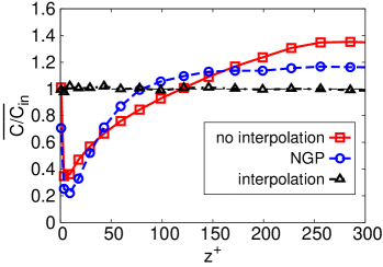
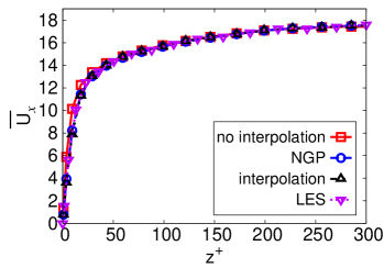
Figure 1: Reynolds-averaged particle number density (a) and filtered streamwise velocity (b), obtained with different SGS particle models: no-interpolation of LES and particle quantities ($\square$), NGP interpolation ($\circ$) and second-order interpolation ($\triangle$). Downward triangles ($\triangledown$) in panel (b) refer to the filtered streamwise velocity provided by LES. The time window for averaging is $\Delta t^{+}=3000$, in wall units.

(a)                                                         (b)

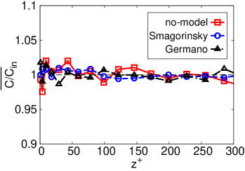
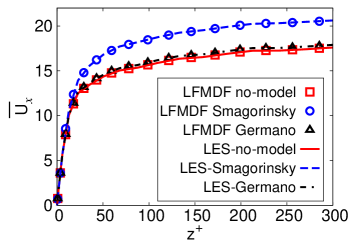
Figure 2: Reynolds-averaged particle number density (a) and filtered streamwise velocity (b), obtained with different SGS models for the fluid: No-model ($\square$, $-$), Smagorinsky model ($\circ$, $--$) and Germano dynamic model ($\triangle$, $-\cdot$). The time window for averaging is $\Delta t^{+}=3000$, in wall units.

(a)                                                         (b)

Figure 1 shows the Reynolds-averaged particle number density, $\overline{C/C_{in}}$ (with $C_{in}$ the number density at the time of particle injection), and particle streamwise velocity, ${\overline{U_{x}}}$ along the wall-normal coordinate. The different profiles correspond to different interpolation techniques. To avoid cross-effects, no subgrid model is used in the Eulerian simulation. While velocity appears unaffected by the particular interpolation technique employed (results are perfectly consistent), particle number density is sensitive. In particular significant errors in the near-wall region are found when no interpolation is performed or when the nearest-grid-point technique is used. A second-order interpolation, however, is sufficient to recover the expected behaviour and ensure $\overline{C/C_{in}}\simeq 1$ everywhere (as expected for tracer particles). In figure 2, the averaged number density profile and the averaged velocity provided by the different SGS models for the fluid are shown. The LFMDF model appears to be consistent with all models tested, since the $\overline{C/C_{in}}$ profile remains uniform once the stationary state is reached and the velocity is (again) perfectly consistent. It is also observed that, in the $\tau_{p}\to 0$ limit, the first moments of the Germano model are nearly the same as those obtained without SGS model. Therefore results discussed hereinafter refer to simulations performed using the Germano model for the fluid phase, unless otherwise stated. A further proof of consistency is provided by figure 3, which shows the scatter plots of the streamwise and wall-normal velocity components, indicated as $\widetilde{U}_{x}$ and $\widetilde{U}_{z}$ respectively. Velocities in the Eulerian simulations were evaluated at the center of the computational cells. The velocity correlation is quite satisfactory, except perhaps for very small values of $\widetilde{U}_{x}$.

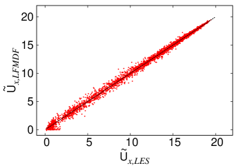
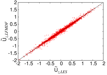
Figure 3: Scatter plot correlating particle velocity components evaluated from LES and from LFMDF: (a) streamwise component, (b) wall-normal component.

(a)                                                          (b)

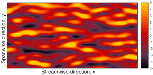
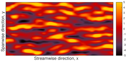
Figure 4: Near-wall fluid velocity streaks. Low-speed (high-speed) streaks are rendered using colored contours of negative (positive) streamwise fluctuating velocity on a horizontal plane at $z^{+}=10$ from the wall. Panel (a) refers to the Eulerian LES, performed with no SGS model for the particles and with $N_{pc}=40$; panel (b) refers to the LFMDF simulation.

(a)

(b)

To assess the consistency of the LFMDF formulation from a physical (and more intuitive) point of view, in Fig. 4, we compare the near-wall fluid streaks that can be rendered from the Eulerian LES (panel a) and from the Monte Carlo LFMDF simulation (panel b). Streaks are known to play a crucial role in determining the transport mechanisms in turbulent boundary layer Picciotto et al. (2005); Marchioli and Soldati (2002), and are visualised here by instantaneous contour plots of the fluctuating streamwise velocity on a $x$-$y$ plane located at a distance $z^{+}=10$ from the wall. Visual inspection shows only small differences in the color map, indicating that the streaks, and indirectly the near-wall turbulent coherent structures that generate it, are indeed recovered by the LFMDF simulation in the fluid limit.

To complete the model assessment, we have also checked the sensitivity of Reynolds averaging to the size of the reference volume $\delta V$ (introduced in Section IV) over which averaging is performed. To this aim, we considered different grids made of cubic volumes centered around the LES (Eulerian) nodes. The size of each volume, $\Delta_{E}$, was varied to be either smaller or larger than the cell size $\Delta$ in the reference $32^{3}$ LES grid. Figure 5 shows the averaged filtered streamwise velocity at varying $\Delta_{E}$ (with a fixed number of particles per cell, $N_{pc}=40$). It can be seen that all profiles overlap even for large $\Delta_{E}$ ($\Delta_{E}=2\Delta$) indicating that the mean filtered velocity is not sensitive to the size of the averaging volume, at least in the range of $\Delta_{E}$ analysed. For this reason we have chosen $\Delta_{E}=\Delta$ for all simulations. To test this choice we have also considered higher-order moments, namely the root mean square (rms) of filtered velocity, and we have analysed the convergence in relation to the DNS results. In figure 6 we show the rms of the filtered velocity, defined as $rms(\tilde{U})=\sqrt{(\overline{\tilde{U}-\overline{\tilde{U}})^{2}}}$. The different profiles do not collapse and the LFMDF is in better agreement than LES with DNS, when the volume size is $\Delta_{E}=\Delta$, confirming the validity of the overall method in the fluid limit. It is worth noting that the discrepancy between Eulerian LES and LFMDF is not related to some incongruity, since these two models are not fully consistent at the Reynolds-stress level. As suggested in previous studies Gicquel et al. (2002), an even better convergence to DNS would be probably possible with smaller $\Delta_{E}$ and much higher $N$. However, this choice would increase the computational cost considerably thus making the model not relevant application-wise.

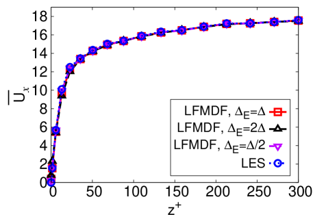
Figure 5: Mean velocity of the filtered streamwise velocity at varying $\Delta_{E}$. Time window for averaging is $\Delta t^{+}=3000$ with $N_{pc}=40$ particle per cell.

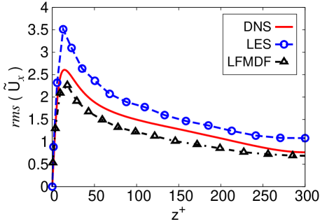
Figure 6: Root mean square of the filtered streamwise velocity.

V.2 Model assessment with inertial particles

In this section we validate the LFMDF approach for the case of inertial particles via comparative assessment against DNS data. In particular, first we exploit DNS to determine the range of empirical constants appearing in the LFMDF sub-model (a priori assessment). Second, we compare the predictions of the LFMDF-based simulations with the statistics provided by DNS, which is regarded here as the reference numerical experiment (a posteriori assessment). In the latter case, comparison is also made with the statistics provided by LES when no particle SGS model is used, in order to point out the impact of the proposed stochastic model on statistics. As mentioned, one of the main difficulties of modelling inertial particle dynamics in LES is to capture preferential concentration Marchioli et al. (2008b, a). Hence, the primary observable considered for comparative assessment is the instantaneous particle number density distribution along the wall-normal direction. Such comparison is particularly severe since any error associated with the proposed particle SGS model will inevitably sum up over time and may thus lead to significant deviations in the final density distribution (we remark here that all LES/LFMDF simulations are carried out with a rather large coarsening factor, $CF=8$ with respect to DNS).

Figure 7 shows the particle number density profiles along the wall-normal coordinate for different Stokes numbers. Two different formulations of the proposed LFMDF model are tested: The simplified LFMDF1 formulation, and the complete LFMDF2 formulation (see Sec. III.4). In both formulations we use $C_{0}=2.1~{},~{}C_{\epsilon}=1$, $\beta=0.8$. The LFMDF1 predictions (dark magenta profiles) deviate substantially from the reference DNS results (red profiles) for all Stokes numbers: This is due, of course, to the assumption of isotropic velocity fluctuations on which the LFMDF1 formulation is based. On the other hand, the LFMDF2 formulation, which has a more complete diffusion term, leads to improved predictions (black profiles), especially for the two larger Stokes numbers: $St=5$, panel (b); and $St=25$, panel (c). Discrepancies, however, are still evident and lead to a significant over-estimation (under-estimation) of particle accumulation in the viscous sub-layer for the smaller $St=1$ (large $St=25$) particles, as shown in Fig. 7(a) and in Fig. 7(c) respectively.

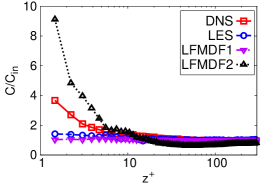
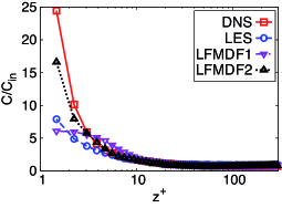
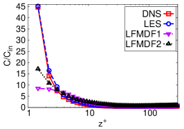
Figure 7: Comparison of particle number density distributions predicted by two different particle SGS model formulations: Simplified stochastic model (LFMDF1, $\triangledown$) and complete stochastic model (LFMDF2, $\triangle$). See also Sec. III.4. Other symbols: $\square$ DNS, $\circ$ LES without particle SGS model. Panels: (a) $St=1$ particles, (b) $St=5$ particles, (c) $St=25$ particles. Profiles are computed at $t^{+}=2130$ after particle injection into the flow.

(a)                                           (b)                                           (c)

The main reason is that the closure of the LMFDF2 formulation involves two parameters, $C_{0}$ and $C_{\epsilon}$, which are known to be quite sensitive to the characteristic features of both the turbulent flow and the numerical approach. For instance, turbulent theory leads to set $C_{0}=2.1$ for stochastic models in homogeneous flows Pope (2000), whereas numerical simulations of wall-bounded flows in the RANS framework suggest to set $C_{0}=3.5$ Minier and Pozorski (1999). In this study, we exploit DNS to obtain a priori estimates of the two model constants. We remark that our purpose is not to find optimal values for $C_{0}$ and $C_{\epsilon}$, but rather to quantify the sensitivity of the model to a change in the value of these constants. Figure 8 shows the number density profiles obtained at varying $C_{0}$ (while keeping $C_{\epsilon}$ constant and equal to 1).

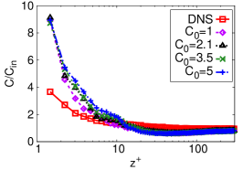
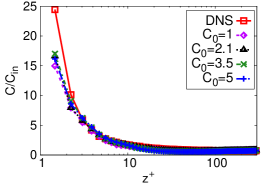
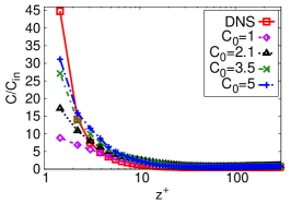
Figure 8: Effect of parameter $C_{0}$ on particle number density along the wall-normal coordinate (a-priori estimate). Red symbols ($\square$) refer to the DNS result, all other symbols refer to LES results obtained with the LFMDF model. Panels: (a) $St=1$, (b) $St=5$, (c) $St=25$. Profiles are computed at $t^{+}=2130$ after particle injection.

(a)                                           (b)                                           (c)

This figure shows that $C_{0}$ has a significant influence on particle wall-normal accumulation only for large-inertia particles (high Stokes numbers), and suggests that $C_{0}=3.5$ provides the best predictions over the range of Stokes numbers considered here. We performed a similar analysis to estimate $C_{\epsilon}$ while keeping $C_{0}$ constant (and equal to 3.5). Results are shown in Fig. 9 and demonstrate that $C_{\epsilon}$ affects particle spatial distribution at all Stokes numbers. In particular, we observe higher accumulation of particles at the wall for smaller values of $C_{\epsilon}$. This finding indicates that the diffusion term is at least as important as the drift term in the present flow configuration. Based on this comparison, we select $C_{\epsilon}=0.1$ to calibrate the LFMDF model.

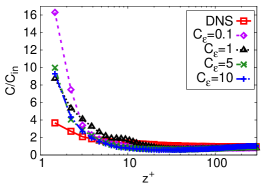
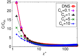
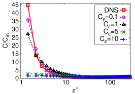
Figure 9: Effect of parameter $C_{\epsilon}$ on particle number density along the wall-normal coordinate (a-priori estimate). Red symbols ($\square$) refer to the DNS result, all other symbols refer to LES results obtained with the LFMDF model. Panels: (a) $St=1$, (b) $St=5$s, (c) $St=25$. Profiles are computed at $t^{+}=2130$ after particle injection.

(a)                                           (b)                                           (c)

A combined analysis of Figs. 8 and 9 indicates that, regardless of the value considered for $C_{0}$ and $C_{\epsilon}$, the near-wall concentration of small inertia particles (represented by the $St=1$ particles in this study) is always overestimated by the LFMDF2 model, whereas the opposite occurred with the LFMDF1 model (see Fig. 7a). For such particles, therefore, the critical modelling issue in order to retrieve the correct physical behaviour seems to be the closure of the diffusion term. We remark here that particles with small inertia are subject to a weaker turbophoretic wallward drift and tend to remain more homogeneously distributed within the flow domain Soldati and Marchioli (2009); Marchioli and Soldati (2002). As a consequence, the instantaneous Eulerian statistics that can be extracted from local particle ensemble averages may exhibit significant statistical errors in the near-wall region, where the control volumes to which averaging is applied become smaller and smaller. This source of error becomes less important as particle inertia increases, namely as particle accumulation in the near-wall region increases with $St$.

The key quantity for a correct evaluation of the diffusion term is the kinetic energy ratio $\widehat{k}_{SGS}/k_{SGS}$. If $\widehat{k}_{SGS}$ is computed from Eq. (24), which implies Lagrangian ensemble averaging, then it will be affected by the resulting statistical error.

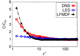
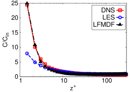
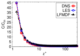
Figure 10: Comparative assessment of the LFMDF model with Eq. (40): Predictions of the instantaneous particle number density at varying Stokes numbers ($\triangle$) are compared with DNS results ($\square$) and with LES results with no particle SGS model ($\circ$). Panels: (a) $St=1$, (b) $St=5$, (c) $St=25$. Profiles are computed at $t^{+}=2130$ after particle injection.

(a)                                           (b)                                           (c)

To improve the model, we propose a new formulation to evaluate $k_{SGS}$, which is slightly different from Eq. (23):

$$k_{SGS}=\tau(U_{s,i},U_{s,i})=\frac{1}{2}\sum_{i=1}^{3}\left[\widetilde{U_{s,i}^{2}}-(\widetilde{U_{s,i}})^{2}\right]~{}.$$ (40)

In the limit of $N_{pc}\to\infty$, Eq. (40) is equivalent to Eq. (24), but is expected to decrease the variance of the model estimations for finite values of $N_{pc}$ at small Stokes numbers. In the following, results for the $St=1$ particles refer to calculations performed using this new formulation, unless otherwise stated. In particular, Fig. 10 shows the comparison of the LFMDF results for particle number density. For completeness, also the LES results without particle SGS model are included. The overshoot of particle accumulation at the wall for $St=1$ is strongly reduced with respect to the predictions reported in Figs. 8 and 9, and there is a nearly perfect match with the DNS profile for the intermediate-inertia particles ($St=5$, Fig. 10b). As expected, wall accumulation at large Stokes numbers is unaffected. We remark that the values of particle number density within a distance of few wall units from the wall are very noisy even in DNS Prevel et al. (2013): This implies that the only relevant information one can extract from the viscous sublayer portion of the profiles shown in Fig. 10 is just the trend in model performance at varying particle inertia.

To provide a phenomenological perspective to our discussion, we complement the statistical description of particle wall-normal distribution with the analysis of particle clustering in the near-wall region. As demonstrated in previous studies (see Marchioli and Soldati (2002); Picciotto et al. (2005); Soldati and Marchioli (2009) and references therein, for a review), the tendency that inertial particles have to form clusters is crucial to develop peaks of particle concentration within the flow. Therefore, a reliable particle SGS model should be able to capture (in a statistical sense) also these phenomena. To perform this analysis, we quantify particle clusters by means of Voronoï diagrams, which represent an efficient and robust tool to diagnose and quantify clustering Monchaux et al. (2010). One Voronoi cell is defined as the ensemble of points that are closer to a given particle than to any other particle in the flow: The area of a Voronoï cell is therefore the inverse of the local particle number density. In addition Voronoï areas are naturally evaluated around each particle and, differently from standard box counting methods, provide a direct measure of particle preferential concentration at inter-particle length scale Monchaux et al. (2010). An example of Voronoï diagram for the present channel flow configuration is shown in Fig. 11, which focuses on the instantaneous distribution of the $St=5$ particles within a wall-parallel fluid slab of thickness $1\leq z^{+}\leq 5$. Only a portion of the $x-y$ plane is shown to highlight the presence of the well-know particle streaks. Compared to the visualisation provided by DNS (Fig. 11a), both LES results (with no particle SGS model in Fig. 11(b); with the LMFDF model in Fig. 11(c), respectively) show broader particle streaks and wider inter-cluster spacing.

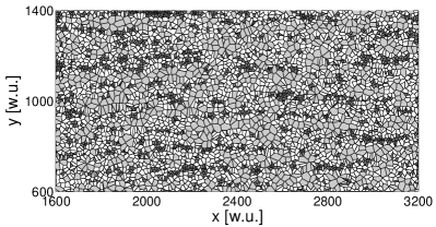
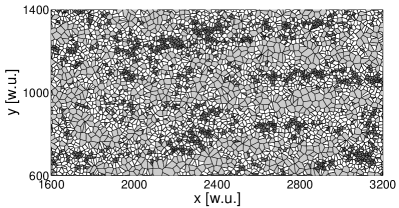
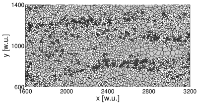
Figure 11: Voronoï tessellation for the $St=5$ particles on a wall-parallel fluid slab ($1\leq z^{+}\leq 5$) at time $t^{+}=2130$ after particle injection. Particle clusters are in dark gray, voids are in ligth gray. Panels: (a) DNS, (b) LES with no particle SGS model, (c) LES with the calibrated LMFDF model.

(a)

(b)

(c)

Clusters and voids are identified by comparing the PDF of Voronoï areas obtained from the simulations to that of a synthetic random Poisson process, whose shape is well approximated by a Gamma distribution Monchaux et al. (2010). This comparison is shown in Fig. 12, where the Voronoï areas are normalized using the average Voronoï area, ${\bar{A}}$ (equivalent to the inverse of the mean particle number density), independent of the spatial organization of the particles.

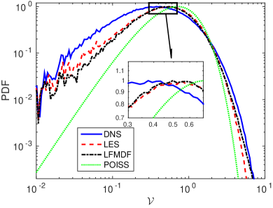
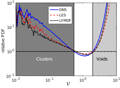
Figure 12: PDF of normalized Voronoï areas ($\mathcal{V}=A/\bar{A}$) of $St=5$ particles on a wall-parallel fluid slab located at distance $1\leq z^{+}\leq 5$ from the wall.

$\mathcal{V}_{c}$      $\mathcal{V}_{v}$

(a)

(b)

As found previously Monchaux et al. (2010), in the case of heavy particles, the PDFs clearly depart from the Poisson distribution, with higher probability of finding depleted regions (large Voronoï areas) and concentrated regions (small Voronoï areas), a typical signature of preferential concentration. In the present study, the inclusion of the LMFDF model into the LES has little effect on the prediction of concentrated regions, and the first cross-over point, $\mathcal{V}_{c}$, representing the threshold value below which Voronoï areas are considered to belong to a cluster, occurs at slightly larger values than in DNS. The model improves prediction of depleted regions even if the second cross-over point, $\mathcal{V}_{v}$, representing the threshold value above which Voronoï areas are considered to belong to a void, is always well predicted.

To complete the LFMDF model assessment, in Fig. 13 we show the statistics of the root mean square of particle velocity. In particular, we focus on the streamwise and wall-normal components, which are the most interesting as far as particle wall transport is concerned. It can be seen that the calibrated LFMDF improves the LES prediction for all Stokes numbers, with just small (yet persistent) discrepancies for the wall-normal rms of the $St=1$ particles (Fig. 13d). This explains the peak of concentration observed for these particles in the number density statistics.

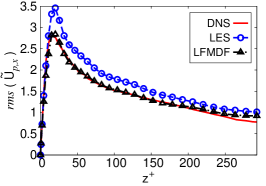
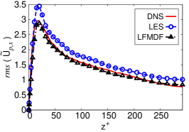
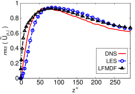
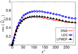
Figure 13: Comparative assessment of the LFMDF model: Prediction of the particle velocity rms at varying Stokes number ($\triangle$) are compared with DNS results (——) and with LES results with no particle SGS model ($\circ$). Panels: (a),(d) $St=1$, (b),(e) $St=5$, (c)-(f) $St=25$; (a)-(c) streamwise component, (d)-(f) wall-normal component. Statistics are obtained averaging over a time window $\Delta t^{+}=1800$.

(a)                                           (b)                                           (c)

(d)                                           (e)                                           (f)

VI Discussion and conclusions

In this work, we have presented a new FDF approach to the simulation of turbulent dispersed flows. The approach is derived from RANS- and LES-based models that have been successfully applied to the simulation of reactive and polydispersed flows Pope (2000); Fox (2012); Peirano et al. (2006). We have put forward a Lagrangian Filtered Mass Density Function (LFMDF) model that provides the Lagrangian probability density function of the SGS particle variables and of the fluid velocity seen by the particles. Important features of the proposed method are that (1) at variance with reactive flows, the approach is Lagrangian and (2) a mass density function is considered, as done in compressible flows. The exact transport equation for the LFMDF has been derived, and a modeled transport equation for the filtered density function has been developed using a closure strategy inspired by PDF methods. Specifically, two different formulations have been proposed, which differ in the treatment of the SGS scales. It has been shown that the effects of convection and polydispersity appear in a closed form.

The modeled LFMDF transport equation has been solved numerically using a Lagrangian Monte Carlo scheme and considering a set of equivalent stochastic differential equations. These equations have been discretized with an unconditionally-stable numerical scheme based on the analytical solution that the equations admit with constant coefficients. This scheme is the natural extension of the one developed in the context of RANS simulations and is the key ingredient for the treatment of multi-scale problems. A turbulent channel flow at shear Reynolds number $Re_{\tau}=300$ based on the channel half height has been simulated and the results yield by the LFMDF method in conjunction with LES have been compared with those provided by large-eddy simulations in which no SGS model is included in the particle equations. To provide a numerical experiment as reference, results from DNS of the same flow configuration have been considered as well. It is important to remark here that Reynolds number effects on the considered statistics are expected to be marginal up to $Re_{\tau}\simeq 900$ Geurts and Kuerten (2012), so that present results can be considered reliable below such threshold value.

The convergence of the Monte Carlo simulations and the consistency of the LFMDF formulation in the fluid-tracer limit have been assessed by comparing particle number density and low-order velocity moments with those obtained from in the purely Eulerian framework. The good agreement of duplicate (Eulerian and Lagrangian) fields demonstrates that the model can safely be applied in the case of particles with small or negligible inertia. We were also able to quantify the effect that the number of particles needed to compute the statistical observables of interest (especially the number density distribution) may have.

The a priori assessment made against DNS allowed us to calibrate the values of the model coefficients for the specific channel flow parameters considered in the present study. Even without dynamic calibration of the coefficients, the a posteriori assessment made against DNS and no-model LES show improved predictions of particle statistics (e.g. particle number density along the wall-normal coordinate and particle velocity fluctuations), especially at intermediate Stokes numbers. In spite of this, however, it should be noted that the LFMDF is a purely statistical method, and therefore can not recover much as far as turbulent coherent structures are concerned.

In our opinion, the LFMDF formulation presented in this paper provides a rigorous and physically-sound approach to the large-eddy simulation of turbulent dispersed flows. While we believe it should be used as the natural framework to develop Lagrangian sub-grid models for the dispersed phase, we are also aware that there is room for further improving the quality and predictive capabilities of the model. A first step would be the development of a dynamic procedure to determine the optimal values of the model coefficients, possibly as a function of the particle Stokes number. Another improvement could be represented by the implementation of higher order closures in the Langevin equation for the fluid velocity seen by the particles. Finally, it would be very useful to implement low-$Re$ corrections to better capture the near-wall behaviour of the statistics: This should improve the model predictions at relatively low particle inertia (e.g. $St=1$ in the present study).

Appendix A Weak first-order Numerical scheme

The analytical solution to the Eqns. (25)-(27) can be obtained with constant coefficients, resorting to Itô’s calculus in combination with the method of the variation of constants. Let us consider the fluid velocity seen by the particles, for instance. One seeks a solution of the form $U_{s,i}(t)=H_{i}(t)\exp(-t/T_{i})$, where $H_{i}(t)$ is a stochastic process defined by (indicating $T_{L,i}^{*}$ with $T_{i}$ for ease of notation):

$$dH_{i}(t)=\exp(t/T_{i})[C_{i}\,dt+\check{B}_{i}\,dW_{i}(t)],$$ (41)

that is, by integration on a time interval $[t_{0},t]$ ($\Delta t=t-t_{0}$),

$$\begin{split}U_{s,i}(t)=U_{s,i}(t_{0})&\exp(-\Delta t/T_{i})+C_{i}\,T_{i}\,[1-\exp(-\Delta t/T_{i})]\\ +&\check{B}_{i}\exp(-t/T_{i})\int_{t_{0}}^{t}\exp(s/T_{i})\,dW_{i}(s),\end{split}$$ (42)

where $\check{B}_{i}=B_{ii}$ since $B_{ij}$ is a diagonal matrix. The derivation of the weak first-order scheme is now rather straightforward since the analytical solutions to Eqns. (25)-(27) with constant coefficients have been already calculated. Indeed, the Euler scheme (which is a weak scheme of order $1$) is simply obtained by freezing the coefficients at the beginning of the time interval $\Delta t=[t_{n},t_{n+1}]$. Let $Z_{i}^{n}$ and $Z_{i}^{n+1}$ be the approximated values of $Z_{i}(t)$ at time $t_{n}$ and $t_{n+1}$, respectively. The Euler scheme is then simply written by using the expression reported in Table 4 and expressing the stochastic integrals through the Choleski algorithm, as reported in Table 5. The second-order scheme is based on a prediction-correction algorithm, in which the prediction step is the first-order scheme of equations (35)-(37) and the corrector step is generated by a Taylor expansion under the assumption that the acceleration terms vary linearly with time Peirano et al. (2006).

Table 4: Analytical solutions to system (27) for time-independent coefficients.

 

$$x_{p,i}(t)=x_{p,i}(t_{0})+U_{p,i}(t_{0})\tau_{p}[1-\exp(-\Delta t/\tau_{p})]+U_{s,i}(t_{0})\,\theta_{i}\{T_{i}[1-\exp(-\Delta t/T_{i})]$$

$$\hskip 25.60747pt+\tau_{p}[\exp(-\Delta t/\tau_{p})-1]\}+[C_{i}\,T_{i}]\{\Delta t-\tau_{p}[1-\exp(-\Delta t/\tau_{p})]-\theta_{i}(T_{i}[1-\exp(-\Delta t/T_{i})]$$

$$\hskip 25.60747pt+\tau_{p}[\exp(-\Delta t/\tau_{p})-1])\}+\Omega_{i}(t)$$ (43)

$$\hskip 25.60747pt\text{\quad with \quad}\theta_{i}=T_{i}/(T_{i}-\tau_{p})$$

$$U_{p,i}(t)=U_{p,i}(t_{0})\exp(-\Delta t/\tau_{p})+U_{s,i}(t_{0})\,\theta_{i}[\exp(-\Delta t/T_{i})-\exp(-\Delta t/\tau_{p})]$$

$$\hskip 25.60747pt+[C_{i}\,T_{i}]\{[1-\exp(-\Delta t/\tau_{p})]-\theta_{i}[\exp(-\Delta t/T_{i})-\exp(-\Delta t/\tau_{p})]\}+\Gamma_{i}(t)$$ (44)

$$U_{s,i}(t)=U_{s,i}(t_{0})\exp(-\Delta t/T_{i})+C_{i}\,T_{i}[1-\exp(-\Delta t/T_{i})]+\gamma_{i}(t)$$ (45)

The stochastic integrals $$\gamma_{i}(t),\;\Gamma_{i}(t),\;\Omega_{i}(t)$$ are given by:

$$\quad\gamma_{i}(t)=\check{B}_{i}\exp(-t/T_{i})\int_{t_{0}}^{t}\exp(s/T_{i})\,dW_{i}(s),$$ (46)

$$\quad\Gamma_{i}(t)=\frac{1}{\tau_{p}}\exp(-t/\tau_{p})\int_{t_{0}}^{t}\exp(s/\tau_{p})\,\gamma_{i}(s)\,ds,$$ (47)

$$\quad\Omega_{i}(t)=\int_{t_{0}}^{t}\Gamma_{i}(s)\,ds.$$ (48)

By resorting to stochastic integration by parts, $$\gamma_{i}(t),\;\Gamma_{i}(t),\;\Omega_{i}(t)$$ can be written:

$$\quad\gamma_{i}(t)=\check{B}_{i}\,\exp(-t/T_{i})\,I_{1,i},$$ (49)

$$\quad\Gamma_{i}(t)=\theta_{i}\,\check{B}_{i}\,[\exp(-t/T_{i})\,I_{1,i}-\exp(-t/\tau_{p})\,I_{2,i}],$$ (50)

$$\quad\Omega_{i}(t)=\theta_{i}\,\check{B}_{i}\,\{(T_{i}-\tau_{p})\,I_{3,i}-[T_{i}\exp(-t/T_{i})\,I_{1,i}-\tau_{p}\exp(-t/\tau_{p})\,I_{2,i}]\},$$ (51)

$$\text{with}\quad I_{1,i}=\int_{t_{0}}^{t}\exp(s/T_{i})\,dW_{i}(s),\quad I_{2,i}=\int_{t_{0}}^{t}\exp(s/\tau_{p})\,dW_{i}(s),\quad I_{3,i}=\int_{t_{0}}^{t}dW_{i}(s).$$

 

Table 5: Derivation of the covariance matrix for constant coefficients.

 

$$\langle\gamma_{i}^{2}(t)\rangle=\check{B}_{i}^{2}\,\frac{T_{i}}{2}\left[1-\exp(-2\Delta t/T_{i})\right]\quad\text{where}\quad\check{B}_{i}^{2}=B_{ii}^{2}$$ (52)

$$\langle\Gamma_{i}^{2}(t)\rangle=\check{B}_{i}^{2}\,\theta_{i}^{2}\left\{\frac{T_{i}}{2}[1-\exp(-2\Delta t/T_{i})]-\frac{2\tau_{p}T_{i}}{T_{i}+\tau_{p}}[1-\exp(-\Delta t/T_{i})\exp(-\Delta t/\tau_{p})]\right.$$

$$\hskip 31.29802pt+\left.\frac{\tau_{p}}{2}[1-\exp(-2\Delta t/\tau_{p})]\right\}$$ (53)

$$\frac{1}{\check{B}_{i}^{2}\,\theta_{i}^{2}}\langle\Omega_{i}^{2}(t)\rangle=(T_{i}-\tau_{p})^{2}\Delta t+\frac{T_{i}^{3}}{2}[1-\exp(-2\Delta t/T_{i})]+\frac{\tau_{p}^{3}}{2}[1-\exp(-2\Delta t/\tau_{p})]$$

$$\hskip 54.06023pt-2T_{i}^{2}(T_{i}-\tau_{p})[1-\exp(-\Delta t/T_{i})]+2\tau_{p}^{2}(T_{i}-\tau_{p})[1-\exp(-\Delta t/\tau_{p})]$$

$$\hskip 54.06023pt-2\frac{T_{i}^{2}\tau_{p}^{2}}{T_{i}+\tau_{p}}[1-\exp(-\Delta t/T_{i})\exp(-\Delta t/\tau_{p})]$$ (54)

$$\langle\gamma_{i}(t)\,\Gamma_{i}(t)\rangle=\check{B}_{i}^{2}\,\theta_{i}\,T_{i}\left\{\frac{1}{2}[1-\exp(-2\Delta t/T_{i})]-\frac{\tau_{p}}{T_{i}+\tau_{p}}[1-\exp(-\Delta t/T_{i})\exp(-\Delta t/\tau_{p})]\right\}$$

$$\langle\gamma_{i}(t)\,\Omega_{i}(t)\rangle=\check{B}_{i}^{2}\,\theta_{i}\,T_{i}\left\{(T_{i}-\tau_{p})[1-\exp(-\Delta t/T_{i})]-\frac{T_{i}}{2}[1-\exp(-2\Delta t/T_{i})]\right.$$

$$\hskip 48.36967pt+\left.\frac{\tau_{p}^{2}}{T_{i}+\tau_{p}}[1-\exp(-\Delta t/T_{i})\exp(-\Delta t/\tau_{p})]\right\}$$ (55)

$$\frac{1}{\check{B}_{i}^{2}\,\theta_{i}^{2}}\langle\Gamma_{i}(t)\,\Omega_{i}(t)\rangle=(T_{i}-\tau_{p})\{T_{i}[1-\exp(-\Delta t/T_{i})]-\tau_{p}[1-\exp(-\Delta t/\tau_{p})]\}$$

$$\hskip 73.97716pt-\frac{T_{i}^{2}}{2}[1-\exp(-2\Delta t/T_{i})]-\frac{\tau_{p}^{2}}{2}[1-\exp(-2\Delta t/\tau_{p})]$$

$$\hskip 73.97716pt+T_{i}\tau_{p}\,[1-\exp(-\Delta t/T_{i})\exp(-\Delta t/\tau_{p})]$$ (56)

The stochastic integrals $$\gamma_{i}^{n},\;\Omega_{i}^{n},\;\Gamma_{i}^{n}$$ are simulated by:

$$\quad\gamma_{i}^{n}=P^{i}_{11}\,{\mathcal{G}}_{1,i},$$

$$\quad\Omega_{i}^{n}=P^{i}_{21}\,{\mathcal{G}}_{1,i}+P^{i}_{22}\,{\mathcal{G}}_{2,i}$$

$$\quad\Gamma_{i}^{n}=P^{i}_{31}\,{\mathcal{G}}_{1,i}+P^{i}_{32}\,{\mathcal{G}}_{2,i}+P^{i}_{33}\,{\mathcal{G}}_{3,i},$$

where $${\mathcal{G}}_{1,i},\;{\mathcal{G}}_{2,i},\;{\mathcal{G}}_{3,i} {\cal N}(0,1)$$ are independent random variables.

The coefficients $$P^{i}_{11},\;P^{i}_{21},\;P^{i}_{22},\;P^{i}_{31},\;P^{i}_{32},\;P^{i}_{33}$$ are defined as:

$$\quad P^{i}_{11}=\sqrt{\langle(\gamma_{i}^{n})^{2}\rangle},$$

$$\quad P^{i}_{21}=\frac{\langle\Omega_{i}^{n}\gamma_{i}^{n}\rangle}{\sqrt{\langle(\gamma_{i}^{n})^{2}\rangle}},\quad P^{i}_{22}=\sqrt{\langle(\Omega_{i}^{n})^{2}\rangle-\frac{\langle\Omega_{i}^{n}\gamma_{i}^{n}\rangle^{2}}{\langle(\gamma_{i}^{n})^{2}\rangle}},$$

$$\quad P^{i}_{31}=\frac{\langle\Gamma_{i}^{n}\gamma_{i}^{n}\rangle}{\sqrt{\langle(\gamma_{i}^{n})^{2}\rangle}},\quad P^{i}_{32}=\frac{1}{P^{i}_{22}}(\langle\Omega_{i}^{n}\Gamma_{i}^{n}\rangle-P^{i}_{21}P^{i}_{31}),\quad P^{i}_{33}=\sqrt{\langle(\Gamma_{i}^{n})^{2}\rangle-(P^{i}_{31})^{2}-(P^{i}_{32})^{2})}.$$

References

- Rogallo and Moin (1984) R. S. Rogallo and P. Moin, Annu. Rev. Fluid Mech. 16, 99 (1984).
- Sagaut (2006) P. Sagaut, Large eddy simulation for incompressible flows: an introduction (Springer Verlag, 2006).
- Lesieur et al. (2005) M. Lesieur, O. Métais, and P. Comte, Large-eddy simulations of turbulence (Cambridge University Press, 2005).
- Smagorinsky (1963) J. Smagorinsky, Mon. Weather Rev. 91, 99 (1963).
- Germano et al. (1991) M. Germano, U. Piomelli, P. Moin, and W. H. Cabot, Phys. Fluids A-Fluid 3, 1760 (1991).
- Germano (1992) M. Germano, J. Fluid Mech. 238, 325 (1992).
- Zamansky et al. (2013) R. Zamansky, I. Vinkovic, and M. Gorokhovski, J. Fluid Mech. 721, 627 (2013).
- Fox (2003) R. O. Fox, Computational models for turbulent reacting flows (Cambridge University Press, 2003).
- Pope (2013) S. B. Pope, P. Combust. Inst. 34, 1 (2013).
- Fox (2012) R. O. Fox, Annu. Rev. Fluid Mech. 44, 47 (2012).
- Armenio et al. (1999) V. Armenio, U. Piomelli, and V. Fiorotto, Phys. Fluids 11, 3030 (1999).
- Yamamoto et al. (2001) Y. Yamamoto, M. Potthoff, T. Tanaka, T. Kajishima, and Y. Tsuji, J. Fluid Mech. 442, 303 (2001).
- Vance et al. (2006) M. Vance, K. Squires, and O. Simonin, Phys. Fluids 18, 063302 (2006).
- Dritselis and Vlachos (2011) C. Dritselis and N. Vlachos, Int. J. Multiphase Flow 37, 706 (2011).
- Afkhami et al. (2015) M. Afkhami, A. Hassanpour, M. Fairweather, and D. Njobuenwu, Comput. Chem. Eng. 78, 248 (2015).
- Kuerten (2006) J. Kuerten, Phys. Fluids 18, 025108 (2006).
- Marchioli et al. (2008a) C. Marchioli, M. Salvetti, and A. Soldati, Phys. Fluids 20, 040603 (2008a).
- Calzavarini et al. (2011) E. Calzavarini, A. Donini, V. Lavezzo, C. Marchioli, E. Pitton, A. Soldati, and F. Toschi, in Direct and Large-Eddy Simulation 8, Ercoftac Series, edited by V. Armenio, B. Geurts, J. Frohlich, and J. G. M. Kuerten (Springer, 2011).
- Fessler et al. (1994) J. R. Fessler, J. D. Kulick, and J. K. Eaton, Phys. Fluids 6, 3742 (1994).
- Wang and Maxey (1993) L. Wang and M. Maxey, J. Fluid Mech. 256, 27 (1993).
- Rouson and Eaton (2001) D. Rouson and J. Eaton, J. Fluid Mech. 428, 149 (2001).
- Soldati and Marchioli (2012) A. Soldati and C. Marchioli, Adv. Water Resour. 48, 18 (2012).
- Soldati and Marchioli (2009) A. Soldati and C. Marchioli, Int. J. Multiphase Flow 35, 827 (2009).
- Picciotto et al. (2005) M. Picciotto, C. Marchioli, and A. Soldati, Phys. Fluids 17, 098101 (2005).
- Balachandar and Eaton (2010) S. Balachandar and J. Eaton, Annu. Rev. Fluid Mech. 42, 111 (2010).
- Marchioli et al. (2008b) C. Marchioli, M. V. Salvetti, and A. Soldati, Acta Mech. 201, 277 (2008b).
- Bianco et al. (2012) F. Bianco, S. Chibbaro, C. Marchioli, M. V. Salvetti, and A. Soldati, Phys. Fluids 24, 045103 (2012).
- Geurts and Kuerten (2012) B. Geurts and J. Kuerten, Phys. Fluids 24, 081702 (2012).
- Chibbaro et al. (2014) S. Chibbaro, C. Marchioli, M. V. Salvetti, and A. Soldati, J. Turbul. 15, 22 (2014).
- Pozorski and Apte (2009) J. Pozorski and S. Apte, Int. J. Multiphase Flow 35, 118 (2009).
- Gobert (2010) C. Gobert, J. Turbul. 11, 1 (2010).
- Shotorban and Mashayek (2005) B. Shotorban and F. Mashayek, Phys. Fluids 17, 081701 (2005).
- Cernick et al. (2015) M. J. Cernick, S. Tullis, and M. Lightstone, J. Turbul. 16, 101 (2015).
- Michałek et al. (2013) W. Michałek, J. Kuerten, J. Zeegers, R. Liew, J. Pozorski, and B. Geurts, Phys. Fluids 25, 123302 (2013).
- Jin et al. (2015) C. Jin, I. Potts, and M. Reeks, Phys. Fluids 27, 053305 (2015).
- Colucci et al. (1998) P. J. Colucci, F. A. Jaberi, P. Givi, and S. B. Pope, Phys. Fluids 10, 499 (1998).
- Jaberi et al. (1999) F. A. Jaberi, P. J. Colucci, S. Givi, and S. B. Pope, J. Fluid Mech. 401, 85 (1999).
- Gicquel et al. (2002) L. Y. Gicquel, P. Givi, F. Jaberi, and S. B. Pope, Phys. Fluids 14, 1196 (2002).
- Sheikhi et al. (2003) M. Sheikhi, T. Drozda, P. Givi, and S. B. Pope, Phys. Fluids (2003).
- Sheikhi et al. (2007) M. Sheikhi, P. Givi, and S. B. Pope, Phys. Fluids 19, 095106 (2007).
- Sheikhi et al. (2009) M. Sheikhi, P. Givi, and S. B. Pope, Phys. Fluids (2009).
- Pope (2000) S. B. Pope, Turbulent flows (Cambridge university press, 2000).
- Lilly (1992) D. K. Lilly, Phys. Fluids A-Fluid 4, 633 (1992).
- Moin and Kim (1982) P. Moin and J. Kim, J. Fluid Mech. 118, 341 (1982).
- Clift et al. (1978) R. Clift, J. R. Grace, and M. E. Weber, Bubbles, Drops and Particles (Academic Press. New York, 1978).
- Minier and Peirano (2001) J.-P. Minier and E. Peirano, Phys. Rep. 352, 1 (2001).
- Minier et al. (2004) J.-P. Minier, E. Peirano, and S. Chibbaro, Phys. Fluids 16, 2419 (2004).
- Minier (2015) J.-P. Minier, Prog. Energ. Combust. 50, 1 (2015).
- Wang and Stock (1993) L.-P. Wang and D. E. Stock, J. Atmos. Sci. 50, 1897 (1993).
- Gardiner (1990) C. W. Gardiner, Handbook of Stochastic Methods for Physics, Chemistry and the Natural Sciences, ed. (Springer-Verlag, Berlin, 1990).
- Minier et al. (2014) J.-P. Minier, S. Chibbaro, and S. B. Pope, Phys. Fluids 26, 113303 (2014).
- Dreeben and Pope (1998) T. D. Dreeben and S. B. Pope, J. Fluid Mech. 357, 141 (1998).
- Wacławczyk et al. (2004) M. Wacławczyk, J. Pozorski, and J.-P. Minier, Phys. Fluids 16, 1410 (2004).
- Peirano et al. (2006) E. Peirano, S. Chibbaro, J. Pozorski, and J.-P. Minier, Prog. Energ. Combust. 32, 315 (2006).
- Marchioli and Soldati (2002) C. Marchioli and A. Soldati, J. Fluid Mech. 468, 283 (2002).
- Muradoglu et al. (1999) M. Muradoglu, P. Jenny, and S. B. Pope, J. Comput. Phys. (1999).
- Jenny et al. (2001) P. Jenny, S. B. Pope, M. Muradoglu, and D. Caughey, J. Comput. Phys. 166, 218 (2001).
- Marchioli et al. (2008c) C. Marchioli, A. Soldati, J. Kuerten, B. Arcen, A. Taniere, G. Goldensoph, K. Squires, M. Cargnelutti, and L. Portela, Int. J. Multiphase Flow 34, 879 (2008c).
- Minier and Pozorski (1999) J.-P. Minier and J. Pozorski, Phys. Fluids 11, 2632 (1999).
- Prevel et al. (2013) M. Prevel, I. Vinkovic, D. Doppler, C. Pera, and M. Buffat, Int. J. Heat Fluid Fl. 43, 2 (2013).
- Monchaux et al. (2010) R. Monchaux, M. Bourgoin, and A. Cartellier, Phys. Fluids 22, 103304 (2010).