Refinements of the Weyl pure geometrical thick branes from information-entropic measure

Abstract

This letter aims to analyse the so-called configurational entropy in the Weyl pure geometrical thick brane model. The Weyl structure plays a prominent role in the thickness of this model. We find a set of parameters associated to the brane width where the configurational entropy exhibits critical points. Furthermore, we show, by means of this information-theoretical measure, that a stricter bound on the parameter of Weyl pure geometrical brane model arises from the CE.

I INTRODUCTION

Recently, the concept of entropy was reintroduced in the literature, by taking into account the dynamical and the informational contents of models with localized energy configurations gleiser-stamatopoulos . Based on the Shannon’s information framework shannon , which represents an absolute limit on the best lossless compression of communication, the Configurational Entropy (CE) was constructed. It can be applied to several nonlinear scalar field models featuring solutions with spatially-localized energy. As pointed out in gleiser-stamatopoulos , the CE can resolve situations where the energies of the configurations are degenerate. In this case, it can be used to select the best configuration. The approach presented in gleiser-stamatopoulos has been used to study the non-equilibrium dynamics of spontaneous symmetry breaking PRDgleiser-stamatopoulos , to obtain the stability bound for compact objects PLBgleiser-sowinski , to study the bounds of Gauss-Bonnet braneworld models rafael-tobias , to explore dynamical holographic AdS/QCD models roldao-alex , to investigate the emergence of localized objects during inflationary preheating PRDgleiser-graham and to distinguish configurations with energy-degenerate spatial profiles as well Rafael-Dutra-Gleiser .

An interesting application of CE occurs in the context of braneworld models, where the parameters of the scenarios can be bounded bc ; Rafael-Pedro ; Rafael-Pedro2 ; Rafael-Davi . In the braneworld perspective, the Randall-Sundrum models RS1 ; RS2 assume that our observable universe is a membrane embedded in an anti-de Sitter five-dimensional spacetime. From this point of view, some prominent results were achieved as the resolution of hierarchy problem RS1 , recovering of Newton’s law RS2 and Coulomb’s law cw2 ; hung ; Davi7 besides many applications to Cosmology and High Energy Physics mc/2016 ; rscosmology ; csaki1 . The recent results in the diphoton experiment by ATLAS LHC1 and CMS LHC2 brought a new phenomenological approach to these braneworld models 750Gev ; Han ; radion ; radion2 ; Csaki2016 . It has also been shown that the braneworld might induce some observational effects in the gravitational wave sign analysis mm/2014 .

In this work, we analyse the CE in the pure geometrical thick brane of Reference Weyl2006 . A manifold endowed with Weyl structure is considered, wherein Weyl scalar employs the thickness of the brane Weyl2006 ; W1 ; W2 . For this reason, the building of these Weyl thick brane models ad1 ; ad2 ; ad3 arise naturally without the necessity of introducing them “by hand”. This procedure preserves the 4D Poincaré invariance and breaks $Z_{2}$-symmetry along the extra dimension. The confinement of gravity in the Weyl brane was performed in Weyl2006 ; W1 ; W2 , while the matter fields in Reference Weyl2006b . Moreover, these pure geometrical thick branes remove the singularities and solve the field non-confinement issues present in Randall-Sundrum thin scenarios Bajc ; 5Dthick .

In the next section of this work, we present a brief review of the Weyl thick brane construction. The concept of CE and its application on the Weyl thick brane are presented in Sec.III. We finish with the results and conclusions in Sec.V.

II Review of pure geometrical Weyl thick brane model

In this section, in order to put our work both in a more pedagogical and comprehensive form in such a way that offers a coherent and credible guide for reader, we will introduce a brief review about pure geometrical Weyl thick brane. Thus, let us begin with the following Weyl (non-Riemannian) action for a pure geometrical 5D scenario Weyl2006

$$S_{5}^{W}=\frac{1}{2\kappa}\int_{M_{5}^{W}}dx^{5}\sqrt{\lvert g\lvert}\operatorname{e}^{\frac{3\omega}{2}}\left[R+3\tilde{\xi}\left(\nabla\omega\right)^{2}+6U(\omega)\right],$$ (1)

where $g$ is the determinant of the metric $g_{MN}$ with $M,N$ running from $1$ to $5$ and $\omega$ represents the Weyl scalar function, which comprise the pair for the Weyl manifold ($M_{5}^{W}$). The constant $\kappa=8\pi G_{5}$ is related to the Newton constant in 5D, $R$ is the scalar curvature, $U(\omega)$ is the self-interacting potential of the scalar field and $\tilde{\xi}$ is an arbitrary parameter which enlarges the class of potentials for which the 4D gravity can be localized. At this point, we would like to emphasize that there are several physical motivations to study the above theory. The first comes from the fact that geometrical thick branes arise naturally without the necessity of introducing them by hand in the action of the theory. In this case, spacetime structures with thick smooth branes separated in the extra dimension arise, where the massless graviton is located in one of the thick branes at the origin, meanwhile the matter degrees of freedom are confined to the other brane. Another remarkable motivation it was introduced by Drechsler refad , where such scenario can generate nonzero masses within the framework of a broken gauge theory containing as a subsymmetry the electroweak gauge symmetry which is known to contain many features in accord with observation.

Assuming for the line element in this 5D geometry an ansatz of the form

$$ds^{2}=\operatorname{e}^{2A(y)}\eta_{\mu\nu}dx^{\mu}dx^{\nu}+dy^{2}\ ,$$ (2)

with $\eta_{\mu\nu}$ being the Minkowski metric with $\mu,\nu$ running from $1$ to $4$, $y$ the fifth dimension, and $A(y)$ the warp factor, the stress-energy tensor components are obtained as Weyl2006 ; W1 ; W2

$$T_{mn}=\frac{3}{\kappa}\operatorname{e}^{2A}\left[A^{\prime\prime}+2\left(A^{\prime}\right)^{2}\right]\eta_{mn},\quad T_{55}=\frac{6}{\kappa}\left(A^{\prime}\right)^{2}\,$$ (3)

with primes indicating derivatives with respect to the extra coordinate.

Now, mapping the Weylian action of Eq.(1) into the Riemannian one through the conformal transformation $\hat{g}_{MN}=\operatorname{e}^{\omega}\eta_{MN}$, we have Weyl2006 ; W1 ; W2

$$S_{5}^{R}=\frac{1}{2\kappa}\int_{M_{5}^{W}}dx^{5}\sqrt{\lvert g\lvert}\left[R+3\xi\left(\hat{\nabla}\omega\right)^{2}+6\hat{U}(\omega)\right]\ ,$$ (4)

where the transformation changes the terms $\xi=\tilde{\xi}-1$ and $\hat{U}(\omega)=\lambda\operatorname{e}^{\frac{4k\xi\omega}{1+k}}U(\omega)$. The metric of Eq.(2) becomes

$$ds^{2}=\operatorname{e}^{\omega(y)}\left[\operatorname{e}^{2A(y)}\eta_{\mu\nu}dx^{\mu}dx^{\nu}+dy^{2}\right]\$$ (5)

in this Riemannian frame.

In order to work with a first order differential system, the authors of Ref.Weyl2006 ; W1 ; W2 write $X=\omega^{\prime}$ and $Y=2A^{\prime}$. Thus, we have the following pair of coupled field equations

$$X^{\prime}+2YX+\frac{3}{2}X^{2} = \frac{1}{\xi}\frac{d\hat{U}}{d\omega}e^{\omega},$$ (6)

$$Y^{\prime}+2Y^{2}+\frac{3}{2}XY = \left(-\frac{1}{\xi}\frac{d\hat{U}}{d\omega}+4\hat{U}\right)e^{\omega}.$$ (7)

Note that the above equations are nonlinear, and unfortunately, as a consequence of the nonlinearity, in general we lose the capability of getting the complete solutions. However, it was shown in Ref. W1 that a special class of analytical solution can be easily obtained with the imposition $X=kY$, where $k\neq 1$ is an arbitrary constant parameter. Thus, both above equations are reduced to the following single differential equation

$$Y^{\prime}+\frac{4+3k}{2}Y^{2}=\frac{4\lambda}{1+k}\operatorname{e}^{\omega\left(\frac{4k\xi}{1+k}+1\right)}\ .$$ (8)

Looking for an alternative solution of Ref.W1 ; W2 , where $\xi=\frac{1-k}{4k}$ and $U=\lambda$ (being $\xi$ determined by arbitraries $k$), the Ref.Weyl2006 sets $\xi=-7/16$, which leads to a potential of the form $U(\omega)=\lambda\operatorname{e}^{-6\omega}$. This potential breaks the invariance under Weyl scaling transformations for arbitrary $\xi\neq 0$ and also transforms the geometrical scalar field into an observable one Weyl2006 . From the impositions of Ref.Weyl2006 the differential equation (8) yields to

$$Y^{\prime}=-12\lambda\operatorname{e}^{-p\omega}\quad\text{or}\quad\omega^{\prime\prime}=16\lambda\operatorname{e}^{-p\omega},$$ (9)

where $p=1+16\xi$, which leads to the relation $A^{\prime}=\frac{3}{8}\omega^{\prime}$.

Hence the functions $A(y)$ and $\omega(y)$ are determined as

$$\operatorname{e}^{2A(y)}=\left\{\frac{\sqrt{-8\lambda p}}{c_{1}}\cosh\left[c_{1}(y-c_{2})\right]\right\}^{\frac{3}{2p}}\ ,\quad\omega(y)=-\frac{2}{p}\ln\left\{\frac{\sqrt{-8\lambda p}}{c_{1}}\cosh\left[c_{1}(y-c_{2})\right]\right\}\ ,$$ (10)

where $c_{1}$ (related to the inverse of warp-factor width) and $c_{2}$ (which is associated to where the warp-factor centering located) are arbitrary integration constants.

Thus, with the $A(y)$ form above, the energy density obtained from $\rho(y)=T_{00}(y)$ is given by

$$\rho(y)=-\frac{9c_{1}^{2}}{4\kappa p}\left\{\frac{\sqrt{-8\lambda p}}{c_{1}}\cosh\left[c_{1}(y-c_{2})\right]\right\}^{\frac{3}{2p}}\left\{1+\frac{3-2p}{2p}\tanh^{2}\left[c_{1}(y-c_{2})\right]\right\}.$$ (11)

For the non-compact extra dimension case (Randall-Sundrum 2 model RS2 ) where $\lambda>0$, $c_{1}>0$ and $p<0$, this quantity will be localized and centered at $c_{2}$, while $c_{1}$ regulates the maximum amplitude of this energy. The thin Randall-Sundrum 2 limit for this distribution is obtained when $p\to-\infty$ and $c_{1}\to\infty$ (provided that $-p/c_{1}$ is finite). It is important to comment that for this scenario the usual $Z_{2}$ symmetry along the $y$ coordinate is not necessarily preserved Weyl2006 . We plot the warp-factor of Eq.(10) and the energy density of Eq.(11) in Fig.1 below.

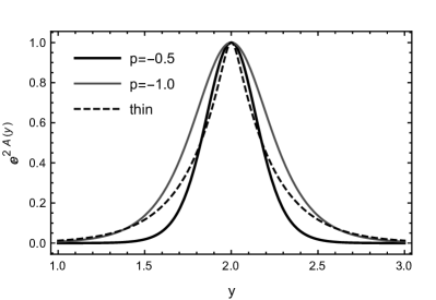
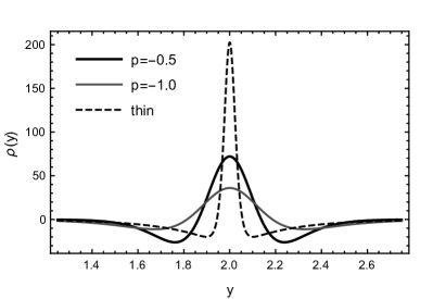
Figure 1: Warp-factor (left) and energy density (right) for the non-compact case. We made $\kappa=1$, $\lambda=-\frac{c_{1}^{2}}{8p}$ and $c_{2}=2$ (which centralized the brane around $y=2$). The thick branes are displayed with $c_{1}=4$ with $p=-0.5$ (thick black line) and $p=-1.0$ (thin grey line). For qualitative thin brane (dashed line) we set $p=-\frac{c_{1}}{3}=-10$.

At this point, it is important to remark that despite having a set of analytical solution, a complete description of the question of bounds on the parameters of the solution, remains an open issue. Then, in the next sections, we seek to address this gap in the literature by finding through of configurational entropy concept a stricter bound on the parameter of these solutions and its physical relevance.

III Configurational Entropy approach

Gleiser and Stamatopoulos gleiser-stamatopoulos have recently proposed a detailed picture of the CE for the structure of localized solutions in classical field theories. In this section, analogously to that work, we formulate a CE measure in the functional space, from the field configurations where the pure geometrical Weyl thick brane scenarios can be studied. Firstly, the framework shall be formally introduced and thereafter its consequences will to be explored.

There is an intimate link between information and dynamics, where the entropic measure plays a prominent role. The entropic measure is well known to quantify the informational content of physical solutions to the equations of motion and their approximations, namely, the CE in functional space gleiser-stamatopoulos . Gleiser and Stamatopoulos proposed that nature optimises not solely by optimising energy through the plethora of a priori available paths, but also from an informational perspective gleiser-stamatopoulos .

To start, let us write the following Fourier transform

$$\mathcal{F}[\Omega]=-\frac{1}{\sqrt{2\pi}}\int dr\;e^{i\Omega r}\mathcal{L},$$ (12)

where $\mathcal{L}$ is the standard Lagrangian density.

Now the modal fraction is defined by the following expression gleiser-stamatopoulos ; PLBgleiser-sowinski ; Rafael-Dutra-Gleiser :

$$f(\Omega)=\frac{\left|\mathcal{F}[\Omega]\right|^{2}}{\int d\Omega\left|\mathcal{F}[\Omega]\right|^{2}}$$ (13)

and measures the relative weight of each mode $\Omega$.

The CE was motivated by the Shannon’s information theory. Indeed, it was originally defined by the expression $S_{C}[f]=-\sum f_{n}\,\ln(f_{n})$, which represents an absolute limit on the best lossless compression of any communication shannon . The CE thus originally provided the informational content of configurations that are compatible to constraints of an arbitrary physical system. When $N$ modes $k$ carry the same weight, then $f_{n}=1/N$ and hence the discrete CE has a maximum at $S_{C}=\ln N$. Instead, if just one mode constitutes the system, then $S_{C}=0$ gleiser-stamatopoulos .

Analogously, for arbitrary non-periodic functions in an open interval, the continuous CE can be described by the expression

$$S_{c}[f]=-\int d\Omega f(\Omega)\ln[f(\Omega)].$$ (14)

Thus, Eq.(12) can be used to generate the normalized fraction, in order to obtain the entropic profile of thick brane solutions. Furthermore, we must find $F(\vec{k})$, defined by the Fourier transform

$$F(\vec{\Omega})=\frac{1}{(2\pi)^{d/2}}\int d^{d}x\;e^{i\vec{\Omega}\cdot{\vec{x}}}\,\rho(\vec{x})\,.\qquad$$ (15)

As we are dealing with one spatial dimension, the above expression reads:

$$F({\Omega})=\frac{1}{\sqrt{2\pi}}\int dx\;e^{i\Omega y}\,\rho({x})\,.$$ (16)

In order to completely specify the normalized fraction $f(\Omega)$, we must calculate $\int\;dk|F(\Omega)|^{2}.$ Hence, by using the Plancherel theorem it follows that

$$\int dk\left|{F}(\Omega)\right|^{2}=\int dx\left|\rho(x)\right|^{2}.$$ (17)

Thus, in the next section, we will apply this new approach to investigate pure geometrical Weyl thick brane theories, which is given by Eq. (1). As we will see, important consequences will arise from the CE concept. Furthermore, we will show that the CE provides a stricter bound on the parameters of the related partial diferential equation (PDE) solution which is represented in Eq. (10).

IV Configurational Entropy in the Weyl Brane

We now use the approach presented in the previous section to obtain the CE of the Weyl brane configurations, which has the set of exact solutions, given in Section II. Let us begin by rewriting the energy density of Eq.(11) in the form

$$\rho(y)=A_{1}\left\{\cosh[c_{1}(y-c_{2})]\right\}^{a}+A_{2}\left\{\cosh[c_{1}(y-c_{2})]\right\}^{b}\left\{\sinh[c_{1}(y-c_{2})]\right\}^{2},$$ (18)

where we are using the following definitions

$$A_{1}\equiv-\frac{9c_{1}^{2}}{4p}\kappa\left(\frac{\sqrt{-8\lambda p}}{c_{1}}\right)^{a},\quad\ A_{2}\equiv A_{1}\left(\frac{6-2p}{2p}\right),$$ (19)

with $a=3/2p$ and $b=3/2p-2$. Thus, we have

$$\mathcal{F}(\Omega)=\int dy\rho(y)e^{i\Omega y}.$$ (20)

In this case, we obtain

$$\mathcal{F}(\Omega)=\frac{e^{i\Omega c_{2}}}{c_{1}}\sum\limits_{m=1}^{2}A_{m}\mathcal{F}_{m}(\Omega),$$ (21)

where

$$\left.\mathcal{F}_{1}(\Omega)=\frac{2^{-a-3/2}i^{a}}{\sqrt{\pi}}\sum\limits_{j=1}^{2}e^{(-1)^{j}\Omega\pi/c_{1}}\beta_{-1}\left[-\frac{a}{2}+\frac{(-1)^{j}\Omega}{2c_{1}},1+a\right],\right.$$ (22)

$$\left.\mathcal{F}_{2}(\Omega)=\frac{2^{-a-5/2}}{\sqrt{\pi}}\left\{2^{b+2}\sum\limits_{j=1}^{2}\frac{1}{b+(-1)^{j+1}ik/c_{1}}H\left[1,1+\frac{b}{2}+\frac{(-1)^{j}i\Omega}{2c_{1}};1-\frac{b}{2}+\frac{(-1)^{j}i\Omega}{2c_{1}};-1\right]\right.\right.$$

$$\left.-\sum\limits_{j=1}^{2}\frac{1}{2+b+(-1)^{j+1}i\Omega/c_{1}}H\left[-b,-1-\frac{b}{2}+\frac{(-1)^{j}i\Omega}{2c_{1}};-\frac{b}{2}+\frac{(-1)^{j}i\Omega}{2c_{1}};-1\right]\right.$$

$$\left.\left.+\sum\limits_{j=1}^{2}\frac{1}{2-b+(-1)^{j+1}i\Omega/c_{1}}H\left[-b,1-\frac{b}{2}+\frac{(-1)^{j}i\Omega}{2c_{1}};2-\frac{b}{2}+\frac{(-1)^{j}i\Omega}{2c_{1}};-1\right]\right\}.\right.$$ (23)

In the above equations, $H[M_{1},M_{2};M_{3;}M_{4}]$ are the hypergeometric functions and $\beta_{-1}(X,Y)$ is the incomplete beta function.

As a result, we plot the normalized fraction in Fig. 3 where we verify that the Weyl parameter $p$ is inversely proportional to the amplitude of $f(\Omega)$. The CE is represented in Fig. 3, where we note that the Weyl parameter decreases the amplitude of the CE. There is a critical point of the CE as a function of the thickness parameter $c_{1}$, as also verified in other thick braneworld models bc ; Rafael-Pedro ; Rafael-Pedro2 ; Rafael-Davi . The evolution of this critical point is represented in Fig.4.

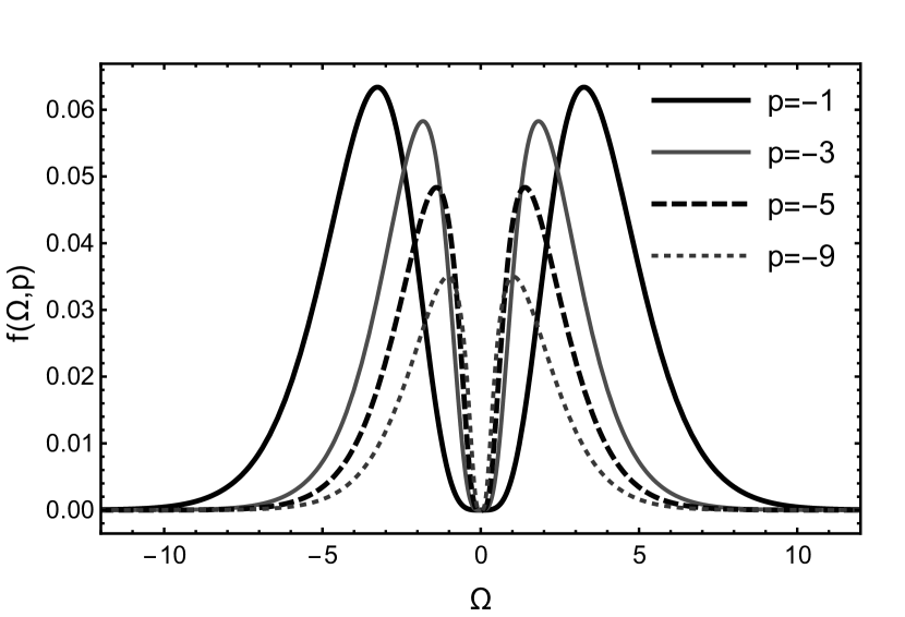
Figure 2: $f(\Omega)$: normalized fraction for the Weyl thick brane as function of associated coupling parameter $p=1+16\xi$. The parameter $p$ regulates the amplitude of $f(\Omega)$.

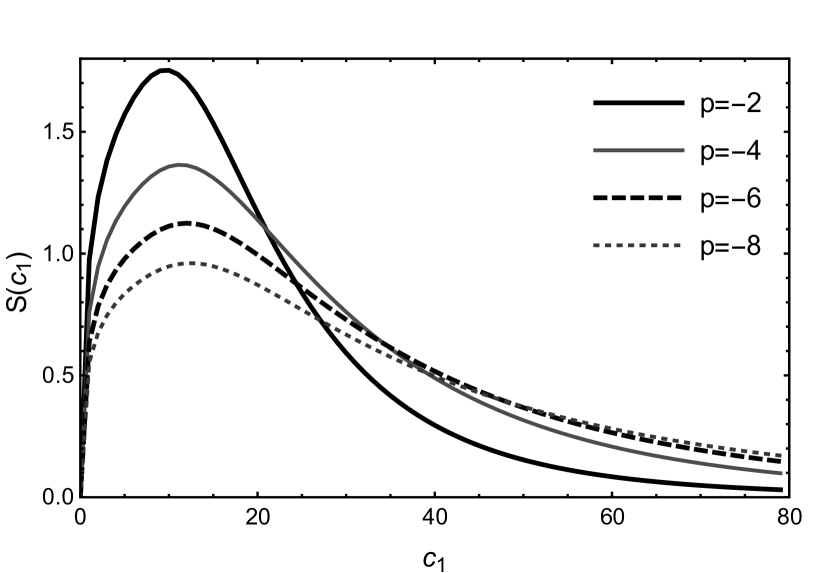
Figure 3: $S(c_{1})$: CE for the Weyl thick brane. When $p\to 0$ and the thin case (where $p\to-\infty$) the CE tends to zero. The CE has a critical maximum detailed in Fig.4.

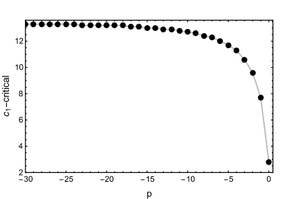
Figure 4: Critical point of CE: when $p\rightarrow-\infty$, $c_{1}\rightarrow 13$.

As we can see, considering the 5-dimensional Weyl gravity model which is given by Eq. (1), it was possible to obtain the information-entropy measure for the system under analysis. Here, it is important to remark that the CE concept states that there is an intimate link between information and dynamics, where entropic measure is responsable in quantify the informational content of physical solutions to the equations of motion and their approximations. In this case, from Fig. 3 we can verify that there is a sharp minimum at the value $c_{1}\rightarrow\infty$, the region of parameter space where the brane solutions are most prominent from the informational point of view. Therefore, in this scenario, the information entropy-measure provide that, when the warp factor of the brane is concentrated near $y=c_{2}$, the corresponding warp factor reproduces the metric of the Randall-Sundrum model in the thin brane limit, showing that the scalar curvature of the Weyl integrable manifold turns out to be completely regular in the extra dimension. Furthermore, at large values of $c_{1}$, the brane-world CE yields the configurational entropy $S_{c}(c_{1})\rightarrow 0$, showing a great organisational degree in the structure of configuration of the system. Finally, by using the approach presented by GS gleiser-stamatopoulos , we have checked that the CE of the configurations given in Section II, is correlated to the energy of the system. The higher [lower] the brane configurational entropy, the higher [lower] the energy of the solutions.

V DISCUSSION and CONCLUSIONS

In this work we performed the analyses of the CE in the Weyl pure geometrical thick brane. This braneworld model was presented in Refs.Weyl2006 ; W1 ; W2 , where the thickness of the model arise from the Weyl scalar fields. These models are subject to some parameter, in special those that regulates the model width as the $c_{1}$ (an arbitrary integration constant) and $p$ (another arbitrary constant associated which is associated to the Weyl coupling parameter $\xi$ Weyl2006 ; W1 ; W2 ).

Applying the CE concept in this model, we conclude that for a fixed $p$ the CE produces a minimum when $c_{1}\rightarrow 0$ (large thickness) and $c_{1}\rightarrow\infty$ (thin limit). On the other hand, a maximum point in the CE is observed for a specific arrangement of the pair $c_{1}$ and $p$. Here, it is important to highlight that our results are consistent with those shown in Rafael-Pedro ; Rafael-Davi ; rrd .

One important physical conclusion that we can draw from our study of the Weyl brane structures, which is given for the model presented in Section II, is the fact that the CE approach can be used to split the solution in two classes. The first one, is given at the values $0<c_{\mathbf{1}}\lesssim 100$, where the configurational entropy measure has values higher than $0$. In this case, the configurational entropy suggest that the Weylian scalar curvature is non–singular along the fifth dimension. On the other hand, when $c_{1}\rightarrow\infty$, the configurational entropy indicates that $S_{c}\rightarrow 0$, and the 5–dimensional curvature scalar is singular. As a consequence, the Randall-Sundrum model is recovered.

Another remarkable result in our analysis comes from the thickness of the domain wall, which is given by the parameter $p$. It is straightforward to realise from Fig. 3 that the higher the brane thickness $p$, the higher the respective value for the brane configurational entropy as well. Moreover, the Weyl brane-world configurational entropy is used to evince a higher organisational degree in the structure of system configuration likewise, for large values of $c_{1}$.

We also intend to study the CE in the six dimensional scenarios of Refs.D1 ; D2 , in addition to those studied in Refs. GS1 ; Torrealba ; D3 ; D4 , presented in the recent work Rafael-Davi .

Acknowledgments

RACC, DMD and CASA thank Coordenação de Aperfeiçoamento de Pessoal de Nível Superior (CAPES), Conselho Nacional de Desenvolvimento Científico e Tecnológico (CNPq) and Fundação Cearense de apoio ao Desenvolvimento Científico e Tecnológico (FUNCAP) for financial support. RACC also acknowledges Universidade Federal do Ceará (UFC) for the hospitality. PHRSM would like to thank São Paulo Research Foundation (FAPESP), grant 2015/08476-0, for financial support.

References

- (1) M. Gleiser and N. Stamatopoulos, Phys. Lett. B 713, 304 (2012).
- (2) C. E. Shannon, The Bell System Technical J. 27, 379 (1948).
- (3) M. Gleiser and N. Stamatopoulos, Phys. Rev. D 86, 045004 (2012).
- (4) M. Gleiser and D. Sowinski, Phys. Lett. B 727, 272 (2013).
- (5) R. A. C. Correa, P. H. R. S. Moraes, A. de Souza Dutra, W. de Paula, and T. Frederico, arXiv:1605.01967.
- (6) A. E. Bernardini and R. da Rocha, arXiv:1605.00294.
- (7) M. Gleiser and N. Graham, Phys. Rev. D 89, 083502 (2014).
- (8) R. A. C. Correa, A. de Souza Dutra, and M. Gleiser, Phys. Lett. B 737, 388 (2014).
- (9) R. A. C. Correa and R. da Rocha, Eur. Phys. J. C 75, 522 (2015).
- (10) R. A. C. Correa, P. H. R. S. Moraes, A. de Souza Dutra, and R. da Rocha, Phys. Rev. D 92, 126005 (2015).
- (11) R. A. C. Correa and P. H. R. S. Moraes, Eur. Phys. J. C 76, 100 (2016).
- (12) R. A. C. Correa, D. M. Dantas, C. A. S. Almeida and R. da Rocha, Phys. Lett. B 755, 358 (2016)
- (13) L. Randall and R. Sundrum, Phys. Rev. Lett. 83, 3370 (1999).
- (14) L. Randall and R. Sundrum, Phys. Rev. Lett. 83, 4690 (1999).
- (15) H. Guo, A. Herrera-Aguilar, Y. X. Liu, D. Malagon-Morejon and R. R. Mora-Luna, Phys. Rev. D 87 (2013) 9, 095011.
- (16) P. Q. Hung and N. K. Tran, Phys. Rev. D 69, 064003 (2004)
- (17) W. T. Cruz, R. V. Maluf, D. M. Dantas and C. A. S. Almeida, arXiv:1512.07890.
- (18) P. H. R. S. Moraes and R. A. C. Correa, Astrophys. Space Sci. 361, 91 (2016).
- (19) T. Clifton, P. G. Ferreira, A. Padilla and C. Skordis, Phys. Rept. 513, 1 (2012)
- (20) C. Csaki, In *Shifman, M. (ed.) et al.: From fields to strings, vol. 2* 967-1060 [hep-ph/0404096].
- (21) The ATLAS collaboration, ATLAS-CONF-2015-081.
- (22) CMS Collaboration [CMS Collaboration], CMS-PAS-EXO-15-004.
- (23) S.B. Giddings and H. Zhang, arXiV:1602.02793v1.
- (24) C. Han, H. M. Lee, M. Park and V. Sanz, Phys. Lett. B 755, 371 (2016).
- (25) H. Davoudiasl and C. Zhang, Phys. Rev. D 93, no. 5, 055006 (2016).
- (26) A. Ahmed, B. M. Dillon, B. Grzadkowski, J. F. Gunion and Y. Jiang, Acta Phys. Pol. B 46, 2205 (2015).
- (27) C. Csaki and L. Randall, arXiv:1603.07303.
- (28) P. H. R. S. Moraes and O. D. Miranda, Astrophys. Space Sci. 354, 645 (2014).
- (29) N. Barbosa-Cendejas and A. Herrera-Aguilar, Phys. Rev. D 73, 084022 (2006) Erratum: [Phys. Rev. D 77, 049901 (2008)]
- (30) O. Arias, R. Cardenas and I. Quiros, Nucl. Phys. B 643, 187 (2002).
- (31) N. Barbosa-Cendejas and A. Herrera-Aguilar, JHEP 0510, 101 (2005).
- (32) C. Romero, J. B. Fonseca-Neto, and M. L. Pucheu, Class. Quantum Grav. 29, 155015 (2012).
- (33) A. Coley, S. Hervik, M. Ortaggio, and L. Wylleman, Class. Quantum Grav. 29 155016 (2012).
- (34) S. Faci, Class. Quantum Grav. 30, 115005 (2013).
- (35) Y. X. Liu, X. H. Zhang, L. D. Zhang and Y. S. Duan, JHEP 0802, 067 (2008)
- (36) B. Bajc, G. Gabadadze, Phys. Lett. B 474, 282 (2000).
- (37) V. Dzhunushaliev, V. Folomeev, and M. Minamitsuji, Rept. Prog. Phys. 73, 066901 (2010).
- (38) W. Drechsler, Found.Phys. 29, 1327 (1999).
- (39) R. A. C. Correa, R. da Rocha, and A. de Souza Dutra, Ann. Phys. 259, 198 (2015).
- (40) D. M. Dantas, J. E. G. Silva, and C. A. S. Almeida, Phys. Lett. B 725, 425 (2013).
- (41) L. J. S. Sousa, C. A. S. Silva, D. M. Dantas, and C. A. S. Almeida, Phys. Lett. B 731, 64 (2014).
- (42) T. Gherghetta and M. E. Shaposhnikov, Phys. Rev. Lett. 85, 240 (2000).
- (43) R. S. Torrealba, Phys. Rev. D 82, 024034 (2010).
- (44) D. M. Dantas, D. F. S. Veras, J. E. G. Silva, and C. A. S. Almeida, Phys. Rev. D 92, 104007 (2015).
- (45) D. M. Dantas, R. da Rocha and C. A. S. Almeida, arXiv:1512.07888.
- (46) M. Gleiser and N. Jiang, Phys. Rev. D 92, 044046 (2015).