Double-difference adjoint seismic tomography

We introduce a ‘double-difference’ method for the inversion for seismic wavespeed structure based on adjoint tomography. Differences between seismic observations and model predictions at individual stations may arise from factors other than structural heterogeneity, such as errors in the assumed source-time function, inaccurate timings, and systematic uncertainties. To alleviate the corresponding nonuniqueness in the inverse problem, we construct differential measurements between stations, thereby reducing the influence of the source signature and systematic errors. We minimize the discrepancy between observations and simulations in terms of the differential measurements made on station pairs. We show how to implement the double-difference concept in adjoint tomography, both theoretically and in practice. We compare the sensitivities of absolute and differential measurements. The former provide absolute information on structure along the ray paths between stations and sources, whereas the latter explain relative (and thus higher-resolution) structural variations in areas close to the stations. Whereas in conventional tomography a measurement made on a single earthquake-station pair provides very limited structural information, in double-difference tomography one earthquake can actually resolve significant details of the structure. The double-difference methodology can be incorporated into the usual adjoint tomography workflow by simply pairing up all conventional measurements; the computational cost of the necessary adjoint simulations is largely unaffected. Rather than adding to the computational burden, the inversion of double-difference measurements merely modifies the construction of the adjoint sources for data assimilation.
Key words: Time-series analysis; Inverse theory; Tomography; Seismic tomography; Computational seismology; Wave propagation.

1 I N T R O D U C T I O N

The quality of tomographic inversions for seismic wavespeed structure is affected by uncertainties in our knowledge of the source-time function (the ‘source wavelet’ in exploration seismology), the (earthquake) source mechanism, location and origin time, inaccuracies in record timekeeping, network geometry, and systematic uncertainties [Nolet (2008)]. All of these factors introduce intrinsic errors into synthetic modeling, even when accurate information on structure is available. Seismic tomography — in seeking to maximize the agreement between simulations and observations from all sources at all recording stations — is at risk of mapping errors of this kind into estimates of wavespeed variations [Schaeffer & Lebedev (2013)]. Jointly updating source terms and structural model parameters [Pavlis & Booker (1980), Spencer & Gubbins (1980), Abers & Roecker (1991), Thurber (1992)], sequentially or iteratively, is a workable albeit expensive solution [Widiyantoro et al. (2000), Panning & Romanowicz (2006), Tian et al. (2011), Simmons et al. (2012)].

The fundamental ideas of making differential measurements were developed early on [[, e.g.]]Brune+63,Passier+95b. The earthquake location community pioneered the concept of ‘double-difference’ inversions [Poupinet et al. (1984), Got et al. (1994)], and a popular code, hypoDD, was introduced by [Waldhauser & Ellsworth (2000)] to improve the accuracy of source locations. The double-difference tomography code tomoDD [Zhang & Thurber (2003)] produces high-resolution wavespeed models simultaneously with accurate event locations. Rather than considering pairs of earthquakes recorded at each station to reduce the effects of structural uncertainty on the source locations, differencing differential measurements between pairs of stations recording the same earthquake lessens the effect of uncertainties in the source terms on the determination of Earth structure [[]]Monteiller+2005,Fang+2014. Much as the double-difference technique has revolutionized earthquake (and other source) studies [[, e.g.]]Rubin+99,Rietbrock+2004,Schaff+2004b, remaining the method of choice for high-resolution hypocenter determination, seismic tomography gains from fully embracing those concepts for structural inversions.

Until now, most of the double-difference approaches have operated within the confines of ray theory [[, but see]]deVos+2013,Maupin+2015. In this paper, we bring double-difference inversions to full-waveform adjoint seismic tomography. Finite-frequency traveltime measurements drive a nonlinear inversion strategy that performs misfit gradient calculations via an elastic adjoint-state method. [Dahlen et al. (2000)] and [Hung et al. (2000)] approximated the Fréchet kernel for differential traveltimes, measured by cross-correlation of phases (e.g., P, S, pP, SS, …) with ‘identical’ pulse shapes, by the difference of the individual single-phase kernels calculated asymptotically. [Hung et al. (2004)] used the same approximation to measure the sensitivities of relative time delays between two nearby stations, which showed improved resolution of the upper-mantle structure beneath a regional array. [Tromp et al. (2005)] brought the elastic adjoint method of [Tarantola (1987), Tarantola (1988)] into global seismology, calculating sensitivity kernels accurately and efficiently using a spectral-element method [Komatitsch & Tromp (2002a), Komatitsch & Tromp (2002b)]. With these techniques it is now possible to incorporate essentially any type of seismic ‘measurement’ (absolute, relative, or differential) into global inversions for seismic wavespeed, boundary perturbations, and source parameters. In this paper, we derive a constructive theory for the incorporation of generic ‘double-difference’ measurements into adjoint seismic tomography.

The minimization of the difference of the difference between observations at distinct pairs of stations, and the difference between synthetics at the same pairs, over all station pairs, requires explicit mathematical expressions for the adjoint sources that are necessary for the numerical computation of the corresponding misfit gradient functionals. We derive those and show in numerical experiments that the gradients of the new misfit functional with respect to structural perturbations are relatively insensitive to an incorrect source signature and timing errors. These results stand in contrast to conventional tomography, which aims to minimize the difference between predictions and observations obtained from measurements made at individual stations.

A seismic phase observed at two ‘nearby’ (relative to the average source-receiver distance) stations will have ‘similar’ (using robust metrics) waveforms and ‘sensitivities’ (misfit gradients) to Earth structure. Station-relative differential measurements will reflect smaller-scale structural variations near to and in-between the station pairs. Structural inversions under the conventional formalism, unless actively ‘re’- or ‘pre’-conditioned to avoid doing so (Curtis & Snieder, 1997; Spakman & Bijwaard, 2001; Fichtner & Trampert, 2011; Luo et al., 2015), tend to over-emphasize areas with high-density ray-path coverage relative to poorly sampled parts of the model. By the partial cancellation of common sensitivities, double-difference tomography, on the contrary, illuminates areas of the model domain where ray paths are not densely overlapping. Hence, using only one event (e.g., a teleseismic earthquake) recorded at a cluster of stations, conventional tomography can derive only very limited structural information, while double-difference tomography will resolve the structure in the instrumented area in greater detail, a benefit that accrues with the density of seismometer arrays Rost & Thomas (2002); Burdick et al. (2014).

The computational cost for tomographic inversion is essentially unaffected by incorporating the double-difference concept into the conventional adjoint tomography workflow. All existing individual measurements are simply paired up, and only the construction of the adjoint sources requires modification. Data assimilation happens by back-propagating all the resulting adjoint sources simultaneously to compute the gradient kernels, exactly as for conventional adjoint tomography, without additional computational burden. Furthermore, the differential measurements themselves can be composed from any of the types used in conventional tomography. For example, they can be relative times calculated from a catalog of absolute arrival times (e.g., VanDecar & Crosson, 1990); they may relative traveltime delays obtained from waveform cross-correlation analysis (e.g., Luo & Schuster, 1991), or from the cross-correlation of their envelopes (e.g., Yuan et al., 2015), and so on. The comparison need not be between the same phase observed at two distinct stations; it can involve different phases recorded on the same trace, or signals recorded at the same station but originating from two different events. In this paper, we use common waveform cross-correlation traveltimes as examples of incorporating differential measurements into adjoint-based tomography. For dispersive waves such as surface waves, differential frequency-dependent phase and amplitude measurements can be made using multitaper cross-spectral analysis. The details of that procedure are relegated to the Appendix.

Double-difference adjoint tomography relies on the assimilation of measurements, which we discuss how to group (e.g., via cluster analysis), and how to weight and stabilize (e.g., by regularization). We propose two approaches to cluster analysis and regularization. The first is based on source-station geometry, in which only station pairs whose spacing is comparable to the scale of the resolvable wavelengths are included in the double-difference data ensemble. The second is based on waveform similarity, as evaluated by the maximum normalized cross-correlation between two waveforms. When the waveform similarity exceeds a certain threshold, the pair of stations is integrated in the double-difference group, and the relative contributions to the misfit function from all qualifying station pairs are weighted by their similarity.

We demonstrate how to make double-difference measurements, and how to use them for adjoint tomography. Numerical experiments show the sensitivities of the double-difference data compared with conventional absolute measurements. We conduct tests with realistic network configurations, both on a global scale and at the scale of the North American continent, and for wavespeed structures that are either checkerboard synthetics or plausible Rayleigh-wave phase speed maps inspired by prior studies.

2 A D J O I N T   T O M O G R A P H Y :   T H E   C L A S S I C A L   A P P R O A C H

We briefly review the principles of ‘conventional’ adjoint tomography using ‘absolute’ cross-correlation traveltimes. The material in this section is later used for comparison with the ‘double-difference’ adjoint tomography using ‘differential’ cross-correlation traveltimes.

The cross-correlation traveltime difference between a synthetic signal $s_{i}(t)$ and an observation $d_{i}(t)$ over a window of length $T$ is defined as

$$\Delta t_{i} =\operatorname*{\arg\!\max}_{\tau}\int_{0}^{T}s_{i}(t+\tau)d_{i}(t)\hskip 1.00006pt\mathrm{d}t,\qquad\mbox{and we define}\qquad\gamma_{i}=\int_{0}^{T}s_{i}(t+\tau)d_{i}(t)\hskip 1.00006pt\mathrm{d}t.$$ (1)

A positive $\Delta t_{i}$ indicates that the data waveform $d_{i}$ is advanced relative to the synthetic $s_{i}$, meaning that the wavespeed model that generated the synthetics is slower than the true model. The objective function to be minimized by ‘least-squares’ is the sum over all measurements of the squared traveltime shifts in eq. (1):

$$\chi_{\tiny\mathrm{cc}} =\frac{1}{2}\sum_{i}[\Delta t_{i}]^{2}.$$ (2)

Explicit and complete derivations for the Fréchet derivatives of the terms in the cross-correlation traveltime misfit function in eq. (2) were presented by various authors (e.g., Luo & Schuster, 1991; Marquering et al., 1999; Dahlen et al., 2000). Most central to the development,

$$\delta\Delta t_{i}=\frac{\int_{0}^{T}\partial_{t}s_{i}(t)\,\delta s_{i}(t)\hskip 1.00006pt\mathrm{d}t}{\int_{0}^{T}\partial^{2}_{t}s_{i}(t)s_{i}(t)\hskip 1.00006pt\mathrm{d}t}.$$ (3)

To turn the expression for the traveltime perturbation, eq. (3), into a useful expression for the perturbation of the misfit function in eq. (2) requires a mechanism to relate a change in Earth properties (density and elastic constants or wavespeeds) to a change in the seismogram, $\delta s_{i}(t)$. Over the years, various formalisms were developed (acoustic, ray-based, modes-based, and numerical approaches), and they were amply discussed in the literature. In addition to the works cited above, we must still mention Zhao et al. (2000), Chen et al. (2007) and Nissen-Meyer et al. (2007). Here we follow Tromp et al. (2005) in taking the numerical approach, which involves the action of an ‘adjoint source’. For an individual measurement of cross-correlation traveltime made at $\mathbf{x}_{i}$, the adjoint source

$$f_{i}^{\dagger}(\mathbf{x},t) =\Delta t_{i}\frac{\partial_{t}s_{i}(T-t)}{\int_{0}^{T}\partial^{2}_{t}s_{i}(t)\,s_{i}(t)\hskip 1.00006pt\mathrm{d}t}\,\delta(\mathbf{x}-\mathbf{x}_{i}).$$ (4)

Note the weighting by the traveltime anomalies $\Delta t_{i}$. The reverse-time synthetics generated at each of the stations from the corresponding adjoint sources in eq. (4) are summed and simultaneously back-propagated. The interaction of the adjoint with the forward-propagating wavefield then produces the gradients of the objective function in eq. (2) with respect to the parameterized model perturbations $m$, leading to expressions that embody the essence of the inverse problem in seismic tomography Nolet (1996), namely

$$\delta\chi_{\tiny\mathrm{cc}}=\int_{\oplus}K_{m}(\mathbf{x})\,m(\mathbf{x})\hskip 1.00006pt\mathrm{d}^{3}\mathbf{x},\quad\mbox{where}\quad K_{m}(\mathbf{x})~{}\mbox{is the cross-correlation traveltime misfit sensitivity kernel for parameter}~{}m.$$ (5)

Positive cross-correlation traveltime differences $\Delta t_{i}$ from eq. (1) result in negative kernel values $K_{m}$ in eq. (5). The model update required is in the direction opposite to $K_{m}$, which, for positive $\Delta t_{i}$ and negative $K_{m}$, implies that the model wavespeeds need to be sped up to reduce the misfit in eq. (2). The integrations are carried out over the entire volume of the Earth, and the summation over the set of parameters $m$ is implied. The typical isotropic situation would be for eq. (5) to involve the density and elastic moduli $\rho(\mathbf{x})$, $\kappa(\mathbf{x})$ and $\mu(\mathbf{x})$, or the density and the elastic wavespeeds $\rho(\mathbf{x})$, $\alpha(\mathbf{x})$ and $\beta(\mathbf{x})$, and so on. Tape et al. (2007), Fichtner et al. (2008), Zhu et al. (2009), and others, describe in detail how the forward and adjoint wavefields interact to produce the various types of ‘misfit sensitivity kernels’ under different model parameterizations, and for the specific case considered in this section. An excellent recent overview is by Luo et al. (2015).

3 A D J O I N T   T O M O G R A P H Y :   T H E   D O U B L E - D I F F E R E N C E   W A Y

We use the term ‘double-difference’ measurement for the difference (between synthetics and observations) of differential measurements (either between pairs of stations or between pairs of events). From the new measurement we construct a new misfit function and derive its Fréchet derivatives and adjoint sources. In this section we focus on ‘measurements’ made by cross-correlation, and take ‘differential’ to mean ‘between pairs of stations, from a common source’. Our definitions can be relaxed later to apply to other types of measurements (e.g., waveform differences, envelope differences), and to refer more broadly to differential measurements, e.g., between different seismic phases or between different seismic sources observed at the same station.

3.1 Measurement

We consider the case of differential traveltimes calculated by cross-correlation of waveforms from a common source recorded at a pair of stations indexed $i$ and $j$. Let $s_{i}(t)$ and $s_{j}(t)$ denote a pair of synthetic waveforms, and let $d_{i}(t)$ and $d_{j}(t)$ be the corresponding pair of observations. The differential cross-correlation traveltimes, between stations, for the synthetic and the observation pairs are, respectively,

$$\Delta t_{ij}^{\mathrm{syn}} =\operatorname*{\arg\!\max}_{\tau}\int_{0}^{T}s_{i}(t+\tau)s_{j}(t)\hskip 1.00006pt\mathrm{d}t,\qquad\mbox{and we define}\qquad\Gamma_{ij}(\tau)=\int_{0}^{T}s_{i}(t+\tau)s_{j}(t)\hskip 1.00006pt\mathrm{d}t,$$ (6a)

$$\Delta t_{ij}^{\mathrm{obs}} =\operatorname*{\arg\!\max}_{\tau}\int_{0}^{T}d_{i}(t+\tau)d_{j}(t)\hskip 1.00006pt\mathrm{d}t,\qquad\mbox{and we define}\qquad\Lambda_{ij}(\tau)=\int_{0}^{T}d_{i}(t+\tau)d_{j}(t)\hskip 1.00006pt\mathrm{d}t.$$ (6b)

A positive $\Delta t_{ij}$ indicates that the waveform recorded at station $j$ (i.e., $s_{j}$ or $d_{j}$) is advanced relative to the waveform recorded at station $i$ (i.e., $s_{i}$ or $d_{i}$). The difference of these differential traveltimes, between synthetics and observations, is the ‘double-difference’ traveltime measurement:

$$\Delta\Delta t_{ij} =\Delta t_{ij}^{\mathrm{syn}}-\Delta t_{ij}^{\mathrm{obs}}.$$ (7)

A positive $\Delta\Delta t_{ij}$ indicates that the advancement of $s_{j}$ over $s_{i}$ is larger than that of $d_{j}$ over $d_{i}$.

3.2 Misfit function

The misfit that we minimize is the sum of squares of the double-difference traveltime measurements, from eq. (7), between all station pairs:

$$\chi_{\tiny\mathrm{cc}}^{\tiny\mathrm{dd}} =\frac{1}{2}\sum_{i}\sum_{j>i}[\Delta\Delta t_{ij}]^{2}.$$ (8)

The summation avoids double counting from the symmetry of the traveltime measurements, since $\Delta t_{ji}^{\mathrm{syn}}=-\Delta t_{ij}^{\mathrm{syn}}$ and $\Delta t_{ji}^{\mathrm{obs}}=-\Delta t_{ij}^{\mathrm{obs}}$.

3.3 Misfit gradient

The derivative of the differential objective function in eq. (8) is

$$\delta\chi_{\tiny\mathrm{cc}}^{\tiny\mathrm{dd}} =\sum_{i}\sum_{j>i}[\Delta\Delta t_{ij}]\,\delta\Delta t_{ij}^{\mathrm{syn}},$$ (9)

where $\delta\Delta t_{ij}^{\mathrm{syn}}$ is the perturbation to the differential traveltime synthetic $\Delta t_{ij}^{\mathrm{syn}}$ caused by a model perturbation. As is customary we approximate the synthetic wavefield in the perturbed model to first order as the sum of the unperturbed wavefield $s(t)$ and a perturbed wavefield $\delta s(t)$,

$$\tilde{s}_{i}(t)=s_{i}(t)+\delta s_{i}(t)\qquad\mbox{and}\qquad\tilde{s}_{j}(t)=s_{j}(t)+\delta s_{j}(t).$$ (10)

Hence, from eqs (6a) and (10), the cross-correlogram of the new seismograms $\tilde{s}_{i}(t)$ and $\tilde{s}_{j}(t)$ is, to first order in the perturbation,

$$\tilde{\Gamma}_{ij}(\tau) =\int_{0}^{T}\tilde{s}_{i}(t+\tau)\tilde{s}_{j}(t)\hskip 1.00006pt\mathrm{d}t\approx\Gamma_{ij}(\tau)+\int_{0}^{T}\delta s_{i}(t+\tau)s_{j}(t)\hskip 1.00006pt\mathrm{d}t+\int_{0}^{T}s_{i}(t+\tau)\delta s_{j}(t)\hskip 1.00006pt\mathrm{d}t=\Gamma_{ij}(\tau)+\delta\Gamma_{i}(\tau)+\delta\Gamma_{j}(\tau).$$ (11)

We introduced the notation $\delta\Gamma_{i}(\tau)$ for the cross-correlogram of $\delta s_{i}(t)$ an $s_{j}(t)$, and $\delta\Gamma_{j}(\tau)$ for that between $s_{i}(t)$ and $\delta s_{j}(t)$, noting that

$$\delta\Gamma_{i}(\tau) =\int_{0}^{T}\delta s_{i}(t+\tau)s_{j}(t)\hskip 1.00006pt\mathrm{d}t=\int_{0}^{T}s_{j}(t-\tau)\delta s_{i}(t)\hskip 1.00006pt\mathrm{d}t\qquad\mbox{and}\qquad\delta\Gamma_{j}(\tau)=\int_{0}^{T}s_{i}(t+\tau)\delta s_{j}(t)\hskip 1.00006pt\mathrm{d}t.$$ (12)

We recall from the definition of the differential cross-correlation traveltime in eq. (6a) that the unperturbed cross-correlogram $\Gamma_{ij}(\tau)$ achieves its maximum at $\tau=\Delta t_{ij}^{\mathrm{syn}}$, in other words, $\partial_{\tau}\Gamma_{ij}(\Delta t_{ij}^{\mathrm{syn}})=0$. If we expand the perturbed cross-correlogram $\tilde{\Gamma}_{ij}(\tau)$ in the vicinity of the unperturbed cross-correlation maximum differential time $\Delta t_{ij}^{\mathrm{syn}}$, keeping terms up to second order, we obtain

$$\tilde{\Gamma}_{ij}(\Delta t_{ij}^{\mathrm{syn}}+\delta\tau) =\Gamma_{ij}(\Delta t_{ij}^{\mathrm{syn}})+\delta\Gamma_{i}(\Delta t_{ij}^{\mathrm{syn}})+\delta\Gamma_{j}(\Delta t_{ij}^{\mathrm{syn}})+\delta\tau\,\partial_{\tau}\delta\Gamma_{i}(\Delta t_{ij}^{\mathrm{syn}})+\delta\tau\,\partial_{\tau}\delta\Gamma_{j}(\Delta t_{ij}^{\mathrm{syn}})+\frac{1}{2}\delta\tau^{2}\>\partial^{2}_{\tau}\Gamma_{ij}(\Delta t_{ij}^{\mathrm{syn}}).$$ (13)

To find the perturbed time shift that maximizes the new cross-correlogram, we set its derivative with respect $\delta\tau$ to zero, thus requiring

$$\partial_{\delta\tau}\tilde{\Gamma}_{ij}(\Delta t_{ij}^{\mathrm{syn}}+\delta\tau) =\delta\tau\,\partial^{2}_{\tau}\Gamma_{ij}(\Delta t_{ij}^{\mathrm{syn}})+\partial_{\tau}\delta\Gamma_{i}(\Delta t_{ij}^{\mathrm{syn}})+\partial_{\tau}\delta\Gamma_{j}(\Delta t_{ij}^{\mathrm{syn}})=0.$$ (14)

The solution then yields the cross-correlation traveltime perturbation $\delta\Delta t_{ij}^{\mathrm{syn}}$ due to the model perturbation, namely

$$\delta\Delta t_{ij}^{\mathrm{syn}} =-\frac{\displaystyle{\partial_{\tau}\delta\Gamma_{i}(\Delta t_{ij}^{\mathrm{syn}})+\partial_{\tau}\delta\Gamma_{j}(\Delta t_{ij}^{\mathrm{syn}})}}{\displaystyle{\partial^{2}_{\tau}\Gamma_{ij}(\Delta t_{ij}^{\mathrm{syn}})}}=\frac{\int_{0}^{T}\partial_{t}s_{j}(t-\Delta t_{ij}^{\mathrm{syn}})\,\delta s_{i}(t)\hskip 1.00006pt\mathrm{d}t-\int_{0}^{T}\partial_{t}s_{i}(t+\Delta t_{ij}^{\mathrm{syn}})\,\delta s_{j}(t)\hskip 1.00006pt\mathrm{d}t}{\int_{0}^{T}\partial^{2}_{t}s_{i}(t+\Delta t_{ij}^{\mathrm{syn}})s_{j}(t)\hskip 1.00006pt\mathrm{d}t}.$$ (15)

We introduce a notation for the denominator,

$$N_{ij}=\int_{0}^{T}\partial^{2}_{t}s_{i}(t+\Delta t_{ij}^{\mathrm{syn}})s_{j}(t)\hskip 1.00006pt\mathrm{d}t,$$ (16)

and rewrite eq. (9), the derivative of the differential cross-correlation objective function in eq. (8), as

$$\delta\chi_{\tiny\mathrm{cc}}^{\tiny\mathrm{dd}} =\int_{0}^{T}\left\{\sum_{i}\left[\sum_{j>i}\frac{\Delta\Delta t_{ij}}{N_{ij}}\partial_{t}s_{j}(t-\Delta t_{ij}^{\mathrm{syn}})\right]\delta s_{i}(t)-\sum_{j}\left[\sum_{i<j}\frac{\Delta\Delta t_{ij}}{N_{ij}}\partial_{t}s_{i}(t+\Delta t_{ij}^{\mathrm{syn}})\right]\delta s_{j}(t)\right\}\mathrm{d}t.$$ (17)

Any scheme by which we minimize eq. (8) proceeds until model perturbations no longer produce meaningful adjustments $\delta\Delta t_{ij}^{\mathrm{syn}}$ in the differential measurement on the synthetics $\Delta t_{ij}^{\mathrm{syn}}$, in which case $\delta\chi_{\tiny\mathrm{cc}}^{\tiny\mathrm{dd}}$ effectively vanishes and a minimum $\chi_{\tiny\mathrm{cc}}^{\tiny\mathrm{dd}}$ is reached.

3.4 Adjoint source

The translation of the gradient expression (17) into an algorithm for which the spectral-element forward-modeling software can be used to produce linearized expressions of the kind in eq. (5) again draws upon the Born approximation and the reciprocity of the Green functions of the wave equation Tromp et al. (2005). An alternative derivation is through the lens of wave-equation constrained functional minimization Liu & Tromp (2006). Either route leads to a paired set of adjoint sources, formulated with respect to the synthetic wavefields $s_{i}$ and $s_{j}$ recorded at locations $\mathbf{x}_{i}$ and $\mathbf{x}_{j}$. Considering all possible such pairs $i$ and $j$, we write the adjoint sources explicitly as

$$f_{i}^{\dagger}(\mathbf{x},t) =+\sum_{j>i}\frac{\Delta\Delta t_{ij}}{N_{ij}}\,\partial_{t}s_{j}\big{(}T-[t-\Delta t_{ij}^{\mathrm{syn}}]\big{)}\delta(\mathbf{x}-\mathbf{x}_{i}),$$ (18a)

$$f_{j}^{\dagger}(\mathbf{x},t) =-\sum_{i<j}\frac{\Delta\Delta t_{ij}}{N_{ij}}\,\partial_{t}s_{i}\big{(}T-[t+\Delta t_{ij}^{\mathrm{syn}}]\big{)}\delta(\mathbf{x}-\mathbf{x}_{j}).$$ (18b)

The comparison of the expression for the adjoint sources of the classical case in eq. (4) with its double-difference counterpart in eqs (18) reveals that the former only involves one waveform per station, whereas in the latter case the adjoint source for each station comprises the waveforms of all the other stations with which it is being compared. As in the classical case, however, the final adjoint source for double-difference measurements is the sum of the contributions from all stations, which are thus back-propagated simultaneously to obtain the adjoint kernels of the objective function in eqs (8). All the pairs of differential measurements are included in the adjoint process, which is otherwise identical to that used in conventional adjoint tomography. Since we linearly combine adjoint sources rather than combining individual adjoint kernels for each data ensemble, only one adjoint simulation is required to numerically evaluate the gradient of the double-difference misfit function, and once again we obtain an expression of the type in eq. (5), with the summation over the parameter type $m$ implied:

$$\delta\chi_{\tiny\mathrm{cc}}^{\tiny\mathrm{dd}}=\int_{\oplus}K^{\tiny\mathrm{dd}}_{m}(\mathbf{x})\,m(\mathbf{x})\hskip 1.00006pt\mathrm{d}^{3}\mathbf{x},\quad\mbox{with}\quad K^{\tiny\mathrm{dd}}_{m}(\mathbf{x})~{}\mbox{the double-difference cross-correlation traveltime misfit sensitivity kernel for}~{}m.$$ (19)

A positive $\Delta\Delta t_{ij}$ defined in eq. (7) results in positive kernel values (19) along the path between the source and station $j$, and negative kernel values along the path towards station $i$. Therefore, to decrease the double-difference misfit function in eq. (8), the model update moves in the negative kernel direction, increasing the wavespeed to station $i$, reducing it towards station $j$, and decreasing the advancement of $s_{j}$ over $s_{i}$.

3.5 Cluster analysis and regularization

From $N$ individual measurements a total of ${{N}\choose{2}}=n(n-1)/2$ double-difference measurements can be created. To enhance the stability of the inverse problem and reduce the computational cost of the data pairings, we can regularize the problem via cluster analysis in which only pairs that are well linked to each other are included. In general this can be achieved by incorporating pairs of stations that are relatively ‘close’, which enhances accuracy and improves tomographic resolution. The maximum separation, however, depends on the wavelength $\lambda$ and the path length $L$ of the phases considered, the scale length of the heterogeneity, and the overall geometry of the illumination of the two stations by seismic sources. In practice a physical distance proportional to $\sqrt{\lambda L}$, the width of the first Fresnel zone, is recommended (e.g., Woodward, 1992; Baig et al., 2003). We can furthermore exclude any station pairs whose spatial offset is much smaller than the expected scale lengths of the structural variations.

Another possible method of clustering is to select station pairs with ‘similar’ signals, as measured by the correlation

$$r_{ij} =\frac{\Lambda_{ij}(\Delta t_{ij}^{\mathrm{obs}})}{\sqrt{\Lambda_{ii}(0)\Lambda_{jj}(0)}},\qquad-1\leq r_{ij}\leq 1,$$ (20)

where we recall the definition of $\Lambda_{ij}$ from eq. (6b). Similarity pairs can be defined on the basis of threshold values for the correlation VanDecar & Crosson (1990), or the squared correlation can be used as weights Waldhauser & Ellsworth (2000). The similarity criterion can be used alone, or in combination with the relative physical proximity of the stations.

4 T H E    A D V A N T A G E   O F   D I F F E R E N T I A L   M E A S U R E M E N T S

In this section we briefly list some of the properties of differential traveltime measurements that make them good candidates for being less affected by source uncertainties than traditional absolute measurements. In the next section, these properties will be verified and illustrated by numerical experiments.

4.1 Scaling invariance

The cross-correlation measurement in eq. (6a) is invariant to scaling of the seismograms $s_{i}(t)$ and $s_{j}(t)$ by a constant factor $\alpha$:

$$\operatorname*{\arg\!\max}_{\tau}\int_{0}^{T}[\alpha s_{i}(t+\tau)][\alpha s_{j}(t)]\hskip 1.00006pt\mathrm{d}t=\operatorname*{\arg\!\max}_{\tau}\left[\alpha^{2}\int_{0}^{T}s_{i}(t+\tau)s_{j}(t)\hskip 1.00006pt\mathrm{d}t\right]=\operatorname*{\arg\!\max}_{\tau}\int_{0}^{T}s_{i}(t+\tau)s_{j}(t)\hskip 1.00006pt\mathrm{d}t=\Delta t_{ij}^{\mathrm{syn}}.$$ (21)

The scale invariance directly removes any sensitivity to incorrect seismic moment estimates.

4.2 Shift invariance

The time shift calculated by maximizing the cross-correlogram in eq. (6a) is unchanged if time is globally shifted by some constant $\tau_{0}$:

$$\operatorname*{\arg\!\max}_{\tau}\int_{0}^{T}s_{i}(t+\tau-\tau_{0})\>s_{j}(t-\tau_{0})\hskip 1.00006pt\mathrm{d}t=\operatorname*{\arg\!\max}_{\tau}\int_{0}^{T}s_{i}(t+\tau)\;s_{j}(t)\hskip 1.00006pt\mathrm{d}t=\Delta t_{ij}^{\mathrm{syn}}.$$ (22)

The shift invariance directly removes any sensitivity to errors in origin time.

4.3 Source wavelet invariance

Knowledge of the source-time-function or ‘wavelet’ is of course crucial to making accurate measurements. Differential measurements, from the same seismic event to a pair of stations, are more robust to errors in the source wavelet than absolute ones. They should also be relatively robust to errors in the source’s focal mechanism, unless incorrect assumptions should place one of the event-station paths — but not both — on the wrong side of the nodal plane. The cross-correlation time delays between two synthetic seismograms calculated with the wrong source information should be relatively robust as long as we can view the ‘wrong’ records as filtered, or otherwise mostly linearly mapped, from what would be the ‘right’ seismograms. As long as the phases targeted by the cross-correlation time window remain well separated temporally from neighboring phases, in either case, they could be remapped to the same impulsive arrivals after deconvolution of their respective input source wavelets, hence preserving the differential delay time.

4.4 Differential sensitivity versus sensitivity of differential measurement

Eq. (15) contains two terms that contribute to the traveltime sensitivity, the Fréchet derivatives for the differential cross-correlation traveltime. Both of these mix contributions from both seismograms $s_{i}$ and $s_{j}$. Now suppose waveforms of $s_{i}(t)$ and $s_{j}(t)$ are identical upon time shifting, i.e., they are of the ‘identical pulse shape’ type (perhaps achieved by pre-processing, e.g., to equate the Maslov indices of P and PP, or S and SS) as identified by Dahlen et al. (2000). In that case

$$s_{i}(t)\approx s_{j}(t-\Delta t_{ij}^{\mathrm{syn}})\qquad\mbox{and}\qquad s_{j}(t)\approx s_{i}(t+\Delta t_{ij}^{\mathrm{syn}}),$$ (23)

and in that case eq. (15) would reduce to a form that does not mix station indices, and we learn by comparison with eq. (3) that

$$\delta\Delta t_{ij}^{\mathrm{syn}}=\frac{\int_{0}^{T}\partial_{t}s_{i}(t)\delta s_{i}(t)\hskip 1.00006pt\mathrm{d}t}{\int_{0}^{T}\partial^{2}_{t}s_{i}(t)s_{i}(t)\hskip 1.00006pt\mathrm{d}t}-\frac{\int_{0}^{T}\partial_{t}s_{j}(t)\delta s_{j}(t)\hskip 1.00006pt\mathrm{d}t}{\int_{0}^{T}\partial^{2}_{t}s_{j}(t)s_{j}(t)\hskip 1.00006pt\mathrm{d}t}=\delta\Delta t_{i}-\delta\Delta t_{j}.$$ (24)

In other words, in the case of ‘identical’ waveforms, the Fréchet sensitivity kernel for their differential traveltime can be approximated by taking the difference of the individual Fréchet sensitivity kernels for each of the absolute traveltimes, and the classical formalism of adjoint tomography can be used to perform double-difference adjoint tomography, albeit approximately. This is the approach adopted by, among others, Hung et al. (2004).

Conditional statements of the kind that validated the applicability of eq. (24) for using differential phases (either for different phases at the same station, or from the same phase at different stations) were made by Dahlen et al. (2000) (compare our eq. 15 with their eq. 75). These assumptions are, however, not generally valid. In contrast, our eqs (18) are proper generalizations of the differential traveltime adjoint sources of Tromp et al. (2005) (their eq. 61) which do not suffer similar such restrictions — save for the general adequacy of the Born approximation, which appears practically unavoidable though perhaps not theoretically unassailable Hudson & Heritage (1981); Panning et al. (2009); Wu & Zheng (2014).

As a further point of note, it is computationally more efficient and algorithmically less complicated to evaluate the double-difference adjoint kernel using eqs (18) than via eqs (4) and (24). For example, for a total number of $N$ measurements, one only needs one adjoint simulation to numerically calculate the gradient of the differential misfit under ${{N}\choose{2}}$ possible combinations. In contrast, by using the approximation in eq. (24), one needs to compute the Fréchet sensitivity kernel for each individual measurement, which requires $N$ adjoint simulations in total. Subsequently these sensitivity kernels need to be combined by weighted with the corresponding double-difference traveltime measurements, and summed up for all grouped kernels. In conclusion, the misfit sensitivity for differential measurements for use in double-difference adjoint tomography is best obtained, both theoretically and in practice, via the paired adjoint sources of eqs (18).

5 N U M E R I C A L   E X P E R I M E N T S

Three types of validation experiments are conducted here. We consider input checkerboard patterns but also a realistic phase speed distribution, for sensor configurations that proceed in complexity from two stations to simple arrays, and then to realistic array configurations.

5.1 Checkerboard model tests, local networks

We first conduct a numerical experiment with strong lateral heterogeneity, with a 2-D ‘checkerboard’ input model as shown in Fig. 1. We use membrane surface waves Tanimoto (1990); Peter et al. (2007) as an analogue for short-period (10–20 s) surface waves. We use SPECFEM2D Komatitsch & Vilotte (1998) to model the wavefield. Absorbing boundary conditions are employed on all sides.

Experiment I, as shown in Fig. 1, involves one source (filled star), and two stations (open circles labeled 1 and 2) that are aligned at different epicentral distances along a common source-receiver ray path. The target model of interest is a 480 km $\times$ 480 km checkerboard expressed as four circular S-wave speed anomalies of alternating sign, shown in Fig. 1a. The initial model is a featureless homogeneous model with S-wave speed of 3500 m/s, shown in Fig. 1b. We uniformly discretize each dimension using 40 elements of individual length 12 km. The source wavelet used is the first derivative of a Gaussian function with a dominant period of 12 s. The sampling rate is 0.06 s and the total recording length is 4.8 s. The exact source-time function and event origin time were used in the computation.

Fig. 2a and Fig. 2b show the displacement seismograms recorded at stations 1 and 2, respectively. The black traces marked ‘data’ are calculated in the checkerboard model of Fig. 1a. The green traces labeled ‘synthetic’ are predictions in the homogeneous model of Fig. 1b. We evaluate the time shift between the predictions (green) and the observations (black) at each of the stations via the conventional cross-correlation approach, as in eq. (1). These measurements are $\Delta t_{1}=4.08$ s ($d_{1}$ is advanced 4.08 s relative to $s_{1}$) and $\Delta t_{2}=6.60$ s ($d_{2}$ is advanced 6.60 s relative to $s_{2}$). Following eq. (2) in this example, the objective function is the sum of the squares of the individual time shifts $\chi_{\tiny\mathrm{cc}}=\frac{1}{2}([\Delta t_{1}]^{2}+[\Delta t_{2}]^{2})=30.1$ s². Fig. 2c and Fig. 2d show the adjoint sources calculated from eq. (4), in non time-reversed coordinates, as blue lines labeled ‘cc’.

The double-difference cross-correlation approach measures, via eq (6a), the time shift between the predictions made at station 1 and 2 (green traces in Figs 2a–b) and, via eq. (6b), between the observations at those same stations (black lines in Figs 2a–b). The first of these is $\Delta t_{12}^{\mathrm{syn}}=-32.34$ s ($s_{2}$ is delayed 32.34 s relative to $s_{1}$), and the second $\Delta t_{12}^{\mathrm{obs}}=-29.76$ s ($d_{2}$ is delayed 29.76 s relative to $d_{1}$). Their ‘double’ difference, from eq. (7), yields $\Delta\Delta t_{12}=-2.58$ s (the delay of $s_{2}$ over $s_{1}$ is 2.58 s larger than that of $d_{2}$ over $d_{1}$). The double-difference objective function of eq. (7) is the sum of the squared double differences over all available pairs, which in this case simply evaluates to $\chi_{\tiny\mathrm{cc}}^{\tiny\mathrm{dd}}=\frac{1}{2}[\Delta\Delta t_{12}]^{2}=3.33$ s². Fig. 2c and Fig. 2d show the adjoint sources calculated from eqs (18a) and (18b), again in natural time coordinates, as red lines, which are labeled ‘cc_dd’.

Fig. 3 shows the misfit sensitivity kernels for both types of measurements. The cross-correlation traveltime S-wave speed adjoint misfit kernel $K_{\beta}(\mathbf{x})$ shown in Fig. 3a is most sensitive to the area of effective overlap of the ray paths from the source to either station. This behavior is indeed explained by the nature of the kernel, which is obtained by summation of the individual adjoint kernels for each station. The desired model update is in the opposite kernel direction, increasing the wavespeed to station 1 and to station 2. In contrast, the double-difference cross-correlation traveltime S-wave speed adjoint misfit kernel $K^{\tiny\mathrm{dd}}_{\beta}(\mathbf{x})$ shown in Fig. 3b displays a dominant sensitivity in the area in-between the two stations. The ‘double’ differencing of the traveltime metrics between the distinct stations, cancels out much of the sensitivity common to both ray paths, the area between the source and station 1 in this case. The traveltime delay of the waves recorded at station 2, relative to station 1, mainly reflects the average S-wave speed between stations 1 and 2. The finite-frequency character of the measurements remains apparent from the ‘swallowtails’ visible in the area between the source and station 1. The opposite kernel direction required for model update is to slow down along the path from the source to station 1, and to speed up towards station 2. Since the path of station 1 overlaps that of station 2, the resulting effect is to increase the wavespeed between station 1 and station 2.

Experiment II, as shown in Fig. 4, again involves one source (filled star) and two stations (open circles), but now the latter have been arrange to lie at the same epicentral distance but at different azimuthal directions relative to the source.

In Experiment IIA we consider the ideal situation when source information is known. The exact timing and the exact source wavelet (again, the first derivative of a Gaussian with dominant period of 12 s) are used for synthetic modeling. Fig. 5a and Fig. 5b show the displacement seismograms recorded at both stations, with the checkerboard-model traces in black and the homogeneous-model traces in green. The cross-correlation time shift measurements are now $\Delta t_{1}=0.54$ s ($d_{1}$ is advanced 0.54 s relative to $s_{1}$) and and $\Delta t_{2}=-0.54$ s ($d_{2}$ is delayed 0.54 s relative to $s_{2}$). These are small and almost identical as the ray paths sample almost equal path lengths of slow and fast wavespeed anomalies. Fig. 5c and Fig. 5d show the adjoint sources for this model setup. In blue, for the traditional cross-correlation time shift between predictions and observations, in red for the difference of the differential cross-correlation time shifts between stations, where $\Delta t_{12}^{\mathrm{syn}}=0.00$ s (as $s_{1}$ and $s_{2}$ arrive at the same time), $\Delta t_{12}^{\mathrm{obs}}=-1.08$ s (as $d_{2}$ is delayed by 1.08 s relative to $d_{1}$), and the ‘double’ difference $\Delta\Delta t_{12}=1.08$ s. Fig. 6 shows the misfit sensitivity kernels for both types of adjoint measurements.

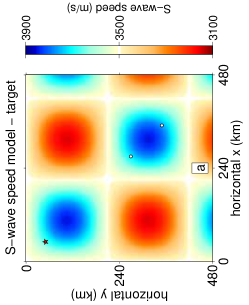
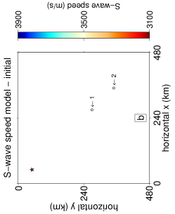
Figure 1: Experiment I: model configuration. Two stations at different epicentral distances located along a common source-receiver path. (a) Target wavespeed model. (b) Initial model. The source is depicted by a filled star. The open circles are stations $i=1$ and $j=2$.

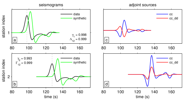
Figure 2: Experiment I: data and synthetics. (a–b) Displacement seismograms, (a) at station $i=1$ and (b) at station $j=2$. The black traces are the ‘data’, computed in the target model shown in Fig. 1a. The green traces are the ‘synthetics’, calculated in the initial model shown in Fig. 1b. Cross-correlation traveltimes, computed via eq. (1), are $\Delta t_{1}=4.08$ s and $\Delta t_{2}=6.60$ s. The offset between the traces in panels (a) and (b) is $\Delta t_{12}^{\mathrm{obs}}=-29.76$ s for the observations and $\Delta t_{12}^{\mathrm{syn}}=-32.34$ s for the predictions, calculated via eq. (6). (c–d) Adjoint sources, (c) at station $i=1$ and (d) at station $j=2$. The blue traces marked ‘cc’ are calculated via eq. (4) and correspond to the conventional cross-correlation metrics $\Delta t_{1}$ and $\Delta t_{2}$, rendered to scale. The red traces marked ‘cc_dd’ are calculated via eq. (18) and correspond to the double-difference cross-correlation metric $\Delta t_{12}^{\mathrm{syn}}-\Delta t_{12}^{\mathrm{obs}}=\Delta\Delta t_{12}=-2.58$ s, to scale.

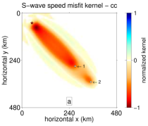
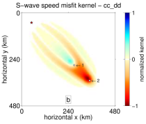
Figure 3: Experiment I: misfit sensitivity kernels. (a) Cross-correlation traveltime misfit sensitivity kernel $K_{m}(\mathbf{x})$, as in eq. (5), computed using the adjoint sources shown by the blue lines in Fig. 2c–d. (b) Double-difference cross-correlation traveltime misfit sensitivity kernel $K_{m}^{\tiny\mathrm{dd}}(\mathbf{x})$, as in eq. (19) computed using the adjoint sources shown by the red lines in Fig. 2c–d. In both cases, the parameter of interest is $m=\beta$, the S-wave speed.

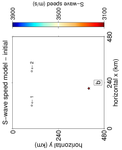
Figure 4: Experiment II: model configuration. Two stations (open circles) at the same epicentral distance but with different azimuthal directions with respect to the source (filled star). (a) Target wavespeed model. (b) Initial model.

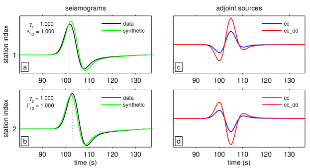
Figure 5: Experiment IIA: data and synthetics. (a–b) Displacement seismograms at stations 1 and 2. Black traces are computed in the target model of Fig. 4a. Green traces are for the initial model in Fig. 4b. The correct source-time function and origin time are being used. Cross-correlation traveltimes $\Delta t_{1}=0.54$ s and $\Delta t_{2}=-0.54$ s. Double-difference measurements $\Delta t_{12}^{\mathrm{obs}}=-1.08$ s, $\Delta t_{12}^{\mathrm{syn}}=0.00$ s, hence $\Delta\Delta t_{12}=1.08$ s. (c–d) Adjoint sources. Blue traces are for the conventional cross-correlation (‘cc’) adjoint source (4). Red traces are for the double-difference cross-correlation (‘cc_dd’) adjoint source (18).

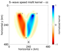
Figure 6: Experiment IIA: misfit sensitivity kernels. (a) Adjoint kernel $K_{\beta}(\mathbf{x})$ corresponding to the adjoint sources (blue lines) in Fig. 5c–d. (b) Double-difference adjoint kernel $K_{\beta}^{\tiny\mathrm{dd}}(\mathbf{x})$ from the adjoint sources (red lines) in Fig. 5c–d. The kernels look very similar but their role and interpretation are different.

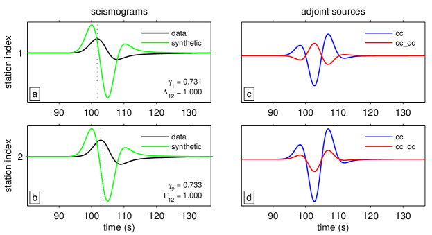
Figure 7: Experiment IIB: data and synthetics. (a–b) Displacement seismograms, computed in the target model (black) and in the initial model (green). An incorrect source model was used in the latter case (different source-time function but the same origin time and dominant periods). Cross-correlation traveltimes $\Delta t_{1}=-2.64$ s and $\Delta t_{2}=-3.72$ s. Double-difference measurements $\Delta t_{12}^{\mathrm{obs}}=-1.08$ s, $\Delta t_{12}^{\mathrm{syn}}=0.00$ s, thus $\Delta\Delta t_{12}=1.08$ s. (c–d) Adjoint sources for the conventional cross-correlation (blue) and for the double-difference cross-correlation (red).

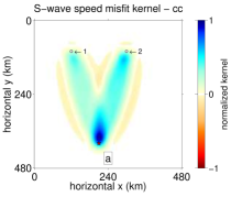
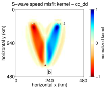
Figure 8: Experiment IIB: misfit sensitivity kernels. (a) Conventional adjoint kernel $K_{\beta}(\mathbf{x})$ and (b) double-difference adjoint kernel $K_{\beta}^{\tiny\mathrm{dd}}(\mathbf{x})$ from the adjoint sources shown in Fig. 7c–d. The kernels are very different from one another. Since the wrong source-time function was used, the cross-correlation traveltime misfit kernel in (a) differs greatly from the one in Fig. 6a, whereas the double-difference misfit kernel in (b) is almost identical to the one shown in Fig. 6b.

The $K_{m}(\mathbf{x})$ and $K_{m}^{\tiny\mathrm{dd}}(\mathbf{x})$ kernels, at first glance, look very similar, but their physical meanings are very different. The traditional measurements provide absolute information on wavespeed structure along the ray paths, whereas the double-difference measurements are sensitive to relative structural variations. From the classical prediction-observation cross-correlation measurements, we learn that the surface waves predicted to be recorded at station 1 arrive 0.54 s later than the observations, and those predicted at station 2 arrive 0.54 s earlier than the observations. To reduce the misfit function (in eq. 2), the wavespeed along the ray path from the source to station 1 should be increased, and the wavespeed between the source and station 2 decreased. On the other hand, from the differential cross-station traveltime measurements, we deduce that there is a 1.08 s advance in the arrival of the observed waves at station 1 relative to station 2, but the synthetic records arrive at exactly the same time at both stations, based on the lag time of their cross-correlation maximum. Of course here too, to reduce the misfit (in eq. 8), the wavespeed from the common source to station 1 should be made faster than that to station 2.

In Experiment IIB we treat the more realistic scenario where an incorrect source wavelet is used for the synthetic modeling. Fig. 7a and 7b show the displacement synthetics. The observations (black) are in the checkerboard model and use the first derivative of the Gaussian function for a source wavelet. The predictions (green) use the second derivative of the Gaussian, the ‘Ricker’ wavelet. Both source wavelets share the same excitation time and dominant period of 12 s. The cross-correlation time shifts between the synthetics and observations are $\Delta t_{1}=-2.64$ s and $\Delta t_{2}=-3.72$ s. These are markedly different from the measurements obtained above using the correct source wavelet (recall those were $\Delta t_{1}=0.54$ s, $\Delta t_{2}=-0.54$ s). In contrast, the double-difference time shift between station 1 and station 2 is unchanged from that which uses the correct source wavelet, $\Delta\Delta t_{12}=1.08$ s. Fig. 8 shows the misfit kernels.

The effects of an incorrect source signature on the traditional cross-correlation measurements can be clearly seen by comparing the adjoint kernel in Fig. 8a with that shown in Fig. 6a. These are markedly different. Fortunately, the double-difference measurement approach yields relatively consistent adjoint kernels, based on the comparison of the kernel shown in in Fig. 8b with the one using exact source signature in Fig. 6b. The latter two are nearly identical, which is indicative of desirable robustness in the inversion.

In Experiment IIC we next consider the scenario of having an incorrect origin time, an advance of 0.96 s expressed by the synthetics. Fig. 9a and Fig. 9b show the records, with the same color conventions as before. It comes as no surprise that the cross-correlation time shifts between predictions and observations are biased. We obtain $\Delta t_{1}=-0.42$ s and $\Delta t_{2}=-1.50$ s, a spurious shift of 0.96 s for each measurement. The differential cross-correlation time shifts between stations, however, are not affected at all, since the predictions at both stations, wrong as they both are, are shifted in exactly the same way with respect to the true source origin time. Fig. 10 shows the misfit kernels. The conventional cross-correlation kernel, in Fig. 10a, are clearly affected by the timing error, while the double-difference ones, in Fig. 10b, are not biased at all by any such inaccuracies.

In Experiment III, we consider one earthquake and an array of stations inspired by Tape et al. (2007), using location information from 132 broadband receivers in the Southern California Seismic Network (SCSN). The target and initial models and the station-receiver geometry are shown in Fig. 11. An iterative inversion based on conventional cross-correlation misfit measurements and eq. (5) results in the estimated structure shown in in Fig. 12a. An inversion based on double-difference cross-correlation misfit measurements and eq. (19) is shown in Fig. 12b. The final models show great differences between them. The misfit gradient obtained with the conventional approach provides very limited structural information, and the ‘final’ model displays prominent ‘streaks’ between the stations and the source. In contrast, the double-difference method is largely free from such artifacts and yields significant detail on structural variations in the area under consideration.

Our checkerboard synthetic experiments were designed to demonstrate the ease and power of the double-difference concept in adjoint tomography, from making the measurements to calculating the kernels, to inverting for the best-fitting models. It is immediately apparent that the double-difference approach provides powerful interstation constraints on seismic structure, and is less sensitive to error or uncertainty in the source. Even using just a single earthquake, the double-difference method enables the iterative spectral-element adjoint-based inversion procedure to capture essential details of the structure to be imaged.

In experiments (not shown here) where the starting model is homogeneous but does not have the same mean wavespeed as the target model, the double-difference approach manages to recover much of the absolute and relative structure interior to the array, although regions outside of the region encompassing the bulk of the stations remain unupdated. In such cases, a hybrid method that combines both traditional and double-difference measurements brings improvements throughout the imaged region.

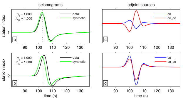
Figure 9: Experiment IIC: data and synthetics. (a–b) Displacement records in the target (black) and in the initial model (green). In the latter case an incorrect source model had the same source-time function but a shifted origin time. Cross-correlation traveltimes $\Delta t_{1}=-0.42$ s and $\Delta t_{2}=-1.50$ s. Double-difference measurements $\Delta\Delta t_{12}=1.08$ s. (c–d) Adjoint sources for the conventional (blue) and for the double-difference cross-correlation (red).

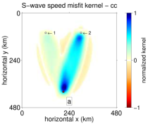
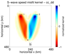
Figure 10: Experiment IIC: misfit sensitivity kernels. (a) Conventional kernel $K_{\beta}(\mathbf{x})$ and (b) double-difference kernel $K_{\beta}^{\tiny\mathrm{dd}}(\mathbf{x})$ from the adjoint sources in Fig. 9c–d. The kernels are very different from one another, with (a) differing greatly from the one in Fig. 6a, but (b) being almost identical to the one in Fig. 6b.

5.2 Realistic phase speed input models, global networks

To test realistic length scales in a global tomography model, we use the global phase velocity map of Trampert & Woodhouse (1995) at periods between 40 s and 150 s, which we mapped to a simplified, unrealistic geometry of a plane with absorbing boundaries. In Experiment IV we model membrane surface waves in this model, as shown in Fig. 13a. The 32 selected earthquakes are shown by red stars, and white circles depict 293 station locations from the global networks.

We use the SPECFEM2D code to model the wavefield. We use 40 elements in latitude and 80 elements in longitude with an average of 4.5^∘ in element size in each direction. The rescaling corresponds to dimensions of one meter per latitudinal degree (^∘) of the original. The source wavelet is a Ricker function with 260 Hz dominant frequency, which should be able to resolve structure down to a scale length of approximately 6.6^∘. The sampling rate is 26 $\mu$s and the recording length 125 ms.

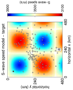
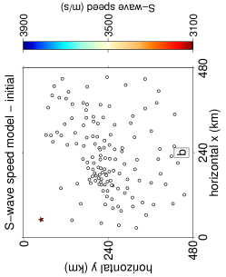
Figure 11: Experiment III: model configuration. One source (star) is placed near the top left corner and 132 stations (circles) are scattered about, off to the lower-right corner of the model space. (a) Target wavespeed model. (b) Initial model.

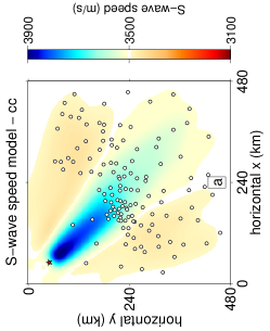
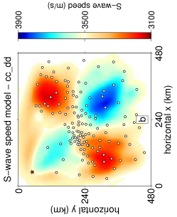
Figure 12: Experiment III: inversion results. Estimated shear-wave speed models with exact source-time function but different origin time. (a) Using conventional cross-correlation traveltime measurements (10 iterations). (b) Using double-difference cross-correlation traveltime measurements (7 iterations).

The initial model is homogeneous with a phase speed of 4500 m/s. Using single-station cross-correlation traveltime measurements, the inversion yields a model that has very limited resolution, shown in Fig. 13b. From double-difference cross-correlation measurements between stations, the inversion reveals structural variations with much greater detail, as shown in Fig. 13c. The conventional tomographic method appears to over-emphasize source-rich areas, which is a result of the summation of all sensitivities along the ray paths emitted from the common source, while obscuring areas with a low density of overlapping ray paths. On the other hand, the double-difference approach, by joining all possible pairs of measurements, does cancel out much of the shared sensitivity and, instead, illuminates wavespeed structure locally among station clusters. With a more realistic geometry on the sphere, we would expect to recover structure in the polar regions and at longitude $180^{\circ}$, as well as gain slight improvements for the interior structure.

5.3 Realistic phase speed input models, regional seismic arrays

Perhaps the greatest contribution of the double-difference tomographic technique as we developed it here will lie in its application to regional seismic arrays. The pairwise combination of seismic measurements should enable imaging local structures with high spatial resolution.

In Experiment V we continue the test of the synthetic model used in the global-scale Experiment IV, but this time with station located at the sites of the Transportable Array (TA) system in the United States. A view of the target model with the source-station geometry marked is shown in Fig. 14a. The average station spacing is about 0.7^∘. The double-difference technique is expected to resolve scale lengths comparable to the station spacing, which is much smaller than the scale of structural variations in this model. We randomly selected 300 stations from the USArray station pool for tomographic testing using membrane surface waves as in all prior experiments.

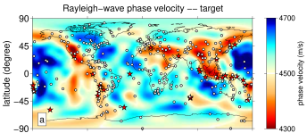
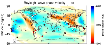
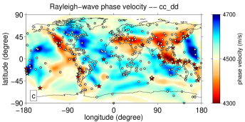
Figure 13: Experiment IV: model and inversion results. (a) The two-dimensional target model, inspired by Trampert & Woodhouse (1995). The stars are 32 earthquakes. The open circles represent 293 global network stations. The initial model is homogeneous. (b) Result after inversion with the conventional cross-correlation traveltime adjoint method (16 iterations). (d) Inversion result from the double-difference cross-correlation traveltime adjoint method (13 iterations).

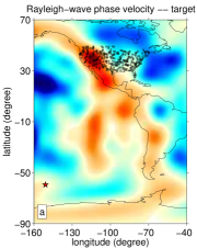
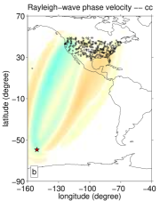
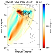
Figure 14: Experiment V: model and inversion results. (a) The two-dimensional target model, a portion of the model shown in Fig. 13a. The star is the single earthquake source used in this study. The open circles represent 300 stations from the USArray network. (b) Inversion result with the conventional cross-correlation traveltime adjoint method (6 iterations). (d) Inversion result using the double-difference method (6 iterations).

The initial model is homogeneous. The inversion result in Fig. 14b was obtained from the adjoint tomography with conventional cross-correlation traveltime measurements recorded at all stations. The model resolves little more than the average wavespeed structure along the common ray path between the earthquake and the array. In contrast, the double-difference method reveals substantial details of the local structure beneath the array, and the perturbations along the direct path are also reasonable. The intrinsic sensitivity of differential measurements will make the double-difference technique ideal for the high-resolution investigation of well-instrumented areas with limited natural seismic activity, or where destructive sources are not an option.

6 C O N C L U S I O N S

In conventional traveltime tomography, source uncertainties and systematic errors introduce artifacts or bias into the estimated wavespeed structure. In the double-difference approach, measurements made on pairs of stations that share a similar source and similar systematic effects are differenced to partially cancel out such consequences. Both theoretically and in numerical experiments, we have shown that the ‘double-difference’ approach produces reliable misfit kernels for adjoint tomography, despite potentially incorrect source wavelets, scale factors, or timings used in synthetic modeling.

Furthermore, double-difference adjoint tomography is an efficient technique to resolve local structure with high resolution. By pairing seismograms from distinct stations with a common source, the technique yields sharp images in the area local to the stations. Those areas are often plagued by smearing artifacts in conventional tomography, especially when limited numbers of earthquakes are available nearby. This opens a wide range of promising applications in seismic array analysis, and especially in areas where the use of active sources is restricted. Fine-scale structure within the array area can be resolved even from a single earthquake.

The double-difference algorithm can be simply implemented into a conventional adjoint tomography scheme, by pairing up all regular measurements. The adjoint sources necessary for the numerical gradient calculations are obtained by summing up contributions from all pairs, which are simultaneously back-propagated to calculate the differential misfit kernels using just one adjoint simulation per iteration.

7 A c k n o w l e d g e m e n t s

YOY expresses her thanks to Min Chen, Paula Koelemeijer, Guust Nolet, and Youyi Ruan for discussions. This research was partially supported by NSF grants EAR-1150145 to FJS and EAR-1112906 to JT, and by a Charlotte Elizabeth Procter Fellowship from Princeton University to YOY. We thank Carl Tape and Vala Hjörleifsdóttir for sharing unpublished notes related to their published work which we cite. The Associate Editor, Jean Virieux, Carl Tape, and one other, anonymous, reviewer are thanked for their thoughtful and constructive comments, which improved our manuscript. Our computer codes are available from https://github.com/yanhuay/seisDD.

8 A P P E N D I X:   D O U B L E - D I F F E R E N C E   M U L T I T A P E R   M E A S U R E M E N T S

In the main text we focused on measuring traveltime shifts via cross-correlation, a time-domain method that does not offer frequency resolution beyond what can be achieved using explicit filtering operations prior to analysis. Such an approach is implicitly justified for the inversion of body waves, but for strongly dispersive waves such as surface waves, we recommend making frequency-dependent measurements of phase and amplitude using the multitaper method Park et al. (1987); Laske & Masters (1996); Zhou et al. (2004); Tape et al. (2009). In this section we discuss its application to the double-difference framework. Our derivations borrow heavily from Hjörleifsdóttir (2007). They are purposely ‘conceptual’ for transparency, and to remain sufficiently flexible for a variety of practical implementation strategies.

8.1 Multitaper measurements of differential phase and amplitude

For notational convenience we distinguish time-domain functions such as $s(t)$ or $d(t)$ from their frequency-domain counterparts $s(\omega)$ and $d(\omega)$ only through their arguments $t$ for time, and $\omega$ for angular frequency. For two stations $i$ and $j$ (always subscripted and thus never to be confused with the imaginary number $i=\sqrt{-1}$), the Fourier-transformed waveforms are assumed to be of the form (e.g., Dziewoński & Hales, 1972; Kennett, 2002)

$$s_{i}(\omega) =A_{i}^{\mathrm{syn}}(\omega)\,e^{-i\omega\,t_{i}^{\mathrm{syn}}(\omega)}\qquad\mbox{and}\qquad s_{j}(\omega)=A_{j}^{\mathrm{syn}}(\omega)\,e^{-i\omega\,t_{j}^{\mathrm{syn}}(\omega)},$$ (25a)

$$d_{i}(\omega) =A_{i}^{\mathrm{obs}}(\omega)\,e^{-i\omega\,t_{i}^{\mathrm{obs}}(\omega)}\qquad\mbox{and}\qquad d_{j}(\omega)=A_{j}^{\mathrm{obs}}(\omega)\,e^{-i\omega\,t_{j}^{\mathrm{obs}}(\omega)}.$$ (25b)

We define the differential frequency-dependent ‘phase’ (compare with eqs 6) and ‘logarithmic amplitude’ anomalies as

$$\Delta t_{ij}^{\mathrm{syn}}(\omega) =t_{i}^{\mathrm{syn}}(\omega)-t_{j}^{\mathrm{syn}}(\omega)\qquad\mbox{and}\qquad\Delta\!\ln\!{A}_{ij}^{\mathrm{syn}}(\omega)=\ln\left[\frac{A_{i}^{\mathrm{syn}}(\omega)}{A_{j}^{\mathrm{syn}}(\omega)}\right],$$ (26a)

$$\Delta t_{ij}^{\mathrm{obs}}(\omega) =t_{i}^{\mathrm{obs}}(\omega)-t_{j}^{\mathrm{obs}}(\omega)\qquad\mbox{and}\qquad\Delta\!\ln\!{A}_{ij}^{\mathrm{obs}}(\omega)=\ln\left[\frac{A_{i}^{\mathrm{obs}}(\omega)}{A_{j}^{\mathrm{obs}}(\omega)}\right].$$ (26b)

We adopt the idealized viewpoint that a trace recorded at a station $i$ may be mapped onto one made at a station $j$ (perhaps after specific phase-windowing, see Maggi et al., 2009, and/or after time-shifting and scaling by a prior all-frequency cross-correlation measurement) via a ‘frequency-response’ or ‘transfer’ function, $\mathcal{T}_{ij}(\omega)$,

$$s_{i}(\omega) =\mathcal{T}_{ij}^{\mathrm{syn}}(\omega)\,s_{j}(\omega),$$ (27a)

$$d_{i}(\omega) =\mathcal{T}_{ij}^{\mathrm{obs}}(\omega)\,d_{j}(\omega).$$ (27b)

Combining eqs (25)–(27), we can rewrite the theoretical ‘transfer functions’ of our model as

$$\mathcal{T}_{ij}^{\mathrm{syn}}(\omega) =e^{\Delta\!\ln\!{A}_{ij}^{\mathrm{syn}}(\omega)-i\omega\Delta t_{ij}^{\mathrm{syn}}(\omega)},$$ (28a)

$$\mathcal{T}_{ij}^{\mathrm{obs}}(\omega) =e^{\Delta\!\ln\!{A}_{ij}^{\mathrm{obs}}(\omega)-i\omega\Delta t_{ij}^{\mathrm{obs}}(\omega)}.$$ (28b)

We have hereby defined $\Delta t_{ij}^{\mathrm{syn}}(\omega)$ and $\Delta t_{ij}^{\mathrm{obs}}(\omega)$ as the frequency-dependent phase differences between $s_{i}(t)$ and $s_{j}(t)$, and $d_{i}(t)$ and $d_{j}(t)$ respectively, and $\Delta\!\ln\!{A}_{ij}^{\mathrm{syn}}(\omega)$ and $\Delta\!\ln\!{A}_{ij}^{\mathrm{obs}}(\omega)$ with their frequency-dependent amplitude differences.

The linear time-invariant model (27) is far from perfect (for a time-and-frequency dependent viewpoint, see, e.g., Kulesh et al., 2005; Holschneider et al., 2005): the transfer functions must be ‘estimated’. Following Laske & Masters (1996), we begin by multiplying each of the individual time-domain records $s_{i}(t)$ and $d_{i}(t)$ by one of a small set of $K$ orthogonal data windows denoted $h^{T\Omega}_{k}(t)$ (here, the prolate spheroidal functions of Slepian, 1978), designed for a particular record length $T$ and for a desired resolution angular-frequency half-bandwidth $\Omega$ Mullis & Scharf (1991); Simons & Plattner (2015), and Fourier-transforming the result to yield the sets

$$s_{i}^{k}(\omega),s_{j}^{k}(\omega)\qquad\mbox{and}\qquad d_{i}^{k}(\omega),d_{j}^{k}(\omega)\quad\mbox{where}\quad k=1,\ldots,\left\lfloor\frac{T\Omega}{\pi}\right\rfloor-1.$$ (29)

At frequencies separated by about $2\Omega$, any differently ‘tapered’ pairs $s^{k},s^{l}$ or $d^{k},d^{l}$ will be almost perfectly uncorrelated statistically Percival & Walden (1993). Using all of them, the transfer function in eq. (28a) can be estimated in the least-squares sense (Bendat & Piersol, 2000, Ch. 9) as minimizing the linear-mapping ‘noise’ power associated with eq. (27a),

$$T_{ij}^{\mathrm{syn}}(\omega)=\frac{\sum_{k}^{K}s_{i}^{k}(\omega)\big{[}s^{k}_{j}(\omega)\big{]}^{*}}{\sum_{k}^{K}s^{k}_{j}(\omega)\big{[}s^{k}_{j}(\omega)\big{]}^{*}}=\operatorname*{\arg\!\min}_{\mathcal{T}_{ij}^{\mathrm{syn}}}\sum_{k}^{K}\left\{s_{i}^{k}(\omega)-\mathcal{T}_{ij}^{\mathrm{syn}}(\omega)s^{k}_{j}(\omega)\right\}^{2}.$$ (30)

The superscripted asterisk (^∗) denotes complex conjugation. We note here for completeness that the associated ‘coherence’ estimate is

$$\gamma^{2}_{ij}(\omega)=\frac{\left|\sum_{k}^{K}s_{i}^{k}(\omega)\big{[}s^{k}_{j}(\omega)\big{]}^{*}\right|^{2}}{\sum_{k}^{K}s^{k}_{i}(\omega)\big{[}s^{k}_{i}(\omega)\big{]}^{*}\sum_{l}^{K}s^{l}_{j}(\omega)\big{[}s^{l}_{j}(\omega)\big{]}^{*}}.$$ (31)

Switching to polar coordinates we write the estimate of the transfer function in terms of its ‘gain factor’ and ‘phase angle’ contributions,

$$T_{ij}^{\mathrm{syn}}(\omega)=\big{|}T_{ij}^{\mathrm{syn}}(\omega)\big{|}e^{-i\phi_{ij}^{\mathrm{syn}}(\omega)},$$ (32)

where

$$\big{|}T_{ij}^{\mathrm{syn}}(\omega)\big{|}=\left(\big{\{}\operatorname{Im}\big{[}T_{ij}^{\mathrm{syn}}(\omega)\big{]}\big{\}}^{2}+\big{\{}\operatorname{Re}\big{[}T_{ij}^{\mathrm{syn}}(\omega)\big{]}\big{\}}^{2}\right)^{1/2}\qquad\mbox{and}\qquad\phi_{ij}^{\mathrm{syn}}(\omega)=-\mbox{atan}\left\{\frac{\operatorname{Im}\big{[}T_{ij}^{\mathrm{syn}}(\omega)\big{]}}{\operatorname{Re}\big{[}T_{ij}^{\mathrm{syn}}(\omega)\big{]}}\right\}.$$ (33)

Uncertainties on the phase angle, gain factor, and coherence estimates are approximately Bendat & Piersol (2000); Simons et al. (2003)

$$\mbox{var}\{\phi_{ij}^{\mathrm{syn}}(\omega)\}\approx\frac{1-\gamma^{2}_{ij}(\omega)}{2K\hskip 1.00006pt\gamma^{2}_{ij}(\omega)},\qquad\mbox{var}\big{\{}|T_{ij}^{\mathrm{syn}}|\big{\}}\approx\frac{1-\gamma^{2}_{ij}(\omega)}{2K\hskip 1.00006pt\gamma^{2}_{ij}(\omega)}\big{|}T_{ij}^{\mathrm{syn}}\big{|}^{2}\qquad\mbox{and}\qquad\mbox{var}\big{\{}\gamma^{2}_{ij}(\omega)\}\approx\frac{\big{[}1-\gamma^{2}_{ij}(\omega)\big{]}^{2}}{K/2}\gamma^{2}_{ij}(\omega),$$ (34)

where we have silently subscribed to the established practice of confusing the estimated (on the left hand side of the expressions) from the ‘true’ quantities (on the right). Alternative estimates of the quantities in eqs (30) and (31) could be obtained through ‘jackknifing’ Chave et al. (1987); Thomson & Chave (1991). We follow Laske & Masters (1996) in using eq. (30) to estimate the transfer function, but we do estimate its variance through the jackknife, which will be conservative Efron & Stein (1981). More detailed distributional considerations are provided by Carter (1987). The utility of eq. (34) lies in the interpretation that highly ‘coherent’ (in the sense of eq. 31) waveforms estimated from a relatively large number of multitapered Fourier-domain ‘projections’ will be, quite generally, very precise.

Through eqs. (28a) and (32), finally, we arrive at our estimates for the frequency-dependent differential phase and amplitude measurements on the synthetic time-series $s_{i}(t)$ and $s_{j}(t)$, namely

$$\Delta t^{\mathrm{syn}}_{ij}(\omega) =\phi_{ij}^{\mathrm{syn}}(\omega)/\omega\qquad\mbox{and}\qquad\Delta\!\ln\!{A}_{ij}^{\mathrm{syn}}(\omega)=\ln\big{|}{T_{ij}^{\mathrm{syn}}(\omega)}\big{|}.$$ (35a)

Exchanging the synthetic time-series for the observed ones in the above expressions, $$s\leftrightarrow d \mathrm{syn}\leftrightarrow\mathrm{obs}$$, accomplishes the desired switch in the superscripted , whence

$$\Delta t^{\mathrm{obs}}_{ij}(\omega) =\phi_{ij}^{\mathrm{obs}}(\omega)/\omega\qquad\mbox{and}\qquad\Delta\!\ln\!{A}_{ij}^{\mathrm{obs}}(\omega)=\ln\big{|}{T_{ij}^{\mathrm{obs}}(\omega)}\big{|}.$$ (35b)

Error propagation will turn eqs (34) into the relevant uncertainties on the differential phase and amplitude measurements in eqs (35).

The logarithmic amplitude measurements in eqs (35) are not skew-symmetric under a change of the station indices, since eq. (30), the estimated transfer function from station $i$ to $j$, is not simply the inverse of the transfer function from station $j$ to $i$, as indeed it need not be: the modeling imperfection in mapping the seismograms is not simply invertible. Instead we find from eqs (30)–(31) that $T_{ij}T_{ji}=\gamma^{2}_{ij}$, suggesting that the required symmetry prevails only at frequencies at which the waveforms are highly coherent. A transfer-function estimate alternative to eq. (30) might thus be $T_{ij}/|\gamma_{ij}|$, as under this scenario a switch in the indices would indeed lead to $\Delta\!\ln\!{A}_{ji}$ being equal to $-\Delta\!\ln\!{A}_{ij}$ under all circumstances of mutual coherency. In the least-squares interpretation we would then be minimizing the ‘noise’ power after mapping one seismogram onto another subject to weighting by the absolute coherence to avoid mapping frequency components at which the signals are incoherent. We do not make this choice (or indeed, any other of many possible options listed by, e.g., Knapp & Carter, 1976) here, but we will revisit the issue of symmetry later in this Appendix.

If the seismogram pairs had been pre-aligned and pre-scaled using conventional cross-correlation, perhaps to improve the stability of the frequency-dependent phase and amplitude expressions (33), these time-domain, frequency-independent, measurements would need to be added to the traveltime and amplitude expressions (35). If specific time windows of interest were being involved, all of the subsequent formalism would continue to hold but, naturally, the effective number of measurement pairs would increase proportionally. And of course, the double-difference multitaper method could follow any number of prior inversions designed to bring the starting model closer to the target; in this context we mention our own work on wavelet multiscale waveform-difference, envelope-difference and envelope-cross-correlation adjoint techniques Yuan & Simons (2014); Yuan et al. (2015).

8.2 Double-difference multitaper measurements, misfit functions, and their gradients

Making differential measurements between stations resolves the intrinsic ambiguity in the attribution of the phase and amplitude behavior of individual seismic records to source-related, structure-induced or instrumental factors Kennett (2002), and for this reason has been the classical approach for many decades Dziewoński et al. (1969); Dziewoński & Hales (1972). But rather than using the differential measurements for the interrogation of subsurface structure on the interstation portion of the great circle connecting one source to one pair of receivers, we now proceed to making, and using, differential measurements between all pairs of stations into a tool for adjoint tomography. We take our cue from eq. (7) and use eqs (35) to define the ‘double-difference’ frequency-dependent traveltime and amplitude measurements made between stations $i$ and $j$, namely

$$\Delta\Delta t_{ij}(\omega) =\Delta t_{ij}^{\mathrm{syn}}(\omega)-\Delta t_{ij}^{\mathrm{obs}}(\omega)\qquad\mbox{and}\qquad\Delta\Delta\!\ln\!{A}_{ij}(\omega)=\Delta\!\ln\!{A}_{ij}^{\mathrm{syn}}(\omega)-\Delta\!\ln\!{A}_{ij}^{\mathrm{obs}}(\omega).$$ (36a)

As in eq. (8), we incorporate those into a phase and an amplitude misfit function defined over the entire available bandwidth and for all station pairs, i.e.

$$\chi_{\Phi}^{\tiny\mathrm{dd}} =\frac{1}{2}\sum_{i}\sum_{j>i}\sum_{\omega}W_{\Phi}(\omega)\big{[}\Delta\Delta t_{ij}(\omega)\big{]}^{2},$$ (37a)

$$\chi_{A}^{\tiny\mathrm{dd}} =\frac{1}{2}\sum_{i}\sum_{j>i}\sum_{\omega}W_{A}(\omega)\big{[}\Delta\Delta\!\ln\!{A}_{ij}(\omega)\big{]}^{2},$$ (37b)

with $W_{\Phi}(\omega)$ and $W_{A}(\omega)$ appropriate weight functions. The weighted sum over all frequencies is meant to be respectful of the effective bandwidth of the estimates derived via eq. (30) from seismic records $s_{i}(t)$, $s_{j}(t)$ and $d_{i}(t)$, $d_{j}(t)$ multitapered by the Slepian window set $h^{T\Omega}_{k}(t)$, $k=1,\ldots,\left\lfloor T\Omega/\pi\right\rfloor-1$. The multitaper procedure implies ‘tiling’ the frequency axis over the entire bandwidth in pieces of phase and amplitude ‘information’ extracted over time portions of length $T$, centered on individual frequencies $\omega$, that are approximately uncorrelated when spaced $2\Omega$ apart Walden (1990); Walden et al. (1995). The simplest form of the weight function is thus $W_{\Phi}(\omega)=W_{A}(\omega)=2\Omega$, for a discrete set of angular frequencies $\omega=\Omega,3\Omega,\ldots$ until the complete signal bandwidth is exhausted, tapering slightly at the edges of the frequency axis to smoothly contain the full bandwidth of the seismograms. Alternatively, to serve the purpose of filtering out frequencies containing incoherent energy (Bendat & Piersol, 2000, Ch. 6), $W_{\Phi}(\omega)$ and $W_{A}(\omega)$ can be the inverse of the phase and amplitude variances (34), and, if subsampling is undesirable, they should reflect the inverse full covariances of the estimates between frequencies Percival & Walden (1993).

As in eq. (9), the derivatives of the differential objective functions in eqs (37) are

$$\delta\chi_{\Phi}^{\tiny\mathrm{dd}} =\sum_{i}\sum_{j>i}\sum_{\omega}W_{\Phi}(\omega)[\Delta\Delta t_{ij}(\omega)]\,\delta\Delta t^{\mathrm{syn}}_{ij}(\omega),$$ (38a)

$$\delta\chi_{A}^{\tiny\mathrm{dd}} =\sum_{i}\sum_{j>i}\sum_{\omega}W_{A}(\omega)[\Delta\Delta\!\ln\!{A}_{ij}(\omega)]\,\delta\Delta\!\ln\!{A}^{\mathrm{syn}}_{ij}(\omega),$$ (38b)

where $\delta\Delta t^{\mathrm{syn}}_{ij}(\omega)$ is the perturbation of the frequency-dependent differential traveltime $\Delta t_{ij}^{\mathrm{syn}}(\omega)$ due to a model perturbation, and $\delta\Delta\!\ln\!{A}^{\mathrm{syn}}_{ij}(\omega)$ the perturbation of the frequency-dependent differential amplitude $\Delta\!\ln\!{A}_{ij}^{\mathrm{syn}}(\omega)$. It is for the terms $\delta\Delta t^{\mathrm{syn}}_{ij}(\omega)$ and $\delta\Delta\!\ln\!{A}^{\mathrm{syn}}_{ij}(\omega)$ that we will construct expressions leading to a new set of adjoint sources.

8.3 Double-difference multitaper adjoint sources

By taking perturbations to the formula in (28a) in its estimated (italicized) form, we have

$$\delta T_{ij}^{\mathrm{syn}}(\omega) =T_{ij}^{\mathrm{syn}}(\omega)\big{[}\delta\Delta\!\ln\!{A}^{\mathrm{syn}}_{ij}(\omega)-i\omega\delta\Delta t^{\mathrm{syn}}_{ij}(\omega)\big{]}.$$ (39)

Dropping the argument that captures the dependence on frequency for notational convenience, we use the product and chain rules for differentiation to write the total derivative of eq. (30) as

$$\delta T_{ij}^{\mathrm{syn}} =\frac{1}{S_{jj}}\sum_{k}^{K}\,[s_{j}^{k}]^{*}\,\delta s_{i}^{k}-T_{ij}^{\mathrm{syn}}[s_{j}^{k}]^{*}\,\delta s_{j}^{k}+\left(s_{i}^{k}-T_{ij}^{\mathrm{syn}}s_{j}^{k}\right)\,\delta[s_{j}^{k}]^{*}.$$ (40)

We introduced a symbol for the multitapered (cross-) power-spectral density estimates

$$S_{ij}=\sum_{k}^{K}s^{k}_{i}[s^{k}_{j}]^{*}\quad\mbox{with}\quad T_{ij}^{\mathrm{syn}}=\frac{\displaystyle{S_{ij}}}{\displaystyle{S_{jj}}}\qquad\mbox{and}\qquad S_{ij}^{*}=S_{ji},$$ (41)

which of course upholds the relation eq. (30). Combining eqs. (39)–(40) and using eq (30) again, we then obtain the perturbations

$$\delta\Delta t^{\mathrm{syn}}_{ij}(\omega) =\frac{i}{2\omega}\sum_{k}^{K}\frac{[s_{j}^{k}]^{*}}{S_{ij}}\,\delta s_{i}^{k}-\frac{s_{j}^{k}}{S_{ij}^{*}}\,\delta[s_{i}^{k}]^{*}-\frac{[s_{i}^{k}]^{*}}{S_{ij}^{*}}\,\delta s_{j}^{k}+\frac{s_{i}^{k}}{S_{ij}}\,\delta[s_{j}^{k}]^{*}$$ (42)

through straightforward manipulation, and, likewise,

$$\delta\Delta\!\ln\!{A}^{\mathrm{syn}}_{ij}(\omega) =\frac{1}{2}\sum_{k}^{K}\frac{[s_{j}^{k}]^{*}}{S_{ij}}\,\delta s_{i}^{k}+\frac{s_{j}^{k}}{S_{ij}^{*}}\,\delta[s_{i}^{k}]^{*}+\left(\frac{[s_{i}^{k}]^{*}}{S_{ij}^{*}}-2\frac{[s_{j}^{k}]^{*}}{S_{jj}}\right)\delta s_{j}^{k}+\left(\frac{s_{i}^{k}}{S_{ij}}-2\frac{s_{j}^{k}}{S_{jj}}\right)\delta[s_{j}^{k}]^{*}.$$ (43)

We shall associate the frequency-dependent partials that appear in eqs (42)–(43) with the symbols

$$p_{i|j}^{k}(\omega) =\frac{i}{2\omega}\frac{[s_{j}^{k}]^{*}}{S_{ij}}\qquad\mbox{and}\qquad p_{j|i}^{k}(\omega)=\frac{-i}{2\omega}\frac{[s_{i}^{k}]^{*}}{S_{ij}^{*}},$$ (44a)

$$a_{i|j}^{k}(\omega) =\frac{1}{2}\frac{[s_{j}^{k}]^{*}}{S_{ij}}\qquad\mbox{and}\qquad a_{j|i}^{k}(\omega)=\frac{1}{2}\frac{[s_{i}^{k}]^{*}}{S_{ij}^{*}}-\frac{[s_{j}^{k}]^{*}}{S_{jj}},$$ (44b)

and their conjugates. Again, we remark on the lack of station symmetry in the amplitude terms (44b). However, it is noteworthy that, via the Fourier identity $\partial_{t}\leftrightarrow i\omega$, the terms in the expressions (44a) are identical (up to the sign) to the (first) terms in eq. (44b) if in the latter, the time-domain seismograms are substituted for their time-derivatives. Consequently, we may recognize eqs (42)–(43) as the (differential) frequency-dependent (narrow-band) multitaper generalization of the traveltime expressions (3) and (15), familiar from Dahlen et al. (2000), and of their amplitude-anomaly counterparts, see Dahlen & Baig (2002). With these conventions in place, the derivatives of the multitaper objective functions in eq. (38) are now given by

$$\delta\chi^{\tiny\mathrm{dd}}_{\Phi}= \sum_{i}\sum_{j>i}\sum_{k}^{K}\sum_{\omega}W_{\Phi}(\omega)[\Delta\Delta t_{ij}(\omega)]\left\{p_{i|j}^{k}(\omega)\,\delta s_{i}^{k}(\omega)+[p_{i|j}^{k}(\omega)]^{*}\,\delta[s_{i}^{k}(\omega)]^{*}+p_{j|i}^{k}(\omega)\,\delta s_{j}^{k}(\omega)+[p_{j|i}^{k}(\omega)]^{*}\,\delta[s_{j}^{k}(\omega)]^{*}\right\},$$ (45a)

$$\delta\chi^{\tiny\mathrm{dd}}_{A}= \sum_{i}\sum_{j>i}\sum_{k}^{K}\sum_{\omega}W_{A}(\omega)[\Delta\Delta\!\ln\!{A}_{ij}(\omega)]\left\{a_{i|j}^{k}(\omega)\,\delta s_{i}^{k}(\omega)+[a_{i|j}^{k}(\omega)]^{*}\,\delta[s_{i}^{k}(\omega)]^{*}+a_{j|i}^{k}(\omega)\,\delta s_{j}^{k}(\omega)+[a_{j|i}^{k}(\omega)]^{*}\,\delta[s_{j}^{k}(\omega)]^{*}\right\}.$$ (45b)

We introduce the time-domain functions, inverse-Fourier transformed from their frequency-domain product counterparts,

$$\mathscr{S}_{i|j}(t) =\sum_{k}^{K}h^{T\Omega}_{k}(t)\,\mathcal{F}^{-1}\!\left\{W_{\Phi}[\Delta\Delta t_{ij}]\,p_{i|j}^{k}\right\}\!(t),\qquad\mbox{and}\qquad\mathscr{S}_{j|i}(t)=\sum_{k}^{K}h^{T\Omega}_{k}(t)\,\mathcal{F}^{-1}\!\left\{W_{\Phi}[\Delta\Delta t_{ij}]\,p_{j|i}^{k}\right\}\!(t),$$ (46a)

$$\mathscr{A}_{i|j}(t) =\sum_{k}^{K}h^{T\Omega}_{k}(t)\,\mathcal{F}^{-1}\!\left\{W_{A}[\Delta\Delta\!\ln\!{A}_{ij}]\,a_{i|j}^{k}\right\}\!(t)\qquad\mbox{and}\qquad\mathscr{A}_{j|i}(t)=\sum_{k}^{K}h^{T\Omega}_{k}(t)\,\mathcal{F}^{-1}\!\left\{W_{A}[\Delta\Delta\!\ln\!{A}_{ij}]\,a_{j|i}^{k}\right\}\!(t),$$ (46b)

with which we are able to rewrite eqs (45) in the time domain, via Plancherel’s relation as applicable over the record section of length $T$. We have simultaneously extricated the tapers from their seismograms, $\delta s_{i}^{k}(t)=\delta[s_{i}^{k}(t)]^{*}=h^{T\Omega}_{k}(t)\,\delta s_{i}(t)$, and used the real-valuedness of the time-series to arrive at the recognizable (see eq. 17) form

$$\delta\chi^{\tiny\mathrm{dd}}_{\Phi}= \int_{0}^{T}\left\{\sum_{i}\left[4\pi\sum_{j>i}\mathscr{S}_{i|j}(t)\right]\delta s_{i}(t)+\sum_{j}\left[4\pi\sum_{i<j}\mathscr{S}_{j|i}(t)\right]\delta s_{j}(t)\right\}\hskip 1.00006pt\mathrm{d}t,$$ (47a)

$$\delta\chi^{\tiny\mathrm{dd}}_{A}= \int_{0}^{T}\left\{\sum_{i}\left[4\pi\sum_{j>i}\mathscr{A}_{i|j}(t)\right]\delta a_{i}(t)+\sum_{j}\left[4\pi\sum_{i<j}\mathscr{A}_{j|i}(t)\right]\delta a_{j}(t)\right\}\hskip 1.00006pt\mathrm{d}t.$$ (47b)

The multitaper phase and amplitude adjoint sources are thus

$$f_{\Phi,i}^{\dagger}(t) =4\pi\sum_{j>i}\mathscr{S}_{i|j}(T-t)\,\delta(\mathbf{x}-\mathbf{x}_{i})\qquad\mbox{and}\qquad f_{\Phi,j}^{\dagger}(t)=4\pi\sum_{i<j}\mathscr{S}_{j|i}(T-t)\,\delta(\mathbf{x}-\mathbf{x}_{j}),$$ (48)

$$f_{A,i}^{\dagger}(t) =4\pi\sum_{j>i}\mathscr{A}_{i|j}(T-t)\,\delta(\mathbf{x}-\mathbf{x}_{i})\qquad\mbox{and}\qquad f_{A,j}^{\dagger}(t)=4\pi\sum_{i<j}\mathscr{A}_{j|i}(T-t)\,\delta(\mathbf{x}-\mathbf{x}_{j}).$$ (49)

It is gratifying to discover that eq. (48) is indeed the multitaper generalization of eqs (18), which themselves generalized eq. (4). For its part, eq. (49), ultimately, is the double-difference multitaper generalization of the amplitude-tomography adjoint source derived by, e.g., Tromp et al. (2005), but which we have not given any further consideration in the main text.

Finally, we return to the issue of symmetry in the differential amplitude estimation, which can be restored by replacing all separate summations of the type $\sum_{i}\sum_{j>i}$ and $\sum_{j}\sum_{i<j}$ that appear in the expressions above by a common $\sum_{ij}$.

With these expressions we are finally able to define the multitaper misfit sensitivity kernels along the same lines as eqs (5) and (19), one for the phase and one for the amplitude measurements, both in terms of the velocity perturbation — we are (yet) not concerned with variations in intrinsic attenuation (e.g., Tian et al., 2009, 2011; Zhu et al., 2013).

8.4 Numerical experiment

Fig. 15a shows a simple two-dimensional vertical S-wave speed model with an anomalous layer that divides the model into three segments: a top portion with an S-wave speed of 800 m/s, a middle with a speed of 1000 m/s, and a bottom with a speed of 800 m/s. The initial model, shown in Fig. 15b, possesses the same tripartite geometry but the wavespeeds have different values: at the top 900 m/s, in the middle 800 m/s, and at the bottom 1000 m/s.

Synthetics were computed used one point-source Ricker wavelet with 40 Hz dominant frequency located at 0.5 m depth, at a horizontal distance of 100 m from the left edge of the model. Two receivers were placed at the surface in the positions shown in Fig. 15.

Fig. 16 shows the observed and synthetic records (a–b), the adjoint sources (c–d), and the double-difference frequency-dependent multitaper phase measurement (e). Fig. 17 compares the misfit sensitivity kernel of the double-difference time-domain cross-correlation measurement to the misfit sensitivity kernel of the double-difference multitaper phase measurement, which shows some additional structure.

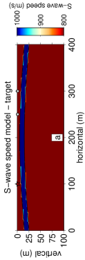
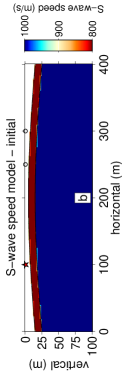
Figure 15: Experiment with multitaper phase and amplitude measurements. (a) Target model. (b) Initial model. The star is the source, the open circles depict two stations.

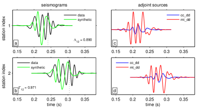
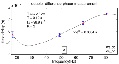
Figure 16: Experiment with multitaper phase and amplitude measurements. (a–b) Data and synthetics. (c–d) Adjoint sources. (e) Double-difference phase measurements. The solid line are the multitaper estimates, with standard errors estimated using jackknifing. The dashed line is the cross-correlation value.

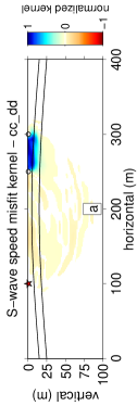
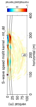
Figure 17: Misfit sensitivity kernel for the (a) double-difference of cross-correlation traveltimes and for the (b) double-difference of multitaper phase measurements. The star is the source, the open circles two stations.

References

- Abers & Roecker (1991) Abers, G. A. & Roecker, S. W., 1991. Deep structure of an arc-continent collision: Earthquake relocation and inversion for upper mantle P and S wave velocities beneath Papua New Guinea, J. Geophys. Res., 96(B4), 6379–6401.
- Baig et al. (2003) Baig, A. M., Dahlen, F. A. & Hung, S.-H., 2003. Traveltimes of waves in three-dimensional random media, Geophys. J. Int., 153(2), 467–482, doi: 10.1046/j.1365–246X.2003.01905.x.
- Bendat & Piersol (2000) Bendat, J. S. & Piersol, A. G., 2000. Random Data: Analysis and Measurement Procedures, John Wiley, New York, 3rd edn.
- Brune & Dorman (1963) Brune, J. & Dorman, J., 1963. Seismic waves and earth structure in the Canadian shield, Bull. Seism. Soc. Am., 53(1), 167–210.
- Burdick et al. (2014) Burdick, S., van der Hilst, R. D., Vernon, F. L., Martynov, V., Cox, T., Eakins, J., Karasu, G. H., Tylell, J., Astiz, L. & Pavlis, G. L., 2014. Model update January 2013: Upper mantle heterogeneity beneath North America from travel-time tomography with global and USArray Transportable Array data, Seismol. Res. Lett., 85(1), 77–81, doi: 10.1785/0220130098.
- Carter (1987) Carter, G. C., 1987. Coherence and time-delay estimation, Proc. IEEE, 75, 236–255.
- Chave et al. (1987) Chave, A. D., Thomson, D. J. & Ander, M. E., 1987. On the robust estimation of power spectra, coherences, and transfer functions, J. Geophys. Res., 92(B1), 633–648.
- Chen et al. (2007) Chen, P., Jordan, T. H. & Zhao, L., 2007. Full three-dimensional tomography: a comparison between the scattering-integral and adjoint-wavefield methods, Geophys. J. Int., 170(1), 175–181, doi: 10.1111/j.1365–246X.2007.03429.x.
- Curtis & Snieder (1997) Curtis, A. & Snieder, R., 1997. Reconditioning inverse problems using the genetic algorithm and revised parameterization, Geophysics, 62(4), 1524–1532.
- Dahlen & Baig (2002) Dahlen, F. A. & Baig, A., 2002. Fréchet kernels for body-wave amplitudes, Geophys. J. Int., 150, 440–466, doi: 10.1046/j.1365–246X.2002.01718.x.
- Dahlen et al. (2000) Dahlen, F. A., Hung, S.-H. & Nolet, G., 2000. Fréchet kernels for finite-frequency traveltimes — I. Theory, Geophys. J. Int., 141(1), 157–174, doi: 10.1046/j.1365–246X.2000.00070.x.
- de Vos et al. (2013) de Vos, D., Paulssen, H. & Fichtner, A., 2013. Finite-frequency sensitivity kernels for two-station surface wave measurements, Geophys. J. Int., 194(2), 1042–1049, doi: 10.1093/gji/ggt144.
- Dziewoński & Hales (1972) Dziewoński, A. & Hales, A. L., 1972, Numerical analysis of dispersed seismic waves, in Seismology: Surface Waves and Earth Oscillations, edited by B. A. Bolt, B. Alder, S. Fernbach, & M. Rotenberg, vol. 11 of Methods In Computational Physics, pp. 39–84, Academic Press, San Diego, Calif.
- Dziewoński et al. (1969) Dziewoński, A. M., Block, S. & Landisman, M., 1969. A technique for the analysis of transient seismic signals, Bull. Seism. Soc. Am., 59(1), 427–444.
- Efron & Stein (1981) Efron, B. & Stein, C., 1981. The jackknife estimate of variance, Ann. Stat., 9(3), 586–596.
- Fang & Zhang (2014) Fang, H. & Zhang, H., 2014. Wavelet-based double-difference seismic tomography with sparsity regularization, Geophys. J. Int., 199(2), 944–955, doi: 10.1093/gji/ggu305.
- Fichtner & Trampert (2011) Fichtner, A. & Trampert, J., 2011. Resolution analysis in full waveform inversion, Geophys. J. Int., 187(3), 1604–1624, doi: 10.1111/j.1365–246X.2011.05218.x.
- Fichtner et al. (2008) Fichtner, A., Kennett, B. L. N., Igel, H. & Bunge, H.-P., 2008. Theoretical background for continental-and global-scale full-waveform inversion in the time–frequency domain, Geophys. J. Int., 175(2), 665–685, doi: 10.1111/j.1365–246X.2008.03923.x.
- Got et al. (1994) Got, J.-L., Fréchet, J. & Klein, F. W., 1994. Deep fault plane geometry inferred from multiplet relative relocation beneath the south flank of Kilauea, J. Geophys. Res., 99(B8), 15375–15386.
- Hjörleifsdóttir (2007) Hjörleifsdóttir, V., 2007, Earthquake Source Characterization Using 3d Numerical Modeling, Ph.D. thesis, California Institute of Technology, Pasadena, Calif.
- Holschneider et al. (2005) Holschneider, M., Diallo, M. S., Kulesh, M., Ohrnberger, M., Lück, E. & Scherbaum, F., 2005. Characterization of dispersive surface waves using continuous wavelet transforms, Geophys. J. Int., 163(2), 463–478, doi: 10.1111/j.1365–246X.2005.02787.x.
- Hudson & Heritage (1981) Hudson, J. A. & Heritage, J. R., 1981. The use of the Born approximation in seismic scattering problems, Geophys. J. Int., 66(1), 221–240, doi: 10.1111/j.1365–246X.1981.tb05954.x.
- Hung et al. (2000) Hung, S.-H., Dahlen, F. A. & Nolet, G., 2000. Fréchet kernels for finite-frequency traveltimes — II. Examples, Geophys. J. Int., 141(1), 175–203, doi: 10.1046/j.1365–246X.2000.00072.x.
- Hung et al. (2004) Hung, S.-H., Shen, Y. & Chiao, L.-Y., 2004. Imaging seismic velocity structure beneath the Iceland hot spot: A finite frequency approach, J. Geophys. Res., 109(B8), B08305, doi: 10.1029/2003JB002889.
- Kennett (2002) Kennett, B. L. N., 2002. The Seismic Wavefield, vol. II: Interpretation of Seismograms on Regional and Global Scales, Cambridge Univ. Press, Cambridge, UK.
- Knapp & Carter (1976) Knapp, C. H. & Carter, G. C., 1976. The generalized correlation method for estimation of time delay, IEEE Trans. Acoust. Speech Signal Process., 24(4), 320–327, doi: 10.1109/TASSP.1976.1162830.
- Komatitsch & Tromp (2002a) Komatitsch, D. & Tromp, J., 2002a. Spectral-element simulations of global seismic wave propagation — I. Validation, Geophys. J. Int., 149(2), 390–412, doi: 10.1046/j.1365–246X.2002.01653.x.
- Komatitsch & Tromp (2002b) Komatitsch, D. & Tromp, J., 2002b. Spectral-element simulations of global seismic wave propagation — II. Three-dimensional models, oceans, rotation and self-gravitation, Geophys. J. Int., 150(1), 303–318, doi: 10.1046/j.1365–246X.2002.01716.x.
- Komatitsch & Vilotte (1998) Komatitsch, D. & Vilotte, J. P., 1998. The spectral element method: An efficient tool to simulate the seismic response of 2D and 3D geological structures, Bull. Seism. Soc. Am., 88(2), 368–392.
- Kulesh et al. (2005) Kulesh, M., Holschneider, M., Diallo, M. S., Xie, Q., & Scherbaum, F., 2005. Modeling of wave dispersion using continuous wavelet transforms, Pure Appl. Geophys., 162, 843–855, doi: 10.1007/s00024–004–2644–9.
- Laske & Masters (1996) Laske, G. & Masters, G., 1996. Constraints on global phase velocity maps from long-period polarization data, J. Geophys. Res., 101(B7), 16059–16075, doi: 10.1029/96JB00526.
- Liu & Tromp (2006) Liu, Q. & Tromp, J., 2006. Finite-frequency sensitivity kernels based upon adjoint methods, Bull. Seism. Soc. Am., 96(6), 2383–2397, doi: 10.1785/0120060041.
- Luo & Schuster (1991) Luo, Y. & Schuster, G. T., 1991. Wave-equation traveltime inversion, Geophysics, 56(5), 654–663.
- Luo et al. (2015) Luo, Y., Modrak, R. & Tromp, J., 2015, Strategies in adjoint tomography, in Handbook of Geomathematics, edited by W. Freeden, M. Z. Nashed, & T. Sonar, pp. 1943–2001, doi: 10.1007/2F978–3–642–27793–1_96–2, Springer, Heidelberg, Germany, 2nd edn.
- Maggi et al. (2009) Maggi, A., Tape, C., Chen, M., Chao, D. & Tromp, J., 2009. An automated time-window selection algorithm for seismic tomography, Geophys. J. Int., 178(1), 257–281.
- Marquering et al. (1999) Marquering, H., Dahlen, F. A. & Nolet, G., 1999. Three-dimensional sensitivity kernels for finite-frequency travel times: The banana-doughnut paradox, Geophys. J. Int., 137(3), 805–815, doi: 10.1046/j.1365–246x.1999.00837.x.
- Maupin & Kolstrup (2015) Maupin, V. & Kolstrup, M. L., 2015. Insights in P-and S-wave relative traveltime tomography from analysing finite-frequency Fréchet kernels, Geophys. J. Int., 202(3), 1581–1598. doi: 10.1093/gji/ggv239.
- Monteiller et al. (2005) Monteiller, V., Got, J.-L., Virieux, J. & Okubo, P., 2005. An efficient algorithm for double-difference tomography and location in heterogeneous media, with an application to the Kilauea volcano, J. Geophys. Res., 110, B12306, doi:10.1029/2004JB003466.
- Mullis & Scharf (1991) Mullis, C. T. & Scharf, L. L., 1991, Quadratic estimators of the power spectrum, in Advances in Spectrum Analysis and Array Processing, edited by S. Haykin, vol. 1, chap. 1, pp. 1–57, Prentice-Hall, Englewood Cliffs, N. J.
- Nissen-Meyer et al. (2007) Nissen-Meyer, T., Dahlen, F. A. & Fournier, A., 2007. Spherical-earth Fréchet sensitivity kernels, Geophys. J. Int., 168(3), 1051–1066, doi: 10.1111/j.1365–246X.2006.03123.x.
- Nolet (1996) Nolet, G., 1996, A general view on the seismic inverse problem, in Seismic Modelling of Earth Structure, edited by E. Boschi, G. Ekström, & A. Morelli, pp. 1–29, Editrice Compositori,, Bologna, Italy.
- Nolet (2008) Nolet, G., 2008. A Breviary for Seismic Tomography, Cambridge Univ. Press, Cambridge, UK.
- Panning & Romanowicz (2006) Panning, M. & Romanowicz, B., 2006. A three-dimensional radially anisotropic model of shear velocity in the whole mantle, Geophys. J. Int., 167(1), 361–379, doi: 10.1111/j.1365–246X.2006.03100.x.
- Panning et al. (2009) Panning, M. P., Capdeville, Y. & Romanowicz, B. A., 2009. Seismic waveform modelling in a 3-D Earth using the Born approximation: potential shortcomings and a remedy, Geophys. J. Int., 177(1), 161–178, doi: 10.1111/j.1365–246X.2008.04050.x.
- Park et al. (1987) Park, J., Lindberg, C. R. & III, F. L. V., 1987. Multitaper spectral analysis of high-frequency seismograms, J. Geophys. Res., 92(B12), 12675–12684, doi: 10.1029/JB092iB12p12675.
- Passier & Snieder (1995) Passier, M. L. & Snieder, R. K., 1995. Using differential waveform data to retrieve local S velocity structure or path-averaged S velocity gradients, J. Geophys. Res., 100(B12), 24061–24078.
- Pavlis & Booker (1980) Pavlis, G. L. & Booker, J. R., 1980. The mixed discrete-continuous inverse problem: Application to the simultaneous determination of earthquake hypocenters and velocity structure, J. Geophys. Res., 85(B9), 4801–4810, doi: 10.1029/JB085iB09p04801.
- Percival & Walden (1993) Percival, D. B. & Walden, A. T., 1993. Spectral Analysis for Physical Applications, Multitaper and Conventional Univariate Techniques, Cambridge Univ. Press, New York.
- Peter et al. (2007) Peter, D., Tape, C., Boschi, L. & Woodhouse, J. H., 2007. Surface wave tomography: global membrane waves and adjoint methods, Geophys. J. Int., 171(3), 1098–1117, doi: 10.1111/j.1365–246X.2007.03554.x.
- Poupinet et al. (1984) Poupinet, G., Ellsworth, W. L. & Fréchet, J., 1984. Monitoring velocity variations in the crust using earthquake doublets: An application to the Calaveras fault, California, J. Geophys. Res., 89(B7), 5719–5731.
- Rietbrock & Waldhauser (2004) Rietbrock, A. & Waldhauser, F., 2004. A narrowly spaced double-seismic zone in the subducting Nazca plate, Geophys. Res. Lett., 31, L10608, doi: 10.1029/2004GL019610.
- Rost & Thomas (2002) Rost, S. & Thomas, C., 2002. Array seismology: Methods and applications, Rev. Geophys., 40(3), 1008.
- Rubin et al. (1999) Rubin, A. M., Gillard, D. & Got, J.-L., 1999. Streaks of microearthquakes along creeping faults, Nature, 400, 635–641.
- Schaeffer & Lebedev (2013) Schaeffer, A. J. & Lebedev, S., 2013. Global shear speed structure of the upper mantle and transition zone, Geophys. J. Int., 194(1), 441–449, doi: 10.1093/gji/ggt095.
- Schaff & Richards (2004) Schaff, D. P. & Richards, P. G., 2004. Repeating seismic events in China, Science, 303(5661), 1176–1178, doi: 10.1126/science.1093422.
- Simmons et al. (2012) Simmons, N. A., Myers, S. C., Johannesson, G. & Matzel, E., 2012. LLNL-G3Dv3: Global P wave tomography model for improved regional and teleseismic travel time prediction, J. Geophys. Res., 117, B10302, doi: 10.1029/2012JB009525.
- Simons & Plattner (2015) Simons, F. J. & Plattner, A., 2015, Scalar and vector Slepian functions, spherical signal estimation and spectral analysis, in Handbook of Geomathematics, edited by W. Freeden, M. Z. Nashed, & T. Sonar, pp. 2563–2608, doi: 10.1007/978–3–642–54551–1_30, Springer, Heidelberg, Germany, 2nd edn.
- Simons et al. (2003) Simons, F. J., van der Hilst, R. D. & Zuber, M. T., 2003. Spatiospectral localization of isostatic coherence anisotropy in Australia and its relation to seismic anisotropy: Implications for lithospheric deformation, J. Geophys. Res., 108(B5), 2250, doi: 10.1029/2001JB000704.
- Slepian (1978) Slepian, D., 1978. Prolate spheroidal wave functions, Fourier analysis and uncertainty — V: The discrete case, Bell Syst. Tech. J., 57, 1371–1429.
- Spakman & Bijwaard (2001) Spakman, W. & Bijwaard, H., 2001. Optimization of cell parameterization for tomographic inverse problems, Pure Appl. Geophys., 158(8), 1401–1423.
- Spencer & Gubbins (1980) Spencer, C. & Gubbins, D., 1980. Travel-time inversion for simultaneous earthquake location and velocity structure determination in laterally varying media, Geophys. J. R. Astron. Soc., 63(1), 95–116, doi: 10.1111/j.1365–246X.1980.tb02612.x.
- Tanimoto (1990) Tanimoto, T., 1990. Modelling curved surface wave paths: membrane surface wave synthetics, Geophys. J. Int., 102(1), 89–100, doi: 10.1111/j.1365–246X.1990.tb00532.x.
- Tape et al. (2007) Tape, C., Liu, Q. & Tromp, J., 2007. Finite-frequency tomography using adjoint methods — Methodology and examples using membrane surface waves, Geophys. J. Int., 168, 1105–1129, doi: 10.1111/j.1365–246X.2006.03191.x.
- Tape et al. (2009) Tape, C., Liu, Q., Maggi, A. & Tromp, J., 2009. Adjoint tomography of the Southern California crust, Science, 325, 988–992, doi: 10.1126/science.1175298.
- Tarantola (1987) Tarantola, A., 1987, Inversion of travel time and seismic waveforms, in Seismic Tomography, edited by G. Nolet, chap. 6, pp. 135–157, Reidel, Hingham, Mass.
- Tarantola (1988) Tarantola, A., 1988. Theoretical background for the inversion of seismic waveforms, including elasticity and attenuation, Pure Appl. Geophys., 128(1–2), 365–399.
- Thomson & Chave (1991) Thomson, D. J. & Chave, A. D., 1991, Jackknifed error estimates for spectra, coherences, and transfer functions, in Advances in Spectrum Analysis and Array Processing, edited by S. Haykin, vol. 1, chap. 2, pp. 58–113, Prentice-Hall, Englewood Cliffs, N. J.
- Thurber (1992) Thurber, C. H., 1992. Hypocenter-velocity structure coupling in local earthquake tomography, Phys. Earth Planet. Inter., 75(1–3), 55–62, doi:10.1016/0031–9201(92)90117–E.
- Tian et al. (2009) Tian, Y., Sigloch, K. & Nolet, G., 2009. Multiple-frequency SH-wave tomography of the western US upper mantle, Geophys. J. Int., 178(3), 1384–1402, doi: 10.1111/j.1365–246X.2009.04225.x.
- Tian et al. (2011) Tian, Y., Zhou, Y., Sigloch, K., Nolet, G. & Laske, G., 2011. Structure of North American mantle constrained by simultaneous inversion of multiple-frequency SH, SS, and Love waves, J. Geophys. Res., 116, B02307, doi: 10.1029/2010JB007704.
- Trampert & Woodhouse (1995) Trampert, J. & Woodhouse, J. H., 1995. Global phase-velocity maps of Love and Rayleigh-waves between 40 and 150 seconds, Geophys. J. Int., 122(2), 675–690.
- Tromp et al. (2005) Tromp, J., Tape, C. & Liu, Q., 2005. Seismic tomography, adjoint methods, time reversal and banana-doughnut kernels, Geophys. J. Int., 160, 195–216, doi: 10.1111/j.1365–246X.2004.02453.x.
- VanDecar & Crosson (1990) VanDecar, J. C. & Crosson, R. S., 1990. Determination of teleseismic relative phase arrival times using multi-channel cross-correlation and least squares, Bull. Seism. Soc. Am., 80(1), 150–169.
- Walden (1990) Walden, A. T., 1990. Improved low-frequency decay estimation using the multitaper spectral-analysis method, Geophys. Prospect., 38, 61–86.
- Walden et al. (1995) Walden, A. T., McCoy, E. J. & Percival, D. B., 1995. The effective bandwidth of a multitaper spectral estimator, Biometrika, 82(1), 201–214.
- Waldhauser & Ellsworth (2000) Waldhauser, F. & Ellsworth, W. L., 2000. A double-difference earthquake location algorithm: Method and application to the Northern Hayward Fault, California, Bull. Seism. Soc. Am., 90(6), 1353–1368.
- Widiyantoro et al. (2000) Widiyantoro, S., Gorbatov, A., Kennett, B. L. N. & Fukao, Y., 2000. Improving global shear wave traveltime tomography using three-dimensional ray tracing and iterative inversion, Geophys. J. Int., 141(3), 747–758, doi: 10.1046/j.1365–246x.2000.00112.x.
- Woodward (1992) Woodward, M. J., 1992. Wave-equation tomography, Geophysics, 57(1), 15–26, doi: 10.1190/1.1443179.
- Wu & Zheng (2014) Wu, R.-S. & Zheng, Y., 2014. Non-linear partial derivative and its DeWolf approximation for non-linear seismic inversion, Geophys. J. Int., 196(3), 1827–1843, doi: 10.1093/gji/ggt496.
- Yuan & Simons (2014) Yuan, Y. O. & Simons, F. J., 2014. Multiscale adjoint waveform-difference tomography using wavelets, Geophysics, 79(3), WA79–WA95, doi: 10.1190/GEO2013–0383.1.
- Yuan et al. (2015) Yuan, Y. O., Simons, F. J. & Bozdağ, E., 2015. Multiscale adjoint tomography for surface and body waves, Geophysics, 80(5), R281–R302, doi: 10.1190/GEO2014–0461.1.
- Zhang & Thurber (2003) Zhang, H. & Thurber, C. H., 2003. Double-difference tomography: The method and its application to the Hayward Fault, California, Bull. Seism. Soc. Am., 93(5), 1875–1889, doi: 10.1785/0120020190.
- Zhao et al. (2000) Zhao, L., Jordan, T. H. & Chapman, C. H., 2000. Three-dimensional Fréchet differential kernels for seismic delay times, Geophys. J. Int., 141(3), 558–576, doi: 10.1046/j.1365–246x.2000.00085.x.
- Zhou et al. (2004) Zhou, Y., Dahlen, F. A. & Nolet, G., 2004. Three-dimensional sensitivity kernels for surface wave observables, Geophys. J. Int., 158(1), 142–168, doi: 10.1111/j.1365–246X.2004.02324.x.
- Zhu et al. (2009) Zhu, H., Luo, Y., Nissen-Meyer, T., Morency, C. & Tromp, J., 2009. Elastic imaging and time-lapse migration based on adjoint methods, Geophysics, 74(6), WCA167–WCA177, doi: 10.1190/1.3261747.
- Zhu et al. (2013) Zhu, H., Bozdağ, E., Duffy, T. S. & Tromp, J., 2013. Seismic attenuation beneath Europe and the North Atlantic: Implications for water in the mantle, Earth Planet. Sci. Lett., 381, 1–11, doi: 10.1016/j.epsl.2013.08.030.