Rogue waves in birefringent optical fibers

Abstract

Rogue waves in birefringent optical fibers are analyzed within the framework of the coupled nonlinear Schrödinger (CNLS) system. The generation of rogue waves is frequently associated with modulation instability (MI). It is commonly expected that since the CNLS equations exhibit larger growth rates they should also produce more rogue events than their scalar counterparts. This is found to occur only when both equations are focusing. When at least one component is defocusing, the CNLS equations may still exhibit larger growth rates, compared to the scalar system, but that does not necessarily result in more or larger events. The birefringence angle for which the maximum number of events occurs is also identified and the nature of the rogue wave is described for the different cases.

Due to the history of many large destructive waves in the sea, the phenomena of abnormally large waves have long been studied in water waves. These waves, generally termed rogue or freak waves, grow substantially (e.g. a factor of 3 and above) compared to their initial average state book . Remarkably, it has now been demonstrated experimentally solli that similar phenomena occur in fiber optics. These experimental observations were supported by computations on the scalar nonlinear Schrödinger (NLS) equation which is a fundamental model describing optical phenomena. Indeed the NLS equation plays a crucial role in both water waves and nonlinear optics waves . Thus, two seemingly disparate subjects, and their corresponding phenomena are brought together through their common description. Motivated by the above research, there have been, now, numerous studies of rogue waves in optics erkintalo ; dudley ; dudley3 .

One of the key underlying features in this subject is the behavior and linearized growth of wave solutions of the NLS equation via the nonlinear mechanism of self-wave interactions, termed modulation instability (MI), in optics. MI is a fundamental property of many nonlinear dispersive systems and is a well documented and understood phenomenon in optics trillo6 ; trillo5 ; dudley . It is a basic process that determines the stability behavior of slowly varying, or modulated waves, and may initialize the formation of stable entities such as envelope solitons mi ; agrawal ; kivshar_book ; trillo7 . Furthermore, it is generally believed that MI is amongst the several mechanisms leading to rogue wave excitation zakharov ; zakharov2 ; akhmediev ; onorato_report ; baronio3 ; erkintalo . Contrary to solitons, however, rogue waves seem to appear from nowhere, are generally short-lived and the specific conditions that cause them is still a subject of wide interest.

The scalar NLS system provides information about wave systems with one underlying frequency. But for several physically relevant contexts this system turns out to be an oversimplified description. For example, the state of the sea in which rogue waves form is often complex onorato ; onorato2 ; horikis with certain key wave interactions dominating the wave structure. Similarly in many optical systems, interacting wave components, such as in optical fibers with randomly varying birefringence, are critical. In some cases the integrable Manakov system baronio ; baronio2 ; sara has been found to be a good model. However, in the general case, the coupled system that describes complex coupled pulse dynamics in optical fibers is not known to be integrable making the study of these waves more challenging in terms of analytical results. In fact, in the description of rogue waves, where the scalar NLS equation is the governing equation, the Peregrine soliton peregrine ; breather has been proposed as a model of these events. The Peregrine soliton is a special type of solitary wave which is formed on top of a modulationally unstable continuous wave (cw) background; in contrast to other soliton solutions of the NLS it is written in terms of rational functions. It also has the property of being localized in both time and space. As such, these solutions may, indeed, be useful to locally describe rogue wave events akhmediev2 ; baronio2 . The nature of these waves will also be discussed later in the text.

Propagation of optical pulses in an elliptically birefringent fiber is governed by a set of coupled equations that in normalized form are given by agrawal

$$i\frac{{\partial u}}{{\partial z}}+\frac{{{d_{1}}}}{2}\frac{{{\partial^{2}}u}}{{\partial{t^{2}}}}+(|u{|^{2}}+g|v{|^{2}})u=0$$ (1a)

$$i\frac{{\partial v}}{{\partial z}}+\frac{{{d_{2}}}}{2}\frac{{{\partial^{2}}v}}{{\partial{t^{2}}}}+(g|u{|^{2}}+|v{|^{2}})v=0$$ (1b)

where the parameter $g$ is defined by the ellipticity angle $\theta$ as $\displaystyle g=\frac{2+2\sin^{2}\theta}{2+\cos^{2}\theta}$. Its values vary from $2/3$ $(\theta=0^{\circ})$, in the case of a linearly birefringent fiber, to $2$ ($\theta=90^{\circ}$), for a circularly birefringent fiber. The dispersion values are denoted by $d_{1}$ and $d_{2}$. We will consider three different cases in this article. The numerical values of the dispersions are always $1$ but we vary the signs such that: $d_{1}=d_{2}=1$ in the focusing case, $d_{1}=d_{2}=-1$ in the defocusing case and for completeness $d_{1}=-d_{2}=-1$; hereafter, the latter case is termed the semi-focusing regime. While this case does not occur in this particular application we include it as a means to explain interesting phenomena which can occur in other applications. As is standard, $u(t,z)$ and $v(t,z)$ are the complex amplitudes in each polarization mode.

The fundamental cw solution of (1), is

$$u=u_{0}e^{i(u_{0}^{2}+gv_{0}^{2})z},\quad v=v_{0}e^{i(gu_{0}^{2}+v_{0}^{2})z}$$

where $u_{0}$ and $v_{0}$ are real constants. Now consider small perturbations to these cw solutions, so that,

$$u(t,z)=[u_{0}+u_{1}(t,z)]e^{i\theta_{1}z},\,v(t,z)=[v_{0}+v_{1}(t,z)]e^{i\theta_{2}z}$$

where $\theta_{1}=u_{0}^{2}+gv_{0}^{2}$ and $\theta_{2}=gu_{0}^{2}+v_{0}^{2}$. The small perturbations are assumed to behave as $\exp[i(kt-\omega z)]$ and these small-amplitude linear waves obey the following dispersion relation:

$${\omega^{4}}-{k^{2}}[(d_{1}^{2}+d_{2}^{2}){k^{2}}-2({d_{1}}u_{0}^{2}+{d_{2}}v_{0}^{2})]{\omega^{2}}$$

$$+{d_{1}}{d_{2}}{k^{4}}[{d_{1}}{d_{2}}{k^{4}}-2({d_{2}}u_{0}^{2}+{d_{1}}v_{0}^{2}){k^{2}}+4(1-{g^{2}})u_{0}^{2}v_{0}^{2}]=0.$$ (2)

This equation is a bi-quadratic and can be solved explicitly for $\omega=\omega(k)$. It is, therefore, relatively straightforward to establish when $\omega$ is real/complex, i.e. when the system is modulationally stable/unstable agrawal .

Furthermore, by solving (2) one can identify three critical values: the location of the maximum growth rate, $k_{\mathrm{max}}$, which in turn corresponds to the maximum growth rate, $\mathrm{Im}\{\omega_{\mathrm{max}}\}$, and a wavenumber, $k_{c}$, which characterizes the length of the instability band. The maximum growth rate characterizes the time needed for MI to be exhibited (the higher $\mathrm{Im}\{\omega_{\mathrm{max}}\}$ the sooner MI occurs), while $k_{c}$ is the maximum value of the wave numbers, centered around $k_{\mathrm{max}}$, for which the system is unstable. These two critical values, for (1), are shown in Fig. 1 as functions of the angle $\theta$. Hereafter, $u_{0}=v_{0}=1$.

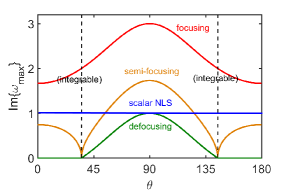
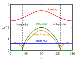
Figure 1: (Color Online) Top: The maximum growth rate vs. the ellipticity angle $\theta$. Bottom: The critical wave number, $k_{c},$ vs. the ellipticity angle $\theta$. The dashed vertical lines identify the integrable $(g=1)$ case.

Interestingly, both values are maximized for circular birefringence, i.e. for $\theta=90^{\circ}$ and take their minimum values for linear birefringence $\theta=0^{\circ}$. This means that for $\theta=90^{\circ}$ the instability will occur sooner and there also more wavenumbers for which the system is unstable. Furthermore, as seen from these figures, the coupled system differs significantly from its scalar counterpart. Indeed, in the focusing case the MI growth rate is larger than the corresponding scalar NLS equation, while in the defocusing case the system can be modulationally unstable (for some angles) with growth rates comparable to its scalar focusing analogue. What is also important for our study, is that, in general, the coupled semi-focusing system exhibits higher growth rates and the range of unstable wavenumbers is also significantly wider than the scalar focusing system. That, typically, would suggest that the coupled system should exhibit more rogue events as it is more unstable.

To test this, we integrate numerically (1) using a pseudospectral method in space and exponential Runge-Kutta for the evolution kassam in a computational domain $t\in[-100,100]$, $z\in[0,20]$. An appropriate initial condition would be a wide gaussian of the form

$$u(t,0)=v(t,0)=e^{-t^{2}/2\sigma^{2}},\;\sigma=30$$

perturbed with 10% random noise; random noise ensures that initially the two conditions will always be different so that the system would not degenerate to the case $u\equiv v$. A wide gaussian with randomness added is a prototype of a set of broad/randomly generated states which can potentially excite more that one wave numbers as it can be regarded as a Fourier series of different cw waves of different $k$’s. For each polarization angle $\theta$ we perform $10^{5}$ trials. In each trial we measure the highest wave amplitude and introduce the quantity

$$\eta(t,z)=\sqrt{\frac{{|u(t,z){|^{2}}+|v(t,z){|^{2}}}}{\max\{|u(t,0){|^{2}}+|v(t,0){|^{2}}\}}}$$

which is the ratio of the highest combined wave amplitude (complex electromagnetic field) to the maximum of the initial condition. This measures the relative growth in amplitude from an initial state. Here we consider a rogue event as one in which $\eta(t,z)$ at some value of $z$ is at least three times its maximum initial value.

We show in Fig. 2, for $\theta=90^{\circ}$ where all critical values are maximized, the probability density functions (PDFs) for all three cases and the results for the scalar NLS equation.

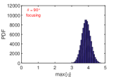
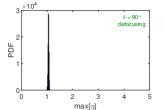
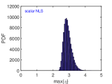
Figure 2: (Color Online) The PDFs for the highest growth rate angle, $\theta=90^{\circ}$, and the corresponding scalar system.

These PDFs indicate that for the focusing system at $\theta=90^{\circ}$ the mean value of the distribution has a significant shift towards larger values, as compared to the scalar NLS equation. On the other hand the results from the semi-focusing and defocusing cases do not show a similar shift under the same comparison. Indeed, in the semi-focusing case the maximum growth rate is higher than the scalar system while in the defocusing case they are equal. However, in the semi-focusing case the mean is shifted towards smaller values as compared to the scalar case, and in the defocusing case there are no rogue events.

To further investigate the above observation, we perform the same analysis for different values of $\theta$. In Fig. 3 we depict the change of the mean value of rogue events with $\theta$ as well as the change of the top $10$% of the highest valued events. As clearly seen, rogue events do not follow the common belief that they are intimately related to the MI growth rates.

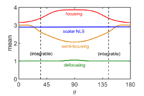
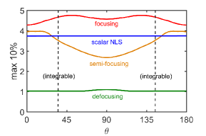
Figure 3: (Color Online) The mean value of the PDFs (top) and the mean value of the max 10% events (bottom) with the the ellipticity angle $\theta$. The dashed lines correspond to the integrable $(g=1)$ case.

There are essentially three distinct cases here, which are not distinguished by the relative MI analysis. The three cases refer to the three different systems: focusing, semi-focusing and defocusing. In the first case, there is a significant increase in the number and severity of rogue events; this is consistent with the increase in the growth rates and size of the instability region. However, in the approximate region $60^{\circ}<\theta<90^{\circ}$, the mean remains essentially stable. The picture is different with regard to the maximum events where there is a slight decrease. Overall, however, in the pure focusing case there is a significant increase in both the number and severity of events. On the other hand, in the defocusing case, the number of rogue events is essentially negligible.

This contradicts the observation that for $35^{\circ}<\theta<90^{\circ}$ the system is unstable with nontrivial growth rates and in turn the belief that this should result into more rogue events. In the semi-focusing case, while the growth rates are increasing for these values of $\theta$ both the mean and max values are decreasing. In fact, the system exhibits a minimum mean and max values for $\theta=90^{\circ}$ while both $\mathrm{Im}\{\omega_{\mathrm{max}}\}$ and $k_{c}$ are maximized. Furthermore, the scalar NLS equation exhibits larger mean values and maxima for a wide range of angles. These observations clearly contradict the belief that higher MI growth rates should lead to more numerous rogue waves; these results are in agreement with the observations of Ref. horikis in deep water waves.

Lastly, we exploit the nature of these rogue events. This also helps provide additional context to the above observations. We focus only on the two focusing and semi-focusing cases where rogue waves are found. We fix the ellipticity angle to $\theta=90^{\circ}$ and zoom in around a typical maximum event in both components of the field $u$ and $v$. We begin with the focusing case, in Fig. 4.

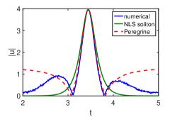
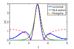
Figure 4: (Color Online) The maximum wave amplitude for the focusing case ($\theta=90^{\circ}$). The numerical observation is fitted against the Peregrine and single soliton solutions of (3).

In this case, we observe that a very good fit to a typical rogue event is described by the scalar NLS equation

$$i\frac{{\partial u}}{{\partial z}}+\frac{{{d}}}{2}\frac{{{\partial^{2}}u}}{{\partial{t^{2}}}}+(g+1)|u|^{2}u=0$$ (3)

where $d_{1}=d_{2}=d$ and $u\equiv v$. This equation admits the so-called Peregrine soliton peregrine

$$u(t,z)={u_{0}}\left[{1-\frac{{2d[1+2i(g+1)u_{0}^{2}z]}}{{d/2+2d{{(g+1)}^{2}}u_{0}^{2}{z^{2}}+2(g+1)u_{0}^{2}{t^{2}}}}}\right]{e^{i(gu_{0}^{2})z}}$$ (4)

while the corresponding single soliton solution reads

$$u(t,z)={u_{0}}{\rm sech}\left(\sqrt{(g+1)/d}{u_{0}}t\right){e^{i[(g+1)u_{0}^{2}/2]z}}.$$ (5)

The free parameter $u_{0}$ represents the amplitude of the wave in both cases.

This situation can occur because the reduction $u=v$ is possible in this case as (1) are symmetric. On the other hand when the system is not symmetric, $d_{1}=-d_{2}$, the computations indicate that the first component ($u$) does not contribute significantly to the rogue wave formation and the rogue event is well approximated by the solitonic solution (5). We see this exemplified in Fig. 5.

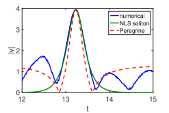
Figure 5: (Color Online) The maximum wave amplitude for the semi-focusing case ($\theta=90^{\circ}$). The numerical observation is fitted against the Peregrine and single soliton solutions of (3).

Furthermore the largest rogue events seem to occur when both equations are unstable, i.e. when both contribute to the formation of extreme events. In this case, the rogue wave is well approximated (for the symmetric system) by the rational solution, (4). On the other hand, when symmetry is lost and only one equation dominates the rogue wave formation, the resulting wave is a soliton of the respective unstable scalar equation, (5). This is also consistent with the findings of Ref. horikis , where in the unstable case the rogue waves were well approximated by hyperbolic secants; they did not exhibit algebraic decay.

To conclude, we have studied the occurrence of rogue waves in birefringent optical fibers. For certain parameter regimes, in the focusing case, e.g. in the circularly birefringent case ($\theta=90^{\circ}$), a major increase in the number of rogue events results from the CNLS system as compared to the scalar NLS equation; this correlates with an increase in the growth rate and size of the MI region. But larger MI growth rates do not always lead to more rogue events: i.e. in the defocusing and semi-focusing cases. Furthermore, we find that the Peregrine soliton is only a good approximation of the focusing CNLS system when the rogue event in both components are nearly equal and, in turn, the system is approximated by the reduced scalar NLS equation. In the semi-focusing case rogue events are such that the defocusing component is negligible and the semi-focusing CNLS system reduces to the scalar focusing NLS equation; here the event is well approximated by the one soliton solution of the relative NLS equation.

MJA is partially supported by NSF under Grant DMS-1310200.

References

- (1) A. Slunyaev, C. Kharif, and E. Pelinovsky, Rogue Waves in the Ocean (Spinger, 2009).
- (2) D. R. Solli, C. Ropers, P. Koonath, and B. Jalali, Nature Lett. 450, 1054 (2007).
- (3) M. J. Ablowitz, Nonlinear Dispersive Waves (Cambridge University Press, 2011).
- (4) M. Erkintalo, K. Hammani, B. Kibler, C. Finot, N. Akhmediev, J. M. Dudley, and G. Genty, Phys. Rev. Lett. 107, 253901 (2011).
- (5) J. M. Dudley, F. Dias, M. Erkintalo, and G. Genty, Nature Photonics 8, 755 (2014).
- (6) J. M. Dudley, M. Erkintalo, and G. Genty, Opt. Photon. News 26, 34 (2015).
- (7) S. Trillo, S. Wabnitz, R. H. Stolen, G. Assanto, C. T. Seaton, and G. I. Stegeman, Appl. Phys. Lett. 49, 1224 (1986).
- (8) S. Trillo and S. Wabnitz, Opt. Lett. 16, 986 (1991).
- (9) V. E. Zakharov and L. A. Ostrovsky, Physica D 238, 540 (2009).
- (10) G. P. Agrawal, Nonlinear Fiber Optics (Academic Press, 2013).
- (11) Y. S. Kivshar and G. P. Agrawal, Optical Solitons: From Fibers to Photonic Crystals (Academic Press, 2003).
- (12) S. Trillo, S. Wabnitz, E. M. Wright, and G. I. Stegeman, Opt. Lett. 13, 871 (1988).
- (13) V. E. Zakharov, A. I. Dyachenko, and A. O. Prokofiev, Eur. J. Mech. B Fluids 25, 677 (2006).
- (14) V. E. Zakharov and A. A. Gelash, Phys. Rev. Lett. 111, 054101 (2013).
- (15) N. Akhmediev, J. M. Soto-Crespo, and A. Ankiewicz, Phys. Rev. A 80, 043818 (2009).
- (16) M. Onorato, S. Residoric, U. Bortolozzoc, A. Montinad, and F. T. Arecchie, Phys. Reports 528, 47 (2013).
- (17) F. Baronio, S. Chen, P. Grelu, S. Wabnitz, and M. Conforti, Phys. Rev. A 91, 033804 (2015).
- (18) M. Onorato, D. Proment, and A. Toffoli, Phys. Rev. Lett. 107, 184502 (2011).
- (19) M. Onorato, A. R. Osborne, and M. Serio, Phys. Rev. Lett. 96, 014503 (2006).
- (20) M. J. Ablowitz and T. P. Horikis, Phys. Fluids 27, 012107 (2015).
- (21) F. Baronio, M. Conforti, A. Degasperis, and S. Lombardo, Phys. Rev. Lett. 111, 114101 (2013).
- (22) F. Baronio, A. Degasperis, M. Conforti, and S. Wabnitz, Phys. Rev. Lett. 109, 044102 (2012).
- (23) F. Baronio, M. Conforti, A. Degasperis, S. Lombardo, M. Onorato, and S. Wabnitz, Phys. Rev. Lett. 113, 034101 (2014).
- (24) D. H. Peregrine, J. Austral. Math. Soc. Ser. B 25, 16 (1983).
- (25) N. N. Akhmediev, V. M. Eleonskii, and N. E. Kulagin, Theoret. and Math. Phys. 72, 809 (1987).
- (26) N. Akhmediev, J. M. Soto Crespo, and A. Ankiewicz, Phys. Lett. A 373, 2137 (2009).
- (27) A. Kassam and L. N. Trefethen, SIAM J. Sci. Comput. 26, 1214 (2005).