NLO electroweak corrections to off-shell top–antitop production with leptonic decays at the LHC

Abstract

For the first time the next-to-leading-order electroweak corrections to the full off-shell production of two top quarks that decay leptonically are presented. This calculation includes all off-shell, non-resonant, and interference effects for the 6-particle phase space. While the electroweak corrections are below one percent for the integrated cross section, they reach up to $15\%$ in the high-transverse-momentum region of distributions. To support the results of the complete one-loop calculation, we have in addition evaluated the electroweak corrections in two different pole approximations, one requiring two on-shell top quarks and one featuring two on-shell W bosons. While the former deviates by up to $10\%$ from the full calculation for certain distributions, the latter provides a very good description for most observables. The increased centre-of-mass energy of the LHC makes the inclusion of electroweak corrections extremely relevant as they are particularly large in the Sudakov regime where new physics is expected to be probed.

1 Introduction

The top quark is the heaviest elementary particle known so far and decays before it hadronises. Its examination is of prime importance at the Large Hadron Collider (LHC) Chatrchyan:2012bra ; Chatrchyan:2013faa ; Aad:2014kva ; Khachatryan:2015uqb ; delDuca:2015gca ; Aaboud:2016pbd . Therefore its production and decay rate should be computed and measured with the highest possible precision. In that respect, not only next-to-leading-order (NLO) QCD corrections Nason:1989zy ; Beenakker:1990maa ; Mangano:1991jk ; Frixione:1995fj ; Bernreuther:2004jv ; Melnikov:2009dn ; Bernreuther:2010ny ; Campbell:2012uf ; Denner:2010jp ; Bevilacqua:2010qb ; Denner:2012yc ; Frederix:2013gra including parton-shower matching Frixione:2003ei ; Frixione:2007nw ; Hoeche:2014qda ; Garzelli:2014dka ; Campbell:2014kua ; Jezo:2016ujg but also next-to-next-to-leading-order (NNLO) QCD Czakon:2013goa ; Czakon:2016ckf ; Czakon:2016dgf , resummation Beneke:2009rj ; Czakon:2009zw ; Ahrens:2010zv ; Kidonakis:2009ev ; Kidonakis:2010dk , and NLO electroweak (EW) corrections Beenakker:1993yr ; Bernreuther:2005is ; Kuhn:2005it ; Moretti:2006nf ; Kuhn:2006vh ; Bernreuther:2006vg ; Hollik:2007sw ; Bernreuther:2008aw ; Bernreuther:2008md ; Beneke:2015lwa ; Pagani:2016caq must be considered. The latter have so far exclusively been computed for on-shell top quarks. We fill this gap by computing for the first time the EW corrections to the full off-shell production of two top quarks that decay leptonically. Because typical EW corrections are of the order of the NNLO QCD ones, they must be included in any precise analysis. Moreover, they can grow large in particular regions of the phase space such as for large transverse momenta. This is particularly relevant, as for run II the LHC is performing at a never accessed centre-of-mass energy. The EW corrections are specifically relevant in the tails of distributions where new-physics contributions are expected to appear. Thus, EW corrections constitute a non-negligible Standard Model background in the phase-space regions relevant for new-physics searches Frederix:2007gi ; Bernreuther:2015fts ; Greiner:2014qna ; Backovic:2015soa ; Arina:2016cqj ; Hespel:2016qaf . Improving the Standard Model predictions allows to further constrain new-physics models or could reveal discrepancies with experimental measurements.

In this article, the first calculation of the full NLO EW corrections to the hadronic production of a positron, a muon, missing energy, and two bottom-quark jets, i.e. $\text{p}\text{p}\to\text{e}^{+}\nu_{\text{e}}\mu^{-}\bar{\nu}_{\mu}\text{b}\bar{\text{b}}$, at the LHC is reported. This final state is dominated by the production of a pair of top quarks that then subsequently decay leptonically. In particular, all off-shell, non-resonant, and interference effects are taken into account. Moreover, the dominant photon-initiated process is included for reference.

In order to support our findings we have compared the full computation to two approximate ones. Namely, we have also computed the EW corrections in a double-pole approximation (DPA) with two resonant W bosons and one with two resonant top quarks following the methods of Refs. Denner:2000bj ; Accomando:2004de . This technique has been shown to be useful in the past when computing EW corrections to Drell–Yan processes Wackeroth:1996hz ; Baur:1998kt ; Dittmaier:2001ay as well as di-boson production Jadach:1996hi ; Denner:1997ia ; Jadach:1998tz ; Beenakker:1998gr ; Chapovsky:1999kv ; Denner:2000bj ; Bredenstein:2005zk ; Billoni:2013aba . It has the advantage that it does not require the knowledge of the full virtual corrections which usually constitutes the bottleneck of this type of computations. Nonetheless one can approximate the full virtual corrections with an accuracy of few per cent with respect to the leading-order (LO) contribution for many observables. This accuracy is often below the experimental resolution, and thus the pole approximation is sufficient. Recently, the EW non-factorisable corrections needed for pole approximations have been derived in a general form in Ref. Dittmaier:2015bfe , and these results have been used extensively in the present work. We thus assess the quality of two DPAs for the production of off-shell top quarks, which is so far the most complicated process where it has been applied.

From a technical points of view, this computation has been made possible thanks to two ingredients. First the implementation of powerful in-house multi-channel Monte Carlo program MoCaNLO . The second aspect is the use of the fast and reliable matrix-element generator Recola Actis:2012qn ; Actis:2016mpe at the Born and one-loop level. This set-up allows us to compute processes with a complexity equal to or higher than the state-of-the-art NLO calculations Denner:2015yca ; Bevilacqua:2015qha ; Kallweit:2015dum ; Cordero:2015hem ; Biedermann:2016yvs ; Biedermann:2016guo .

This article is organised as follows: in Section 2 the set-up of the calculation is specified. In particular, details about the real (Section 2.1) and virtual (Section 2.2) corrections are provided. The two DPAs considered are introduced in Section 2.3, and the checks we have performed are exposed in Section 2.4. Finally, in Section 3 numerical results are presented for a centre-of-mass energy of $\sqrt{s}=13\,\text{TeV}$ at the LHC. More specifically, in Section 3.1 the input parameters and selection cuts are specified. The results for integrated cross sections and distributions appear in Section 3.2 and Section 3.3, respectively. In Section 3.4 the full calculation and the DPAs are compared both at the level of the total cross section and of distributions. Our concluding remarks appear in Section 4.

2 Details of the calculation

In this article, the EW corrections to the full hadronic process

$$\text{p}\text{p}\to\text{e}^{+}\nu_{\text{e}}\mu^{-}\bar{\nu}_{\mu}\text{b}\bar{\text{b}}$$ (1)

are considered. The tree-level matrix element squared contributes at the order $\mathcal{O}{\left(\alpha_{\text{s}}^{2}\alpha^{4}\right)}$. The EW corrections to this process comprise all possible corrections of the order $\mathcal{O}{\left(\alpha_{\text{s}}^{2}\alpha^{5}\right)}$. Moreover, the tree-level $\gamma{\rm g}$ contributions which are of the order $\mathcal{O}{\left(\alpha_{\text{s}}\alpha^{5}\right)}$ have been included for reference. In principle one should also take into account the QCD corrections to these contributions which are of the order $\mathcal{O}{\left(\alpha_{\text{s}}^{2}\alpha^{5}\right)}$. Since the $\gamma{\rm g}$ channel contributes only at the level of a per cent, the corresponding QCD corrections, which form a gauge-independent subset, are expected to be at the per-mille level with respect to the LO of the process (1) and have therefore been neglected. In the present calculation all interferences, resonant, non-resonant, and off-shell effects of the top quarks as well as the gauge bosons are taken into account. In Figure 1 some diagrams for two, one, and no resonant top quark(s) are displayed. Note that the quark-mixing matrix has been assumed to be diagonal. Moreover, the contributions originating from the bottom-quark parton distribution function (PDF) have been neglected.

Figure 1: Representative tree-level Feynman diagrams with two (left), one (middle) and no (right) top-quark resonances.

The calculation is performed with the in-house multi-channel Monte Carlo program MoCaNLO MoCaNLO which has proven to be particularly suited for complicated processes with high multiplicity Denner:2015yca . It uses phase-space mappings similar to those of Refs. Berends:1994pv ; Denner:1999gp ; Dittmaier:2002ap . Infrared (IR) singularities in the real contributions are handled by the dipole subtraction method Catani:1996vz ; Dittmaier:1999mb ; Catani:2002hc ; Phaf:2001gc implemented in a general manner for both QCD and QED. The matrix-element generator Recola-1.0 Actis:2012qn ; Actis:2016mpe and the loop-integral library Collier-1.0 Denner:2014gla ; Denner:2016kdg have been linked to the Monte Carlo code. They are used for the computation of all tree and one-loop amplitudes and all ingredients needed for the subtraction terms such as colour- and spin-correlated squared amplitudes. The calculation presented here is similar to those for $\text{p}\text{p}\to\text{e}^{+}\nu_{\text{e}}\mu^{-}\bar{\nu}_{\mu}\text{b}\bar{\text{b}}\text{H}$ in Ref. Denner:2015yca and $\text{p}\text{p}\to\text{e}^{+}\nu_{\text{e}}\mu^{-}\bar{\nu}_{\mu}\text{b}\bar{\text{b}}$ in Ref. Denner:2012yc in many respects. In particular, the selection cuts considered are almost identical, and the same computer programs have been used as in Ref. Denner:2015yca .

2.1 Real corrections

The real corrections comprise all the real-radiation contributions of order $\mathcal{O}{\left(\alpha_{\text{s}}^{2}\alpha^{5}\right)}$ to the process (1). The first type of real corrections is due to photons radiated from any of the charged particles involved in the tree-level process $\text{p}\text{p}\to\text{e}^{+}\nu_{\text{e}}\mu^{-}\bar{\nu}_{\mu}\text{b}\bar{\text{b}}$. As we are aiming at the complete $\mathcal{O}{\left(\alpha_{\text{s}}^{2}\alpha^{5}\right)}$ corrections, interferences of a QCD production of the pair of top quarks and a gluon with its EW counterpart in the ${q\bar{q}}$ channel must be taken into account. Note that because of the colour structure, the only non-zero contributions are the interferences between initial- and final-state radiation diagrams. This is exemplified on the left-hand side of Figure 2. The squared Feynman diagrams are represented in the figure with on-shell top quarks in order to simplify the representation, but the final state considered in the calculation does not involve two on-shell top quarks but rather four leptons and two bottom-quark jets. In the same manner, another type of interference appears, namely the interference in the ${qg}$ or ${\bar{q}g}$ channel as shown on the right-hand side of Figure 2.

Figure 2: Representative real Feynman diagrams squared which feature interference between QCD and EW tree-level diagrams. Only the top quarks are represented as the inclusion of their decay products does not alter the discussion.

For the treatment of the IR singularities, the Catani–Seymour subtraction formalism Catani:1996vz ; Catani:2002hc has been used for QCD and its extension to QED Dittmaier:1999mb . The QCD singularities from collinear initial-state splittings have been absorbed in the PDFs using the $\overline{\text{MS}}$ factorisation scheme. The NNPDF collaboration Ball:2013hta states that the $\mathrm{NNPDF23}\_\mathrm{nlo}\_\mathrm{as}\_0119\_\mathrm{qed}$ PDF sets can be used in any reasonable factorisation scheme for QED, as the QED evolution is taken into account at leading-logarithmic level. Nonetheless the use of different factorisation schemes differs by next-to-leading logarithms, and the perturbative expansion can show better convergence in certain schemes Diener:2005me ; Dittmaier:2009cr . For this reason, the EW collinear initial-state splittings have been handled using the DIS factorisation scheme. The difference between the two schemes turned out to be below the integration error at the total cross-section level. Even if noticeable (around $1\%$) for the quark-induced channels, the difference is negligible for the total cross section as the gg channel (which does not feature initial-state photon radiation) is dominant. Note finally that all the squared amplitudes for the real-correction sub-processes as well as the colour- and spin-correlated squared amplitudes have been obtained from the computer code Recola Actis:2012qn ; Actis:2016mpe .

2.2 Virtual corrections

As for the real corrections, there are two types of virtual corrections. The first type results from the insertion of an EW particle anywhere in the tree-level amplitude. In the $\bar{q}q$ channel, a second type originates from the insertion of a gluon in the QCD-mediated tree-level amplitude which is then interfered with the EW tree-level amplitude. These two types of corrections are depicted in Figure 3. Again only the two top quarks and not their decay products are represented to simplify the discussion. Some exemplary diagrams of the most complicated loop amplitudes (7- and 8-point functions) are depicted in Figure 4. The virtual corrections have been computed in the ’t Hooft–Feynman gauge in dimensional regularisation using the matrix-element generator Recola Actis:2012qn ; Actis:2016mpe as well as the library Collier Denner:2014gla ; Denner:2016kdg , which is used to calculate the one-loop scalar 'tHooft:1978xw ; Beenakker:1988jr ; Dittmaier:2003bc ; Denner:2010tr and tensor integrals Passarino:1978jh ; Denner:2002ii ; Denner:2005nn numerically.

Figure 3: Representative one-loop Feynman diagrams squared. The diagram on the left-hand side represents an EW correction to the QCD process. It can also be interpreted as a QCD correction to the EW amplitude interfered with the QCD amplitude. The right-hand side shows a QCD correction to the QCD amplitude interfered with the EW amplitude. Only the top quarks are represented as the inclusion of their decay products does not alter the discussion.

Figure 4: Representative octagon and heptagon one-loop Feynman diagrams.

All resonant massive particles, i.e. top quarks, Z bosons and W bosons, are treated in the complex-mass scheme Denner:1999gp ; Denner:2005fg ; Denner:2006ic . Accordingly, the masses of the unstable particles as well as the weak mixing angle are consistently treated as complex quantities,

$$\overline{M}^{2}_{\text{W}}=M_{\text{W}}^{2}-\mathrm{i}M_{\text{W}}\Gamma_{\text{W}},\qquad\overline{M}^{2}_{\text{Z}}=M_{\text{Z}}^{2}-\mathrm{i}M_{\text{Z}}\Gamma_{\text{Z}},\qquad\text{and}\qquad\cos\theta_{\mathrm{w}}=\frac{\overline{M}_{\text{W}}}{\overline{M}_{\text{Z}}}.$$ (2)

2.3 Double-pole approximation

Generalities

The dominant contributions to the process $\text{p}\text{p}\to\text{e}^{+}\nu_{\text{e}}\mu^{-}\bar{\nu}_{\mu}\text{b}\bar{\text{b}}$ result from the production of two top quarks that subsequently decay into bottom quarks and W bosons, which in turn decay into lepton–neutrino pairs. The simplest approximation is thus to require two on-shell top quarks and two on-shell W bosons. However, demanding just two on-shell top quarks is not much more complicated, since each decaying top quark gives rise to a W boson anyhow. Requiring in turn only two on-shell W bosons, will thus include also all contributions with resonant top quarks, but in addition also all contributions with one resonant top quark.

Calculating the NLO corrections to a process with intermediate on-shell particles implies to include the corrections to their production and decay. The on-shell approximation does not include off-shell effects as well as virtual corrections that link the production part and the decay parts or different decay parts. Such corrections should be of the order $\mathcal{O}{\left(\Gamma_{i}/M_{i}\right)}$ Fadin:1993kt ; Fadin:1993dz ; Melnikov:1993np if the decay products are treated inclusively and the resonant contributions dominate. Here $\Gamma_{i}$ and $M_{i}$ are the width and the mass of the resonant particles, respectively. Off-shell effects of the resonant particles can be taken into account by using the pole approximation. In this case, the resonant propagators are fully included, while the rest of the matrix element is expanded about the resonance poles. Moreover, spin correlations between production and decay can be included easily.

We have studied two different DPAs for the process (1) graphically represented in Figure 5: In one case, we require two resonant W bosons and in the second case two resonant top quarks. In order to ensure gauge invariance, the momenta of the resonant particles entering the matrix elements have to be projected on shell. On the other hand, in the phase space and in the propagators of the resonant particles off-shell momenta are used. In the DPA, as in any pole approximation, two different kinds of corrections appear, factorisable and non-factorisable corrections.

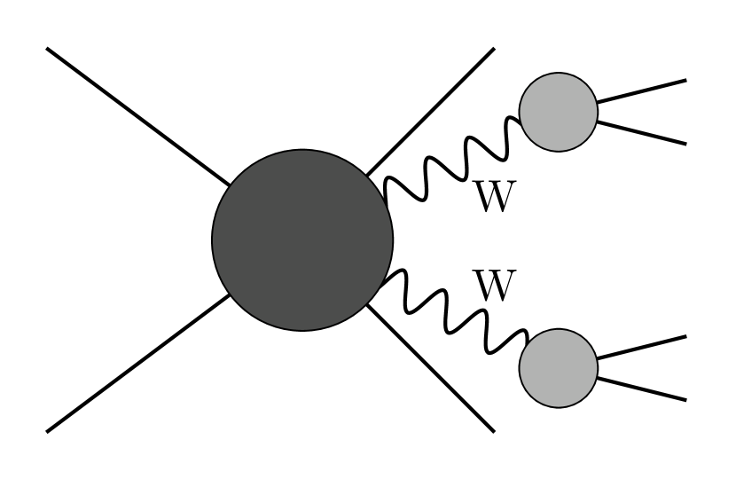
Figure 5: Schematic representation of the two DPAs. On the left-hand side the two W bosons are projected on shell, while on the right-hand side the two top quarks are projected on shell.

The factorisable virtual corrections can be uniquely attributed either to the production of the resonant particles or to their decays. Thus, the diagrams displayed in Figure 4 are, for example, not included in the set of factorisable virtual corrections. Using the notation of Ref. Dittmaier:2015bfe for a pole approximation of $r$ resonances ($r=2$ for a DPA), the latter can be written as

$$\mathcal{M}_{\mathrm{virt,fact,PA}} =\begin{aligned} &\sum_{\lambda_{1},\ldots,\lambda_{r}}\left(\prod^{r}_{i=1}\frac{1}{K_{i}}\right)\Bigg{[}\mathcal{M}^{I\to N,\overline{R}}_{\mathrm{virt}}\prod^{r}_{j=1}\mathcal{M}^{j\to R_{j}}_{\mathrm{LO}}\end{aligned}$$

$$\quad{}+\begin{aligned} &\mathcal{M}^{I\to N,\overline{R}}_{\mathrm{LO}}\sum^{r}_{k=1}\mathcal{M}^{k\to R_{k}}_{\mathrm{virt}}\prod^{r}_{j\neq k}\mathcal{M}^{j\to R_{j}}_{\mathrm{LO}}\Bigg{]}_{\left\{\overline{k}^{2}_{l}\to{\widehat{\overline{k}}}^{2}_{l}=M^{2}_{l}\right\}_{l\in\overline{R}}},\\ \end{aligned}$$ (3)

where $K_{i}=\overline{k}^{2}_{i}-\overline{M}^{2}_{i}$ is the propagator of the resonant particle $i$, with complex mass squared $\overline{M}^{2}_{i}=M^{2}_{i}-\text{i}M_{i}\Gamma_{i}$. The on-shell projection denoted by $\left\{\overline{k}^{2}_{l}\to{\widehat{\overline{k}}}^{2}_{l}=M^{2}_{l}\right\}$ is applied everywhere in the matrix element but in the resonant propagators $K_{i}$. The indices $I$, $\overline{R}$, $R_{i}$ and $N$ denote the ensembles of initial particles, resonant particles, decay products of the resonant particle $i$, and the final-state particles not resulting from the decay of a resonant particle. The polarisations of the resonances are represented by $\lambda_{i}$. Alternatively, the factorisable corrections can be obtained by selecting all Feynman diagrams for the complete process that contain the specified $r$ resonances of the set $\overline{R}$. Using this approach, the factorisable corrections can be generated with the computer code Recola, which allows to select contributions featuring resonances at both LO and NLO.

The factorisable corrections constitute a gauge-invariant subset Stuart:1991xk ; Veltman:1992tm ; Aeppli:1993cb . As virtual corrections, they are not IR finite in the presence of external charged particles. Moreover, taking the on-shell limit of the momenta of the resonant particles introduces additional artificial IR singularities from charged resonances. For example, a photon exchange between a W boson and the attached bottom quark leads to such an artificial IR singularity, if the W boson is projected on shell.

The virtual non-factorisable corrections arise only from diagrams where a photon (or a gluon) is exchanged in the loop Beenakker:1997ir ; Denner:1997ia . On the one hand, they result from manifestly non-factorisable diagrams, i.e. diagrams that do not split into production and decay parts by cutting only the resonant lines, as for example those depicted in Figure 4. On the other hand, they also include contributions from factorisable diagrams. The latter are caused by IR singularities of on-shell resonances. They are obtained by taking the factorisable diagrams, where the IR singularities related to the resonant particles are regularised by the finite decay widths and subtracting these contributions for zero decay width, which contains the artificial IR-divergent piece mentioned previously. In general, the non-factorisable corrections factorise from the LO matrix element and can be written in the form

$$2\mathrm{Re}\left\{\mathcal{M}^{*}_{\mathrm{LO,PA}}\mathcal{M}_{\mathrm{virt,nfact,PA}}\right\}=|\mathcal{M}_{\mathrm{LO,PA}}|^{2}\delta_{\mathrm{nfact}}.$$ (4)

In order to cancel the IR singularities in the virtual corrections, one has to apply the on-shell projection to the terms containing the $I$ operator in the integrated dipole contribution in the same way as for the factorisable and non-factorisable contributions. The $P$- and $K$-operator terms, on the other hand, are evaluated with the off-shell kinematics like the real corrections. This introduces a mismatch, which is of the order of the intrinsic error of the DPA. Note that for the LO and all real contributions no pole approximation is applied Denner:2000bj ; Accomando:2004de .

As mentioned above, in the case of top-quark pair production the ${q\bar{q}}$ channel has two kinds of virtual NLO contributions: the EW loop corrections to the QCD-mediated process and the interference of the QCD-mediated one-loop amplitude with the EW tree amplitude. Both contributions are connected by IR divergences and we call the latter interference contributions in the following. Thus, besides applying the DPA to the EW loop corrections of the QCD-mediated process, we must also adopt the DPA for the second type of corrections. Then, also the corresponding $I$ operator has to be evaluated with on-shell-projected kinematics.

Following the notations of Ref. Dittmaier:2015bfe , all invariants used in the equations below are defined as:

$$s = \left(\sum_{i\in I}p_{i}\right)^{2},$$

$$s_{ij} = \left(k_{i}+k_{j}\right)^{2},\qquad i,j\in I\cup F,$$

$$\overline{s}_{ij} = \left(\overline{k}_{i}+k_{j}\right)^{2},\qquad i\in\overline{R},\qquad j\in I\cup F,$$

$$\widetilde{s}_{ij} = \left(\overline{k}_{i}-k_{j}\right)^{2},\qquad i\in\overline{R},\qquad j\in I\cup F,$$

$$\overline{\overline{s}}_{ij} = \left(\overline{k}_{i}-\overline{k}_{j}\right)^{2},\qquad i,j\in\overline{R},$$ (5)

where the momenta $p_{i}$, $k_{i}$ and $\overline{k}_{i}$ are the momenta of the incoming, outgoing and resonant particles, respectively. Here, $F$ constitutes the ensemble of all the final-state particles.

Double-pole approximation for $\text{W}^{+}$ and $\text{W}^{-}$ bosons

We first discuss the DPA for two W bosons. In order not to shift the top resonances, we have chosen an on-shell projection that leaves the momenta and thus the invariants of the top quarks untouched. Since the $\text{W}^{+}$ boson is projected on its mass shell, one necessarily obtains:

$$p_{\rm t}=p_{\rm b}+{\overline{p}}_{{\rm W}^{+}}=p_{\rm b}+p_{{\rm e}^{+}}+p_{\overline{\nu}_{e}}=\widehat{p}_{\rm b}+{\widehat{\overline{p}}}_{{\rm W}^{+}},$$ (6)

where $\overline{p}$ and $\widehat{p}$ denote the four-momenta of the resonant and the projected particles, respectively. This leads to Dittmaier:2015bfe

$$\widehat{p}_{\rm b}=p_{\rm b}\frac{p^{2}_{\rm t}-m^{2}_{\rm W}}{2p_{\rm b}\cdot p_{\rm t}}\qquad\mathrm{and}\qquad{\widehat{\overline{p}}}_{{\rm W}^{+}}=p_{\rm t}-\widehat{p}_{\rm b}.$$ (7)

In the same manner, the decay products of the resonant $\text{W}^{+}$ boson can be written as

$$\widehat{p}_{{\rm e}^{+}}=p_{{\rm e}^{+}}\frac{m^{2}_{\rm W}}{2p_{{\rm e}^{+}}\cdot{\widehat{\overline{p}}}_{{\rm W}^{+}}}\qquad\mathrm{and}\qquad\widehat{p}_{{\nu}_{e}}={\widehat{\overline{p}}}_{{\rm W}^{+}}-\widehat{p}_{{\rm e}^{+}}.$$ (8)

The kinematic projection for the $\text{W}^{-}$ resonance is obtained by renaming the involved particles.

For the process ${\rm u\overline{u}}\to\text{e}^{+}\nu_{\text{e}}\text{b}\mu^{-}\bar{\nu}_{\mu}\bar{\text{b}}$, the decay products of the ${\rm W}^{+}$ and ${\rm W}^{-}$ bosons are $\text{e}^{+}\nu_{\text{e}}$ and $\mu^{-}\bar{\nu}_{\mu}$, respectively. The final-state particles not resulting from a decay are the two bottom quarks. In the compact notation of Ref. Dittmaier:2015bfe this reads:

$$I=\{1,2\},\qquad R_{1}=\{3,4\},\qquad R_{2}=\{6,7\},\qquad\text{and}\qquad N=\{5,8\}.$$ (9)

The conventions for the sign factors and charges are

$$\sigma_{1}=-\sigma_{2}=1,\qquad\sigma_{3}=\sigma_{7}=\sigma_{8}=1,\qquad\sigma_{4}=\sigma_{5}=\sigma_{6}=-1,$$ (10)

and

$$Q_{1}=Q_{2}=\frac{2}{3},\qquad Q_{3}=Q_{6}=-1,\qquad Q_{4}=Q_{7}=0,\qquad Q_{5}=Q_{8}=-\frac{1}{3}.$$ (11)

The results for the gluon–gluon channel are obtained upon setting $Q_{1/2}=0$.

Owing to the fact that the ensemble $N\cup I$ contains only pairs of particles with opposite charges, the expression for $\delta_{\mathrm{nfact}}$ simplifies to:

$$\delta_{\mathrm{nfact}} =\begin{aligned} &-\sum_{a\in R_{1}}\sum_{b\in R_{2}}\sigma_{a}\sigma_{b}Q_{a}Q_{b}\frac{\alpha}{\pi}\mathrm{Re}\left\{\Delta\left(i=1,a;j=2,b\right)\right\}\end{aligned}$$

$$\quad{}-\begin{aligned} &\sum_{i=1}^{2}\sum_{a\in R_{i}}\sum_{b\in N\cup I}\sigma_{a}\sigma_{b}Q_{a}Q_{b}\frac{\alpha}{\pi}\mathrm{Re}\left\{\Delta_{\mathrm{xf}}\left(i,a;b\right)+\Delta_{\mathrm{xm}}\left(i;b\right)\right\}.\\ \end{aligned}$$ (12)

The different contributions read:

$$\Delta\left(i,a;j,b\right)=\Delta_{\mathrm{mm}}\left(i,j\right)+\Delta_{\mathrm{mf}}\left(i,a;j,b\right)+\Delta_{\mathrm{mm^{\prime}}}\left(i,j\right)+\Delta_{\mathrm{mf^{\prime}}}\left(i,a;j,b\right)+\Delta_{\mathrm{ff^{\prime}}}\left(i,a;j,b\right)$$ (13)

and are further decomposed as

$$\Delta_{\mathrm{mm}}\left(i,j\right) = \Delta^{\prime}_{\mathrm{mm}}\left(i\right)+\Delta^{\prime}_{\mathrm{mm}}\left(j\right),$$

$$\Delta_{\mathrm{mf}}\left(i,a;j,b\right) = \Delta^{\prime}_{\mathrm{mf}}\left(i,a\right)+\Delta^{\prime}_{\mathrm{mf}}\left(j,b\right),$$

$$\Delta_{\mathrm{mf^{\prime}}}\left(i,a;j,b\right) = \Delta^{\prime}_{\mathrm{mf^{\prime}}}\left(i;j,b\right)+\Delta^{\prime}_{\mathrm{mf^{\prime}}}\left(j;i,a\right).$$ (14)

The explicit expressions for the various contributions in terms of scalar integrals can be found in Ref. Dittmaier:2015bfe and have been reproduced for completeness in App. A.

As stated above, the pole approximation should also be applied to the interference contributions. Since we only consider leptonic decays of the W bosons, there are no QCD corrections that link production and decay, and thus no non-factorisable interference contributions appear for the DPA applied to the W bosons. Nonetheless factorisable corrections of interference type exist.

Finally, note that as the width of the W boson is assumed to be zero everywhere except in their resonant propagators, we also set the width of the Z boson to zero. This avoids artificially large higher-order terms in the calculation of the complex weak mixing angle.

Double-pole approximation for t and $\overline{\rm t}$ quarks

Next we discuss the DPA for two top quarks. We use the on-shell projection introduced in Ref. Denner:2014wka and reproduce it here for completeness. In general, one can enforce a projection of two momenta $p_{1}$ and $p_{2}$ such that they fulfil $p_{1}+p_{2}=\widehat{p}_{1}+\widehat{p}_{2}$ with $\widehat{p}_{1}^{2}=m_{1}^{2}$ and $\widehat{p}_{2}^{2}=m_{2}^{2}$, where the masses $m_{1}$ and $m_{2}$ are not necessarily the physical masses. The projected momenta read:

$$\widehat{p}_{1}=\xi p_{1}+\eta p_{2},\qquad\widehat{p}_{2}=(1-\xi)p_{1}+(1-\eta)p_{2}.$$ (15)

The constants $\xi$ and $\eta$ are obtained by solving the quadratic equation

$$0 = \eta^{2}\left[p_{1}^{2}p_{2}-p_{2}^{2}p_{1}+\left(p_{1}p_{2}\right)\left(p_{2}-p_{1}\right)\right]^{2}$$ (16)

$${}+\eta\left[\left(p_{1}+p_{2}\right)^{2}+\widehat{p}^{2}_{1}-\widehat{p}^{2}_{2}\right]\left[\left(p_{1}p_{2}\right)^{2}-p_{1}^{2}p^{2}_{2}\right]$$

$$\times\frac{1}{4}\left[\left(p_{1}+p_{2}\right)^{2}+\widehat{p}^{2}_{1}-\widehat{p}^{2}_{2}\right]^{2}p_{1}^{2}-\left(p_{1}^{2}+p_{1}p_{2}\right)^{2}\widehat{p}^{2}_{1}$$

and using

$$\xi=\frac{\left(\left(p_{1}+p_{2}\right)^{2}+\widehat{p}^{2}_{1}-\widehat{p}^{2}_{2}\right)-2\eta\left(p_{2}^{2}+p_{1}p_{2}\right)}{2\left(p_{1}^{2}+p_{1}p_{2}\right)}.$$ (17)

For the projection of the two top quarks, the only replacements needed are $p_{1}\to\overline{p}_{\rm t}$, $p_{2}\to\overline{p}_{\overline{{\rm t}}}$ and $\widehat{p}^{2}_{1}=\widehat{p}^{2}_{2}=m_{\rm t}^{2}$.

Defining

$$p^{\prime}_{\rm b}=\widehat{\overline{p}}_{\rm t}-p_{{\rm W}^{+}},$$ (18)

it is possible to obtain $\widehat{p}_{\rm b}$ and $\widehat{p}_{{\rm W}^{+}}$ using Eqs. (15)–(17) upon performing the replacements $p_{1}\to p^{\prime}_{\rm b}$ and $p_{2}\to p_{{\rm W}^{+}}$. The projected invariants are defined as $\widehat{p}^{2}_{1}=0$ and $\widehat{p}^{2}_{2}=p^{2}_{{\rm W}^{+}}$. The last condition ensures that the off-shell invariant of the ${\rm W}^{+}$ boson is left untouched (as the top-quark invariants in the on-shell projection with two W bosons explained above). The projection of the antibottom quark and ${\text{W}}^{-}$ boson can be constructed in the same way. The decay products of the $\text{W}^{+}$ boson (in a similar way to what has been done for the previous on-shell projection) read:

$$\widehat{p}_{{\rm e}^{+}}=p_{{\rm e}^{+}}\frac{p^{2}_{{\rm W}^{+}}}{2\widehat{p}_{{\rm W}^{+}}p_{{\rm e}^{+}}},\qquad\widehat{p}_{\nu_{e}}=\widehat{p}_{{\rm W}^{+}}-\widehat{p}_{{\rm e}^{+}}.$$ (19)

The decay products of the ${\rm W}^{-}$ boson can be handled in the same way.

Concerning the non-factorisable corrections, the notations differ slightly from the case considered in Eqs. (9)–(12). In particular, the ensembles of initial-state, decay-product, and remaining final-state particles are:

$$I=\{1,2\},\qquad R_{1}=\{3,4,5\},\qquad R_{2}=\{6,7,8\},\qquad\text{and}\qquad N=\text{\O}.$$ (20)

The convention for the sign factors and charges is as in Eqs.  (10) and (11). The expression for $\delta_{\mathrm{nfact}}$ is still the same as in Eq. (12), only the content of the ensembles $R_{i}$ and $N\cup I$ is modified.

Concerning the interference contributions, as for the case of the WW DPA, the factorisable corrections and the $I$-operator terms have to be computed to in the pole approximation. Here, non-factorisable corrections appear as there are QCD corrections linking the production part and decay part of the top quarks. These non-factorisable QCD corrections can be computed in the same manner as the EW ones. To do this, one replaces the charges and matrix elements squared by the colour-correlated matrix elements squared in Eq. (12). The non-factorisable QCD contribution thus reads:

$$2\mathrm{Re}\biggl{\{}\mathcal{M}^{*}_{\mathrm{LO,PA}} \mathcal{M}_{\mathrm{virt,nfact,PA}}^{\mathrm{QCD}}\biggr{\}}=\begin{aligned} &-\sum_{a\in R_{1}}\sum_{b\in R_{2}}\overline{\mathcal{A}^{2}_{\mathrm{c}}}\left(a,b\right)Q^{\mathrm{c}}_{a}Q^{\mathrm{c}}_{b}\frac{\alpha}{\pi}\mathrm{Re}\left\{\Delta\left(i=1,a;j=2,b\right)\right\}\end{aligned}$$

$$\quad{}-\begin{aligned} &\sum_{i=1}^{2}\sum_{a\in R_{i}}\sum_{b\in N\cup I}\overline{\mathcal{A}^{2}_{\mathrm{c}}}\left(a,b\right)Q^{\mathrm{c}}_{a}Q^{\mathrm{c}}_{b}\frac{\alpha}{\pi}\mathrm{Re}\left\{\Delta_{\mathrm{xf}}\left(i,a;b\right)+\Delta_{\mathrm{xm}}\left(i;b\right)\right\},\\ \end{aligned}$$ (21)

where $\overline{\mathcal{A}^{2}_{\mathrm{c}}}\left(a,b\right)$ denotes the colour-correlated squared amplitude between particle $a$ and $b$ as defined in Ref. Actis:2016mpe . The charges $Q^{\mathrm{c}}_{a/b}$ take the value 1 or 0 if the particle carries a colour charge or not, respectively.

2.4 Validation

Several checks have been performed on this computation. All tree-level, i.e. Born and real, matrix elements squared have been compared with the code MadGraph5_aMC@NLO Alwall:2014hca . Out of 4000 phase-space points, more than 99.9 $\%$ agree to 11 and 10 digits for the Born and real matrix elements squared, respectively. All hadronic Born cross sections (gg, $\bar{q}q$ and $\text{g}\gamma$ channels) have been compared with MadGraph5_aMC@NLO, and agreement within the integration error has been found.

IR und ultra-violet (UV) finiteness have been verified by calculating the cross section for different IR and UV regulators, respectively. The implementation of the dipole subtraction method has been checked by varying the $\alpha$ parameter from $10^{-2}$ to 1. The parameter $\alpha$ allows one to improve the numerical stability of the integration by restricting the phase space for the dipole subtraction terms to the vicinity of the singular regions Nagy:1998bb .

The virtual corrections have been scrutinised in several ways. First, the computer code Recola allows for an internal check of a Ward identity. One can substitute the polarisation vector of one of the initial-state gluons by its momentum normalised to its energy, i.e. $\epsilon^{\mu}_{\text{g}}\to p^{\mu}_{\text{g}}/p^{0}_{\text{g}}$, in the one-loop amplitude. The cumulative fraction of events with $\mathop{\mathrm{Re}}\nolimits\mathcal{M}^{*}_{0}(\epsilon_{\text{g}})\mathcal{M}_{1}(\epsilon_{\text{g}}\to p_{\text{g}}/p^{0}_{\text{g}})/\mathop{\mathrm{Re}}\nolimits\mathcal{M}^{*}_{0}(\epsilon_{\text{g}})\mathcal{M}_{1}(\epsilon_{\text{g}})>\Delta$ is plotted in Fig. 6. It gives results comparably good to those of Ref. Denner:2015yca for $\text{p}\text{p}\to\text{e}^{+}\nu_{\text{e}}\mu^{-}\bar{\nu}_{\mu}\text{b}\bar{\text{b}}\text{H}$ where the median is also around $10^{-9}$. Second, thanks to the two libraries implemented in the computer code Collier, we have been able to estimate the potential error induced when evaluating the virtual corrections. This turned out to be below the per-mille level after integration, i.e. below the precision of integration we have required for the numerical results. Finally, the excellent agreement found with one of the two DPAs (see below) for the observables computed confirms that the full one-loop amplitudes used in this computation are reliable. Note that we have checked also our implementation of the (double-)pole approximation for a variety of processes ranging from Drell–Yan (with W and Z boson) to di-boson production (also involving W or Z bosons).

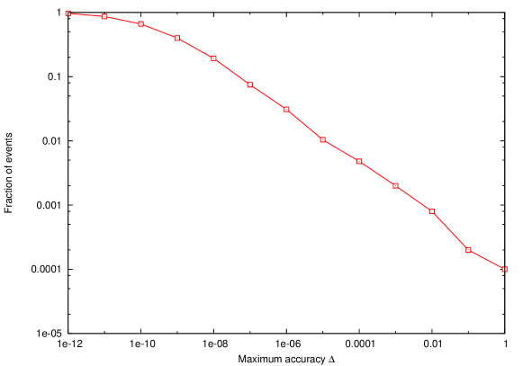
Figure 6: Cumulative fraction of events with a relative accuracy larger than $\Delta$ for $\text{p}\text{p}\to\text{e}^{+}\nu_{\text{e}}\mu^{-}\bar{\nu}_{\mu}\text{b}\bar{\text{b}}$ at NLO EW.

3 Numerical Results

3.1 Input parameters and selection cuts

In this section, integrated cross sections and differential distributions including NLO EW corrections for the LHC at a centre-of-mass energy $\sqrt{s}=13\,\text{TeV}$ are presented. For the parton distribution functions, LHAPDF 6.1.5 Andersen:2014efa ; Buckley:2014ana has been employed. Specifically, the $\mathrm{NNPDF23}\_\mathrm{nlo}\_\mathrm{as}\_0119\_\mathrm{qed}$ set Ball:2013hta ; Carrazza:2013bra ; Carrazza:2013wua at NLO QCD and LO QED has been used for all the LO and NLO contributions. This features the inclusion of a photon PDF needed for the photon-initiated contributions. The strong coupling constant $\alpha_{\text{s}}$ is provided by the PDF set based on a two-loop QCD running with a dynamical flavour scheme with $N_{\text{F}}=6$ active flavours. For the fixed renormalisation and factorisation scale $\mu_{\text{fix}}=m_{\rm t}$, we find

$$\alpha_{\text{s}}(\mu_{\text{fix}})=0.1084656\ldots\;.$$ (22)

Note that contributions for bottom-quark PDFs have been neglected.

Concerning the electromagnetic coupling $\alpha$, the $G_{\mu}$ scheme Denner:2000bj has been used where $\alpha$ is obtained from the Fermi constant,

$$\alpha=\frac{\sqrt{2}}{\pi}G_{\mu}M_{\text{W}}^{2}\left(1-\frac{M_{\text{W}}^{2}}{M_{\text{Z}}^{2}}\right)\qquad\text{with}\qquad G_{\mu}=1.16637\times 10^{-5}\,\text{GeV}.$$ (23)

The input parameters are taken from Ref. Beringer:1900zz , and the numerical values for the masses and widths used in this computation read:

$$m_{\text{t}} =173.34\,\text{GeV}, \quad\quad\quad\Gamma_{\text{t}} =1.36918\ldots\,\text{GeV},$$

$$M_{\text{Z}}^{\text{OS}} =91.1876\,\text{GeV}, \Gamma_{\text{Z}}^{\text{OS}} =2.4952\,\text{GeV},$$

$$M_{\text{W}}^{\text{OS}} =80.385\,\text{GeV}, \Gamma_{\text{W}}^{\text{OS}} =2.085\,\text{GeV},$$

$$M_{\rm H} =125.9\,\text{GeV}.$$ (24)

The masses and widths of all other quarks and leptons have been neglected. We have verified that the effect of a finite bottom-quark mass on the cross section is below the per-cent level in our set-up. The top-quark width has been taken from Ref. Basso:2015gca , where it has been calculated including both EW and QCD NLO corrections for massive bottom quarks. We have found that the effect of the bottom-quark mass on the top-quark width is at the per-mille level by computing the leptonic partial decay width of the top-quark using Ref. Jezabek:1988iv with massive and massless bottom quarks. Such differences are irrelevant with respect to the integration errors for the cross section. We have chosen to use the same top width for our calculation at LO and NLO, since this allows to improve QCD calculations upon multiplying with our results for the relative EW correction factors.

The measured on-shell (OS) values for the masses and widths of the W and Z bosons are converted into pole values for the gauge bosons ($V=\text{W},\text{Z}$) according to Ref. Bardin:1988xt ,

$$M_{V}=M_{V}^{\text{OS}}/\sqrt{1+(\Gamma_{V}^{\text{OS}}/M_{V}^{\text{OS}})^{2}}\,,\qquad\Gamma_{V}=\Gamma_{V}^{\text{OS}}/\sqrt{1+(\Gamma_{V}^{\text{OS}}/M_{V}^{\text{OS}})^{2}}.$$ (25)

The QCD jets are clustered using the anti-$k_{\text{T}}$ algorithm Cacciari:2008gp , which is also used to cluster the photons with light charged particles, with jet-resolution parameter $R=0.4$. The distance between two particles $i$ and $j$ in the rapidity–azimuthal-angle plane is defined as

$$R_{ij}=\sqrt{(\Delta\phi_{ij})^{2}+(y_{i}-y_{j})^{2}},$$ (26)

where $\Delta\phi_{ij}$ is the azimuthal-angle difference. The rapidity of jet $i$ is given by $y_{i}=\frac{1}{2}\ln\frac{E+p_{z}}{E-p_{z}}$ with the energy $E$ of the jet and the component of its momentum along the beam axis $p_{z}$. Only final-state quarks, gluons, and charged fermions with rapidity $|y|<5$ are clustered into IR-safe objects.

After recombination, standard selection cuts on the transverse momenta and rapidities of charged leptons and b jets, missing transverse momentum and rapidity–azimuthal-angle distance between b jets according to Eq. (26) are imposed. In the final state, two b jets and two charged leptons are required, and the following selection cuts are applied:

b jets: $$\qquad p_{\text{T},\text{b}} >25\,\text{GeV}, \qquad|y_{\text{b}}| <2.5,$$

charged lepton: $$p_{\text{T},\ell} >20\,\text{GeV}, |y_{\ell}| <2.5,$$

missing transverse momentum: $$p_{\text{T},\text{miss}} >20\,\text{GeV},$$

b-jet–b-jet distance: $$\Delta R_{\text{b}\text{b}} >0.4.$$ (27)

3.2 Integrated cross section

In this section the results for the integrated cross section are discussed. The different contributions are summarised in Table 1 for the LHC running at a centre-of-mass energy of $\sqrt{s}=13\,\text{TeV}$. It corresponds to the input parameters given in Eqs. (22)–(3.1) , while the selection cuts for this set-up are defined in Eq. (3.1). As stated before, the LO contributions are of the order $\mathcal{O}{\left(\alpha_{\text{s}}^{2}\alpha^{4}\right)}$, while the EW NLO corrections are of the order $\mathcal{O}{\left(\alpha_{\text{s}}^{2}\alpha^{5}\right)}$. Since the ${\rm\gamma g}$ contribution is of the order $\mathcal{O}{\left(\alpha_{\text{s}}\alpha^{5}\right)}$, we have not included them in the definition of the EW NLO corrections. Nonetheless we give it for reference.

Ch.	$\sigma_{\rm LO}$ [fb]	$\sigma_{\rm NLO\;EW}$ [fb]	$\delta$ [$\%$]
gg	$2824.2(2)$	$2834.2(3)$	0.35
${q\bar{q}}$	$375.29(1)$	$377.18(6)$	0.50
${\rm g}q(/\bar{q})$		$0.259(4)$
${\rm\gamma g}$		$27.930(1)$
pp	$3199.5(2)$	$3211.7(3)$	$0.38$

Table 1: Different contributions to the integrated cross section for $\text{p}\text{p}\to\text{e}^{+}\nu_{\text{e}}\mu^{-}\bar{\nu}_{\mu}\text{b}\bar{\text{b}}(\text{j})$ at a centre-of-mass energy of $\sqrt{s}=13\,\text{TeV}$. The quark–antiquark contributions comprise $q=\text{u},\text{d},\text{c},\text{s}$. The channel ${\rm g}q(/\bar{q})$ denotes the real radiation of a quark or an antiquark. In the total cross section (denoted by pp), the photon-induced channel (denoted by ${\rm\gamma g}$) has not been included. The relative correction is defined as $\delta=\sigma_{\rm NLO\;EW}/\sigma_{\rm LO}$. Integration errors of the last digits are given in parentheses.

At the LHC (in contrast to the Tevatron) the gluon–gluon-initiated channel is dominant owing to the enhanced gluon PDF. The ${q\bar{q}}$ channels that comprise ${q}=\text{u},\text{d},\text{c},\text{s}$ are one order of magnitude smaller and represent only $11.7\%$ of the total integrated cross section (both at LO and NLO). The corrections to these two channels are $0.35\%$ and $0.50\%$, respectively. Moreover, the ${\rm g}q/\bar{q}$ channel contributes only at the sub-per-mille level, being of the order of the error on the integrated cross section. The EW corrections to the full partonic process amount to $0.38\%$.

For on-shell top-pair production the EW corrections are usually between $-1\%$ and $-2\%$ (see Ref. Pagani:2016caq for a recent evaluation). This difference to our results can be explained by the EW corrections to the top-quark width that are implicitly contained in our calculation and amount to 1.3% Basso:2015gca . Since we use the same value for the width in the resonant top-quark propagators at LO and NLO, this effect does not cancel. Subtracting twice the relative NLO corrections to the top width from our corrections yields a correction to top-pair production of the usual size.

The ${\rm\gamma g}$ channel gives a contribution of the order of one per cent. Thus, calculating QCD corrections to this partonic channel would lead at most to a per-mille contribution. Nonetheless, the photon-induced channel represents a non-negligible contribution to the cross section.

As stated before we have considered massless bottom quarks and have neglected their PDF contributions. To justify this, we have computed the LO hadronic cross sections including massive bottom quarks and bottom-quark PDFs. The effect of a finite bottom-quark mass is at the level of $0.8\%$. The bottom PDFs contribute at the level of $0.01\%$ to the process $\text{p}\text{p}\to\text{e}^{+}\nu_{\text{e}}\mu^{-}\bar{\nu}_{\mu}\text{b}\bar{\text{b}}$ at LO. This tiny contribution is explained by the dominance of the gluon PDFs.

Thus, the EW corrections are below the per-cent level for the integrated cross section. However, as shown in the next section, this statement does not hold for differential distributions.

3.3 Differential distributions

Turning to differential distributions, we show two plots for each observable. The upper panels display the LO and NLO EW predictions, while the lower panels show the relative correction $\delta=\sigma_{\text{NLO EW}}/\sigma_{\text{LO}}-1$ in per cent. In addition the ${\rm\gamma g}$ contribution is depicted as $\delta_{\rm\gamma g}=\sigma_{\rm\gamma g}/\sigma_{\text{LO}}$ and labelled by photon.

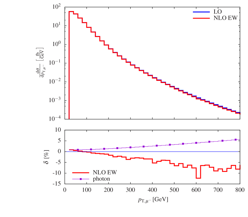
(a)

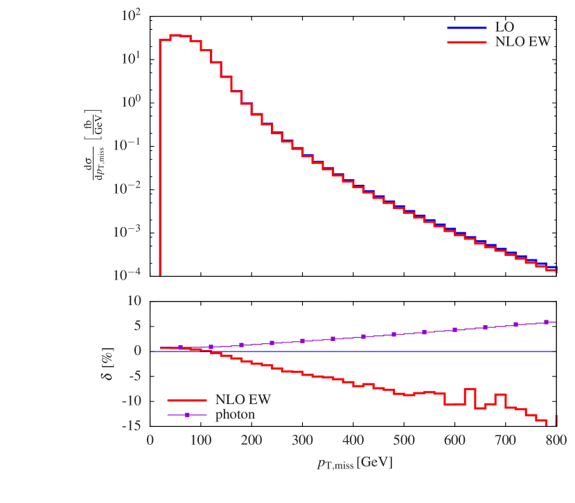
(b)

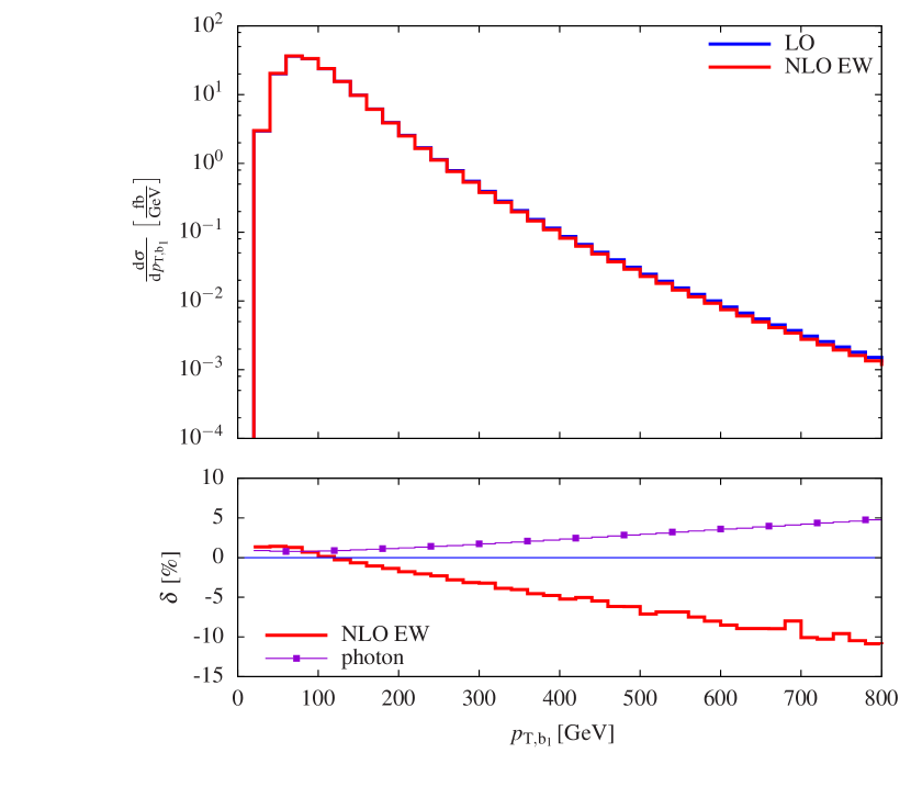
(c)

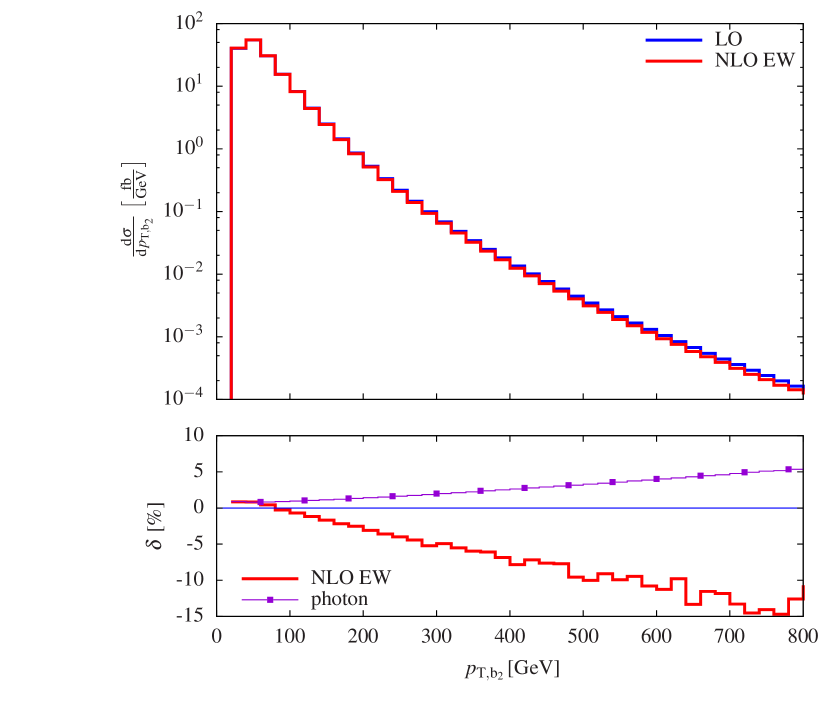
(d)

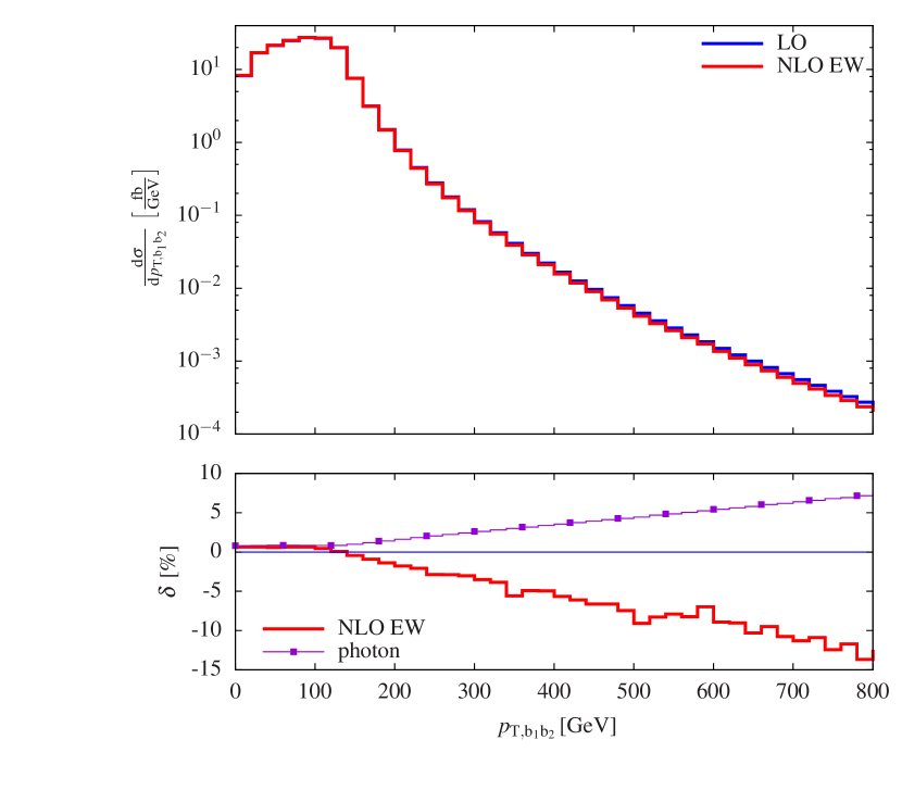
(e)

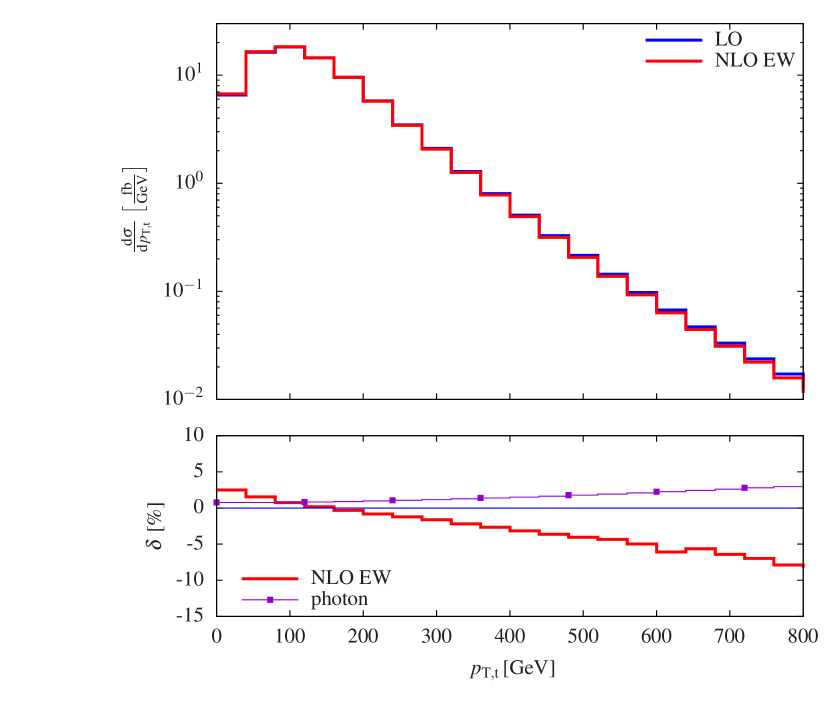
(f)

Figure 7: Transverse-momentum distributions at a centre-of-mass energy $\sqrt{s}=13\,\text{TeV}$ at the LHC: 7(a) for the muon (upper left), 7(b) for missing momentum (upper right), 7(c) for the harder b jet (middle left), 7(d) for the softer b jet (middle right), 7(e) for the b-jet pair (lower left), and 7(f) for the reconstructed top quark (lower right). The lower panel shows the relative NLO EW correction $\delta=\sigma_{\text{NLO EW}}/\sigma_{\text{LO}}-1$ and the relative photon-induced contributions $\delta=\sigma_{\gamma g}/\sigma_{\text{LO}}$ in per cent.

Figure 7(a) displays the distribution of the muon transverse momentum, while Figures 7(c) and 7(d) show the transverse momenta of the harder and softer bottom quark (according to $p_{\text{T}}$ ordering). In Figure 7(b) we present the distribution in the missing transverse momentum, defined as the sum of the transverse momenta of the two neutrinos, i.e. $p_{\text{T},\text{miss}}=\left|\mathbf{p}_{\text{T},\nu_{\text{e}}}+\mathbf{p}_{\text{T},\bar{\nu}_{\mu}}\right|$. The transverse momentum of the bottom-jet pair is displayed in Figure 7(e) and the one of the reconstructed top quark in Figure 7(f). In all distributions in Figure 7 one can clearly see the effects of the Sudakov logarithms at high transverse momenta. In general, the corrections are within $2\%$ for transverse momenta below 50 GeV and grow negative towards high transverse momenta. The EW corrections account for effects of up to $15\%$ over the considered phase-space range up to $800\,\text{GeV}$. In all transverse-momentum distributions, the gluon–photon-induced channel increases towards the high-momentum region. This is due to the fact that the photon PDF grows faster than the quark and gluon PDFs in this region Pagani:2016caq . Indeed, the photon-induced contributions typically reach $5$–$6\%$ at $p_{\text{T}}=800\,\text{GeV}$. But as the photon PDF is still poorly known Carrazza:2013bra ; Ball:2013hta , this statement should be understood with caution. More specifically, in the transverse-momentum distribution of the softer bottom quark, the EW corrections go from $2\%$ at low transverse momentum down to $-15\%$ at 800 GeV. There, the photon-induced channel accounts for $1\%$ at low transverse momentum and up to $5\%$ at 800 GeV.

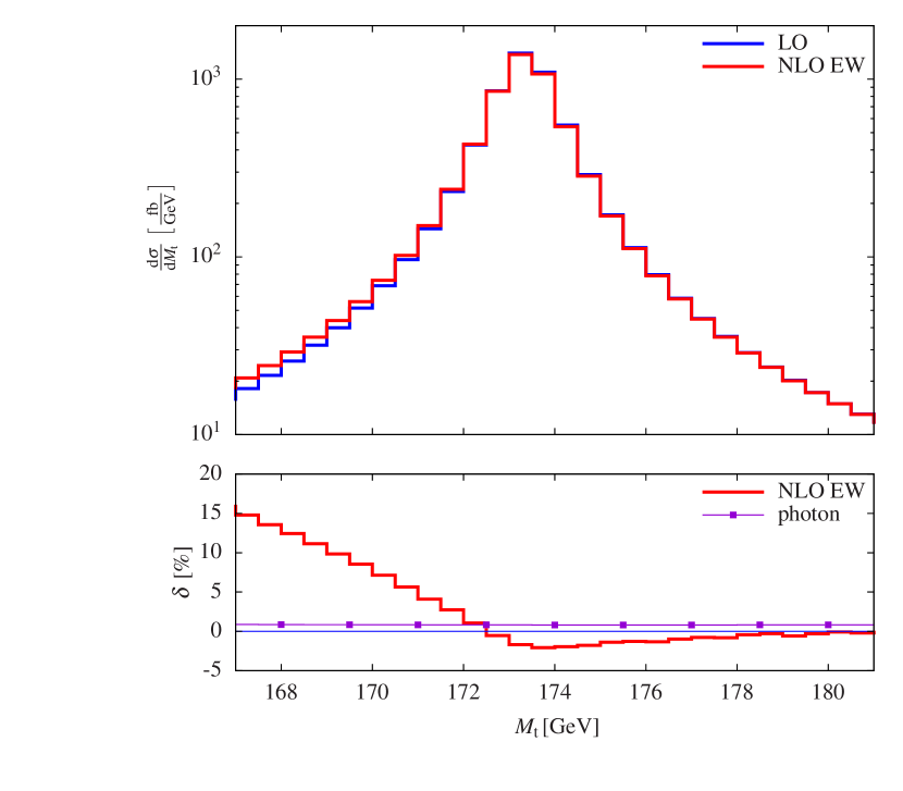
(a)

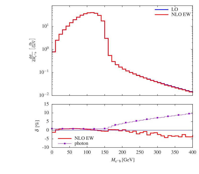
(b)

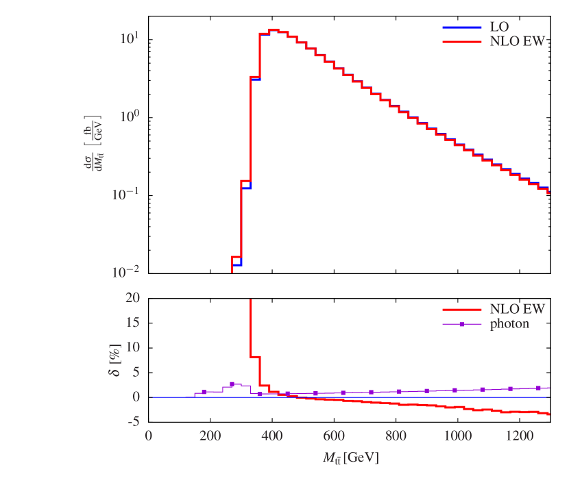
(c)

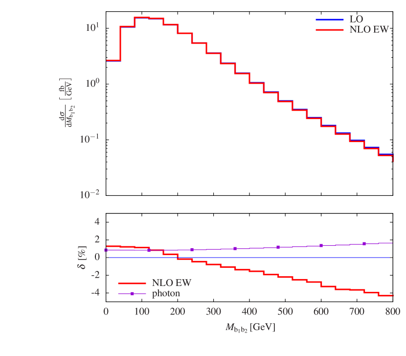
(d)

Figure 8: Differential distributions at a centre-of-mass energy $\sqrt{s}=13\,\text{TeV}$ at the LHC: 8(a) invariant mass of the reconstructed top quark (upper left), 8(b) invariant mass of the $\text{e}^{+}\text{b}$ system (upper right), 8(c) invariant mass of the reconstructed $\text{t}\bar{\text{t}}$ system (lower left), and 8(d) invariant mass of the b-jet pair (lower right). The lower panel shows the relative NLO EW correction $\delta=\sigma_{\text{NLO EW}}/\sigma_{\text{LO}}-1$ and the relative photon-induced contributions $\delta=\sigma_{\gamma g}/\sigma_{\text{LO}}$ in per cent.

In Figure 8, a selection of invariant-mass distributions is shown containing those of the reconstructed top quark (Figure 8(a)), of the $\text{e}^{+}\text{b}$ system (Figure 8(b)), of the reconstructed $\text{t}\bar{\text{t}}$ system (Figure 8(c)), and of the $\text{b}\bar{\text{b}}$ system (Figure 8(d)). Below the top mass, the corrections to the invariant mass of the reconstructed top quark reach up to $15\%$. Such a radiative tail is also observed in similar processes at NLO QCD Denner:2012yc ; Denner:2015yca , and is due to final-state photons (or gluons) that are not reconstructed with the decay products of the top quark. In the distribution in the invariant mass of the positron–bottom-quark system, which is the invariant mass of the visible decay products of the top quark, the LO cross section decreases sharply around $155\,\text{GeV}$. This is due to the existence of an upper bound $M^{2}_{\text{e}^{+}\text{b}}<M^{2}_{\rm t}-M^{2}_{\rm W}\simeq(154\,\text{GeV})^{2}$ for on-shell top quark and W boson. This edge is very sensitive to the top mass and thus allows to determine its experimental value precisely. It marks the transition from on-shell to off-shell top-quark production. In that regard, higher-order corrections to this observable are particularly relevant. At the threshold near $155\,\text{GeV}$, the EW corrections are negative and below one per cent, while the photon-induced contributions reach $1\%$. The corrections below this threshold are of the order of $1\%$. On the other hand, above this bound the EW corrections go down to $-4\%$ for an invariant mass of 400 GeV, while the photon-induced contributions grow to $+10\%$ at $M_{\text{e}^{+}\text{b}}=400\,\text{GeV}$. Thus, the EW corrections and photon-induced contributions should be taken into account. The invariant mass of the $\text{t}\bar{\text{t}}$ system is a very important observable as one could expect new physics in its high-energy tail Frederix:2007gi ; Backovic:2015soa . The corresponding EW corrections are significant and vary from $1\%$ at $400\,\text{GeV}$ to $-4\%$ at $1300\,\text{GeV}$. The invariant mass of the $\text{b}\bar{\text{b}}$ system also displays typical EW corrections, accounting for a $5\%$ variation over the considered range, accompanied by a relatively small photon-induced contribution below $2\%$.

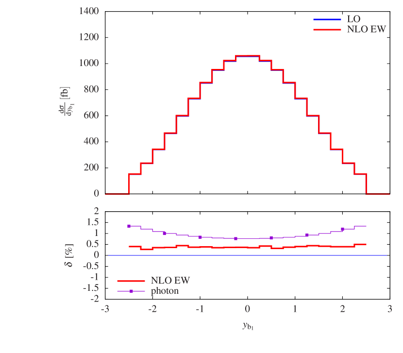
(a)

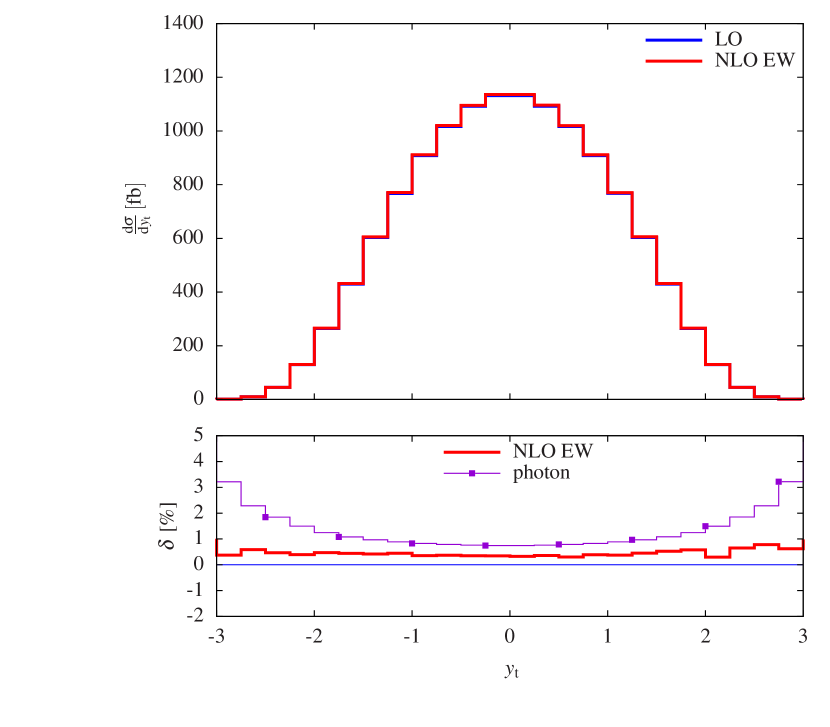
(b)

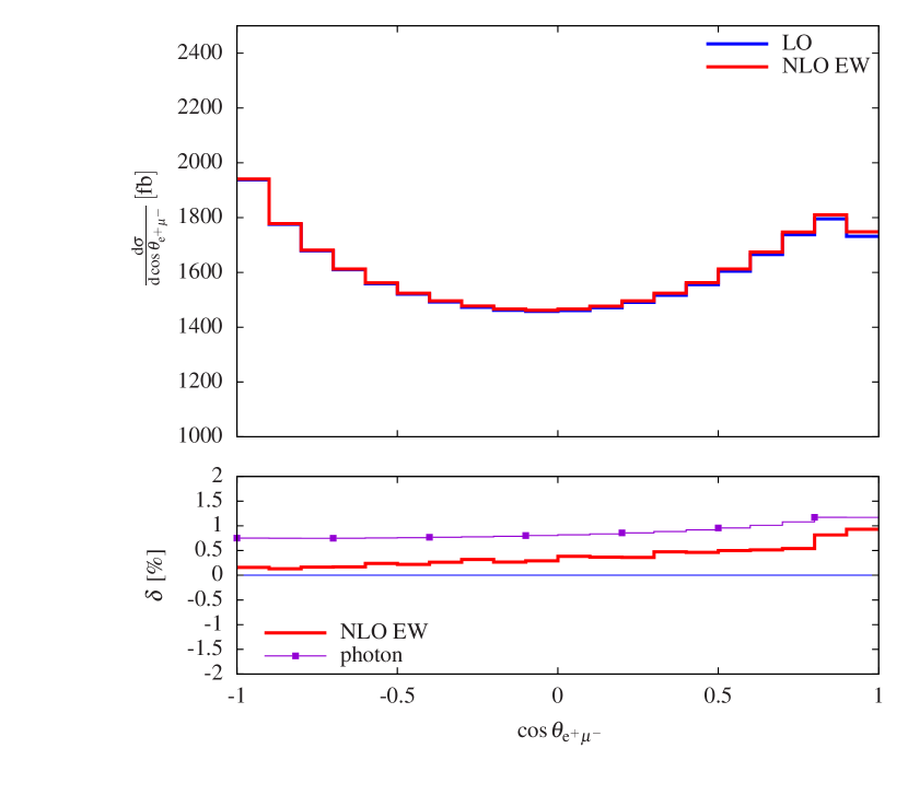
(c)

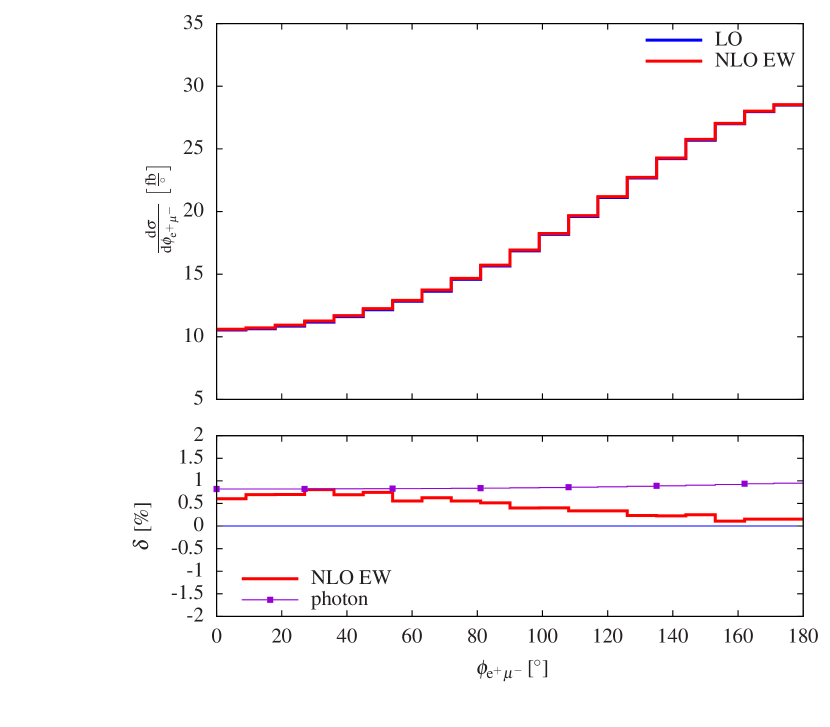
(d)

Figure 9: Differential distributions at a centre-of-mass energy $\sqrt{s}=13\,\text{TeV}$ at the LHC: the rapidity of the harder bottom quark 9(a) (upper left), the rapidity of the reconstructed top quark 9(b) (upper right), 9(c) the cosine of the angle between the positron and the muon (lower left), and 9(d) the azimuthal angle between the positron and the muon in the transverse plane (lower right). The lower panel shows the relative NLO EW correction $\delta=\sigma_{\text{NLO EW}}/\sigma_{\text{LO}}-1$ and the relative photon-induced contributions $\delta=\sigma_{\gamma g}/\sigma_{\text{LO}}$ in per cent.

The rapidity distributions of the harder bottom quark and the reconstructed top quark are shown in Figures 9(a) and 9(b), respectively. The rapidity distributions of the other final states exhibit flat EW corrections similar to the ones displayed in Figure 9(a). Over the whole rapidity range, the EW corrections are small and do not show any special features, while the photon-induced contributions are somewhat more important at high rapidities. This is particularly true for the rapidity distribution of the reconstructed top quark. There, the photon-induced contribution accounts for up to $3\%$ for large rapidities, i.e. for top quarks that have been produced close to the beam, while the EW corrections do not vary over the rapidity range considered here. The corrections for the distribution in the cosine of the angle between the two charged leptons (Figure 9(c)) and the distribution in the azimuthal angle in the transverse plane between them (Figure 9(d)) do not show particular features and are below $1\%$.

For the observables involving the reconstructed top quarks, we have found qualitative agreement with the results presented in Ref. Pagani:2016caq . Since the calculation of the complete corrections requires appropriate selection cuts to avoid IR singularities, no quantitative comparison of distributions is possible with existing calculations for on-shell top quarks.

3.4 Comparison to the double-pole approximation

We have studied two different DPAs for the off-shell production of top-quark pairs. The first one requires two resonant top quarks while the second one two resonant W bosons. In this section, we investigate the quality of these approximations by comparing them with the full calculation at the cross-section level as well as the differential-distribution level.

Integrated cross section

We first investigate the DPAs at LO and show results for the total LO cross section for both channels in Table 2. While the WW DPA is in agreement with the full LO result within one per cent, the tt DPA only agrees within $3\%$. This is the order of magnitude $\Gamma/M$ expected for a DPA. The better quality of the WW DPA results from the fact, that most diagrams for the full process and, in particular, those with two top resonances contain already two intermediate W bosons. On the other hand, there are much more diagrams involving only one or no resonant top quark.

Ch.	$\sigma^{\rm WW\;DPA}_{\rm LO}$ [fb]	$\delta^{\rm WW\;DPA}_{\rm LO}$ [$\%$]	$\sigma^{\rm tt\;DPA}_{\rm LO}$ [fb]	$\delta^{\rm tt\;DPA}_{\rm LO}$ [$\%$]
gg	$2808.4(6)$	$-0.56$	$2738.8(2)$	$-3.0$
${q\bar{q}}$	$372.90(1)$	$-0.64$	$368.82(1)$	$-2.2$
pp	$3181.3(5)$	$-0.57$	$3107.6(2)$	$-2.9$

Table 2: Integrated LO cross sections for the two DPAs. The relative difference is defined as $\delta^{\rm DPA}_{\rm LO}=\sigma^{\rm DPA}_{\rm LO}/\sigma^{\rm Full}_{\rm LO}-1$ in per cent.

At NLO, only the two channels that have been computed in the DPAs are shown in Table 3. Both approximations reproduce the total cross section within a per mille. We recall that the Born and real matrix elements have been computed with the full off-shell kinematics. This is also the case for the contributions involving the convolution operator ($P$ and $K$ operator in Ref. Catani:1996vz ), while the one arising from the $I$ operator has been evaluated with on-shell kinematics applied to the matrix element featuring two resonant propagators. As explained before the factorisable and non-factorisable virtual corrections have been computed within the DPA.

Ch.	$\sigma^{\rm WW\;DPA}_{\rm NLO\;EW}$ [fb]	$\delta^{\rm WW\;DPA}_{\rm NLO\;EW}$ [$\%$]	$\sigma^{\rm tt\;DPA}_{\rm NLO\;EW}$ [fb]	$\delta^{\rm tt\;DPA}_{\rm NLO\;EW}$ [$\%$]
gg	$2832.9(2)$	$-0.046$	$2836.5(2)$	$+0.082$
${q\bar{q}}$	$377.36(8)$	$0.047$	$377.23(5)$	$+0.013$
pp	$3210.5(2)$	$-0.037$	$3214.0(2)$	$+0.072$

Table 3: Integrated NLO cross section for the two DPAs. Only the channels where the DPAs are applied are shown. The relative difference is defined as $\delta^{\rm DPA}_{\rm NLO}=\sigma^{\rm DPA}_{\rm NLO}/\sigma^{\rm Full}_{\rm NLO}-1$ in per cent.

Differential distributions

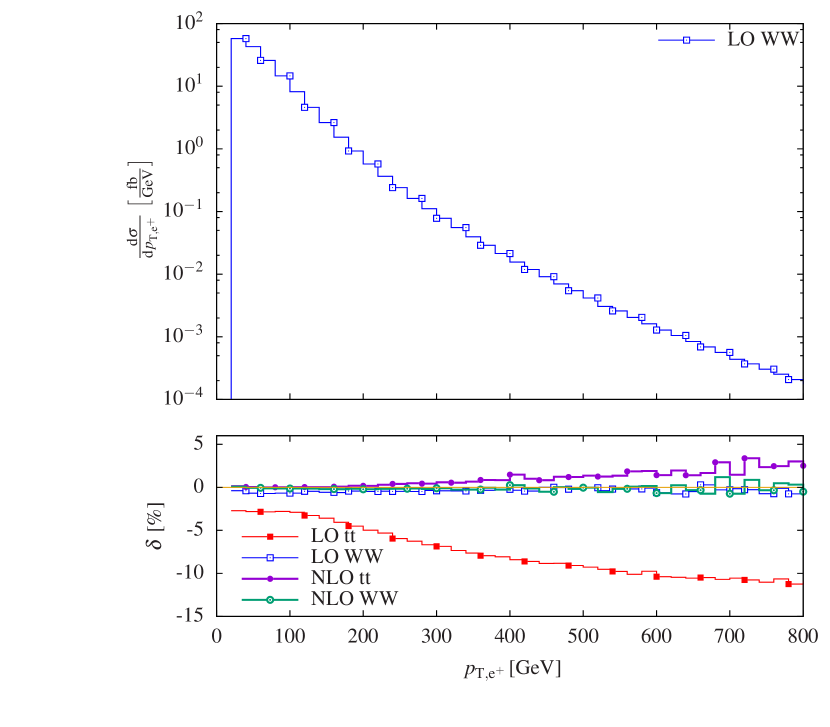
(a)

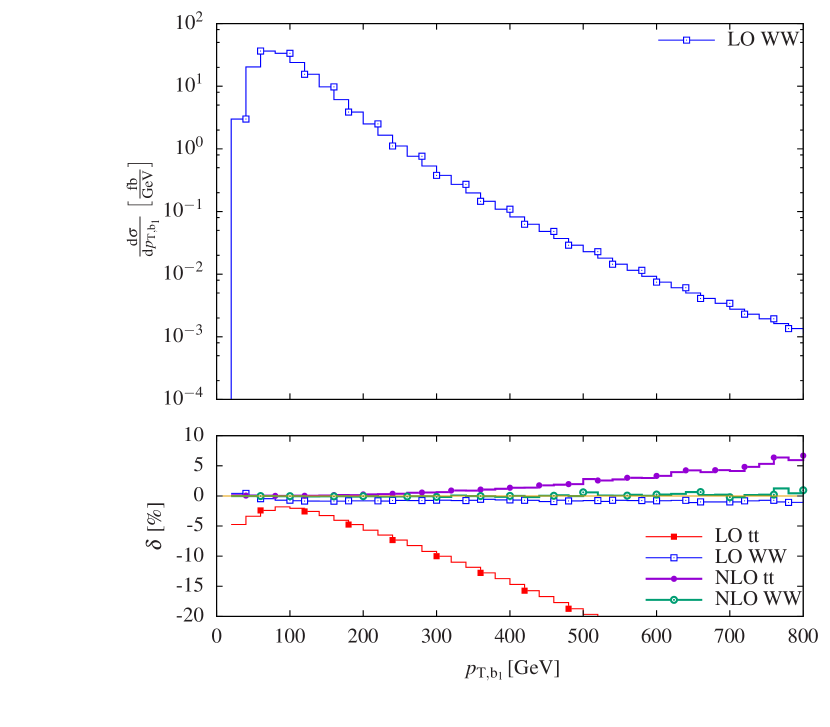
(b)

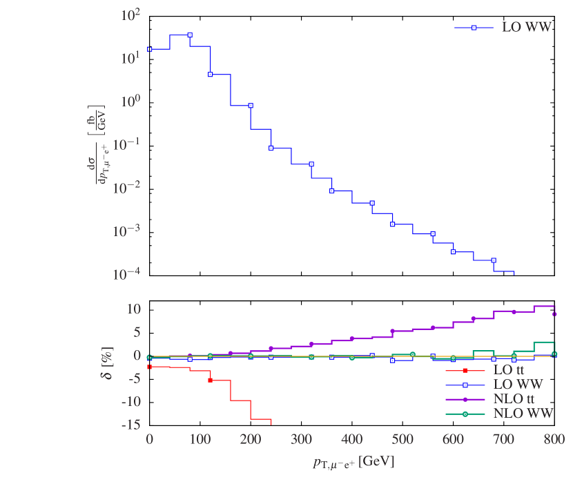
(c)

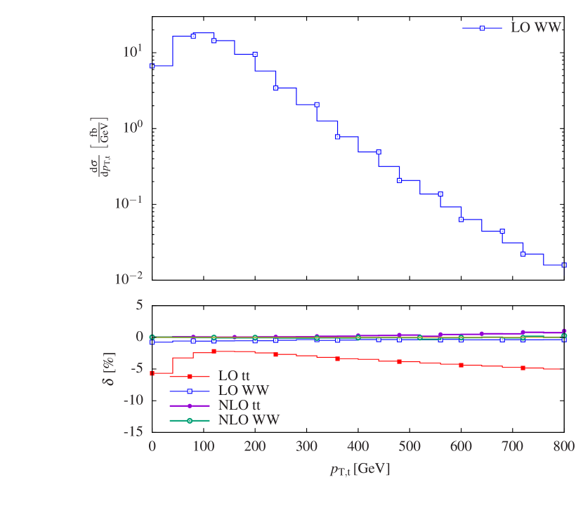
(d)

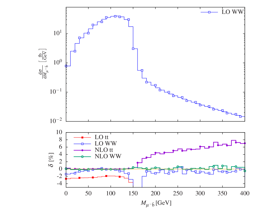
(e)

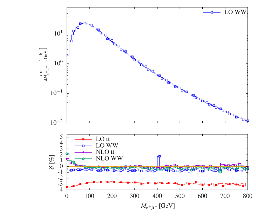
(f)

Figure 10: Comparison of full calculation and DPAs for various distributions at a centre-of-mass energy $\sqrt{s}=13\,\text{TeV}$ at the LHC: 10(a) transverse momentum for the positron (upper left), 10(b) transverse momentum for the harder b jet (upper right), 10(c) transverse momentum for the $\mu^{-}\text{e}^{+}$ system (middle left) 10(d) transverse momentum for reconstructed top quark (middle right), 10(e) invariant mass for the $\bar{\text{b}}\mu^{-}$ system (lower left), and 10(f) invariant mass for the $\text{e}^{+}\mu^{-}$ system (lower right). In the upper panel the LO distributions for the WW DPA are shown. The lower panel displays the relative deviation of the different DPAs from the full calculation, $\delta=\sigma_{\text{DPA}}/\sigma_{\text{Full}}-1$, in per cent.

A comparison of the full calculation with the two DPAs at the distribution level is presented in Figure 10. The upper panel contains only one curve (as on the logarithmic scale the three other curves are indistinguishable) which represents the WW DPA at LO. In the NLO computations, the DPA is not applied to the LO contributions, the real corrections, and to the $P$- and $K$-operator terms. In the lower panel, the differences between the approximations and the full calculation are displayed both at LO and NLO. The deviation with respect to the full calculation is defined as $\delta=\sigma_{\text{DPA}}/\sigma_{\text{Full}}-1$ and expressed in per cent.

The transverse momentum distributions of the electron (Figure 10(a)), of the harder bottom jet (Figure 10(b)), and of the $\text{e}^{+}\mu^{-}$ system (Figure 10(c)) display similar features at LO and NLO for both approximations. The WW DPA constitutes a better approximation than the tt one both at LO and NLO and agrees within $1\%$ for the observables studied in the considered phase space. The tt DPA, on the other hand, deviates by more than $30\%$ and $11\%$ at 800 GeV at LO and NLO, respectively.

In the transverse-momentum distributions of the positron and the harder bottom quark shown in Figures 10(a) and 10(b) the LO tt DPA deviates from the full leading order by more than $10\%$ and $20\%$, respectively, for transverse momenta above 500 GeV. This is due to the fact that it is easier to produce a particle with large transverse momentum directly than through an intermediate massive top quark. The effect is smaller for $p_{\mathrm{T},\text{e}^{+}}$ since there are only very few background diagrams where the positron does not result from the decay of a W boson. This effect is suppressed for the tt DPA at NLO, where the LO is treated exactly, but still leads to a disagreement of $3\%$ and $6\%$ for $p_{\mathrm{T},\text{e}^{+}}=800\,\text{GeV}$ and $p_{\mathrm{T},\text{b}_{1}}=800\,\text{GeV}$, respectively. On the other hand, the WW DPA approximation describes the full calculation within $1\%$ over the full kinematic range displayed.

The effects are even more dramatic for the distribution in the transverse momentum of the muon–positron system shown in Figure 10(c). The cross section is dominated by events where a pair of top quarks is produced with a back-to-back kinematics. For such events, the transverse momentum of a pair of decay products from different top quarks (for example the $\mu^{-}{\rm e}^{+}$ or the ${\rm b}\overline{{\rm b}}$ pair) tends to be small, and the high transverse-momentum region in these distributions receives sizeable corrections from contributions that do not result from the production of an on-shell top-quark pair. This explains the large discrepancy between the tt DPA and the full calculation that amounts to $11\%$ at NLO and more than $35\%$ at LO for $p_{\mathrm{T},\mu^{-}\text{e}^{+}}=800\,\text{GeV}$. The WW DPA, on the other hand, allows also contributions with only one or no resonant top quark and provides a good approximation also for this distribution.

We display in Figure 10(d), the distribution in the transverse momentum of the reconstructed top quark. There the two DPAs agree within $1\%$ with respect to the full calculation at NLO. At LO, the WW DPA works within $1\%$, while the tt DPA deviates by up to $5\%$, which is more or less within the expected accuracy of a pole approximation.

The invariant-mass distribution of the $\mu^{-}\bar{\text{b}}$ system in Figure 10(e) displays interesting features. Above the threshold at $M^{2}_{\rm t}-M^{2}_{\rm W}\simeq(154\,\text{GeV})^{2}$ the tt DPA is completely off at LO and only agrees within $10\%$ at NLO. This is due to the fact that this kinematical region is forbidden for on-shell top quarks and W bosons. Demanding only on-shell top quarks, the situation is quite similar as most off-shell W bosons are close to their mass shell. Requiring only on-shell W bosons, the top-quark invariant mass can become large and allows for a tail similar as for off-shell W bosons. This explains why almost no deviation from the full calculation is observed above the $M^{2}_{\rm t}-M^{2}_{\rm W}$ threshold for the WW DPA. The large differences of the WW DPA just above the threshold results from the fact that the approximation decreases faster than the full cross section owing to the broadening due to the W-boson width.

For the distribution in the invariant mass of the ${\rm\mu^{-}e^{+}}$ system, both approximations reproduce the full calculation at LO and NLO in shape well. The difference in the normalisation is as for the total cross-section (see Table 2).

Similarly, rapidity distributions do not show any shape deviation between neither of the two DPAs and the full calculation. The deviation in shape stays below one per cent for the distributions in the azimuthal-angle separation and the cosine of the angle between the two leptons.

To conclude, depending on the considered distribution the tt DPA does not always describe the full calculation properly. In some parts of phase space (especially in the high-energy limit) and for various distributions the disagreement can reach $10\%$. On the other hand, for all distributions that we have studied the WW DPA describes the full calculation within a per cent over the considered phase-space range. Note that we have specifically checked the transverse-momentum distribution of the $\text{e}^{+}\mu^{-}$ system (which is expected to be most sensitive to discrepancies between the WW DPA and full calculation) above 800 GeV and did not find larger deviations of the WW DPA from the full calculation. This can be explained by the fact that the WW DPA features all contributions with single or doubly top resonances and, thus, the neglected contributions are sub-dominant.

4 Conclusions

For the first time, the production of off-shell top-quark pairs including their leptonic decays has been computed at the NLO electroweak level. In this calculation, all off-shell, non-resonant, and interference effects have been taken into account. Moreover, the photon-induced channels have been evaluated for reference. The full NLO results have been supplemented by two different double-pole approximations, one assuming two resonant top quarks and one requiring two resonant W bosons.

We find electroweak corrections below one per cent for the integrated cross section, while the contribution from the photon-induced channel is at the per-cent level. For differential distributions the inclusion of electroweak corrections becomes particularly important as they can account for up to $15\%$ of the leading order. In this respect the photon-induced corrections have an effect opposite to the genuine electroweak corrections. While the electroweak corrections are negative in the high-energy limit due to the appearance of Sudakov logarithms, the photon-induced contributions are positive and increase with energy. Nonetheless, in the high-energy region the electroweak corrections become dominant and account for a significant decrease of the differential distributions.

We have found that the double-pole approximation requiring two resonant W bosons describes the full calculation satisfactorily in the considered phase-space regions. On the other hand, we observe sizeable discrepancies with respect to the full result for the double-pole approximation requiring two resonant top quarks in several distributions at both LO and NLO. This breakdown typically happens in distributions that involve the decay products of both the top and antitop quark. More precisely, differences appear in regions, where the contributions of two on-shell top quarks are suppressed. While such contributions are not taken into account in the top–antitop double-pole approximation, they are included in the WW one. We have found that the WW double-pole approximation constitutes a very good approximation of the full calculation for all the distributions that we have investigated. Nonetheless, it could fail for specific observables where off-shell W bosons play an important role. Thus, for arbitrary distributions over the whole phase space, one should only rely on the full calculation.

On the technical side, this calculation demonstrates the ability of the matrix-element generator Recola and of the integral library Collier to supply in an efficient and reliable way tree-level and one-loop amplitudes for complicated processes.

This study provides for the first time the electroweak corrections for a realistic off-shell production of top quark pairs at the LHC. It will help the experimental collaborations to measure the production of top-quark pairs to even higher precision at the LHC. Also, the higher-order corrections described in this article, as electroweak corrections in general, are relevant for the Standard Model background of new-physics searches. Indeed, they grow large exactly in the same phase-space region where one would expect new-physics contribution to appear, i.e. in the high-energy limit. Thus, our results will allow to test the Standard Model with better accuracy and help to discover new phenomena.

Appendix A Appendix

In this appendix we give the explicit expression of the $\Delta$s used in the computation of the non-factorisable corrections (12)–(14) expressed in terms of scalar integrals. We simply reproduce the formula of Ref. Dittmaier:2015bfe for completeness. The functions for the non-manifestly non-factorisable corrections read:

$$\Delta_{\mathrm{mm^{\prime}}}\left(i,j\right) {}\sim\begin{aligned} &-\left(\overline{\overline{s}}_{ij}-M^{2}_{i}-M^{2}_{j}\right)\bigg{\{}C_{0}\left(\overline{k}^{2}_{i},\overline{\overline{s}}_{ij},\overline{k}^{2}_{j},0,\overline{M}^{2}_{i},\overline{M}^{2}_{j}\right)\end{aligned}$$

$$\quad\begin{aligned} &-C_{0}\left({M}^{2}_{i},\overline{\overline{s}}_{ij},{M}^{2}_{j},m_{\gamma}^{2},{M}^{2}_{i},{M}^{2}_{j}\right)\bigg{\}},\end{aligned}$$ (28)

$$\Delta^{\prime}_{\mathrm{mm}}\left(i\right) {}\sim 2M_{i}^{2}\left\{\frac{B_{0}\left(\overline{k}^{2}_{i},0,\overline{M}^{2}_{i}\right)-B_{0}\left(\overline{M}^{2}_{i},m_{\gamma}^{2},\overline{M}^{2}_{i}\right)}{K_{i}}-B^{\prime}_{0}\left({M}^{2}_{i},m_{\gamma}^{2},{M}^{2}_{i}\right)\right\},$$ (29)

$$\Delta^{\prime}_{\mathrm{mf}}\left(i,a\right) {}\sim\begin{aligned} &-\left(\widetilde{s}_{ia}-M^{2}_{i}-m^{2}_{a}\right)\bigg{\{}C_{0}\left(\overline{k}^{2}_{i},{\widetilde{s}}_{ia},m_{a}^{2},0,\overline{M}^{2}_{i},m_{a}^{2}\right)\end{aligned}$$

$$\quad\begin{aligned} &-C_{0}\left(M^{2}_{i},{\widetilde{s}}_{ia},m_{a}^{2},m^{2}_{\gamma},{M}^{2}_{i},m_{a}^{2}\right)\bigg{\}},\end{aligned}$$ (30)

$$\Delta_{\mathrm{xm}}\left(i;b\right) {}\sim\begin{aligned} &-\left(\overline{s}_{ia}-M^{2}_{i}-m^{2}_{b}\right)\bigg{\{}C_{0}\left(\overline{k}^{2}_{i},{\overline{s}}_{ib},m_{b}^{2},0,\overline{M}^{2}_{i},m_{b}^{2}\right)\end{aligned}$$

$$\quad\begin{aligned} &-C_{0}\left(M^{2}_{i},{\overline{s}}_{ib},m_{b}^{2},m^{2}_{\gamma},{M}^{2}_{i},m_{b}^{2}\right)\bigg{\}}.\end{aligned}$$ (31)

The $\sim$ sign implies that the on-shell limit is taken everywhere where possible. This means that all quantities are evaluated with on-shell kinematics, while only the momenta of the resonant particles are kept off the mass shell. Note that each contribution consists of a scalar integral calculated with complex masses of the resonances subtracted with the corresponding integral for real masses but with a photon mass to regularise the IR singularities. While the IR singularities of the subtracted parts cancel exactly the matching contributions in the factorisable corrections, those in the original expressions appear as logarithms of the off-shell propagators and cancel implicitly upon adding the real corrections.

Finally, the functions for the manifestly non-factorisable virtual corrections read:

$$\Delta_{\mathrm{ff^{\prime}}}\left(i,a;j,b\right) \sim\begin{aligned} &-\left(s_{ab}-m^{2}_{a}-m^{2}_{b}\right)K_{i}K_{j}E_{0}\left(k_{a},\overline{k}_{i},-\overline{k}_{j},-{k}_{b},m_{\gamma}^{2},m_{a}^{2},\overline{M}^{2}_{i},\overline{M}^{2}_{j},m_{b}^{2}\right)\end{aligned}$$

$$\sim\begin{aligned} &-\left(s_{ab}-m^{2}_{a}-m^{2}_{b}\right)K_{i}K_{j}\\ &\times E_{0}\left(k^{2}_{a},\widetilde{s}_{ia},\overline{\overline{s}}_{ij},\widetilde{s}_{jb},k^{2}_{b},\overline{k}^{2}_{i},\overline{s}_{ja},\overline{s}_{ib},\overline{k}^{2}_{j},s_{ab},m_{\gamma}^{2},m_{a}^{2},\overline{M}^{2}_{i},\overline{M}^{2}_{j},m_{b}^{2}\right),\end{aligned}$$

$$\Delta^{\prime}_{\mathrm{mf^{\prime}}}\left(i;j,b\right) \sim\begin{aligned} &-\left(\overline{s}_{ib}-M_{i}^{2}-m^{2}_{b}\right)K_{j}D_{0}\left(\overline{k}_{i},-\overline{k}_{j},-{k}_{b},m_{\gamma}^{2},\overline{M}^{2}_{i},\overline{M}^{2}_{j},m_{b}^{2}\right)\end{aligned}$$

$$\sim\begin{aligned} &-\left(\overline{s}_{ib}-M_{i}^{2}-m^{2}_{b}\right)K_{j}D_{0}\left(\overline{k}^{2}_{i},\overline{\overline{s}}_{ij},\widetilde{s}_{jb},k^{2}_{b},\overline{k}^{2}_{j},\overline{s}_{ib},m_{\gamma}^{2},\overline{M}^{2}_{i},\overline{M}^{2}_{j},m_{b}^{2}\right),\end{aligned}$$ (33)

$$\Delta_{\mathrm{xf}}\left(i,a;b\right) \sim\begin{aligned} &-\left(s_{ab}-m^{2}_{a}-m^{2}_{b}\right)K_{i}D_{0}\left({k}_{a},\overline{k}_{i},-{k}_{b},m_{\gamma}^{2},m_{a}^{2},\overline{M}^{2}_{i},m_{b}^{2}\right)\end{aligned}$$

$$\sim\begin{aligned} &-\left(s_{ab}-m^{2}_{a}-m^{2}_{b}\right)K_{i}D_{0}\left({k}^{2}_{a},\widetilde{s}_{ia},\overline{s}_{ib},k^{2}_{b},\overline{k}_{i}^{2},s_{ab},m_{\gamma}^{2},m_{a}^{2},\overline{M}^{2}_{i},m_{b}^{2}\right),\end{aligned}$$ (34)

where the arguments of the scalar integrals have been rewritten in terms of invariants. The identification with scalar integrals in terms of momentum arguments reads:

$$D_{0}\left(p_{1},p_{2},p_{3},m_{\gamma}^{2},m_{1}^{2},m_{2}^{2},m_{3}^{2}\right)\equiv\\ D_{0}\left(p_{1}^{2},\left(p_{2}-p_{1}\right)^{2},\left(p_{3}-p_{2}\right)^{2},p^{2}_{3},p^{2}_{2},\left(p_{3}-p_{1}\right)^{2},m_{\gamma}^{2},m_{1}^{2},m_{2}^{2},m_{3}^{2}\right),$$ (35)

and

$$E_{0}\left(p_{1},p_{2},p_{3},p_{4},m_{\gamma}^{2},m_{1}^{2},m_{2}^{2},m_{3}^{2},m_{4}^{2}\right)\equiv\\ E_{0}\big{(}p_{1}^{2},\left(p_{2}-p_{1}\right)^{2},\left(p_{3}-p_{2}\right)^{2},\left(p_{4}-p_{3}\right)^{2},p^{2}_{4},p^{2}_{2},\\ \left(p_{3}-p_{1}\right)^{2},\left(p_{4}-p_{2}\right)^{2},p^{2}_{3},\left(p_{4}-p_{1}\right)^{2},m_{\gamma}^{2},m_{1}^{2},m_{2}^{2},m_{3}^{2},m_{4}^{2}\big{)}.$$ (36)

The scalar integrals used for the numerical evaluation have been obtained from the Collier library Denner:2014gla ; Denner:2016kdg .

References

- (1) CMS Collaboration, S. Chatrchyan et al., Measurement of the production cross section in the dilepton channel in collisions at 7 TeV, JHEP 11 (2012) 067, [arXiv:1208.2671].
- (2) CMS Collaboration, S. Chatrchyan et al., Measurement of the production cross section in the dilepton channel in pp collisions at = 8 TeV, JHEP 02 (2014) 024, [arXiv:1312.7582]. [Erratum: JHEP 02 (2014) 102].
- (3) ATLAS Collaboration, G. Aad et al., Measurement of the production cross-section using events with -tagged jets in collisions at 7 and 8 TeV with the ATLAS detector, Eur. Phys. J. C74 (2014) 3109, [arXiv:1406.5375].
- (4) CMS Collaboration, V. Khachatryan et al., Measurement of the top quark pair production cross section in proton-proton collisions at 13 TeV, Phys. Rev. Lett. 116 (2016) 052002, [arXiv:1510.05302].
- (5) V. del Duca and E. Laenen, Top physics at the LHC, Int. J. Mod. Phys. A30 (2015) 1530063, [arXiv:1510.06690].
- (6) ATLAS Collaboration, M. Aaboud et al., Measurement of the production cross-section using events with b-tagged jets in pp collisions at 13 TeV with the ATLAS detector, arXiv:1606.02699.
- (7) P. Nason, S. Dawson, and R. K. Ellis, The one particle inclusive differential cross-section for heavy quark production in hadronic collisions, Nucl. Phys. B327 (1989) 49–92. [Erratum: Nucl. Phys. B335 (1990) 260].
- (8) W. Beenakker, W. L. van Neerven, R. Meng, G. A. Schuler, and J. Smith, QCD corrections to heavy quark production in hadron hadron collisions, Nucl. Phys. B351 (1991) 507–560.
- (9) M. L. Mangano, P. Nason, and G. Ridolfi, Heavy quark correlations in hadron collisions at next-to-leading order, Nucl. Phys. B373 (1992) 295–345.
- (10) S. Frixione, M. L. Mangano, P. Nason, and G. Ridolfi, Top quark distributions in hadronic collisions, Phys. Lett. B351 (1995) 555–561, [hep-ph/9503213].
- (11) W. Bernreuther, A. Brandenburg, Z. G. Si, and P. Uwer, Top quark pair production and decay at hadron colliders, Nucl. Phys. B690 (2004) 81–137, [hep-ph/0403035].
- (12) K. Melnikov and M. Schulze, NLO QCD corrections to top quark pair production and decay at hadron colliders, JHEP 08 (2009) 049, [arXiv:0907.3090].
- (13) W. Bernreuther and Z.-G. Si, Distributions and correlations for top quark pair production and decay at the Tevatron and LHC, Nucl. Phys. B837 (2010) 90–121, [arXiv:1003.3926].
- (14) J. M. Campbell and R. K. Ellis, Top-quark processes at NLO in production and decay, J. Phys. G42 (2015) 015005, [arXiv:1204.1513].
- (15) A. Denner, S. Dittmaier, S. Kallweit, and S. Pozzorini, NLO QCD corrections to WWbb production at hadron colliders, Phys. Rev. Lett. 106 (2011) 052001, [arXiv:1012.3975].
- (16) G. Bevilacqua, M. Czakon, A. van Hameren, C. G. Papadopoulos, and M. Worek, Complete off-shell effects in top quark pair hadroproduction with leptonic decay at next-to-leading order, JHEP 02 (2011) 083, [arXiv:1012.4230].
- (17) A. Denner, S. Dittmaier, S. Kallweit, and S. Pozzorini, NLO QCD corrections to off-shell top-antitop production with leptonic decays at hadron colliders, JHEP 10 (2012) 110, [arXiv:1207.5018].
- (18) R. Frederix, Top quark induced backgrounds to Higgs production in the decay channel at NLO in QCD, Phys. Rev. Lett. 112 (2014) 082002, [arXiv:1311.4893].
- (19) S. Frixione, P. Nason, and B. R. Webber, Matching NLO QCD and parton showers in heavy flavor production, JHEP 08 (2003) 007, [hep-ph/0305252].
- (20) S. Frixione, P. Nason, and G. Ridolfi, A positive-weight next-to-leading-order Monte Carlo for heavy flavour hadroproduction, JHEP 09 (2007) 126, [arXiv:0707.3088].
- (21) S. Höche, et al., Next-to-leading order QCD predictions for top-quark pair production with up to two jets merged with a parton shower, Phys. Lett. B748 (2015) 74–78, [arXiv:1402.6293].
- (22) M. V. Garzelli, A. Kardos, and Z. Trócsanyi, Hadroproduction of at NLO accuracy matched with shower Monte Carlo programs, JHEP 08 (2014) 069, [arXiv:1405.5859].
- (23) J. M. Campbell, R. K. Ellis, P. Nason, and E. Re, Top-pair production and decay at NLO matched with parton showers, JHEP 04 (2015) 114, [arXiv:1412.1828].
- (24) T. Ježo, J. M. Lindert, P. Nason, C. Oleari, and S. Pozzorini, An NLO+PS generator for and production and decay including non-resonant and interference effects, arXiv:1607.04538.
- (25) M. Czakon, P. Fiedler, and A. Mitov, Total top-quark pair-production cross section at hadron colliders through , Phys. Rev. Lett. 110 (2013) 252004, [arXiv:1303.6254].
- (26) M. Czakon, P. Fiedler, D. Heymes, and A. Mitov, NNLO QCD predictions for fully-differential top-quark pair production at the Tevatron, arXiv:1601.05375.
- (27) M. Czakon, D. Heymes, and A. Mitov, Dynamical scales for multi-TeV top-pair production at the LHC, arXiv:1606.03350.
- (28) M. Beneke, P. Falgari, and C. Schwinn, Soft radiation in heavy-particle pair production: All-order colour structure and two-loop anomalous dimension, Nucl. Phys. B828 (2010) 69–101, [arXiv:0907.1443].
- (29) M. Czakon, A. Mitov, and G. F. Sterman, Threshold resummation for top-pair hadroproduction to next-to-next-to-leading log, Phys. Rev. D80 (2009) 074017, [arXiv:0907.1790].
- (30) V. Ahrens, A. Ferroglia, M. Neubert, B. D. Pecjak, and L. L. Yang, Renormalization-group improved predictions for top-quark pair production at hadron colliders, JHEP 09 (2010) 097, [arXiv:1003.5827].
- (31) N. Kidonakis, Two-loop soft anomalous dimensions and NNLL resummation for heavy quark production, Phys. Rev. Lett. 102 (2009) 232003, [arXiv:0903.2561].
- (32) N. Kidonakis, Next-to-next-to-leading soft-gluon corrections for the top quark cross section and transverse momentum distribution, Phys. Rev. D82 (2010) 114030, [arXiv:1009.4935].
- (33) W. Beenakker, et al., Electroweak one-loop contributions to top pair production in hadron colliders, Nucl. Phys. B411 (1994) 343–380.
- (34) W. Bernreuther, M. Fücker, and Z. G. Si, Mixed QCD and weak corrections to top quark pair production at hadron colliders, Phys. Lett. B633 (2006) 54–60, [hep-ph/0508091]. [Erratum: Phys. Lett. B644 (2007) 386].
- (35) J. H. Kühn, A. Scharf, and P. Uwer, Electroweak corrections to top-quark pair production in quark-antiquark annihilation, Eur. Phys. J. C45 (2006) 139–150, [hep-ph/0508092].
- (36) S. Moretti, M. R. Nolten, and D. A. Ross, Weak corrections to gluon-induced top-antitop hadro-production, Phys. Lett. B639 (2006) 513–519, [hep-ph/0603083]. [Erratum: Phys. Lett. B660 (2008) 607].
- (37) J. H. Kühn, A. Scharf, and P. Uwer, Electroweak effects in top-quark pair production at hadron colliders, Eur. Phys. J. C51 (2007) 37–53, [hep-ph/0610335].
- (38) W. Bernreuther, M. Fücker, and Z.-G. Si, Weak interaction corrections to hadronic top quark pair production, Phys. Rev. D74 (2006) 113005, [hep-ph/0610334].
- (39) W. Hollik and M. Kollar, NLO QED contributions to top-pair production at hadron collider, Phys. Rev. D77 (2008) 014008, [arXiv:0708.1697].
- (40) W. Bernreuther, M. Fücker, and Z.-G. Si, Electroweak corrections to production at hadron colliders, Nuovo Cim. B123 (2008) 1036–1044, [arXiv:0808.1142].
- (41) W. Bernreuther, M. Fücker, and Z.-G. Si, Weak interaction corrections to hadronic top quark pair production: contributions from quark-gluon and induced reactions, Phys. Rev. D78 (2008) 017503, [arXiv:0804.1237].
- (42) M. Beneke, A. Maier, J. Piclum, and T. Rauh, Higgs effects in top anti-top production near threshold in annihilation, Nucl. Phys. B899 (2015) 180–193, [arXiv:1506.06865].
- (43) D. Pagani, I. Tsinikos, and M. Zaro, The impact of the photon PDF and electroweak corrections on distributions, arXiv:1606.01915.
- (44) R. Frederix and F. Maltoni, Top pair invariant mass distribution: A window on new physics, JHEP 01 (2009) 047, [arXiv:0712.2355].
- (45) W. Bernreuther, P. Galler, C. Mellein, Z. G. Si, and P. Uwer, Production of heavy Higgs bosons and decay into top quarks at the LHC, Phys. Rev. D93 (2016) 034032, [arXiv:1511.05584].
- (46) N. Greiner, K. Kong, J.-C. Park, S. C. Park, and J.-C. Winter, Model-independent production of a top-philic resonance at the LHC, JHEP 04 (2015) 029, [arXiv:1410.6099].
- (47) M. Backovic, et al., Higher-order QCD predictions for dark matter production at the LHC in simplified models with s-channel mediators, Eur. Phys. J. C75 (2015) 482, [arXiv:1508.05327].
- (48) C. Arina, et al., A comprehensive approach to dark matter studies: exploration of simplified top-philic models, arXiv:1605.09242.
- (49) B. Hespel, F. Maltoni, and E. Vryonidou, Signal background interference effects in heavy scalar production and decay to a top-anti-top pair, arXiv:1606.04149.
- (50) A. Denner, S. Dittmaier, M. Roth, and D. Wackeroth, Electroweak radiative corrections to 4 fermions in double pole approximation: The RACOONWW approach, Nucl. Phys. B587 (2000) 67–117, [hep-ph/0006307].
- (51) E. Accomando, A. Denner, and A. Kaiser, Logarithmic electroweak corrections to gauge-boson pair production at the LHC, Nucl. Phys. B706 (2005) 325–371, [hep-ph/0409247].
- (52) D. Wackeroth and W. Hollik, Electroweak radiative corrections to resonant charged gauge boson production, Phys. Rev. D55 (1997) 6788–6818, [hep-ph/9606398].
- (53) U. Baur, S. Keller, and D. Wackeroth, Electroweak radiative corrections to -boson production in hadronic collisions, Phys. Rev. D59 (1999) 013002, [hep-ph/9807417].
- (54) S. Dittmaier and M. Krämer, Electroweak radiative corrections to W-boson production at hadron colliders, Phys. Rev. D65 (2002) 073007, [hep-ph/0109062].
- (55) S. Jadach, W. Placzek, M. Skrzypek, B. F. L. Ward, and Z. Was, Exact gauge invariant YFS exponentiated Monte Carlo for (un)stable production at and beyond LEP2 energies, Phys. Lett. B417 (1998) 326–336, [hep-ph/9705429].
- (56) A. Denner, S. Dittmaier, and M. Roth, Nonfactorizable photonic corrections to 4 fermions, Nucl. Phys. B519 (1998) 39–84, [hep-ph/9710521].
- (57) S. Jadach, W. Placzek, M. Skrzypek, B. F. L. Ward, and Z. Was, Final state radiative effects for the exact YFS exponentiated (un)stable production at and beyond LEP2 energies, Phys. Rev. D61 (2000) 113010, [hep-ph/9907436].
- (58) W. Beenakker, F. A. Berends, and A. P. Chapovsky, Radiative corrections to pair production of unstable particles: results for 4 fermions, Nucl. Phys. B548 (1999) 3–59, [hep-ph/9811481].
- (59) A. P. Chapovsky and V. A. Khoze, Screened-Coulomb ansatz for the non-factorizable radiative corrections to the off-shell production, Eur. Phys. J. C9 (1999) 449–457, [hep-ph/9902343].
- (60) A. Bredenstein, S. Dittmaier, and M. Roth, Four-fermion production at colliders. 2. Radiative corrections in double-pole approximation, Eur. Phys. J. C44 (2005) 27–49, [hep-ph/0506005].
- (61) M. Billoni, S. Dittmaier, B. Jäger, and C. Speckner, Next-to-leading order electroweak corrections to pp 4 leptons at the LHC in double-pole approximation, JHEP 12 (2013) 043, [arXiv:1310.1564].
- (62) S. Dittmaier and C. Schwan, Non-factorizable photonic corrections to resonant production and decay of many unstable particles, Eur. Phys. J. C76 (2016) 144, [arXiv:1511.01698].
- (63) R. Feger, “MoCaNLO: a generic Monte Carlo event generator for NLO calculations of hadron-collider processes.” unpublished, 2015.
- (64) S. Actis, A. Denner, L. Hofer, A. Scharf, and S. Uccirati, Recursive generation of one-loop amplitudes in the Standard Model, JHEP 04 (2013) 037, [arXiv:1211.6316].
- (65) S. Actis, et al., RECOLA: REcursive Computation of One-Loop Amplitudes, arXiv:1605.01090.
- (66) A. Denner and R. Feger, NLO QCD corrections to off-shell top-antitop production with leptonic decays in association with a Higgs boson at the LHC, JHEP 11 (2015) 209, [arXiv:1506.07448].
- (67) G. Bevilacqua, H. B. Hartanto, M. Kraus, and M. Worek, Top quark pair production in association with a jet with next-to-leading-order QCD off-shell effects at the Large Hadron Collider, Phys. Rev. Lett. 116 (2016) 052003, [arXiv:1509.09242].
- (68) S. Kallweit, J. M. Lindert, P. Maierhöfer, S. Pozzorini, and M. Schönherr, NLO QCD+EW predictions for V + jets including off-shell vector-boson decays and multijet merging, JHEP 04 (2016) 021, [arXiv:1511.08692].
- (69) F. F. Cordero, P. Hofmann, and H. Ita, + 3 jet production at the Large Hadron Collider in NLO QCD, arXiv:1512.07591.
- (70) B. Biedermann, A. Denner, S. Dittmaier, L. Hofer, and B. Jäger, Electroweak corrections to at the LHC: a Higgs background study, Phys. Rev. Lett. 116 (2016) 161803, [arXiv:1601.07787].
- (71) B. Biedermann, et al., Next-to-leading-order electroweak corrections to leptons at the LHC, JHEP 06 (2016) 065, [arXiv:1605.03419].
- (72) F. A. Berends, R. Pittau, and R. Kleiss, All electroweak four fermion processes in electron-positron collisions, Nucl. Phys. B424 (1994) 308–342, [hep-ph/9404313].
- (73) A. Denner, S. Dittmaier, M. Roth, and D. Wackeroth, Predictions for all processes 4 fermions , Nucl. Phys. B560 (1999) 33–65, [hep-ph/9904472].
- (74) S. Dittmaier and M. Roth, LUSIFER: A LUcid approach to six FERmion production, Nucl. Phys. B642 (2002) 307–343, [hep-ph/0206070].
- (75) S. Catani and M. H. Seymour, A general algorithm for calculating jet cross-sections in NLO QCD, Nucl. Phys. B485 (1997) 291–419, [hep-ph/9605323]. [Erratum: Nucl. Phys. B510 (1998) 503].
- (76) S. Dittmaier, A general approach to photon radiation off fermions, Nucl. Phys. B565 (2000) 69–122, [hep-ph/9904440].
- (77) S. Catani, S. Dittmaier, M. H. Seymour, and Z. Trocsanyi, The dipole formalism for next-to-leading order QCD calculations with massive partons, Nucl. Phys. B627 (2002) 189–265, [hep-ph/0201036].
- (78) L. Phaf and S. Weinzierl, Dipole formalism with heavy fermions, JHEP 04 (2001) 006, [hep-ph/0102207].
- (79) A. Denner, S. Dittmaier, and L. Hofer, Collier - A fortran-library for one-loop integrals, PoS LL2014 (2014) 071, [arXiv:1407.0087].
- (80) A. Denner, S. Dittmaier, and L. Hofer, Collier: a fortran-based Complex One-Loop LIbrary in Extended Regularizations, arXiv:1604.06792.
- (81) NNPDF Collaboration, R. D. Ball, et al., Parton distributions with QED corrections, Nucl. Phys. B877 (2013) 290–320, [arXiv:1308.0598].
- (82) K. P. O. Diener, S. Dittmaier, and W. Hollik, Electroweak higher-order effects and theoretical uncertainties in deep-inelastic neutrino scattering, Phys. Rev. D72 (2005) 093002, [hep-ph/0509084].
- (83) S. Dittmaier and M. Huber, Radiative corrections to the neutral-current Drell-Yan process in the Standard Model and its minimal supersymmetric extension, JHEP 01 (2010) 060, [arXiv:0911.2329].
- (84) G. ’t Hooft and M. J. G. Veltman, Scalar one loop integrals, Nucl. Phys. B153 (1979) 365–401.
- (85) W. Beenakker and A. Denner, Infrared divergent scalar box integrals with applications in the electroweak Standard Model, Nucl. Phys. B338 (1990) 349–370.
- (86) S. Dittmaier, Separation of soft and collinear singularities from one-loop N point integrals, Nucl. Phys. B675 (2003) 447–466, [hep-ph/0308246].
- (87) A. Denner and S. Dittmaier, Scalar one-loop 4-point integrals, Nucl. Phys. B844 (2011) 199–242, [arXiv:1005.2076].
- (88) G. Passarino and M. J. G. Veltman, One-loop corrections for annihilation into in the Weinberg Model, Nucl. Phys. B160 (1979) 151.
- (89) A. Denner and S. Dittmaier, Reduction of one-loop tensor 5-point integrals, Nucl. Phys. B658 (2003) 175–202, [hep-ph/0212259].
- (90) A. Denner and S. Dittmaier, Reduction schemes for one-loop tensor integrals, Nucl. Phys. B734 (2006) 62–115, [hep-ph/0509141].
- (91) A. Denner, S. Dittmaier, M. Roth, and L. H. Wieders, Electroweak corrections to charged-current 4 fermion processes: Technical details and further results, Nucl. Phys. B724 (2005) 247–294, [hep-ph/0505042]. [Erratum: Nucl. Phys. B854 (2012) 504].
- (92) A. Denner and S. Dittmaier, The complex-mass scheme for perturbative calculations with unstable particles, Nucl. Phys. Proc. Suppl. 160 (2006) 22–26, [hep-ph/0605312].
- (93) V. S. Fadin, V. A. Khoze, and A. D. Martin, How suppressed are the radiative interference effects in heavy instable particle production?, Phys. Lett. B320 (1994) 141–144, [hep-ph/9309234].
- (94) V. S. Fadin, V. A. Khoze, and A. D. Martin, Interference radiative phenomena in the production of heavy unstable particles, Phys. Rev. D49 (1994) 2247–2256.
- (95) K. Melnikov and O. I. Yakovlev, Top near threshold: all corrections are trivial, Phys. Lett. B324 (1994) 217–223, [hep-ph/9302311].
- (96) R. G. Stuart, Gauge invariance, analyticity and physical observables at the Z0 resonance, Phys. Lett. B262 (1991) 113–119.
- (97) H. G. J. Veltman, Mass and width of unstable gauge bosons, Z. Phys. C62 (1994) 35–52.
- (98) A. Aeppli, F. Cuypers, and G. J. van Oldenborgh, corrections to W pair production in and collisions, Phys. Lett. B314 (1993) 413–420, [hep-ph/9303236].
- (99) W. Beenakker, A. P. Chapovsky, and F. A. Berends, Non-factorizable corrections to W-pair production: Methods and analytic results, Nucl. Phys. B508 (1997) 17–63, [hep-ph/9707326].
- (100) A. Denner, R. Feger, and A. Scharf, Irreducible background and interference effects for Higgs-boson production in association with a top-quark pair, JHEP 04 (2015) 008, [arXiv:1412.5290].
- (101) J. Alwall, et al., The automated computation of tree-level and next-to-leading order differential cross sections, and their matching to parton shower simulations, JHEP 07 (2014) 079, [arXiv:1405.0301].
- (102) Z. Nagy and Z. Trocsanyi, Next-to-leading order calculation of four-jet observables in electron-positron annihilation, Phys. Rev. D59 (1999) 014020, [hep-ph/9806317]. [Erratum: Phys. Rev. D62 (2000) 099902].
- (103) J. R. Andersen et al., Les Houches 2013: Physics at TeV Colliders: Standard Model Working Group Report, arXiv:1405.1067.
- (104) A. Buckley, et al., LHAPDF6: parton density access in the LHC precision era, Eur. Phys. J. C75 (2015) 132, [arXiv:1412.7420].
- (105) NNPDF Collaboration, S. Carrazza, Towards the determination of the photon parton distribution function constrained by LHC data, PoS DIS2013 (2013) 279, [arXiv:1307.1131].
- (106) NNPDF Collaboration, S. Carrazza, Towards an unbiased determination of parton distributions with QED corrections, in Proceedings, 48th Rencontres de Moriond on QCD and High Energy Interactions, pp. 357–360, 2013. arXiv:1305.4179.
- (107) F. Demartin, S. Forte, E. Mariani, J. Rojo, and A. Vicini, The impact of PDF and uncertainties on Higgs Production in gluon fusion at hadron colliders, Phys. Rev. D82 (2010) 014002, [arXiv:1004.0962].
- (108) Particle Data Group Collaboration, J. Beringer et al., Review of Particle Physics (RPP), Phys. Rev. D86 (2012) 010001.
- (109) L. Basso, S. Dittmaier, A. Huss, and L. Oggero, Techniques for the treatment of IR divergences in decay processes at NLO and application to the top-quark decay, arXiv:1507.04676.
- (110) M. Jezabek and J. H. Kühn, QCD corrections to semileptonic decays of heavy quarks, Nucl. Phys. B314 (1989) 1.
- (111) D. Yu. Bardin, A. Leike, T. Riemann, and M. Sachwitz, Energy-dependent width effects in -annihilation near the Z-boson pole, Phys. Lett. B206 (1988) 539–542.
- (112) M. Cacciari, G. P. Salam, and G. Soyez, The anti- jet clustering algorithm, JHEP 04 (2008) 063, [arXiv:0802.1189].