Smoothing the payoff for efficient computation of Basket option prices

Abstract.

We consider the problem of pricing basket options in a multivariate Black-Scholes or Variance-Gamma model. From a numerical point of view, pricing such options corresponds to moderate and high-dimensional numerical integration problems with non-smooth integrands. Due to this lack of regularity, higher order numerical integration techniques may not be directly available, requiring the use of methods like Monte Carlo specifically designed to work for non-regular problems. We propose to use the inherent smoothing property of the density of the underlying in the above models to mollify the payoff function by means of an exact conditional expectation. The resulting conditional expectation is unbiased and yields a smooth integrand, which is amenable to the efficient use of adaptive sparse-grid cubature. Numerical examples indicate that the high-order method may perform orders of magnitude faster than Monte Carlo or Quasi Monte Carlo methods in dimensions up to $35$.

1. Introduction

In quantitative finance, the price of an option on an underlying $S$ can typically—disregarding discounting—be expressed as $E[f(S)]$ for some (payoff) function $f$ on $S$ and the expectation operator $E$ induced by the appropriate pricing measure. Hence, option pricing is an integration problem. The integration problem is usually challenging due to a combination of two complications:

• $S$ often takes values in a high-dimensional space. The reason for the high dimensionality may be time discretization of a stochastic differential equation, path dependence of the option (i.e., $S$ is actually a path of an asset price, not the value at a specific time), a large number of underlying assets, or others.

• the payoff function $f$ is typically not smooth.

In this work, we focus on the problem of pricing basket options in models, where the distribution of the underlying is explicitly given to us. Specifically, we consider multivariate Black-Scholes and Variance-Gamma models, i.e., models, for which no time discretization is required. We consider a basket option on a $d$-dimensional underlying asset $S_{T}=\left(S^{1}_{T},\ldots,S^{d}_{T}\right)$ with payoff function

$$f(S_{T})=\left(\sum_{i=1}^{d}w_{i}S^{i}_{T}-K\right)^{+}$$

for some positive weights $w_{1},\ldots,w_{d}$, a maturity $T$ and a strike price $K$. Observe in passing that one could also allow some weights to be negative, an option type known as “spread option”. Note that in addition, (discrete) Asian options also fall under this framework.

Even in the standard Black-Scholes framework, closed-form expressions for basket option prices are not available, since sums of log-normal random variables are generally not log-normally distributed. Some explicit approximation formulas are based on approximate distributional identities of sums of log-normal random variables; for instance, see [12, 26]. In addition, Laplace’s method, possibly coupled with heat kernel expansions when the distribution of the factors $S^{i}_{T}$ are given only as solutions of stochastic differential equations, has been shown to yield highly exact results even in high dimensions ([5, 4, 6]). In this work, however, we aim to solve the problem at hand using generic numerical integration techniques, which remain available beyond the restrictions of the previous methods.

Efficient numerical integration algorithms are even available in high dimensions, but they usually require smoothness of the integrand. Hence, they are a priori not applicable in many option pricing problems. We will specifically focus on (adaptive) sparse-grid methods, see e.g. [7, 17].

Another efficient numerical integration technique is Quasi Monte Carlo (QMC). Formally, QMC methods also rely on smoothness of the integrand to retain first order convergence (up to multiplicative logarithmic terms); however, QMC methods typically work very well for integration problems in quantitative finance, even when the theoretically required regularity of the integrand is not satisfied (see [27] for an overview). In a series of works, Griebel, Kuo and Sloan [20, 21, 22] analyzed the performance of QMC methods for typical option pricing problems based on the ANOVA decomposition. In particular, they show that all terms of the ANOVA decomposition are smooth except for the last one. In the context of barrier options, Achtsis, Cools and Nuyens [1, 2] successfully applied QMC using a conditional sampling strategy to fulfill the barrier conditions. Moreover, they use a root-finding procedure to determine the region where the payoff function of the option is positive. In other words, this procedure, which is similar to the one discussed in [18, 25], locates the non-smooth part of the payoff function. Note that the boundary of the support of the payoff function may be quite complicated in terms of the coordinates for the integration problem, an issue that may limit the applicability of such an approach.

From a numerical analysis point of view, the most obvious solution to the problem is to smoothen the integrand using standard mollifiers, and there is a prominent history of successful application of mollification in quantitative finance; for instance, see [13] in the context of computing sensitivities of option prices. For many financial applications, there seems to be a more attractive approach that avoids the balancing act between providing the smoothness needed for the numerical integration algorithm and introducing bias in the integrand. Indeed, we suggest using the smoothing property of the distribution of the underlying itself for regularizing the integrand. This technique is quite standard in a time-stepping setting, and we indeed plan to explore its applicability in that context in the future.

In this work, however, the regularization will be achieved by integrating against one factor of the multivariate geometric Brownian motion first—conditioning on all the other factors. More specifically, we show in Section 3 below that we can always decompose

$$\sum_{i=1}^{d}w_{i}S^{i}_{T}\overset{\mathcal{L}}{=}He^{Y}$$

for two independent random variables $H$ and $Y$—here, “$\overset{\mathcal{L}}{=}$” denotes equality in law. For the precise, explicit construction see Lemma 3.2 together with Lemma 3.1. Here, the random variable $Y$ is normally distributed. Therefore, by computing the conditional expectation given $H$, the basket option valuation problem is reduced to an integration problem in $H$ (corresponding to an integration in $\mathbb{R}^{d-1}$) with a payoff function given in this case by the Black-Scholes formula, a smooth function.

The idea of integrating out one factor first, thereby obtaining an “option” on the remaining factors with payoff function giving by the Black-Scholes formula is not new in finance. For instance, Romano and Touzi [32] have applied this idea in a theoretical study of stochastic volatility models as a tool to show convexity of admissible prices; in this vein, also see the work [14]. The above mentioned decomposition (allowing the use of this trick in the basket option context), however, seems new. As conditional expectations always reduce the variance of a random variable, this trick can also be useful in a Monte Carlo setting as well. In this sense, the method is similar to the one proposed in [1, 2], who also reduce the variance of a (Q)MC estimator of a barrier option prices by clever transformation of the integrand coupled with identification of the region of positive payoff values in terms of the integration variables. The approach presented here is different since we really focus on the smoothing aspect (obtaining lower variance as a welcome by-product), whereas the previous approach is really focused on the variance, obtaining a smoother integrand as a by-product. And indeed, even if applied to the special case of basket options, the method of [1, 2] will give a different result.

We note in passing that the dependence of the convergence rate of our methodology is problem dependent. Indeed, the convergence rate depends both on the effective smoothing that the conditional expectation step introduces and the effective dimension of the resulting $d-1$ dimensional integration problem. As an initial step towards a quantitative understanding of this dependence, Section 3 includes a lower bound estimate on the effect of the smoothing. The development of more precise estimates are out of the scope of this work.

Note that the smoothing approach proposed in this work can be applied in a more general manner, possibly in modified ways, including more complicated models, where the asset price process can only be simulated by a time-stepping procedure. We come back to this idea in the Conclusions.

Outline

We start by describing the setting of the problem in more detail. In Section 2 we recall two popular efficient numerical integration techniques for high dimensions, namely (adaptive) sparse-grids and QMC. Then, in Section 3, we describe the smoothing of the payoff in the multivariate Black-Scholes framework. Confirming the exploratory style of this work, we give two detailed numerical examples. In Section 4, we present numerical results for the multivariate Black-Scholes model, and in Section 5, we consider a multivariate Variance-Gamma model, indicating that the smoothing method proposed here is applicable beyond the standard Black-Scholes regime. Afterwards, we present some concluding remarks including an outlook on future research.

Setting

We consider a European basket option in a Black-Scholes model. More specifically, we assume that the interest rate $r=0$ – i.e., we are working with forward prices. We consider $d\in\mathbb{N}$ assets with prices $S_{t}=\left(S^{1}_{t},\ldots,S^{d}_{t}\right)$, $t>0$, with risk-neutral dynamics

(1) $$dS^{i}_{t}=\sigma_{i}S^{i}_{t}dW^{i}_{t},\quad i=1,\ldots,d,$$

for volatilities $\sigma_{i}>0$, $i=1,\ldots,d$, driven by a correlated $d$-dimensional Brownian motion $W$ with

$$d\left\langle W^{i}\,,W^{j}\right\rangle_{t}=\rho_{i,j}dt,\quad i,j=1,\ldots,d.$$

Obviously, (1) has the explicit solution

(2) $$S^{i}_{t}=S^{i}_{0}\exp\left(-\frac{1}{2}\sigma^{2}_{i}t+\sigma_{i}W^{i}_{t}\right),\quad i=1,\ldots,d,\ t>0.$$

We note that the components of the random vector $S_{t}$ have log-normal distributions and are correlated.

A basket option is an option on such a collection of assets. We assume a standard call option with strike $K>0$ and maturity $T>0$ with price

(3) $$C_{\mathcal{B}}\coloneqq E\left[\left(\sum_{i=1}^{d}c_{i}S^{i}_{T}-K\right)^{+}\right].$$

Let us next transform the pricing problem (3) into a slightly more abstract form. As already observed, the random vector $\left(c_{1}S^{1}_{T},\ldots,c_{d}S^{d}_{T}\right)$ can be represented as $\left(w_{1}e^{X_{1}},\ldots,w_{d}e^{X_{d}}\right)$ for scalars $w_{1},\ldots,w_{d}$ and a zero-mean Gaussian vector $X=(X_{1},\ldots,X_{d})\sim\mathcal{N}(0,\Sigma)$. Indeed, we may choose

$$w_{i}=c_{i}S^{i}_{0}e^{-\frac{1}{2}\sigma_{i}^{2}T},\quad i=1,\ldots,d,$$

$$\Sigma_{i,j}=\sigma_{i}\sigma_{j}\rho_{i,j}T,\quad i,j=1,\ldots,d.$$

Therefore, we are left with the problem of computing

(4) $$E\left[\left(\sum_{i=1}^{d}w_{i}e^{X_{i}}-K\right)^{+}\right]$$

for $X\sim\mathcal{N}(0,\Sigma)$ and $d\geq 1$.

Remark 1.1.

Note that the problem of computing the price of a (discretely monitored) Asian option on a 1D Black-Scholes asset is of the form (4) as well, but with a different covariance matrix $\Sigma$.

In Section 5, we will also consider a Variance-Gamma model; see [30] for the univariate and [28] for the multivariate Variance-Gamma model. We first recall the univariate case: Let

(5) $$X_{t}\coloneqq\theta{\gamma_{t}}+\sigma W_{\gamma_{t}}$$

for a real parameter $\theta$ (allowing control of the skewness), a standard Brownian motion $W$ and an independent $\Gamma$ process $\gamma_{t}$ with parameters $1$ and $\nu>0$ (i.e., $\gamma$ is a process with stationary, independent increments with $\gamma_{t+h}-\gamma_{t}$ $\Gamma$-distributed with mean $h$ and variance $\nu h$, for any $h>0$, $t>0$). Additionally, we impose $\gamma_{0}=0$. Under the risk-neutral measure with $r=0$ (for simplicity), we then consider the asset price process

(6) $$S_{t}=S_{0}\exp\left(\omega t+X_{t}\right),\quad\omega=\frac{\log(1-\theta\nu-\sigma^{2}\nu/2)}{\nu};$$

see [30, formula (22)]. The above choice of “drift” $\omega$ ensures that $S$ is a martingale. Notice that the process $X$ is a Lévy process and can alternatively be described as the difference of two independent $\Gamma$ processes.

Economically, the time change $\gamma$ is often interpreted as “business” or “trading” time. Hence, it makes sense to assume that different stocks are subject to a single time change. A reasonable multivariate generalization of the Variance-Gamma model (also adopted in [28]) requires defining log terms $X^{i}_{t}$ as in (5) based on correlated Brownian motions $W^{i}_{t}$, parameters $\theta_{i}$, $\sigma_{i}$, but a common $\Gamma$-process $\gamma_{t}$ (hence, with a fixed parameter $\nu$). The stock price components $S^{i}_{t}$, $i=1,\ldots,d$, are then defined according to (6) based on $X^{i}_{t}$, $\theta_{i}$, $\sigma_{i}$, but the common parameter $\nu$.

2. A brief overview of efficient multi-dimensional numerical integration

In this section, we give a brief review on efficient multidimensional integration schemes, in particular the Monte Carlo quadrature, the QMC quadrature and the adaptive sparse-grid quadrature. To this end, let us consider a function $f\colon\mathbb{R}^{d}\to\mathbb{R}$ and denote the $d$-dimensional standard Gaussian density function by $\phi_{d}\colon\mathbb{R}^{d}\to\mathbb{R}_{+},\ x\mapsto(2\pi)^{-d/2}\prod_{k=1}^{d}\exp(-x_{k}^{2}/2)$. As we will see later on, the multi-dimensional integration problem that we are faced with is to find an approximation to the integral

(7) $$\int_{\mathbb{R}^{d}}f(x)\phi_{d}(x)\operatorname{d\!}x.$$

2.1. Monte Carlo and Quasi Monte Carlo quadrature

The most widely used quadrature technique to tackle high-dimensional integration problems is the Monte Carlo quadrature; for example, see [23]. This quadrature draws $N\in\mathbb{N}$ independently and identically distributed samples $\xi_{i}\in\mathbb{R}^{d},\ i=1,\ldots,N$ with respect to the $d$-dimensional standard normal distribution. Then, the unbiased Monte Carlo estimator for the integral (7) is given by

(8) $$\int_{\mathbb{R}^{d}}f(x)\phi_{d}(x)\operatorname{d\!}x\approx\frac{1}{N}\sum_{i=1}^{N}f(\xi_{i}).$$

The big advantage of this quadrature is that the root mean square error converges with a rate that is independent of the dimensionality $d$, but the convergence rate $\mathcal{O}(N^{-1/2})$ is rather low. Another advantage of this quadrature is that it works under low regularity requirements on the integrand. To be more precise, the variance of the integrand is a multiplicative constant in the error estimate.

The QMC quadrature is of the same form (8) as the MC quadrature, but the sample points $x_{i}$ are constructed or taken from a prescribed sequence rather than chosen randomly. There are several QMC sequences available in the literature, see e.g. [8, 31] or [10] for a recent review article. Nevertheless, almost all QMC sequences refer to integration over the unit cube $[0,1]^{d}$ with respect to the Lebesgue measure and, hence, these points have to be mapped to the domain of integration $\mathbb{R}^{d}$ by the inverse normal distribution. The aim of a QMC sequence is to mirror with the first $N$ sample points the uniform distribution on the unit cube as accurately as possible. A measure of the distance between the uniform distribution and the first $N$ sample points is then given by the discrepancy of these sample points (see [31]). This is because the QMC integration error for functions with bounded variation in the sense of Hardy and Krause can be estimated up to a constant by the discrepancy of the integration points. A QMC sequence is called a low-discrepancy sequence if the discrepancy of the first $N$ points of this sequence is $\mathcal{O}(N^{-1}\log(N)^{d})$. Thus, low-discrepancy sequences can improve the convergence of the Monte-Carlo quadrature. In our numerical examples, we will use the QMC quadrature based on the Sobol-sequence, cf. [34], which is a classic low-discrepancy sequence.

It should be noted that modern applications of QMC methods, in particular in finance, have moved away from the classical, deterministic low discrepancy sequences mentioned above. Instead, randomized sequences are usually applied, which provide both the speed of convergence of classical QMC and the simple yet accurate error control provided by MC methods. We refer once again to [10] for a general overview and to [27] for a specific review for financial applications. While extremely important in general, we completely ignore the issue of error control in this work, instead concentrating on “raw performance”.

2.2. Adaptive sparse-grid quadrature

The construction of a sparse-grid quadrature is based on a sequence of 1D quadrature rules (cf. [7, 33]). Hence, we define for a function $f\colon\mathbb{R}\to\mathbb{R}$ quadrature rules

(9) $$\int_{\mathbb{R}}f(x)\phi_{1}(x)\operatorname{d\!}x\approx Q_{j}(f)=\sum_{i=1}^{N_{j}}w_{i}^{(j)}f\left(\eta_{i}^{(j)}\right),\quad N_{j}\in\mathbb{N},\quad j=0,1,\ldots$$

with suitable quadrature points and weights $\left\{\left(\eta_{i}^{(j)},w_{i}^{(j)}\right)\right\}_{i=1}^{N_{j}}\subset\mathbb{R}\times\mathbb{R}$. Usually, the sequence of quadrature rules is increasing (i.e., $N_{0}<N_{1}<\ldots$) and the first quadrature rule uses only one quadrature point and weight (i.e., $N_{0}=1$). According to the sequence $\{Q_{j}\}_{j}$, we introduce the difference quadrature operator

(10) $$\Delta_{j}\mathrel{\mathrel{\mathop{:}}=}Q_{j}-Q_{j-1},\quad\text{where}\quad Q_{-1}\mathrel{\mathrel{\mathop{:}}=}0.$$

Assume that the sequence $\{Q_{j}f\}_{j}$ converges, that is

$$\int_{\mathbb{R}}f(x)\phi_{1}(x)\operatorname{d\!}x=\lim_{n\to\infty}Q_{n}f=\lim_{n\to\infty}\sum_{j=0}^{n}\Delta_{j}f.$$

This implies that the sequence $\{|\Delta_{j}f|\}_{j}$ converges to zero and hence the importance of the difference of the quadrature operators decays in $j$. Unfortunately, this decay is not necessarily monotonic, but it builds the basic idea of adaptive sparse-grid constructions.

With the difference quadrature operators $\Delta_{j}$ at hand, a generalized sparse-grid quadrature for the integration problem (7) is defined by

(11) $$\int_{\mathbb{R}^{d}}f(x)\phi_{d}(x)\operatorname{d\!}x\approx\sum_{\alpha\in\mathcal{I}}\Delta_{\alpha}f\mathrel{\mathrel{\mathop{:}}=}\sum_{\alpha\in\mathcal{I}}\Delta_{\alpha_{1}}\otimes\Delta_{\alpha_{2}}\otimes\cdots\otimes\Delta_{\alpha_{d}}f$$

for an admissible index set $\mathcal{I}\subset\mathbb{N}_{0}^{d}$. Such an index set $\mathcal{I}$ is called admissible if it holds for $j=1,\ldots,n$ and the unit multi-index $e_{j}$ that

$$\alpha\in\mathcal{I}\Longrightarrow\alpha-e_{j}\in\mathcal{I}\quad\text{if $\alpha_{j}>0$.}$$

As can be seen from (10) and (11), a generalized sparse-grid quadrature is uniquely determined by a sequence of univariate quadrature rules $\{Q_{j}\}_{j}$ and an admissible index set $\mathcal{I}$. The index set $\mathcal{I}$ can be chosen a priori, for example as

(12) $$\mathcal{I}=\left\{\alpha\in\mathbb{N}_{0}^{d}:\sum_{i=1}^{n}\alpha_{i}\leq q\right\}$$

which corresponds to a total-degree sparse-grid on level $q$.

Another option is to adaptively expand the index set $\mathcal{I}$. In this case an initial index set is selected, most often $\mathcal{I}=\{(0,\ldots,0)\}$. Then, the integration error of the sparse-grid quadrature with respect to $\mathcal{I}$ is estimated by a local error estimator and, afterwards, the indices with the largest local error estimator are successively added to $\mathcal{I}$ until a global error estimator $\eta$ has reached a certain tolerance. We denote the local error estimator of an index $\alpha\in\mathcal{I}$ by $g_{\alpha}$ and for our purpose we use the absolute value of the associated difference quadrature formula (i.e., $g_{\alpha}\mathrel{\mathrel{\mathop{:}}=}|\Delta_{\alpha}f|$). Of course, we have to guarantee during the algorithm that the admissible condition of $\mathcal{I}$ is not violated. A detailed description of this method is provided in [17]. We recall here the algorithm from [17] and explain the most important steps.

Algorithm 1 Adaptive sparse-grid quadrature for a function $f$

$\alpha\leftarrow(0,\ldots,0)$// $\alpha$: Index associated with a local error estimator $g_{\alpha}$

$\mathcal{O}\leftarrow\emptyset$// $\mathcal{O}$: Old index set

$\mathcal{A}\leftarrow\alpha$// $\mathcal{A}$: Active index set

$y\leftarrow\Delta_{\alpha}f$// $y$: Approximation to the value of the integral

$\eta\leftarrow g_{\alpha}$// $\eta$: Global error estimator

while $(\eta>\text{TOL})$ do select $\alpha$ from $\mathcal{A}$ with largest $g_{\alpha}$

     $\mathcal{A}\leftarrow\mathcal{A}\setminus\alpha$

     $\mathcal{O}\leftarrow\mathcal{O}\cup\alpha$

     $\eta\leftarrow\eta-g_{\alpha}$

     for $(k=1,\ldots,d)$ do

         $\beta\leftarrow\alpha+e_{k}$

         if $(\beta-e_{q}\in\mathcal{O}\ \text{for all $q=1,\ldots,d$})$ then

              $\mathcal{A}\leftarrow\mathcal{A}\cup\beta$

              $x\leftarrow\Delta_{\beta}f$

              $y\leftarrow y+x$

              $\eta\leftarrow\eta+g_{\beta}$

         end if

     end for

end while

return y

In Algorithm 1, the index set $\mathcal{I}$ in (11) is partitioned into the old index set $\mathcal{O}$ and the active index set $\mathcal{A}$. The active index set contains all indices $\alpha$ whose local error estimators $g_{\alpha}$ actually contribute to the global error estimator $\eta$. Then, the element $\alpha$ of $\mathcal{A}$ with the largest local error estimator is removed from the active index set and entered into the old index set and the children of $\alpha$, i.e. $\alpha+e_{j}$, are successively added to the active index set, as long as all their parents belong to the old index set. The last step is necessary to guarantee the admissibility condition. Then, the contribution of the new indices to the value of the integral as well as the local and global error estimators is updated and the procedure is repeated until the global error estimator has reached a prescribed tolerance. To clarify the role of $\mathcal{A}$ and $\mathcal{O}$, we note that the following conditions are always satisfied during the algorithm

1. $\alpha\in\mathcal{O}\Rightarrow(\alpha-e_{q})\in\mathcal{O}$ for all $q={1,...,d}$ with $\alpha_{q}>0$ which means that $\mathcal{O}$ is admissible,

2. $\alpha\in\mathcal{A}\Rightarrow(\alpha-e_{q})\in\mathcal{O}$ for all $q={1,...,d}$ with $\alpha_{q}>0$,

3. $\alpha\in\mathcal{A}\Rightarrow(\alpha+e_{q})\notin\mathcal{O}$ for all $q={1,...,d}$.

In Figure 1, the change in the current index set during two steps of the algorithm in $d=2$ dimensions is visualized. In the first step, both indices fulfill the admissibility check and are added to the active index set. In the second step, only the index $(3,1)$ is added to $\mathcal{A}$ while the admissibility check for the index $(2,2)$ fails.

Figure 1. Two steps of the adaptive quadrature where $\alpha=(0,2)$ is the index with the largest $g(\alpha)$ in the first step and $\alpha=(2,1)$ in the second step.

We will use Gauß-Hermite and Genz-Keister quadrature rules (cf. [16]) as 1D sequences. Gauß-Hermite quadrature rules have the highest degree of polynomial exactness for integrals as in (9) while Genz-Keister rules have the advantage that they are nested. More precisely, the Genz-Keister rules are extensions of Gauß-Hermite quadrature rules of relatively low degree. As the first extension of the one-point Gauß-Hermite quadrature we use the three-point Gauß-Hermite quadrature. Further extensions do not coincide with any other Gauß-Hermite quadrature rule.

At the end of this section, we visualize on the right-hand side of Figure 2 the 2D adaptive sparse-grid points which are used for the approximation with TOL$=10^{-9}$ in our first numerical example. On the left-hand side of Figure 2, we show the associated adaptive index set.

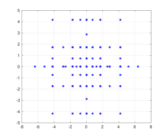
Figure 2. Index set $\mathcal{I}$ of the sparse-grid on the left and the associated sparse-grid points, which are used in the first numerical example, on the right.

Remark 2.1.

A further alternative could be to use multidimensional cubature formulas; see for instance, [9]. In principle, high-order cubature formulas also require smoothness of the integrand, therefore we suspect that the approach presented here will also work well in the cubature context. These methods are beyond the scope of the current paper.

3. Smoothing the payoff

In this section, we will describe a simple technique for smoothing the integrand in (4) which, at the same time,

• produces an analytic integrand;

• does not introduce a bias error;

• reduces the variance of the resulting integrand.

For the following, we assume that the covariance matrix $\Sigma$ is invertible (i.e., a positive definite symmetric matrix).

The general idea is that we want to integrate out one Gaussian factor in (4), conditioning on the remaining $d-1$ factors. Clearly, the outcome of such a procedure is a smooth function of the remaining factors. However, generically there is no closed formula for this function. The reason for this is that there is no closed formula for the simple special case

$$E\left[\left(e^{\sigma_{1}Z}+e^{\sigma_{2}Z}-K\right)^{+}\right]$$

for $Z\sim\mathcal{N}(0,1)$ and $\sigma_{1}\neq\sigma_{2}$. Indeed, $e^{\sigma_{1}Z}+e^{\sigma_{2}Z}$ has a log-normal distribution if and only if $\sigma_{1}=\sigma_{2}$. In this case, the above expression is given in terms of the celebrated Black-Scholes formula, which will be reviewed below.

It turns out, that a suitable choice of factorization of the covariance matrix of the Gaussian factors allows us to factor out one common, independent log-normal term. This is a consequence of the

Lemma 3.1.

Let $\Sigma$ be a symmetric, positive definite $d\times d$ matrix. Then there is for each vector $v\in\mathbb{R}^{d}$ a diagonal matrix $D=\operatorname{diag}\left(\lambda_{1}^{2},\lambda_{d}^{2},\ldots,\lambda_{d}^{2}\right)$ and an invertible matrix $V\in\mathbb{R}^{d\times d}$ with the property that $V_{i,1}\equiv v_{i}$, $i=1,\ldots,d$, and

$$\Sigma=VDV^{\top}.$$

Moreover, we may choose the remaining columns of $V$ such that $\lambda_{2}^{2}\geq\ldots\geq\lambda_{d}^{2}\geq 0$.

Proof.

From [3, p. 126], we know that for every ${0}\neq{s}\in\mathbb{R}^{n}$, the rank-1 modification

(13) $$\tilde{{A}}={A}-\frac{({As})({As})^{\top}}{{s}^{\top}{As}}$$

of a symmetric, positive definite matrix ${A}\in\mathbb{R}^{d\times d}$ yields a symmetric and positive semi-definite matrix $\tilde{A}\in\mathbb{R}^{d\times d}$ of rank $d-1$. Let us denote ${w}\coloneqq{\Sigma}^{-1}v$. Then it follows from (13) that

$$\tilde{\Sigma}={\Sigma}-\frac{vv^{\top}}{v^{\top}{w}}$$

is a symmetric and positive semi-definite matrix of rank $d-1$. Denote by $(\lambda_{i}^{2},{v}_{i})$ for $i=2,\ldots,d$ the $d-1$ eigenpairs corresponding to the $d-1$ positive eigenvalues of $\tilde{\Sigma}$. Defining $V=[{v}_{1},{v}_{2},\ldots,{v}_{d}]$ with ${v}_{1}=v$ and $D=\operatorname{diag}(\lambda_{1}^{2},\lambda_{2}^{2},\ldots,\lambda_{d}^{2})$ with $\lambda_{1}^{2}=(v^{\top}{w})^{-1}$ leads to the desired result. ∎

For the following computations, we choose the vector $v$ from Lemma 3.1 as $v=\mathbf{1}\coloneqq[1,\ldots,1]^{\top}$. In the next step, we replace $X$ by $Y\coloneqq V^{-1}X\sim\mathcal{N}(0,D)$ and note that the components of $Y$ are independent. By substituting the decomposition $X=VY$ into (4), we obtain

$$C_{\mathcal{B}} =E\left[\left(\sum_{i=1}^{d}w_{i}e^{(VY)_{i}}-K\right)^{+}\right]$$

$$=E\left[\left(\sum_{i=1}^{d}w_{i}\exp\left(Y_{1}+\sum_{j=2}^{d}V_{i,j}Y_{j}\right)-K\right)^{+}\right]$$

(14) $$=E\left[\left(h(Y_{2},\ldots,Y_{d})e^{Y_{1}}-K\right)^{+}\right]$$

with

(15) $$h(\overline{y})=h(y_{2},\ldots,y_{d})\coloneqq\sum_{i=1}^{d}w_{i}\exp\left(\sum_{j=2}^{d}V_{i,j}y_{j}\right),\quad\overline{y}\coloneqq(y_{2},\ldots,y_{d})\in\mathbb{R}^{d-1}.$$

Lemma 3.2 (Conditional Expectation formula).

Let $\overline{Y}=(Y_{2},\ldots,Y_{d})=((V^{-1}X)_{2},\ldots,(V^{-1}X)_{d})\sim\mathcal{N}\left(0,\overline{D}\right)$, $\overline{D}\coloneqq\operatorname{diag}(\lambda_{2}^{2},\ldots,\lambda_{d}^{2})$. Then

$$E\left[\left.\left(\sum_{i=1}^{d}w_{i}e^{X_{i}}-K\right)^{+}\right|\overline{Y}\right]=C_{BS}\left(h(\overline{Y})e^{\lambda_{1}^{2}/2},K,\lambda_{1}\right),$$

where

$$C_{BS}(S_{0},K,\sigma)\coloneqq\Phi(d_{1})S_{0}-\Phi(d_{2})K,$$

$$d_{1/2}\coloneqq\frac{1}{\sigma}\left[\log\left(\frac{S_{0}}{K}\right)\pm\frac{\sigma^{2}}{2}\right],$$

is the Black-Scholes formula for $r=0$, with maturity $T=1$.

Proof.

As $Y_{1}$ and $\overline{Y}$ are independent and $Y_{1}\sim\mathcal{N}(0,\lambda_{1}^{2})$, we have

$$E\left[\left.\left(h(Y_{2},\ldots,Y_{d})e^{Y_{1}}-K\right)^{+}\right|\overline{Y}=\overline{y}\right]=E\left[\left(h(\overline{y})e^{\lambda_{1}Z}-K\right)^{+}\right]$$

for some $Z\sim\mathcal{N}(0,1)$. On the other hand, for $r=0$ and maturity $T=1$, the Black-Scholes formula is given by

$$C_{BS}(S_{0},K,\sigma)=E\left[\left(S_{0}e^{-\frac{1}{2}\sigma^{2}+\sigma Z}-K\right)^{+}\right]=\Phi(d_{1})S_{0}-\Phi(d_{2})K,$$

since $S_{T}=S_{0}\exp\left(-\frac{1}{2}\sigma^{2}T+\sigma B_{T}\right)$ for a Brownian motion $B$. By comparing these expressions, we see that we have to choose $K=K$, $\sigma=\lambda_{1}$ and $S_{0}=h(\overline{y})e^{\frac{1}{2}\lambda_{1}^{2}}$. ∎

Lemma 3.2 directly implies

Proposition 3.3.

The basket option price in the multivariate Black-Scholes setting satisfies

(16) $$C_{\mathcal{B}}=E\left[C_{BS}\left(h\left(\sqrt{\overline{D}}Z\right)e^{\lambda_{1}^{2}/2},K,\lambda_{1}\right)\right],\quad Z\sim\mathcal{N}\left(0,I_{d-1}\right),\ \sqrt{\overline{D}}=\operatorname{diag}(\lambda_{2},\ldots,\lambda_{d}).$$

On the left-hand side of Figure 3, a visualization of the integrand in (4) before smoothing can be found while the corresponding smoothed integrand from (16) is presented on the right-hand side of Figure 3.

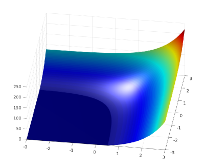
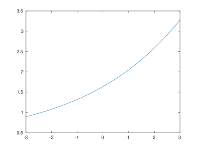
Figure 3. An example of a two-dimensional integrand with kink from (4) and its smoothed counterpart with respect to (16).

As remarked earlier, a similar closed-form expression cannot be obtained when the first column $V_{\cdot,1}$ of the matrix $V$ is a general $d$-dimensional vector. However, we may still get an explicit formula if $V_{\cdot,1}$ only takes values in $\set{0,1}$. For simplicity, let us assume that the first $k$ entries of $V_{\cdot,1}$ are $1$ and the remaining entries are $0$. The computation before Lemma 3.2 then gives

$$C_{\mathcal{B}}=E\left[\left(h_{1}(Y_{2},\ldots,Y_{k})e^{Y_{1}}+h_{2}(Y_{k+1},\ldots,Y_{d})-K\right)^{+}\right],$$

$$h_{1}(y_{2},\ldots,y_{k})\coloneqq\sum_{i=1}^{k}w_{i}\exp\left(\sum_{j=2}^{d}V_{i,j}y_{j}\right),$$

$$h_{2}(y_{k+1},\ldots,y_{d})\coloneqq\sum_{i=k+1}^{d}w_{i}\exp\left(\sum_{j=2}^{d}V_{i,j}y_{j}\right).$$

By conditioning again on $\overline{Y}$, we once again arrive at the Black-Scholes formula, this time requiring a shift in $K$ as well. In the end, we obtain

(17) $$E\left[\left.\left(\sum_{i=1}^{d}w_{i}e^{X_{i}}-K\right)^{+}\right|\overline{Y}\right]=C_{BS}\left(h_{1}(Y_{2},\ldots,Y_{k})e^{\lambda_{1}^{2}/2},K-h_{2}(Y_{k+1},\ldots,Y_{d}),\lambda_{1}\right),$$

in the sense that

$$C_{BS}(S_{0},K,\sigma)=S_{0}-K\text{ for }K<0.$$

In general, we therefore suggest to choose $V_{\cdot,1}$ such as to maximize the effective smoothing parameter $\lambda_{1}$.

More concretely, let us assume that the eigenvalues $\mu_{1}^{2}\geq\cdots\geq\mu_{d}^{2}>0$ of $\Sigma$ are given. Let $D=\operatorname{diag}\left(\mu_{1}^{2},\ldots,\mu_{d}^{2}\right)$. Of course, the matrix $Q\in O(d)$ of corresponding eigenvectors of $\Sigma$ satisfies

$$\Sigma=QDQ^{\top}.$$

Denoting $\lambda_{1}^{2}=\lambda_{1}^{2}(D,Q,v)=\left\langle v\,,\Sigma^{-1}v\right\rangle^{-1}$ and $\mathcal{V}\coloneqq\set{0,1}^{d}\setminus\set{0}$, we are looking for the worst possible smoothing effect given the eigenvalues $D$ of the covariance matrix $\Sigma$ and given that we choose the vector $v$ optimally, i.e., we are looking for

$$\lambda_{\ast}^{2}(D)\coloneqq\min_{Q\in O(d)}\max_{v\in\mathcal{V}}\lambda_{1}^{2}(D,Q,v).$$

Lemma 3.4.

We have $\lambda_{\ast}^{2}(D)\geq\mu_{d}^{2}$.

Proof.

We obviously have

$$\lambda_{\ast}^{2}(D)=\min_{Q\in O(d)}\max_{v\in\mathcal{V}}\lambda_{1}^{2}(D,Q,v)\geq\max_{v\in\mathcal{V}}\min_{Q\in O(d)}\lambda_{1}^{2}(D,Q,v)\geq\min_{Q\in O(d)}\lambda_{1}^{2}(D,Q,e_{d}),$$

for $e_{d}=(0,\ldots,0,1)$.

Clearly, the minimizing $Q$ should have $e_{d}$ as its last row, making $e_{d}$ the eigenvector corresponding to the smallest eigenvalue of $\Sigma$. Indeed, for any $Q\in O(d)$ we have

$$\lambda_{1}^{2}(D,Q,e_{d})=\left\langle Q^{\top}e_{d}\,,D^{-1}Q^{\top}e_{d}\right\rangle^{-1}=\left\langle q\,,D^{-1}q\right\rangle^{-1}=\left(\sum_{i=1}^{d}\frac{q_{i}^{2}}{\mu_{i}^{2}}\right)^{-1}\eqqcolon f(D,q),$$

where $q=q(Q)$ denotes the last row of $Q$ (understood as column vector). Note that the range of $q$ (as a function of $Q$) is $S_{d-1}$, hence we need to minimize $f(D,q)$ of all vectors $q$ with $q_{1}^{2}+\cdots+q_{d}^{2}=1$. It is easy to see that the minimizer is $q=e_{d}$ and the value is

$$\min_{Q\in O(d)}\lambda_{1}^{2}(D,Q,e_{d})=\mu_{d}^{2}.$$

In fact, we claim that the above lower bound holds uniformly over $v$ in the sense that

$$\max_{v\in\mathcal{V}}\min_{Q\in O(d)}\lambda_{1}^{2}(D,Q,v)=\mu_{d}^{2}.$$

The reason is that for arbitrary $v\in\mathcal{V}$ the minimizing $Q$ is still given such that $v$ is (up to normalization) the eigenvector corresponding to the smallest eigenvalue of $\Sigma$. Hence,

$$\min_{Q\in O(d)}\lambda_{1}^{2}(D,Q,v)=\left(\frac{\left\lvert v\right\rvert^{2}}{\mu_{d}^{2}}\right)^{-1}=\frac{\mu_{d}^{2}}{\left\lvert v\right\rvert^{2}}.$$

The equality follows by noting that $\min_{v\in\mathcal{V}}\left\lvert v\right\rvert^{2}=1$. ∎

Remark 3.5.

It is easy to check that the inequality in Lemma 3.4 is generally strict. We are not aware of more explicit expressions for $\lambda_{\ast}^{2}(D)$.

Remark 3.6.

It is worth observing that after the conditional expectation (16) one may also perform a change of measure on the resulting $d-1$ dimensions to enhance the convergence of all the quadratures discussed in this work. For instance, this is particularly important for OTM options.

4. Numerical example 1: Multivariate Black-Scholes setting

In our first numerical example, we consider the pricing problem (3) of a European basket option in a Black-Scholes model. This price depends on the strike price $K$, the weight vector $c$ and the vector $S_{T}$ containing the values of the different assets at the maturity $T$. Moreover, the distribution of $S_{T}$ can be deduced from the initial values of the assets $S_{0}$, the vector of volatilities $\sigma$ and the correlation matrix $\rho$, which determine the Black-Scholes model in (1). The initial values in our examples are chosen randomly, that is independently and uniformly distributed from the interval $S_{0}^{i}\in[8,20]$. The volatilities are also chosen randomly from the interval $\sigma_{i}\in[0.3,0.4]$. Following [11], the correlation matrix $\rho=\tau\tau^{\top}$ is given by a lower-triangular matrix $\tau$, parameterized by a vector $x\in[-1,1]^{d-1}$ as follows:

$$\tau_{1}=\begin{pmatrix}1\\ \operatorname{cp}(x)\end{pmatrix},\quad\tau_{2}=\sqrt{1-x_{1}^{2}}\begin{pmatrix}0\\ 1\\ \operatorname{cp}(x_{2:d-1})\end{pmatrix},\ldots,\quad\tau_{d}=\sqrt{1-x_{d-1}^{2}}\begin{pmatrix}0\\ \vdots\\ 0\\ 1\end{pmatrix}.$$

Herein, we employed the MATLAB-inspired notation $x_{2:d-1}=[x_{2},\ldots,x_{d-1}]^{\top}$. In addition, we denote by $\operatorname{cp}\colon\mathbb{R}^{d-1}\to\mathbb{R}^{d-1}$ the cumulative product given by

$$\operatorname{cp}(x)=[x_{1},x_{1}x_{2},\ldots,x_{1}x_{2}\cdots x_{d-1}]^{\top}.$$

Note that any such matrix is a proper correlation matrix, which only depends on $d-1$ (instead of $d(d-1)/2$) free parameters, and is therefore much easier to apply in practice. For sake of concreteness, we choose independently and uniformly distributed entries $x_{i}\in[0.8,1]$, which lead to positive correlations between the individual assets comprising the basket, a typical situation in equity markets. The weight vector $c$ is chosen such that the basket is an average of the different assets, i.e. $c_{i}=1/d$. Moreover, we choose three different settings for the strike price, $K=c^{\top}S_{0}$ (ATM), $K=1.2\cdot c^{\top}S_{0}$ (OTM) and $K=0.8\cdot c^{\top}S_{0}$ (ITM).

Remark 4.1.

We tested our experiments with different, randomly chosen weight vectors $c\in[0,1]^{d}$ and obtained similar results. Hence, it seems that there is only a slight dependence between the weight vector in the basket and the performance of the different quadrature methods.

We compare several integration schemes applied to the original problem (4) and the smoothened problem (16). To be more precise, we consider the MC method, the QMC method based on Sobol points and the sparse-grid method described in Section 2. Moreover, we also use a sparse grid approximation to the smoothed integrand as control variate to accelerate the convergence of MC and QMC. To keep track of the different quadratures that are used in the numerical examples, we summarize them together with their acronyms in table 1. Additionally, the colors and markers with which they appear in the convergence plots are listed here.

Method	Acronym	Color	Marker
Adaptive sparse grid to (4)	aSG		$\circ$
Quasi-Monte Carlo to (4)	QMC		$\circ$
Monte Carlo to (4)	MC		$\circ$
aSG to (16)	aSG+CS		$\star$
aSG with respect to (17)	aSG+CS2		$\star$
QMC to (16)	QMC+CS		$\star$
MC to (16)	MC+CS		$\star$
QMC to (16) with control variate	QMC+CS+CV		$\diamond$
MC to (16) with control variate	MC+CS+CV		$\diamond$

Table 1. Different quadrature methods, their acronyms, colors and markers.

4.1. Performance of the sparse-grid methods

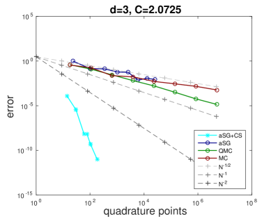
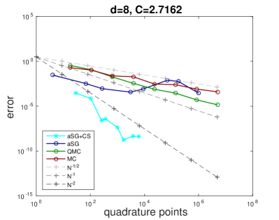
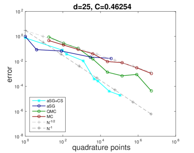
Figure 4. Errors for $d=3$, $d=8$ and $d=25$ with volatilities selected randomly from the interval $[0.3,0.4]$.

In this subsection, we investigate the convergence behaviour of the adaptive sparse-grid method for the smoothened problem (16) (aSG+CS). Therefore, we apply the (aSG+CS) to our model problem in dimension $d=3$ in the ATM case, $d=8$ in the ITM case and $d=25$ in the OTM case. Note that the ITM case is the easiest case and the OTM case is the hardest for numerical computation. The results would slightly improve when considering the ITM case in $d=25$ dimensions. However, we would like to demonstrate that the smoothing works well even for the hardest case in moderately high dimensions. As a reference solution, we use an adaptive sparse-grid quadrature to determine (16) with a very small tolerance, i.e. $\varepsilon=10^{-11}$ for $d=3$, $\varepsilon=10^{-9}$ for $d=8$, and $\varepsilon=10^{-7}$ for $d=25$ respectively. We use the listed Genz-Keister points from [24] as the sequence of underlying univariate quadrature points. Unfortunately, there exist only nine different Genz-Keister extensions and it might happen that a higher precision is needed in a particular direction. In this case, we use Gauß-Hermite quadratures with a successively higher degree of precision for the consecutive members of the quadrature sequence. The 1D Gauß-Hermite points and weights can easily be constructed for an arbitrary degree of precision by solving an associated eigenvalue problem; see [15] for the details.

To observe the convergence behaviour of the aSG+CS, we successively refine the tolerance (e.g., from $10^{-2}$ to $10^{-9}$ for $d=3$) and compute the relative error between the corresponding approximation to (16) and the reference solution. To compare the results with other methods and also to validate the reference solution, we also apply an MC quadrature, a QMC quadrature and an adaptive sparse-grid quadrature (SG) to the original problem (4) and compare the results with the reference solution as well. Herein, we increase the number of quadrature points for the (quasi-) Monte Carlo quadrature as $3\cdot 6^{q}$ for $q=1,\ldots,8$ which is adjusted for the sake of comparison with the aSG+CS method for the $25$-dimensional example. In addition, we use $20$ runs of the Monte-Carlo estimator on each level $q$ and plot the median of the relative errors to the reference solution of these $20$ runs.

The results for $d=3$, $d=5$ and $d=25$ are depicted in Figure 4. As expected, the MC quadrature converges in each dimension algebraically with a rate $1/2$ to the reference solution, while the rate of the QMC quadrature is close to $1$, despite the non-smooth integrand. The convergence of the aSG is comparable to that of the MC for $d=3$ and becomes worse for $d=8$ and $d=25$. Hence, it is not very suitable to tackle the original problem (4) with aSG. In contrast to that, the aSG+CS outperforms all other considered methods, especially for $d=3$ and $d=8$, in both convergence rate and constant. For $d=3$, the rate is exponential rather than algebraic and the observed algebraic rate for $d=8$ is $2$. In $d=25$ dimensions, the rate deteriorates to $1$ but the constant is still around a factor $35$ less than that of QMC.

Remark 4.2.

The convergence results are shown in terms of quadrature points. In case of adaptive sparse grids it might happen that the same quadrature point appears multiple times since we evaluate tensor products of difference quadrature formulas associated with multi-indices $\boldsymbol{\alpha}$. For example, for the approximation with tolerance $10^{-9}$ for d=$3$, the aSG+CS method requires $183$ quadrature points, but only $64$ of them are distinct, cf. Figure 2. Hence, the convergence results for adaptive sparse grid methods in terms of function evaluations at quadrature points could be improved if the function evaluations would be stored. However, it is also interesting to compare the computational times to see the overhead of the adaptive sparse-grid construction. In Table 2, we depict computational times in seconds and errors for the different quadrature methods at a comparable number of quadrature points for each dimension. As we can deduce from these times, there is indeed a huge overhead for the aSG+CS. In dimension $d=25$, for example, the computation of the adaptive sparse-grid method with around $25\%$ more quadrature points requires around $23$ times the computation time in comparison to QMC. Nevertheless, the error of the aSG+CS is around a factor $600$ smaller than that of QMC.

aSG+CS QMC MC time error points time error points time error points $d=3$ 0.0057 4.9 e-10 104 0.0016 1.25 e-1 108 0.0013 1.77 e-1 108 $d=8$ 0.3675 1.81 e-9 24622 0.0161 5.39 e-3 23328 0.0135 1.38 e-2 23328 $d=25$ 5.4283 1.04 e-6 174098 0.2409 6.18 e-4 139968 0.2188 1.29 e-3 139968

Table 2. Computation times for the different quadrature methods

Note that all the computations are done in MATLAB and that the evaluation of the integrand is completely vectorized in case of the (Q)MC. Naturally, this is not possible for the adaptive sparse-grid quadrature, since we adaptively add indices to the index set corresponding to difference quadrature rules with a relatively low number of quadrature points. Although the evaluation of the integrand in each difference quadrature rule is vectorized, we need to do this several times during the algorithm. Hence, a MATLAB implementation is not the most efficient one for adaptive sparse-grid quadratures or adaptive methods in general and the overhead could be reduced drastically with an efficient implementation in C, for example.

Finally, note that once an adaptive sparse grid has been constructed, it could potentially be re-used for pricing of options with similar parameters. In that case, of course, the overhead of constructing the sparse grid disappears completely.

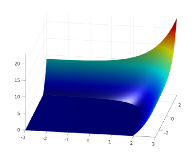
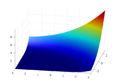
Figure 5. Projection on the first two variables of the Integrands in (4) (left) and (16) (right) for $d=25$ ( “out of the money”).

In summary, we find that the adaptive sparse-grid quadrature applied to (16) accurately approximates the value of a basket option. In particular, it significantly improves the performance of the adaptive sparse-grid quadrature applied to (4). This is due to the fact that the integrand in (16) is smooth while the integrand in (4) is not even differentiable. In order to corroborate the latter point, we illustrate in Figure 5 the projection on the first two variables of the $8$-dimensional integrand in (4) and of the $7$-dimensional integrand in (16) in the out of the money case. In addition to the smoothing effect, we further observe that the range of function values is reduced by around a factor $2.5$ for the latter integrand. Hence, it seems reasonable to additionally investigate the effects of the smoothing technique on the MC and QMC quadrature.

4.2. Smoothing effect for MC and QMC quadrature

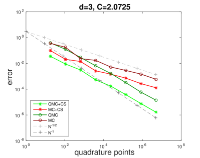
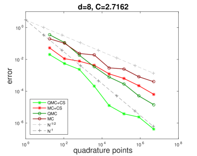
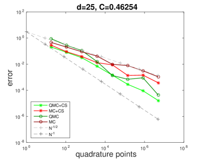
Figure 6. Smoothing effect for the (Q)MC quadrature for $d=3$, $d=8$ and $d=25$ with volatilities selected randomly from the interval $[0.3,0.4]$.

In this subsection, we examine the smoothing effect on the (Q)MC quadrature. To that end, we apply the (Q)MC quadrature with the same number of quadrature points as before (i.e. $3\cdot 6^{q}$ for $q=1,\ldots,8$) to approximate the integral in (16) and compare the results with those of the (quasi-) Monte Carlo quadrature applied to (4). For the Monte Carlo quadrature, we expect that the smoothing effect is not as strong as for the sparse-grid quadrature. Nevertheless, the convergence constant might be improved since we determined a conditional expectation to deduce (16) from (4), which should decrease the variance of the integrand. Figure 6 corroborates that the smoothing has the expected effect on the Monte Carlo quadrature, but the effect seems to diminish in higher dimensions. In case of the QMC quadrature, the smoothing does not effect the convergence rate but it does improve the convergence constant as well. Moreover, the effect is even stronger as for the Monte Carlo quadrature. The convergence constant of the QMC quadrature relies on the variation of the integrand and hence we suspect a larger decrease in the variation of the integrand than in the variance. This may be explained by the fact that the variation of a function can be calculated from the first mixed derivatives. Thus, the variation strongly depends on the smoothness of the integrand, in particular this dependence is stronger than for the variance of the integrand.

4.3. Acceleration by using a sparse-grid interpolant as a control variate

Another option to exploit the smoothness of the integrand is to combine a (Q)MC quadrature with a sparse-grid approximation. To that end, we construct a sparse-grid interpolant on the smoothened integrand in (16), that is we use sparse-grid quadrature nodes as interpolation points and employ this interpolant as a control variate. To explain the concept of a control variate, let us consider the integration problem of a function $f\colon\mathbb{R}^{d}\to\mathbb{R}$ and an approximation $g\colon\mathbb{R}^{d}\to\mathbb{R}$ on $f$. We assume that it is easy to calculate $E(g)\mathrel{\mathrel{\mathop{:}}=}\int_{\mathbb{R}^{d}}g(x)\operatorname{d\!}x$. Then, we rewrite the integral as

(18) $$\int_{\mathbb{R}^{d}}f(x)\operatorname{d\!}x=\int_{\mathbb{R}^{d}}f(x)-g(x)\operatorname{d\!}x+E(g).$$

Instead of using a (Q)MC estimate of the integral on the left-hand side of (18), we estimate the integral on the right-hand side. This means that the function $g\colon\mathbb{R}^{d}\to\mathbb{R}$ serves as a control variate, see for example [19] for a more detailed description. Of course, the quality of the control variate depends on how much the variance or the variation of $f-g$ is reduced compared with the variance or variation of $f$. Hence, it is closely connected to the approximation quality of $g$ on $f$.

In our examples, we use a total degree sparse-grid interpolant as a control variate. To describe that in more detail, let us denote by $\mathcal{I}_{j}\colon C(\mathbb{R})\to\mathcal{P}_{N_{j}}$ the interpolation operator at the $N_{j}$ quadrature points of the Gauß-Hermite quadrature with $N_{j}$ points. Then our sparse-grid interpolant $g$ is given by

$$g=\sum_{\alpha\in\mathbb{N}_{0}^{d}:\|\alpha\|_{1}\leq 2}\bigotimes_{j=1}^{d}(\mathcal{I}_{\alpha_{j}}-\mathcal{I}_{\alpha_{j}-1})f$$

with the convention $\mathcal{I}_{-1}\equiv 0$ and the numbers of quadrature points $N_{0}=1$, $N_{1}=3$ and $N_{2}=5$.

Remark 4.3.

The evaluation of this sparse-grid interpolant at the (Q)MC quadrature points becomes quite costly, especially in high dimensions. Most likely, more efficient control variates could be used, for example by including only the five most important dimensions in the sparse-grid interpolant. Nevertheless, the aim here is to demonstrate that it is possible, due to the smoothing, to significantly improve the convergence behaviour of the (Q)MC quadrature by a sparse-grid control variate on a relatively low level but we do not incorporate an efficiency analysis in terms of computational times here.

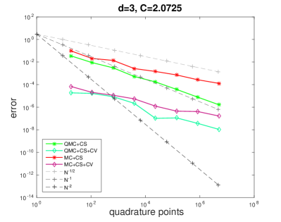
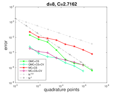
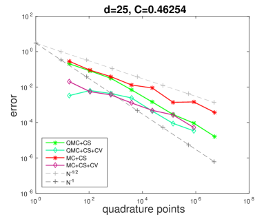
Figure 7. Acceleration of the (Q)MC quadrature with a sparse-grid control variate for $d=3$, $d=8$ and $d=25$ with volatilities selected randomly from the interval $[0.3,0.4]$.

The results of employing such a function as a control variate to improve the convergence of the (Q)MC+CS quadrature are visualized in Figure 7. The error reduction is quite impressive for both methods. In particular, the error of the MC+CS quadrature is reduced by a factor of approximately $10^{3}$ in $d=3$ dimension and still by a factor $10^{2}$ in $d=8$ and by a factor $30$ in $d=25$ dimensions while the convergence rate is preserved. In the case of the QMC+CS quadrature, the constant is reduced by a similar factor as in the Monte Carlo case. Although, the convergence rate seems to be slightly worse in comparison with the QMC+CS quadrature, the quasi-Monte Carlo quadrature with a sparse-grid control variate achieves the best error behaviour of the four considered methods in Figure 7 at least for $d=3$ and $d=8$.

5. Numerical example 2: Multivariate Variance-Gamma setting

In our second numerical example, we consider the pricing of a basket option in a multivariate Variance-Gamma model as introduced in [29]. Therefore, we recall that the multivariate extension of the univariate asset price process (6) is described as follows (cf. [28] and Section 1 above):

(19) $$S_{t}^{i}=S_{0}^{i}\exp\Big{(}(r+\omega_{i})t+\theta_{i}\gamma_{t}+\sigma_{i}W_{i}(\gamma_{t})\Big{)}$$

with

$$\omega_{i}=\frac{1}{\nu}\log\left(1-\frac{1}{2}\sigma_{i}^{2}\nu-\theta_{i}\nu\right).$$

We also incorporate here the deterministic interest rate $r$ in order to compare our results with those from [28]. The correlated $d$-dimensional Brownian motion $W$ in (19) is as in (2) given by its correlation matrix $\rho=\left(\rho_{i,j}\right)_{i,j=1}^{d}$ and its volatility vector $\sigma=[\sigma_{1},\ldots,\sigma_{d}]^{\top}$. The Gamma process $\gamma_{t}$ is independent from $W$ and described by the parameter $\nu$ via its density function

$$f_{\gamma_{t}}(y)=\frac{y^{1/\nu-1}}{\nu^{t/\nu}\Gamma(t/\nu)}e^{-y/\nu}.$$

The calculation of a European basket call option at time $T$ under the Variance-Gamma model leads then to

(20) $$C_{\mathcal{B}}\coloneqq\int_{0}^{\infty}e^{-rT}E\left[\left(\sum_{i=1}^{d}c_{i}S^{i}_{T}-K\right)^{+}\Bigg{|}\gamma_{T}=y\right]f_{\gamma_{T}}(y)\operatorname{d\!}y.$$

Herein, the integrand is for every fixed $y\geq 0$ just the value of a basket call option according to (3). Let us define

(21) $$w_{i} =c_{i}S^{i}_{0}e^{(r+\omega_{i})T},\quad i=1,\ldots,d,$$

$$\Sigma_{i,j} =\sigma_{i}\sigma_{j}\rho_{i,j}T,\quad i,j=1,\ldots,d.$$

Then, we can as in (4) rewrite the integrand in terms of a $d$-dimensional Gaussian vector $X^{y}=(X_{1}^{y},\ldots,X_{d}^{y})\sim\mathcal{N}(0,y\cdot\Sigma)$ to

$$E\left[\left(\sum_{i=1}^{d}c_{i}S^{i}_{T}-K\right)^{+}\Bigg{|}\gamma_{T}=y\right]=E\left[\left(\sum_{i=1}^{d}e^{\theta_{i}y}w_{i}e^{X_{i}}-K\right)^{+}\Bigg{|}\gamma_{T}=y\right].$$

Hence, we can apply the technique from Section 3 to equation (20). Therefore, we recall the decomposition of the matrix $\Sigma=VDV^{\top}$ according to Lemma 3.1. The first row of the matrix $V$ is the vector $v=[1,\ldots,1]^{\top}$ and we denote the entries of the diagonal matrix by $D=\operatorname{diag}(\lambda_{1}^{2},\ldots,\lambda_{d}^{2})$. Continuing in the same fashion as in Section 3, we end up with the equivalent integration problem (cf. (16)),

(22) $$C_{\mathcal{B}} =\int_{0}^{\infty}e^{-rT}E\left[C_{BS}\left(h_{y}\left(\sqrt{y\overline{D}}Z\right)e^{y\lambda_{1}^{2}/2},K,\sqrt{y}\lambda_{1}\right)\right]f_{\gamma_{T}}(y)\operatorname{d\!}y,$$

$$Z \sim\mathcal{N}\left(0,I_{d-1}\right),\ \sqrt{\overline{D}}=\operatorname{diag}(\lambda_{2},\ldots,\lambda_{d}).$$

Herein, the function $h_{y}$ is given similar as in (15) by

$$h_{y}(z_{2},\ldots,z_{d})\coloneqq\sum_{i=1}^{d}e^{\theta_{i}y}w_{i}\exp\left(\sum_{j=2}^{d}V_{i,j}z_{j}\right),\quad\overline{z}=(z_{2},\ldots,z_{d})\in\mathbb{R}^{d-1}.$$

Note that the integrand in (22) is very easy to calculate with respect to $y$ since we only need to incorporate the factor $e^{\theta_{i}y}$ in front of each weight $w_{i}$ and scale the matrix $D$ by $y$. Thus, the decomposition of the correlation matrix in view of Lemma 3.1 only has to be computed once although the correlation matrix of the Gaussian vector $X^{y}$ depends on the parameter $y$.

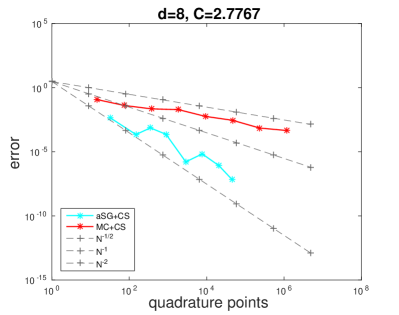
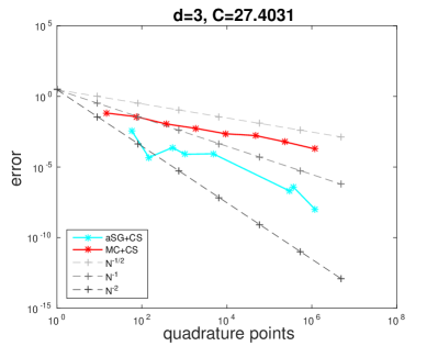
Figure 8. Errors of an ATM basket call under a Variance-Gamma model with parameters $\nu=0.3$ and $\theta_{i}\in[-0.1,0.05]$ for $d=8$ assets on the left and for an example from [28] with $d=3$ assets on the right.

In Figure 8, we present two examples for basket option pricing under the Variance-Gamma model. The first picture on the left-hand side depicts the error of the calculation of an ATM basket call (cf. (20)). We choose the parameters $r=0$ and $\nu=0.3$ in (19) deterministically and randomly select $\theta_{i}\in[-0.1,0.05]$. Moreover, the correlation matrix $\rho$, the volatilities $\sigma_{i}$ and the initial values $S_{0}^{i}$ in $d=8$ dimensions are constructed as in Section 4. We compare the convergence of the MC quadrature and the adaptive sparse-grid quadrature for the $d$-dimensional integral in (22). Note that the integration domain and the density function in (22) are given by

$$\Gamma=[0,\infty]\times\mathbb{R}^{d-1},\qquad p(y,z_{2},\ldots,z_{d})=f_{\gamma_{T}}(y)\cdot\frac{1}{(2\pi)^{d/2}}\exp\left(\frac{1}{2}\sum_{i=2}^{d}z_{i}^{2}\right).$$

Hence, we use $d$-dimensional random vectors where the first component is distributed with respect to $f_{\gamma_{T}}$ and independent to the remaining $d-1$ variables which are normally distributed and independent as well, as samples for the Monte-Carlo quadrature. In case of the adaptive sparse-grid quadrature, we apply tensor products of difference quadratures rules (cf. (11)), where we use differences of generalized Gauss-Laguerre quadrature rules as the quadrature sequence in the first variable. In the remaining variables, we set the univariate quadratures as in Section 4. Afterwards, we select the indices which are included in the sparse-grid adaptively as described in Section 2.2. As expected, the MC method converges exactly with a rate $N^{-1/2}$. Moreover, the result demonstrates that the adaptive quadrature outperforms the MC method even in this Variance-Gamma example with an observed rate of nearly $N^{-2}$.

The second numerical example is taken from the recent work [28] and stems originally from a parameter fitting of the Variance-Gamma model in [30]. It describes a 3D model as in (19) where $\theta=[-0.1368,-0.056,-0.1984]^{\top}$, $\sigma=[0.1099,0.1677,0.0365]^{\top}$ and $S_{0}=[100,200,300]^{\top}$. Additionally, the weight vector $c=[1/3,1/6,1/9]^{\top}$ and the correlation matrix

$$\rho=\begin{pmatrix}1&0.6&0.9\\ 0.6&1&0.8\\ 0.9&0.8&1\end{pmatrix}$$

were used. In [28], several different settings for the parameter $\nu$ and the strike price $K$ are considered. We restrict ourselves to the setting $\nu=0.5$ and $K=75$, which corresponds to an ITM basket. On the right-hand side of Figure 8 the convergence results for the MC and the adaptive approaches are shown. We observe that the MC quadrature converges as before. Although the convergence of the adaptive sparse-grid quadrature is still better than that of the Monte Carlo method, an exponential rate as could be expected for such a low-dimensional example cannot be obtained. This deterioration in the convergence rate does not depend on the Variance-Gamma setting but, as mentioned earlier, there is a connection of the smoothing to the entries of the diagonal matrix $D$ from Lemma 3.1. For the considered example, the matrix $D$ has the entries $\lambda_{1}^{2}=0.00023$, $\lambda_{2}^{2}=0.03432$ and $\lambda_{3}^{2}=0.00652$. In particular, the small value of $\lambda_{1}^{2}$ explains the relatively small smoothing effect. In view of (17), the vector $v=\mathbf{1}$ in Lemma 3.1 can be replaced by any other vector $0\neq v\in\{0,1\}^{d}$ to obtain a closed-form expression in Lemma 3.2.

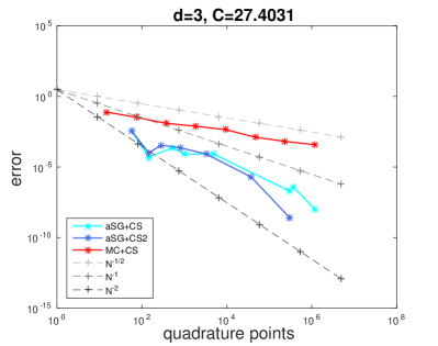
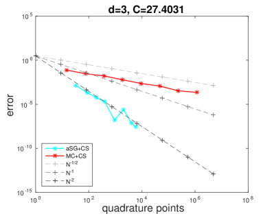
Figure 9. Errors for the example from [28] with $d=3$ assets. On the left-hand side, we included the convergence when the vector $\mathbf{1}$ is replaced by $v=[1,1,0]^{\top}$. On the right-hand side, we used the modified volatility $\sigma_{3}=0.1365$.

Therefore, we also investigated the convergence behaviour when we use a vector $v\neq\mathbf{1}$. We tested all possible choices of vectors $v\in\{0,1\}^{3}\setminus\{0\}$ and observed that $v=[1,1,0]^{\top}$ is best possible choice for this example. On the left-hand side of Figure 9, we compare the result from the right-hand side of Figure 8 with this best choice of $v$ denoted by (aSG+CS2) and observe an improved convergence, which comes together with a size of $\lambda_{1,v}^{2}=0.00109$, i.e. $\lambda_{1,v}^{2}$ is five times as high as $\lambda_{1}^{2}$. Nevertheless, $\lambda_{1,v}^{2}$ is still quite small compared with $\lambda_{2,v}^{2}=0.03294$ and, hence, the improvement in the convergence is not that extraordinary. This leads to the supposition that the considered example is not that well suited for our proposed method. In particular, the low value of $\sigma_{3}=0.0365$ compared with the other volatilities seems to have a negative effect on the smoothing. Hence, we tested this example also for the modified volatility $\sigma_{3}=0.1365$. The results for this case also depicted on the right-hand side of figure 9 show a drastically improved convergence. Furthermore, the entries of $D$ are given by $\lambda_{1}^{2}=0.01034$, $\lambda_{2}^{2}=0.02255$ and $\lambda_{3}^{2}=0.00526$, which demonstrates the influence of the differences in the volatilities on the size of $\lambda_{1}^{2}$ and thus on the smoothing.

Conclusions

In the context of basket options, we show that the inherent smoothing property of a Gaussian component of the underlying can be used to mollify the integrand (payoff function) without introducing an additional bias. Having obtained a smooth integrand, we can now directly apply (adaptive) sparse-grid methods. We observe that these methods are highly efficient in low and moderately high dimensions. For instance, the error can be improved by two orders of magnitude in dimension $25$ compared to (Q)MC methods. In dimension $3$, we even obtain exponential convergence. While the actual benefit of the smoothing method is very much problem dependent, we observed good results for the adaptive sparse grid method for the smoothed integrand up to dimension $35$ in the examples we considered. We have also discussed improvements for MC and QMC methods by introducing the smoothed payoff. In the Monte Carlo case, we do not observe a significant improvement in the computational error, as the variance reduction seems rather negligible. For QMC methods—Sobol numbers, to be more precise—we do see considerable improvements in the constant. As expected, the rate stays the same.

We note that the method employed in this work is not restricted to basket options in a multivariate Black-Scholes or Variance-Gamma setting, but can be generalized considerably. For instance, each step of an Euler discretization of an SDE corresponds to a Gaussian mixture model. Hence, the conditional expectation of the final integrand, given all the Brownian increments except for the last one, is in the form of a Gaussian integral of the payoff function w.r.t. to a normal distribution with possibly complicated mean vector and covariance matrix. If this integral can be computed explicitly, then we can directly obtain mollification of the payoff without introducing a bias.

Even if the integral cannot be computed in closed form, there may be use cases for employing numerical integration. For instance, in the basket option case, a fast and highly accurate numerical integration of the 1D log-normal integral, coupled with regression/interpolation (to avoid re-computation of the one-dimensional integral for each new (sparse) gridpoint) could turn out to be more efficient than a numerical integration technique applied to the full problem.

Finally, note that there are also clear limitations of the technique. For instance, consider a variation of the basket options studied in this work, namely a best-of-call option. Here, the payoff is given by

$$\left(\max_{i=1,\ldots d}S^{i}_{T}-K\right)^{+}$$

for log-normally distributed, correlated variables $S^{i}_{T}$ (in the Black-Scholes setting). Clearly, we can use Lemma 3.1 to construct a common normal factor $Y$ and other factors $Y_{1},\ldots,Y_{d}$ (all jointly normal, $Y$ independent of the rest), such that $S^{i}_{T}=e^{Y}e^{Y_{i}}$. Therefore, for the price of the best-of-call option, we obtain

$$E\left[\left(\max_{i=1,\ldots d}S^{i}_{T}-K\right)^{+}\right]=E\left[\left(e^{Y}\max_{i=1,\ldots d}e^{Y_{i}}-K\right)^{+}\right].$$

Taking the conditional expectation, we obtain the Black-Scholes formula applied at $\max_{i=1,\ldots d}e^{Y_{i}}$, which is still a non-smooth payoff. The mollification can only remove one source of irregularity in this case, not all of them. Indeed, as currently presented in this work, the conditional expectation step is most effective when the discontinuity surface of the option’s payoff has co-dimension one.

Acknowledgements

R. Tempone is a member of the KAUST Strategic Research Initiative, Center for Uncertainty Quantification in Computational Sciences and Engineering. C. Bayer and M. Siebenmorgen received support for research visits related to this work from R. Tempone’s KAUST baseline funds.

References

- [1] Nico Achtsis, Ronald Cools, and Dirk Nuyens. Conditional Sampling for Barrier Option Pricing Under the Heston Model, pages 253–269. Springer Berlin Heidelberg, Berlin, Heidelberg, 2013.
- [2] Nico Achtsis, Ronald Cools, and Dirk Nuyens. Conditional sampling for barrier option pricing under the LT method. SIAM J. Financial Math., 4(1):327–352, 2013.
- [3] W. Alt. Nichtlineare Optimierung: Eine Einführung in Theorie, Verfahren und Anwendungen. Vieweg+Teubner Verlag, 2002.
- [4] Christian Bayer, Peter K. Friz, and Peter Laurence. On the probability density function of baskets. In Large deviations and asymptotic methods in finance, volume 110 of Springer Proc. Math. Stat., pages 449–472. Springer, Cham, 2015.
- [5] Christian Bayer and Peter Laurence. Asymptotics beats Monte Carlo: the case of correlated local vol baskets. Comm. Pure Appl. Math., 67(10):1618–1657, 2014.
- [6] Christian Bayer and Peter Laurence. Small-time asymptotics for the at-the-money implied volatility in a multi-dimensional local volatility model. In Large deviations and asymptotic methods in finance, volume 110 of Springer Proc. Math. Stat., pages 213–237. Springer, Cham, 2015.
- [7] H.-J. Bungartz and M. Griebel. Sparse grids. Acta Numerica, 13:147–269, 2004.
- [8] R. Caflisch. Monte Carlo and quasi-Monte Carlo methods. Acta Numerica, 7:1–49, 1998.
- [9] Ronald Cools. An encyclopaedia of cubature formulas. Journal of Complexity, 19(3):445 – 453, 2003. Oberwolfach Special Issue.
- [10] Josef Dick, Frances Y Kuo, and Ian H Sloan. High-dimensional integration: the quasi-monte carlo way. Acta Numerica, 22:133–288, 2013.
- [11] Paul Doust. Two useful techniques for financial modelling problems. Applied Mathematical Finance, 17(3):201–210, 2010.
- [12] Daniel Dufresne. The log-normal approximation in financial and other computations. Adv. in Appl. Probab., 36(3):747–773, 2004.
- [13] Eric Fournié, Jean-Michel Lasry, Jérôme Lebuchoux, Pierre-Louis Lions, and Nizar Touzi. Applications of Malliavin calculus to Monte Carlo methods in finance. Finance Stoch., 3(4):391–412, 1999.
- [14] Jim Gatheral. The Volatility Surface: A Practitioner’s Guide. Wiley, 2006.
- [15] John H. Welsch Gene H. Golub. Calculation of gauss quadrature rules. Mathematics of Computation, 23(106):221–s10, 1969.
- [16] Alan Genz and B.D. Keister. Fully symmetric interpolatory rules for multiple integrals over infinite regions with gaussian weight. Journal of Computational and Applied Mathematics, 71(2):299 – 309, 1996.
- [17] T. Gerstner and M. Griebel. Dimension–adaptive tensor–product quadrature. Computing, 71(1):65–87, 2003.
- [18] Thomas Gerstner. Sparse grid quadrature methods for computational finance. Habilitation, University of Bonn, 77, 2007.
- [19] P. Glasserman. Monte Carlo Methods in Financial Engineering. Applications of mathematics : stochastic modelling and applied probability. Springer, 2004.
- [20] M. Griebel, F. Y. Kuo, and I. H. Sloan. The smoothing effect of integration in and the ANOVA decomposition. Math. Comp., 82:383–400, 2013. Also available as INS preprint No. 1007, 2010.
- [21] M. Griebel, F. Y. Kuo, and I. H. Sloan. The ANOVA decomposition of a non-smooth function of infinitely many variables can have every term smooth. Submitted to Mathematics of Compuation. Also available as INS preprint No. 1403, 2014, 2014.
- [22] M. Griebel, F. Y. Kuo, and I. H. Sloan. Note on ”The smoothing effect of integration in and the ANOVA decomposition”. Submitted to Mathematics of Compuation. Also available as INS preprint No. 1513, 2015.
- [23] J. M. Hammersley and D. C. Handscomb. Monte Carlo methods. Methuen, London, 1964.
- [24] Florian Heiss and Viktor Winschel. Likelihood approximation by numerical integration on sparse grids. Journal of Econometrics, 144(1):62–80, 2008.
- [25] Markus Holtz. Sparse Grid Quadrature in High Dimensions with Applications in Finance and Insurance. Springer Verlag, Berlin, Heidelberg, 2011.
- [26] Martin Krekel, Johan de Kock, Ralf Korn, and Tin-Kwai Man. An analysis of some methods for pricing basket options. Wilmott, pages 82–89, 2004.
- [27] Pierre L’Ecuyer. Quasi-Monte Carlo methods with applications in finance. Finance and Stochastics, 13(3):307–349, 2009.
- [28] Daniël Linders and Ben Stassen. The multivariate variance gamma model: basket option pricing and calibration. Quantitative Finance, 0(0):1–18, 0.
- [29] Elisa Luciano and Wim Schoutens. A multivariate jump-driven financial asset model. Quantitative Finance, 6(5):385–402, 2006.
- [30] Dilip B. Madan, Peter P. Carr, and Eric C. Chang. The variance gamma process and option pricing. Eur. Finance Rev., 2(1):79–105, 1998.
- [31] H. Niederreiter. Random Number Generation and Quasi-Monte Carlo Methods. Society for Industrial and Applied Mathematics, Philadelphia, PA, 1992.
- [32] Marc Romano and Nizar Touzi. Contingent claims and market completeness in a stochastic volatility model. Math. Finance, 7(4):399–412, 1997.
- [33] S. Smolyak. Quadrature and interpolation formulas for tensor products of certain classes of functions. Doklady Akademii Nauk SSSR, 4:240–243, 1963.
- [34] I.M Sobol’. On the distribution of points in a cube and the approximate evaluation of integrals. USSR Computational Mathematics and Mathematical Physics, 7(4):86 – 112, 1967.