$\mathcal{P}\mathcal{T}$-symmetric slowing-down of decoherence

Abstract

We investigate $\mathcal{P}\mathcal{T}$-symmetric quantum systems ultra-weakly coupled to an environment. We find that such open systems evolve under $\mathcal{P}\mathcal{T}$-symmetric, purely dephasing and unital dynamics. The dynamical map describing the evolution is then determined explicitly using a quantum canonical transformation. Furthermore, we provide an explanation of why $\mathcal{P}\mathcal{T}$-symmetric dephasing type interactions lead to critical slowing down of decoherence. This effect is further exemplified with an experimentally relevant system – a $\mathcal{P}\mathcal{T}$-symmetric qubit easily realizable, e.g., in optical or microcavity experiments.

Introduction.

Symmetry is one of the most important and profound concepts in physics Weyl (1952); Gross (1996) which explains the modus operandi of many complex physical and biological systems Breier et al. (2016). It expresses how systems remain unaffected by perturbations Peres (1995). Therefore, a violation of symmetry (or its breakdown J. Zhang et al. (2015)) constitutes an irreplaceable source of valuable information regarding properties of physical systems Higgs (1964); Ge and Stone (2014); Zhu et al. (2016). There is an abundance of useful transformations providing necessary ingredients to understand and investigate quantum systems. Among them, there are two of special physical significance: the time reversal operation $\mathcal{T}$ Crooks (2008) and parity – a mirror-reflection symmetry – $\mathcal{P}$ Zeng et al. (2005). These two transformations are both hermitian and independent of each other, i.e., $[\mathcal{P},\mathcal{T}]=0$. Systems that are invariant under the joint $\mathcal{P}\mathcal{T}$ operation are called $\mathcal{P}\mathcal{T}$-symmetric Bender et al. (2002). Such effectively open systems exhibit dynamics with balanced loss and gain Jing et al. (2014); Sounas et al. (2015). Recent results have proven to be of great theoretical Gardas et al. (2016a); Kartashov et al. (2015); Hang et al. (2013); Bender and Boettcher (1998) and experimental Lawrence et al. (2014); Rüter et al. (2010); Longhi (2010); T. Gao et al. (2015) importance, and $\mathcal{P}\mathcal{T}$-symmetric quantum systems have been realized in many different setups, such as optical A. Guo et al. (2009), optomechanical Lü et al. (2015) or microcavity based experiments B. Peng et al. (2014); Jing et al. (2014).

Contemporary studies have revealed that important (non)equilibrium properties and thermodynamic relations also hold for $\mathcal{P}\mathcal{T}$-symmetric quantum systems; e.g., the Carnot theorem Gardas et al. (2016a); Jiang et al. (2015) and the Jarzynski equality Jarzynski (1997); Deffner and Saxena (2015). Nevertheless, to further advance our understanding of $\mathcal{P}\mathcal{T}$-symmetric quantum systems the next natural step is to understand decoherence Zurek (2003). This is particularly important when one wants to store and process information in quantum systems Mohseni et al. (2003); Ladd et al. (2010); Pellizzari et al. (1995).

A comprehensive description of the system’s dynamics requires tracing out the environmental degrees of freedom. Unfortunately, except for a few analytically solvable models, finding such reduced dynamics $\varrho_{\text{S}}(t)$ has proven to be extremely complicated, often impossible, even for hermitian systems Breuer and Petruccione (2002). Recently, it has been shown that all $\mathcal{P}\mathcal{T}$-symmetric quantum systems that admit real spectrum can be represented in a physically equivalent way by hermitian Hamiltonians Gardas et al. (2016b). One would therefore expect them to be influenced by decoherence in a similar manner. In this Letter, however, we demonstrate features that are unique to $\mathcal{P}\mathcal{T}$-symmetric systems, resulting from the way they interact with their environment. In particular, we investigate a $\mathcal{P}\mathcal{T}$-symmetric quantum system coupled ultra-weakly to a hermitian environment Spohn and Lebowitz (2007). Our motivation is twofold: First, very weak coupling guarantees that no heat is exchanged between the system and environment Averin et al. (2016); A. Thoma et al. (2016). This leads to a phenomenon known as pure decoherence or dephasing Cummings and Roche (2016); Chesi et al. (2016). Only quantum information is allowed to enter or leave the system so that any effect caused solely by decoherence can be quantified easily. Finally, following the Ockham’s razor principle Sober (2015), hermiticity of the environment is assumed for the sake of simplicity and transparency of our description.

Under these assumptions, we find that such open systems evolve under $\mathcal{P}\mathcal{T}$-symmetric, purely dephasing and unital dynamics. The dynamical map describing the evolution is then determined explicitly using a quantum canonical transformation. Therefore, as an immediate consequence of dephasing and unital dynamics we find the validity of the Jarzynski equality Rastegin and Życzkowski (2014). Furthermore, we explain how a $\mathcal{P}\mathcal{T}$-symmetric dephasing channel leads to critical slowing down of decoherence. This effect is exemplified using an experimentally relevant example – a $\mathcal{P}\mathcal{T}$-symmetric qubit. Such a two-level system can be realized e.g. in optics Rüter et al. (2010) or in a microcavity T. Gao et al. (2015). In particular, in the development of practical architectures for quantum computer systems with minimal or suppressed decoherence are appealing Lidar et al. (1998); M. W. Johnson et al. (2011). We will see that $\mathcal{P}\mathcal{T}$-symmetric qubits are thus significantly better suited than standard, hermitian qubits T. Lanting et al. (2014).

Pure decoherence in $\mathcal{P}\mathcal{T}$-symmetric quantum systems.

Consider a $\mathcal{P}\mathcal{T}$-symmetric quantum system $S$ interacting with its environment, $B$. The composite system $S+B$ can be described by the following Hamiltonian

$$H=H_{\text{S}}\otimes\mathbb{I}_{\text{B}}+\mathbb{I}_{\text{S}}\otimes H_{\text{B}}+H_{\text{I}},$$ (1)

where $H_{\text{S}}$ and $H_{\text{B}}$ are the Hamiltonians of the system and the environment respectively, and $H_{\text{I}}$ describes the interaction between them. In the following, we assume the usual form of the interaction: $H_{\text{I}}=V_{\text{S}}\otimes V_{\text{B}}$, where both $H_{\text{B}}$ and $V_{\text{B}}$ are hermitian yet $V_{\text{S}}$ is $\mathcal{P}\mathcal{T}$-symmetric. Typical examples include $\mathcal{P}\mathcal{T}$-symmetric resonators coupled weakly to the rest of the (hermitian) Universe Phang et al. (2015). A particularly interesting example arises when $V_{\text{S}}=g(H_{\text{S}})$, where $g$ is an arbitrary function. Since $[H_{\text{S}},H_{\text{I}}]=0$, there is no energy exchange between the system and its environment; i.e., $\langle H_{\text{S}}\rangle$ remains constant during the evolution. Therefore, any effect of the environment on the system leads to pure decoherence Alicki (2004). Without any loss of generality we further assume that $g(H_{\text{S}})=H_{\text{S}}$.

Henceforth, we focus on $\mathcal{P}\mathcal{T}$-symmetric quantum systems and show how to construct their reduced dynamics in the presence of pure decoherence. To this end, we notice that if the spectrum of the system is real a hermitian transformation $T$ such that $h_{\text{S}}=TH_{\text{S}}T^{-1}$ is hermitian can always be found Gardas et al. (2016a). Moreover, since $h_{\text{S}}$ is hermitian we also have $H_{\text{S}}^{\dagger}=T^{2}H_{\text{S}}T^{-2}$ which will be crucial for our analysis. We will prove this shortly. Here, we only note that in order to change hermiticity such a transformation cannot be unitary. However, $T$ preserves (canonical) commutation relations (e.g. between $x$ and $p$: $[x,p]=i\hbar$) and therefore will be regarded as a quantum canonical transformation Anderson (1994); Lee and l’Yi (1995). More importantly, canonical transformations do not change expectation values of observables: $\langle O_{\text{S}}\rangle_{\mathcal{P}\mathcal{T}}=\langle o_{\text{S}}\rangle_{H}$ where $o_{\text{S}}=TO_{\text{S}}T^{-1}$.

Now, applying the canonical transformation $T$ to the Hamiltonian (1) yields

$$h=h_{\text{S}}\otimes\mathbb{I}_{\text{B}}+\mathbb{I}_{\text{S}}\otimes H_{\text{B}}+h_{\text{I}},\quad h_{\text{I}}=TH_{\text{I}}T^{-1},$$ (2)

where $T$ acts nontrivially only on the system of interest. Since the two systems are now hermitian their composed dynamics is described by the Liouville-von Neumann equation of motion, $i\dot{\varrho}(t)=[h,\varrho(t)]$, whose unique solution can be written as Breuer and Petruccione (2002)

$$\varrho(t)\rightarrow U(t)\varrho(0)U(t)^{\dagger},\quad U(t)=\exp(-iht).$$ (3)

At any given time $t$, the reduced system’s dynamics is determined by tracing out the environmental degrees of freedom (see e.g. Alicki and Lendi (2007)). Thus, one can write

$$\varrho_{\text{S}}(t)=\text{tr}_{\text{B}}\{U(t)\varrho_{\text{S}}(0)\otimes\Omega_{\text{B}}U(t)^{\dagger}\},$$ (4)

where $\Omega_{\text{B}}$ is the initial state of the environment and $\text{tr}_{\text{B}}\{\cdot\}$ denotes the partial trace Alicki and Lendi (2007). Note that the two systems are uncorrelated at $t=0$ Ringbauer et al. (2015). This requirement is crucial for the map $\Phi$: $\varrho_{\text{S}}(t)=\Phi[\varrho_{\text{S}}(0)]$ to be well defined Štelmachovič and Bužek (2001); *Buzek01a. However, this is not difficult to fulfill experimentally Chen and Goan (2016).

Since $\Omega_{\text{B}}$ is a density operator, it can be expressed as $\Omega_{\text{B}}=\sum_{\alpha}p_{\alpha}\left|\alpha\right\rangle\left\langle\alpha\right|$, where $p_{\alpha}$ denotes the probability of finding the environment in state $\left|\alpha\right\rangle$. As a result, the reduced dynamics (4) can be rewritten using the so called operator-sum representation Schlosshauer (2005):

$$\varrho_{\text{S}}(t)=\textstyle{\sum_{i}}K_{i}(t)\varrho_{\text{S}}(0)K_{i}(t)^{\dagger},$$ (5)

where the Kraus operators $K_{i}(t)=\sqrt{p_{\alpha}}\left\langle\beta\right|U(t)\left|\alpha\right\rangle$ satisfy $\sum_{i}K_{i}(t)^{\dagger}K_{i}(t)=\mathbb{I}_{\text{S}}$. To simplify notation we have combined the two indices $\alpha$, $\beta$ into $i$. Moreover, Eq. (5) defines a unital map, i.e. $\Phi[\mathbb{I}_{\text{S}}]=\mathbb{I}_{\text{S}}$ Rastegin and Życzkowski (2014). Indeed, since $h_{\text{S}}$ commutes with $h$ we also have $[K_{i}(t),K_{i}(t)^{\dagger}]=0$ .

The operator-sum representation in Eq. (5) provides the most general description of decoherence and dissipation for hermitian quantum systems, which results from the interaction with the environment. It is often referred to as a quantum channel, i.e., a map that is completely positive and trace preserving - CPTP Nielsen and Chuang (2011). When there is only one Kraus operator the evolution is unitary . Multiplying Eq. (5) from both sides by $T^{-1}$ and $T$, respectively, yields

$$\rho_{\text{S}}(t)=T^{-1}\varrho_{\text{S}}(t)T=\textstyle{\sum_{i}}L_{i}(t)\rho_{\text{S}}(0)R_{i}(t),$$ (6)

where the left, $L_{i}(t)$, and right, $R_{i}(t)$, Kraus operators read

$$L_{i}(t)=T^{-1}K_{i}(t)T,\quad R_{i}(t)=T^{-1}K_{i}(t)^{\dagger}T.$$ (7)

We see immediately that they fulfill $\sum_{i}L_{i}(t)R_{i}(t)=\mathbb{I}_{\text{S}}$. The last equality assures that the $\mathcal{P}\mathcal{T}$-CPTP map (7) is unital as well Rastegin (2013); Kafri and Deffner (2012); Albash et al. (2013). Therefore, $\mathcal{P}\mathcal{T}$-symmetric, purely dephasing and unital dynamics preserve the Jarzynski equality . Similar conclusions have been drawn recently for $\mathcal{P}\mathcal{T}$-symmetric Schrödinger dynamics Deffner and Saxena (2015). Note, when the dynamics is unitary then $L(t)=U(t)$ and $R(t)=U(-t)$, where $U(t)$ satisfies the Schrödinger equation. We emphasize, however, that $U(t)^{\dagger}\not=U(-t)$.

In summary, Eq. (6) provides the most general description of open $\mathcal{P}\mathcal{T}$-symmetric quantum systems. This is our main result. To this end, we followed the following recipe: First, one transforms the $\mathcal{P}\mathcal{T}$-symmetric Hamiltonian into its hermitian representation using a quantum canonical transformation. Next, after solving the corresponding equation of motion, the inverse map is applied to obtain the final solution . Our approach is generic and can be applied to e.g. Lindblad master equations Dast et al. (2014); T. Prosen (2012) or quantum Brownian motion Lampo et al. (2016); Hänggi and Marchesoni (2009). Also, our strategy is not restricted just to Markovian dynamics Zhang et al. (2012). However, for the present purposes we have chosen a model without heat exchange between system and environment Alicki (2004).

Canonical transformation.

As we have seen, to obtain the reduced dynamics for an open $\mathcal{P}\mathcal{T}$-symmetric system one needs to construct a canonical transformation $T$ that restores hermiticity Gardas et al. (2016a). To this end, we assume that all energies of $H_{\text{S}}$ are real and experimentally accessible. For the sake of simplicity, we also assume that the spectrum of $H_{\text{S}}$ is discrete and non-degenerate. Therefore, there exists a basis $\left|E_{n}\right\rangle$ in which all energies $E_{n}$ can be measured. Hence, $VH_{\text{S}}V^{-1}=\sum_{n}E_{n}\left|E_{n}\right\rangle\left\langle E_{n}\right|$, where $\left\langle E_{n}|E_{m}\right\rangle=\delta_{nm}$ and all energies $E_{n}$ are real. Now, the canonical transformation $T$ can be calculated as $T=\sqrt{V^{\dagger}V}$. Note, since $H_{\text{S}}$ is not hermitian $V$ is not unitary (i.e., $V^{\dagger}\not=V^{-1}$). To show this elegant and simple result we first notice that $H_{\text{S}}$ can also be rewritten as 

$$H_{\text{S}}=\textstyle{\sum_{n}}E_{n}\left|\psi_{n}\right\rangle\left\langle\phi_{n}\right|.$$ (8)

The new eigenstates $\left|\psi_{n}\right\rangle=V^{-1}\left|E_{n}\right\rangle$ and $\left\langle\phi_{n}\right|=\left\langle E_{n}\right|V$ form a biorthonormal basis Vujicic (2008); Mostafazadeh (2002). That is to say, the following orthogonality and completeness relations hold: $\left\langle\psi_{n}|\phi_{n}\right\rangle=\delta_{nm}$ and $\sum_{n}\left|\psi_{n}\right\rangle\left\langle\phi_{n}\right|=\mathbb{I}_{\text{S}}$. Biorthonormality also means that $\left|\psi_{n}\right\rangle$, $\left|\phi_{n}\right\rangle$ are the left and right eigenstates of $H_{\text{S}}$, respectively. The corresponding eigenenergy reads $E_{n}$. Since $H_{\text{S}}$ is $\mathcal{P}\mathcal{T}$-symmetric, it follows that Weigert (2003)

$$\mathcal{P}H_{\text{S}}\mathcal{P}=\mathcal{T}H_{\text{S}}\mathcal{T}=H_{\text{S}}^{\dagger}.$$ (9)

From the last equation we have $\mathcal{P}\left|\psi_{n}\right\rangle=e^{i\theta_{n}}\left|\phi_{n}\right\rangle$, where $\theta_{n}=0$, $\pi$. Now, $T$ can be decomposed as $T^{2}=\mathcal{P}\mathcal{C}$, where the charge conjugation $\mathcal{C}$ reads Weigert (2003)

$$\mathcal{C}=\textstyle{\sum_{n}}\left|\psi_{n}\right\rangle\left\langle\psi_{n}\right|\mathcal{P}\quad\text{(note}\quad\mathcal{C}^{2}=\mathbb{I}_{\text{S}}\text{)}.$$ (10)

By construction, the charge conjugation commutes with the system Hamiltonian $H_{\text{S}}$ and thus from Eq. (9) it follows immediately that $T^{2}\,H_{\text{S}}\,T^{-2}=H_{\text{S}}^{\dagger}$ . Finally,

$$h_{\text{S}}^{\dagger}=T^{-1}\left(T^{2}\,H_{\text{S}}\,T^{-2}\right)T=h_{\text{S}}.$$ (11)

In conclusion, the canonical map $T$ indeed transforms a $\mathcal{P}\mathcal{T}$-symmetric Hamiltonian $H_{\text{S}}$ into a hermitian one, $h_{\text{S}}$. The main results (6)-(7) hold for all $\mathcal{P}\mathcal{T}$-symmetric quantum systems that admit real spectra .

Critical slowing down of decoherence.

The remainder of our work is dedicated to studying an experimentally relevant example T. Gao et al. (2015). Consider a $\mathcal{P}\mathcal{T}$-symmetric qubit :

$$H_{\text{S}}=\alpha\sigma_{+}\sigma_{-}+\gamma\sigma_{+}+\text{h.c.}=\begin{pmatrix}\alpha&\gamma\\ \gamma^{*}&\alpha^{*}\end{pmatrix},$$ (12)

where both $\alpha$ and $\gamma$ can be complex parameters, whereas $\sigma_{+}$ and $\sigma_{-}$ are the raising and lowering fermionic operators. This simple model has been extensively studied in the literature Deffner and Saxena (2015); Bender et al. (2002, 2003). Moreover, it has also been realized experimentally both in optics Rüter et al. (2010) and semiconductor microcavities T. Gao et al. (2015). We assume the system (12) to be coupled to a bosonic heat bath at the inverse temperature $\beta$ via a dephasing interaction. That is to say

$$H_{\text{B}}=\textstyle{\sum_{n}}\omega_{n}a_{n}^{\dagger}a_{n},\quad V_{\text{B}}=\textstyle{\sum_{n}}g_{n}\left(a_{n}+a_{n}^{\dagger}\right),$$ (13)

where $a_{n}$, $a_{n}^{\dagger}$ are the bosonic creation and annihilation operator, respectively Kumar et al. (2013). They obey the canonical commutation relation $[a_{n},a_{m}^{\dagger}]=\delta_{nm}$. The bath’s eigenmodes $\omega_{n}$ and coupling constants $g_{n}$ are assumed to be real. We emphasize that the above bosonic Hamiltonians are hermitian Sober (2015). Nevertheless, they do not commute, i.e. $[H_{\text{B}},V_{\text{B}}]\not=0$. This results in nontrivial dynamics and decoherence.

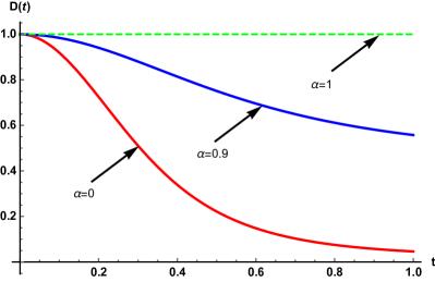
Figure 1: (Color online): Critical slowing down of decoherence. The decoherence function $D(t)$ decays more gradually as $\alpha$ increases. Eventually, it becomes constant at the critical point $\alpha=1$. Red line corresponds to a hermitian system ($\alpha=0$). Parameters are: $\mu=-0.5$, $\,\beta=0.5$ and $J_{0}=\omega_{c}=1$. For negative $\alpha$ the situation is symmetric [see e.g. Eq. (18)].

In the following, we explicitly construct the hermitian representation of Hamiltonian (12). Without any loss of generality, we can choose $\alpha$ to be purely imaginary, i.e. $\alpha\rightarrow i\alpha$; we will also set $\gamma=1$. Then, as long as $|\alpha|\leq 1$, the spectrum of $H_{\text{S}}$ is real. It consists of two eigenvalues: $E_{1,2}=\mp\sqrt{1-\alpha^{2}}$. Simple calculations show that Gardas et al. (2016a)

$$T=U^{\dagger}\begin{pmatrix}s_{1}&0\\ 0&s_{2}\end{pmatrix}U,\quad U=\frac{1}{\sqrt{2}}\begin{pmatrix}i&1\\ -i&1\end{pmatrix},$$ (14)

where $s_{1,2}=\sqrt{2(1\pm\alpha)}$ and $U$ is unitary. Therefore, the corresponding hermitian Hamiltonian reads

$$h_{\text{S}}=E_{1}\sigma_{x}=\begin{pmatrix}0&E_{1}\\ E_{1}&0\end{pmatrix},$$ (15)

where $\sigma_{x}$ is the Pauli-$x$ matrix. The resulting model describes the paradigmatic spin-boson system with effective couplings $g_{n}E_{1}$ Fannes et al. (1988).

In what follows, we assume the initial state of the environment to be the Gibbs state, $\Omega_{\text{B}}=\exp(-\beta H_{\text{B}})/Z$, where $Z=\text{tr}\{\exp(-\beta H_{\text{B}})\}$ is the partition function Callen (1985). The reduced dynamics $\varrho(t)=[\varrho_{ij}(t)]_{2\times 2}$ can be obtained exactly Gardas (2011). Indeed, we have Łuczka (1990)

$$\begin{split}\varrho_{11}(t)&=\frac{1}{2}-\Re[\varrho_{12}(0)e^{-iE_{1}t}]\,D(t),\\ \varrho_{12}(t)&=\varrho_{11}(0)-\frac{1}{2}+i\Im[\varrho_{12}(0)e^{-iE_{1}t}]\,D(t),\end{split}$$ (16)

Moreover, $\varrho_{22}(t)=1-\varrho_{11}(t)$ and $\varrho_{21}(t)=\varrho_{12}(t)^{*}$ . Above, symbols $\Re(z)$ and $\Im(z)$ denote the imaginary and real parts of a complex number $z$, respectively, whereas the decoherence function $D(t)=\exp(-E_{1}^{2}\gamma(t))$ quantifies decoherence Baumgratz et al. (2014). Information regarding the environment is encoded in the temperature-dependent function $\gamma(t)$,

$$\gamma(t)=\int_{0}^{\infty}\,d\omega\frac{J(\omega)}{\omega^{2}}\,\left(1-\cos\omega t\right)\coth\left(\frac{\hbar\beta\omega}{2}\right),$$ (17)

where $J(\omega)=\sum_{n}|g_{n}|^{2}\delta(\omega-\omega_{n})$ is the spectral density that characterizes the environment. Typical examples include $J(\omega)=J_{0}\omega^{1+\mu}\exp(-\omega/\omega_{c})$ for some predefined constants $J_{0}$, $\mu$ and $\omega_{c}$ Leggett et al. (1987). For example, when $\mu=0$ (Ohmic case) and $\beta\omega_{c}\gg 1$, in the long time limit the decoherence function behaves like (exponential relaxation Łuczka (1990))

$$D(t)\sim\exp\left[-\pi J_{0}\left(1-\alpha^{2}\right)t/\beta\right].$$ (18)

The reduced dynamics (16) can also be expressed using the Kraus representation directly Łuczka (1990). The reduced dynamics for the original $\mathcal{P}\mathcal{T}$ - symmetric qubit (12) can now be calculated as $\rho(t)=T^{-1}\varrho(t)T$, where $T$ is given by Eq. (14).

Since $D(t)\rightarrow 0$, from Eq. (16) it is evident that the environment will eventually destroy the coherent dynamics of the system. However, this process can be controlled by changing $\alpha$ [cf. Eq. (18)]. Indeed, as depicted in Fig. 1, decoherence becomes slower [i.e. $D(t)$ decays more gradually] as $\alpha$ increases. Moreover, when $\alpha\rightarrow 1$ the decoherence process becomes suppressed completely Viola and Lloyd (1998). However, when the system is hermitian, i.e. $\alpha\rightarrow 0$, decoherence becomes severe and quickly destroys any coherence.

To explain this phenomenon we notice that when $\alpha>1$ all eigenvalues of $H_{\text{S}}$ are complex. Therefore, $\alpha=1$ can be seen as a critical point separating two physically distinct regimes. As $E_{1}\rightarrow 0$ when $\alpha\rightarrow 1$, it takes longer for the system to complete one oscillation (in the Hilbert space) in close proximity of the critical point. Precisely at that point the dynamics “freezes out” completely. This critical slowing down also affects decoherence (critical slowing down of decoherence) because of the effective coupling strengths $g_{n}E_{1}$ that also depend on $\alpha$. Setting $g_{n}=1/E_{1}$ removes the $\alpha$-dependence from the interaction and assists decoherence Sinayskiy et al. (2012). At the critical point $\rho(t)\rightarrow\infty$; however, $\langle O_{\text{S}}(t)\rangle=\mathrm{tr}\left\{\varrho(0)o_{\text{S}}\right\}$ is finite. Therefore, when $\alpha\rightarrow 1$ expectation values are determined only by the initial condition and remain unchanged. This is due to $h_{\text{S}}\rightarrow 0$ – the “freezing out” of the dynamics.

A similar dynamical behavior manifesting itself through the “freezing out” scenario has already been observed in closed quantum systems. The 1D Ising model Dziarmaga (2005), where the Kibble-Zurek mechanism Kibble (1976); Zurek (1985) can be applied, provides one example, another example is the Landau-Zener problem Quintana et al. (2013) of a two level quantum system that supports the Kibble-Zurek mechanism Damski (2005).

Summary.

We have investigated a $\mathcal{P}\mathcal{T}$-symmetric quantum system coupled to an external environment. To this end, we have considered a particular scenario where there is no heat exchange between these two systems and only quantum information is allowed to enter/leave the system. This phenomenon is known as pure decoherence or dephasing. We have shown how to derive the reduced dynamics using a quantum canonical transformation.

Moreover, we have studied an experimentally relevant example, namely a $\mathcal{P}\mathcal{T}$-symmetric qubit. Such a system can be realized e.g. in optics Rüter et al. (2010) and microcavities T. Gao et al. (2015). In contrast to hermitian qubits, this system exhibits a phenomenon that we identified as critical slowing down of decoherence. As we have argued, such behavior is characteristic of every open $\mathcal{P}\mathcal{T}$-symmetric and any quantum system whose spectrum can be divided in two physically different regimes B. Peng et al. (2014). When a system approaches the critical point separating these two regimes its dynamics “freezes out”. This critical slowing down also affects decoherence due to the dephasing interaction. Concluding, this behavior suggests that $\mathcal{P}\mathcal{T}$-symmetric qubits may be more robust against decoherence and therefore be better suited as components in quantum computers M. W. Johnson et al. (2011); T. Lanting et al. (2014); Raussendorf and Briegel (2001).

Experimental setups that are sensitive enough to detect the $\mathcal{P}\mathcal{T}$-symmetry breaking (i.e. the critical point) should also be able to capture the critical slowing-down B. Peng et al. (2014). Thus, critical slowing-down of decoherence can be testable as well, provided there is no heat exchanged with the environment. Such induced dephasing, however, can be realized experimentally Álvarez et al. (2010).

References

- Weyl (1952) H. Weyl, Symmetry (Princeton University Press, 1952).
- Gross (1996) D. Gross, PNAS 93, 14256 (1996).
- Breier et al. (2016) R. E. Breier, R. L. B. Selinger, G. Ciccotti, S. Herminghaus, and M. G. Mazza, Phys. Rev. E 93, 022410 (2016).
- Peres (1995) A. Peres, Quantum Theory: Concepts and Methods (Springer, 1995).
- J. Zhang et al. (2015) J. Zhang et al., Phys. Rev. B 92, 115407 (2015).
- Higgs (1964) P. W. Higgs, Phys. Rev. Lett. 13, 508 (1964).
- Ge and Stone (2014) L. Ge and A. D. Stone, Phys. Rev. X 4, 031011 (2014).
- Zhu et al. (2016) B. Zhu, R. Lü, and S. Chen, Phys. Rev. A 93, 032129 (2016).
- Crooks (2008) G. E. Crooks, Phys. Rev. A 77, 034101 (2008).
- Zeng et al. (2005) B. Zeng, D. L. Zhou, and L. You, Phys. Rev. Lett. 95, 110502 (2005).
- Bender et al. (2002) C. M. Bender, D. C. Brody, and H. F. Jones, Phys. Rev. Lett. 89, 270401 (2002).
- Jing et al. (2014) H. Jing, S. K. Özdemir, X.-Y. Lü, J. Zhang, L. Yang, and F. Nori, Phys. Rev. Lett. 113, 053604 (2014).
- Sounas et al. (2015) D. L. Sounas, R. Fleury, and A. Alù, Phys. Rev. Applied 4, 014005 (2015).
- Gardas et al. (2016a) B. Gardas, S. Deffner, and A. Saxena, Sci. Rep. 6, 23408 (2016a).
- Kartashov et al. (2015) Y. V. Kartashov, V. V. Konotop, and L. Torner, Phys. Rev. Lett. 115, 193902 (2015).
- Hang et al. (2013) C. Hang, G. Huang, and V. V. Konotop, Phys. Rev. Lett. 110, 083604 (2013).
- Bender and Boettcher (1998) C. M. Bender and S. Boettcher, Phys. Rev. Lett. 80, 5243 (1998).
- Lawrence et al. (2014) M. Lawrence, N. Xu, X. Zhang, L. Cong, J. Han, W. Zhang, and S. Zhang, Phys. Rev. Lett. 113, 093901 (2014).
- Rüter et al. (2010) C. E. Rüter, K. G. Makris, R. El-Ganainy, D. N. Christodoulides, M. Segev, and D. Kip, Nat. Phys. 6, 192 (2010).
- Longhi (2010) S. Longhi, Phys. Rev. Lett. 105, 013903 (2010).
- T. Gao et al. (2015) T. Gao et al., Nature 526, 554–558 (2015).
- A. Guo et al. (2009) A. Guo et al., Phys. Rev. Lett. 103, 093902 (2009).
- Lü et al. (2015) X.-Y. Lü, H. Jing, J.-Y. Ma, and Y. Wu, Phys. Rev. Lett. 114, 253601 (2015).
- B. Peng et al. (2014) B. Peng et al., Nat. Phys. 10, 394 (2014).
- Jiang et al. (2015) J.-H. Jiang, B. K. Agarwalla, and D. Segal, Phys. Rev. Lett. 115, 040601 (2015).
- Jarzynski (1997) C. Jarzynski, Phys. Rev. Lett. 78, 2690 (1997).
- Deffner and Saxena (2015) S. Deffner and A. Saxena, Phys. Rev. Lett. 114, 150601 (2015).
- Zurek (2003) W. H. Zurek, Rev. Mod. Phys. 75, 715 (2003).
- Mohseni et al. (2003) M. Mohseni, J. S. Lundeen, K. J. Resch, and A. M. Steinberg, Phys. Rev. Lett. 91, 187903 (2003).
- Ladd et al. (2010) T. D. Ladd, F. Jelezko, R. Laflamme, Y. Nakamura, C. Monroe, and J. L. O’Brien, Nature 464, 45 (2010).
- Pellizzari et al. (1995) T. Pellizzari, S. A. Gardiner, J. I. Cirac, and P. Zoller, Phys. Rev. Lett. 75, 3788 (1995).
- Breuer and Petruccione (2002) H. P. Breuer and F. Petruccione, The Theory of Open Quantum Systems (Oxford University Press, 2002).
- Gardas et al. (2016b) B. Gardas, S. Deffner, and A. Saxena, “Repeatability of measurements: Equivalence of hermitian and non-hermitian observables,” (2016b), arXiv:1603.00066 .
- Spohn and Lebowitz (2007) H. Spohn and J. L. Lebowitz, “Irreversible thermodynamics for quantum systems weakly coupled to thermal reservoirs,” in Adv. Chem. Phys. (John Wiley & Sons, Inc., 2007) pp. 109–142.
- Averin et al. (2016) D. V. Averin, K. Xu, Y. P. Zhong, C. Song, H. Wang, and S. Han, Phys. Rev. Lett. 116, 010501 (2016).
- A. Thoma et al. (2016) A. Thoma et al., Phys. Rev. Lett. 116, 033601 (2016).
- Cummings and Roche (2016) A. W. Cummings and S. Roche, Phys. Rev. Lett. 116, 086602 (2016).
- Chesi et al. (2016) S. Chesi, L.-P. Yang, and D. Loss, Phys. Rev. Lett. 116, 066806 (2016).
- Sober (2015) E. Sober, Ockham’s Razors: A User’s Manual (Cambridge University Press, 2015).
- Rastegin and Życzkowski (2014) A. E. Rastegin and K. Życzkowski, Phys. Rev. E 89, 012127 (2014).
- Lidar et al. (1998) D. A. Lidar, I. L. Chuang, and K. B. Whaley, Phys. Rev. Lett. 81, 2594 (1998).
- M. W. Johnson et al. (2011) M. W. Johnson et al., Nature 473, 194 (2011).
- T. Lanting et al. (2014) T. Lanting et al., Phys. Rev. X 4, 021041 (2014).
- Phang et al. (2015) S. Phang, A. Vukovic, S. C. Creagh, T. M. Benson, P. D. Sewell, and G. Gradoni, Opt. Express 23, 11493 (2015).
- Alicki (2004) R. Alicki, Open Syst. Inf. Dyn. 11, 53 (2004).
- Anderson (1994) A. Anderson, Ann. Phys. 232, 292 (1994).
- Lee and l’Yi (1995) H. Lee and W. S. l’Yi, Phys. Rev. A 51, 982 (1995).
- Alicki and Lendi (2007) R. Alicki and K. Lendi, Quantum Dynamical Semigroups and Applications 2ed., Springer Lecture Notes in Physics 717 (Springer, 2007).
- Ringbauer et al. (2015) M. Ringbauer, C. J. Wood, K. Modi, A. Gilchrist, A. G. White, and A. Fedrizzi, Phys. Rev. Lett. 114, 090402 (2015).
- Štelmachovič and Bužek (2001) P. Štelmachovič and V. Bužek, Phys. Rev. A 64, 062106 (2001).
- Štelmachovič and Bužek (2003) P. Štelmachovič and V. Bužek, Phys. Rev. A 67, 029902 (2003).
- Chen and Goan (2016) C.-C. Chen and H.-S. Goan, Phys. Rev. A 93, 032113 (2016).
- Schlosshauer (2005) M. Schlosshauer, Rev. Mod. Phys. 76, 1267 (2005).
- Note (1) , commute because and .
- Nielsen and Chuang (2011) M. A. Nielsen and I. L. Chuang, Quantum Computation and Quantum Information: 10th Anniversary Edition (Cambridge University Press, New York, NY, USA, 2011).
- Note (2) This is due to the normalization, .
- Rastegin (2013) A. E. Rastegin, J. Stat. Mech. Theor. Exp. 2013, P06016 (2013).
- Kafri and Deffner (2012) D. Kafri and S. Deffner, Phys. Rev. A 86, 044302 (2012).
- Albash et al. (2013) T. Albash, D. A. Lidar, M. Marvian, and P. Zanardi, Phys. Rev. E 88, 032146 (2013).
- Note (3) Technically, for the Jarzynski equality to apply one needs time dependence. Time-dependent systems, however, can be treated with techniques described in Gardas et al. (2016a) or Deffner and Saxena (2015).
- Note (4) Note, obtaining is not necessary to compute expectation values as these remain the same in both representations.
- Dast et al. (2014) D. Dast, D. Haag, H. Cartarius, and G. Wunner, Phys. Rev. A 90, 052120 (2014).
- T. Prosen (2012) T. Prosen, Phys. Rev. A 86, 044103 (2012).
- Lampo et al. (2016) A. Lampo, S. H. Lim, J. Wehr, P. Massignan, and M. Lewenstein, “A Lindblad model of quantum Brownian motion,” (2016), arXiv:1604.06033 .
- Hänggi and Marchesoni (2009) P. Hänggi and F. Marchesoni, Rev. Mod. Phys. 81, 387 (2009).
- Zhang et al. (2012) W.-M. Zhang, P.-Y. Lo, H.-N. Xiong, M. W.-Y. Tu, and F. Nori, Phys. Rev. Lett. 109, 170402 (2012).
- Note (5) This simple result is well-know in linear algebra.
- Vujicic (2008) M. Vujicic, Linear Algebra Thoroughly Explained, SpringerLink: Springer e-Books (Springer, 2008).
- Mostafazadeh (2002) A. Mostafazadeh, J. Math. Phys. 43, 3944 (2002).
- Weigert (2003) S. Weigert, Phys. Rev. A 68, 062111 (2003).
- Note (6) Note that and .
- Note (7) This result is a special case of a general theory of pseudo-hermitian quantum systems Gardas et al. (2016a).
- Note (8) For this system is the Pauli- matrix and is the complex conjugate operator, : for .
- Bender et al. (2003) C. M. Bender, D. C. Brody, and H. F. Jones, Am. J. Phys. 71, 1095 (2003).
- Kumar et al. (2013) R. Kumar, E. Barrios, C. Kupchak, and A. I. Lvovsky, Phys. Rev. Lett. 110, 130403 (2013).
- Fannes et al. (1988) M. Fannes, B. Nachtergaele, and A. Verbeure, Commun. Math. Phys. 114, 537 (1988).
- Callen (1985) H. B. Callen, Thermodynamics and an Introduction to Thermostatistics (John Wiley Sons, 1985).
- Gardas (2011) B. Gardas, J. Phys. A: Math. Theor. 44, 195301 (2011).
- Łuczka (1990) J. Łuczka, Physica A 167, 919 (1990).
- Note (9) Note, is constant as one would expect.
- Baumgratz et al. (2014) T. Baumgratz, M. Cramer, and M. B. Plenio, Phys. Rev. Lett. 113, 140401 (2014).
- Leggett et al. (1987) A. J. Leggett, S. Chakravarty, A. T. Dorsey, M. P. A. Fisher, A. Garg, and W. Zwerger, Rev. Mod. Phys. 59, 1 (1987).
- Viola and Lloyd (1998) L. Viola and S. Lloyd, Phys. Rev. A 58, 2733 (1998).
- Sinayskiy et al. (2012) I. Sinayskiy, A. Marais, F. Petruccione, and A. Ekert, Phys. Rev. Lett. 108, 020602 (2012).
- Dziarmaga (2005) J. Dziarmaga, Phys. Rev. Lett. 95, 245701 (2005).
- Kibble (1976) T. W. B. Kibble, J. Phys. A: Math. Gen. 9, 1387 (1976).
- Zurek (1985) W. H. Zurek, Nature 317, 505 (1985).
- Quintana et al. (2013) C. M. Quintana, K. D. Petersson, L. W. McFaul, S. J. Srinivasan, A. A. Houck, and J. R. Petta, Phys. Rev. Lett. 110, 173603 (2013).
- Damski (2005) B. Damski, Phys. Rev. Lett. 95, 035701 (2005).
- Raussendorf and Briegel (2001) R. Raussendorf and H. J. Briegel, Phys. Rev. Lett. 86, 5188 (2001).
- Álvarez et al. (2010) G. A. Álvarez, D. D. B. Rao, L. Frydman, and G. Kurizki, Phys. Rev. Lett. 105, 160401 (2010).