Low frequency observations of linearly polarized structures in the interstellar medium near the south Galactic pole

Abstract

We present deep polarimetric observations at 154 MHz with the Murchison Widefield Array (MWA), covering 625 deg² centered on $\alpha=0\mbox{${}^{\mathrm{h}}$}$, $\delta=-27\arcdeg$. The sensitivity available in our deep observations allows frequency-dependent analysis of polarized structure for the first time at long wavelengths. Our analysis suggests that the polarized structures are dominated by intrinsic emission but may also have a foreground Faraday screen component. At these wavelengths, the compactness of the MWA baseline distribution provides excellent snapshot sensitivity to large-scale structure. The observations are sensitive to diffuse polarized emission at $\sim 54\arcmin$ resolution with a sensitivity of 5.9 mJy beam^-1 and compact polarized sources at $\sim 2.4\arcmin$ resolution with a sensitivity of 2.3 mJy beam^-1 for a subset (400 deg²) of this field. The sensitivity allows the effect of ionospheric Faraday rotation to be spatially and temporally measured directly from the diffuse polarized background. Our observations reveal large-scale structures ($\sim 1\arcdeg$–$8\arcdeg$ in extent) in linear polarization clearly detectable in $\sim 2$ minute snapshots, which would remain undetectable by interferometers with minimum baseline lengths $>110\,m$ at 154 MHz. The brightness temperature of these structures is on average 4 K in polarized intensity, peaking at 11 K. Rotation measure synthesis reveals that the structures have Faraday depths ranging from $-2$ rad m^-2 to 10 rad m^-2 with a large fraction peaking at $\sim+1$ rad m^-2. We estimate a distance of $51\pm 20$ pc to the polarized emission based on measurements of the in-field pulsar J2330$-$2005. We detect four extragalactic linearly polarized point sources within the field in our compact source survey. Based on the known polarized source population at 1.4 GHz and non-detections at 154 MHz, we estimate an upper limit on the depolarization ratio of 0.08 from 1.4 GHz to 154 MHz.

1 Introduction

The interstellar medium (ISM) of the Milky Way hosts a variety of physical mechanisms that define the structure and evolution of the Galaxy. It is a multi-phase medium composed of a tenuous plasma that is permeated by a large-scale magnetic field and is highly turbulent (McKee & Ostriker, 2007; Haverkorn et al., 2015). Despite advances in theory and simulation (Burkhart et al., 2012), our understanding of the properties of the ISM has been limited by the dearth of observational data against which to test.

The local ISM, particularly within the local bubble (Lallement et al., 2003), has been very poorly studied. Studies using multi-wavelength observations of diffuse emission (Puspitarini et al., 2014) show that the local bubble appears to be open-ended towards the south Galactic pole. Polarimetry from stars can be a useful probe (Berdyugin & Teerikorpi, 2001; Berdyugin et al., 2004, 2014), however these are sparsely sampled for stars within the local bubble region (a few tens of parsec to $\sim$$100$ pc). Observations of pulsars can also be used to probe conditions in the line of sight to the source (Mao et al., 2010) however the density of such sources is low, even more so if only nearby sources are considered and for directions at mid or high Galactic latitudes.

Radio observations of diffuse polarized emission have become a valuable tool for understanding the structure and properties of the ISM. At $350$ MHz, it has been demonstrated that diffuse polarization could result from gradients in rotation measure and that they could be used to study the structure of the diffuse ionized gas (Wieringa et al., 1993; Haverkorn et al., 2000; Haverkorn & Heitsch, 2004). Gaensler et al. (2011) observed features at 1.4 GHz associated with the turbulent ISM using polarization gradient maps. Such features have also been observed as part of the Canadian Galactic Place Survey at 1.4 GHz (Taylor et al., 2003) carried out at the Dominion Radio Astrophysical Observatory, the S-band Polarization All Sky Survey (S-PASS) at 2.3 GHz with the Parkes radio telescope (Carretti, 2010; Iacobelli et al., 2014) and at 4.8 GHz at Urumqi as part of the Sino-German $\lambda$6 cm Polarization Survey of the Galactic Plane (Han et al., 2013; Sun et al., 2011, 2014). These centimeter-wavelength observations are significantly less affected by depth depolarization than longer wavelength ones and can probe the ISM out to kilo-parsec distances. However, as they are also sensitive to the local ISM, they cannot distinguish between nearby structures and more distant ones. Longer wavelength observations provide a means to do so; depth depolarization is so significant at these wavelengths that only local regions of the ISM can be seen. As such, they provide a valuable tool for probing the local ISM.

Long wavelength polarimetric observations are particularly sensitive to small changes in Faraday rotation, as a result of fluctuations in the magnetized plasma, which are difficult to detect at shorter wavelengths. Several such studies have been performed with synthesis telescopes at long wavelengths, e.g. WSRT between $325$ and $375$ MHz (Wieringa et al., 1993; Haverkorn et al., 2000, 2003a, 2003b, 2003c), WSRT at 150 MHz (Bernardi et al., 2009, 2010; Iacobelli et al., 2013); LOFAR at 150 MHz (Jelić et al., 2014), and at 189 MHz with an MWA prototype (Bernardi et al., 2013), but none of these were sensitive to structures larger than $\sim$$1\arcdeg$. Single dish polarimetric observations at long wavelengths provide access to large-scale structure but so far there has only been one such observation (Mathewson & Milne, 1965) and it suffered from poor sensitivity and spatial sampling. Furthermore, single dish observations below 300 MHz also lack resolution.

The Murchison Widefield Array (MWA) can help to bridge the gap that exists between existing single-dish and interferometric observations at long wavelengths. The MWA is a low frequency ($72$–$300$ MHz) interferometer located in Western Australia (Tingay et al., 2013), with four key science themes: 1) searching for emission from the epoch of reionization (EoR); 2) Galactic and extragalactic surveys; 3) transient science; and 4) solar, heliospheric, and ionospheric science and space weather (Bowman et al., 2013). The array has a very wide field-of-view (over 600 deg² at 154 MHz) and the dense compact distribution of baselines provides excellent sensitivity to structure on scales up to $14\arcdeg$ in extent at 154 MHz. Most importantly for this project, the high sensitivity observations can, for the first time, enable a frequency-dependent analysis of large-scale polarized structure. The large number of baselines provide high sensitivity ($\sim$$100$ mJy rms for a 1 s integration) and dense $(u,v)$-coverage for snapshot imaging. Visibilities can be generated with a spectral resolution of 10 kHz and with cadences as low as 0.5 s with the current MWA correlator (Ord et al., 2015), however, typical imaging is performed on $>112$ s time-scales.

In this paper, we present results from the first deep MWA survey of diffuse polarization and polarized point sources, for an EoR field situated just west of the South Galactic Pole (SGP). The primary aims of the survey are to study polarized structures in the local ISM, localize them, and gain insights into the processes that generate them. Secondary aims include a study of the polarized point source population at long wavelengths and also an overall evaluation of the polarimetric capabilities of the MWA.

In Section 2 we describe the MWA observations and data reduction. In Section 3 we present our diffuse total intensity and polarization maps, apply rotation measure synthesis, analyze the effects of the ionosphere on the observed Faraday rotation, create both continuum and frequency-dependent polarization gradient maps, and search for polarized point sources. In Section 4 we explore the nature of the diffuse polarization, estimate the distance to the observed polarized features, study the linearly polarized point source population, discuss possible causes for the polarized structures based on frequency-dependent observations, perform a structure function analysis, and study the observed Faraday depth spectra. A summary and conclusion is provided in Section 5.

2 Observations and data reduction

All observations were carried out with the 128 tile MWA, located at the Murchison Radio Observatory in Western Australia. Each tile consists of a regular $4\times 4$ grid of dual-polarization dipoles. The dipole signals are combined in an analog beamformer, using a set of switchable delay lines, to form a tile beam.

More specifically, data for this investigation were obtained from observations associated with MWA proposals G0008 GLEAM (A Galactic and Extragalactic All-Sky MWA Survey) and G0009 EoR (Epoch of Reionization). The two projects utilize two different observing strategies; GLEAM (Wayth et al., 2015, and Hurley-Walker et al., in prep.) uses a drift-scan observing mode, i.e., the tiles always point to the meridian, whereas the EoR observations track the field over $\sim$$4$ hours with quantized beamformer settings that are separated by about 7 degrees (Trott, 2014; Paul et al., 2014; Jacobs et al., 2016). The EoR observations enable deep scans of individual fields whereas the GLEAM observations minimize instrumental systematics by maintaining a consistent observing set up. While the GLEAM observations are not as deep as the EoR observations, they are observed in multiple frequency bands and thus enable frequency-dependent polarization characteristics to be explored .

While a vast quantity of EoR and GLEAM data has already been collected, our investigation here primarily focusses on the MWA EoR-0 field which is centered on $\alpha=0\mbox{${}^{\mathrm{h}}$}$, $\delta=-27\arcdeg$, approximately 10 degrees west of the South Galactic Pole ($b=-90\arcdeg$). Only a small subset of the available data has been used in this initial study of the characteristics of linearly polarized diffuse emission in this region. Specifically, two epochs of 154 MHz EoR data (so-called “low-band” by the MWA EoR community) and one epoch of multi-band GLEAM data (centered on 154 MHz, 185 MHz and 216 MHz) which contains the EoR-0 region have been selected. A summary of parameters associated with the 3 epochs of observations used in this investigation can be found in Table 1. The epoch 1 EoR data corresponds to a quiet period in the ionosphere whereas epoch 3 coincides with the arrival of a coronal mass ejection that propagated from the Sun (Kaplan et al., 2015) and interacted with the ionosphere. For polarimetric studies, our interest is primarily in the 154 MHz data (low-band EoR data) as this band is less prone to polarization leakage than at higher frequencies where inaccuracies in the MWA beam model become significant (Sutinjo et al., 2015).

Table 1: Details of MWA polarization observations in the EoR-0 field.

Epoch	Project	RA	Dec	Obs. Date	Start Time	End Time	$N_{obs}$a	Band	$t_{int}$b
					(UTC)	(UTC)		(MHz)	(s)
1	EoR	0h00m00$\fs$00	-27$\arcdeg$00$\arcmin$00$\farcs$0	2013-08-26	15:04:08	18:27:28	44	138.88-169.60	0.5
2(a)	GLEAM	0h03m16$\fs$01	-26$\arcdeg$46$\arcmin$49$\farcs$1	2013-11-25	11:58:56	12:00:48	1	138.88-169.60	0.5
2(b)	GLEAM	0h05m16$\fs$41	-26$\arcdeg$46$\arcmin$48$\farcs$7	2013-11-25	12:00:56	12:02:48	1	169.60-200.32	0.5
2(c)	GLEAM	0h07m16$\fs$81	-26$\arcdeg$46$\arcmin$48$\farcs$7	2013-11-25	12:02:56	12:04:48	1	200.32-231.04	0.5
3	EoR	0h00m00$\fs$00	-27$\arcdeg$00$\arcmin$00$\farcs$0	2014-11-06	12:56:32	14:09:44	36	138.88-169.60	2.0
aTotal number of 112 s snapshots used from observation.
bVisibility integration time.

For the EoR and GLEAM observations, the MWA correlator was configured to generate visibilities in 24 coarse channels each with 32 $\times$ 40 kHz fine channels, providing a total bandwidth of 30.72 MHz. Nine fine channels per coarse channel are always flagged, one central channel and four edge channels on either side to remove aliasing introduced by the poly-phase filter bank (Ord et al., 2015). Observations are typically recorded in 112 s “snapshots” with either 0.5 s or 2.0 s integration times. For GLEAM, observations cycle through five frequency bands on a per-snapshot basis, this investigation only considers the three upper frequency bands. For EoR observations, the band is centered on 154 MHz but the beam-former pointing is regularly adjusted to ensure that the EoR field remains near the center of the field-of-view.

2.1 Primary Beam, Flux Density and Bandpass Calibration

The visibility data in each snapshot was flagged for radio frequency interference (RFI) using aoflagger (Offringa et al., 2012). A benefit of the radio quiet environment within the MRO is that less than 1% of data is typically flagged as a result of RFI (Offringa et al., 2015).

Calibration was carried out using the real-time calibration and imaging system, referred to as the rts (Mitchell et al., 2008; Ord et al., 2010), but utilized in an off-line mode to perform additional polarimetric analysis. For all observations, a pointed scan of 3C444 was used to calibrate the bandpass and to set the absolute flux scale. The flux of 3C444 at 154 MHz is 81 Jy with a spectral index of $\alpha=-0.88$ (Slee, 1977, 1995), tied to the Baars et al. (1977) flux scale. The uncertainty on the absolute calibration is estimated to be better than 10% (Hurley-Walker et al., in prep.).

For each observing epoch and frequency band, targeted observations of 3C444 were used to measure the direction independent bandpass gains with the rts, and a polynomial fit was determined for each of the 24 coarse channels. After the bandpass was applied, complex Jones matrices were fitted and the overall solution derived was applied to all visibility data associated with the same observing session, using the calibration scheme described in Section 2.1 of Bernardi et al. (2013). Independent solutions were obtained for each observing session and frequency band. Previous experience has shown that bandpass solutions are stable over an entire night of observing, and so it was assumed that the solutions were not time variable (Bernardi et al., 2013; Hurley-Walker et al., 2014). The relative phase between the instrumental polarizations, i.e. the XY-phase, was not constrained during calibration due to the lack of a bright polarized calibrator in the field. This will result in an excess of leakage from Stokes U into V(Sault et al., 1996), however, based on observations with a 32-tile prototype of the MWA (Bernardi et al., 2013), we estimate this will result in no more than $20-30\%$ leakage.

The rts uses a simple short-dipole analytic model to determine the tile beam used for calibration and imaging. While this is an over-simplification of the true tile beam over the entire frequency range and field-of-view available to the MWA, it has been shown (Bernardi et al., 2013) that this is sufficient for polarimetric observations below 200 MHz and restricted to fields passing close to or through zenith. To minimize polarization leakage as a result of deviations of the primary beam model from the true beam, only near-zenith observations of the EoR-0 field have been included in this study. Similarly, our investigations primarily use data from the EoR low-band (154 MHz), where the model and true beam match well (Sutinjo et al., 2015). Based on observational tests (Sutinjo et al., 2015), we estimate polarization leakage (primarily Stokes I into Stokes Q) of approximately 1% near zenith and a few percent towards the edge of a typical 25°$\times$25°field.

2.2 Imaging

Using all available baselines to generate a naturally weighted image results in a point spread function (PSF) with a narrow $6\arcmin$ full width at half maximum (FWHM) Gaussian-like peak associated with the longest baselines and a broad $\sim$$50\arcmin$ FWHM Gaussian-like component associated with the dense inner core of the MWA. Figure 1 shows a cut of the naturally-weighted MWA beam profile and its decomposition into narrow and broad Gaussian-like components. The rts does not perform image deconvolution on extended emission during the imaging process and the structured naturally-weighted PSF complicates flux scale measurements of diffuse features. To ensure a near-Gaussian beam and to improve imaging of large-scale features, $(u,v)$ visibilities were tapered with an 82 $\lambda$ Gaussian taper and baselines above $300\lambda$ were excluded. The effect of the tapering can be seen in Figure 1; the resulting naturally-weighted PSF is now a single-component near-Gaussian beam with 54$\arcmin\times$47$\arcmin$ FWHM at a position angle of -1.8$\arcdeg$. This corresponds to a conversion factor of 1 Jy beam^-1 = 5.6 K at 154 MHz (Wrobel & Walker, 1999).

For a 112 s snapshot image using the $(u,v)$-tapered visibilities, the PSF response in the image plane exhibits two weak ($3\%$ level) negative point-like sidelobes $\sim$$4\arcdeg$ from the peak and a two slightly stronger ($10\%$ level) positive point-like sidelobes $\sim$$8\arcdeg$ from the PSF peak. The sidelobe levels reduce with longer integration times. By avoiding deconvolution we can minimize processing requirements while only incurring image flux density errors, as a result of non-Gaussian PSF structure, of the order of a few percent. To verify the fidelity of the diffuse structure in the dirty maps, a single EoR snapshot was calibrated and deconvolved using miriad (Sault et al., 1995). The deconvolution process did not greatly affect the diffuse structures in the image and the resulting image was found to be consistent, to within a few percent, with the dirty images generated by the rts in the zenith region. It should be noted that miriad does not have the capability to calibrate nor correct MWA data for wide-field polarimetric effects and so the results are only valid near zenith. To validate the wider field polarimetric results from the rts a second independent processing pipeline based on wsclean (Offringa et al., 2014) was used to compare results against. This pipeline also has internal knowledge of the MWA beam and can apply the appropriate corrections for wide-field polarimetry. The output dirty maps from the wsclean pipeline were found to be consistent with the rts maps over the available field-of-view and for all four Stokes parameters. Subtle edge differences were noted, at a level less than $1\%$, owing to slightly different implementations of the MWA beam model.

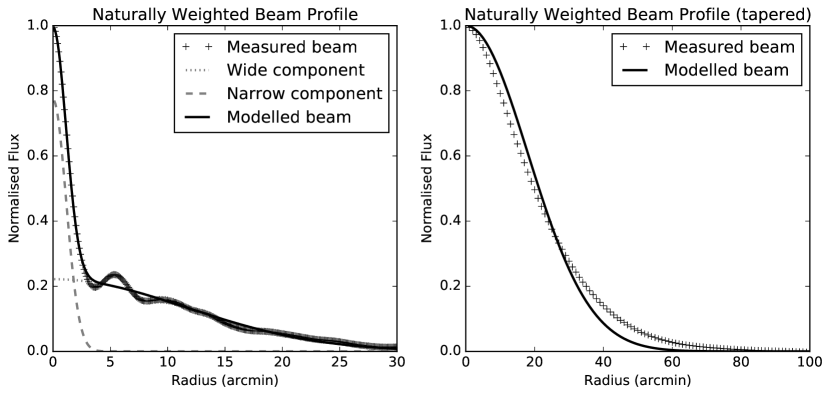
Figure 1: Comparison of naturally weighted synthesized beam without (left) and with (right) $(u,v)$-tapering. The measured synthesized beam in both instances shows the radially averaged profile of the beam. The untapered beam (left) was modelled with a two-component Gaussian; one corresponding to the narrow component and another corresponding to the wide component. The tapered beam (right) was modelled with a single Gaussian component.

Using the rts, calibrated 25$\arcdeg$ wide full Stokes (I, Q, U, and V) dirty image cubes were generated for each snapshot, with 160 kHz frequency channels across the 30.72 MHz band. The images corrected for dipole projection effects and wide-field effects across the entire field-of-view . A sampling of 3 pixels across the naturally-weighted synthesized beam is used in the final imaging. Assuming a receiver temperature of 50 K and a sky temperature of 350 K (Tingay et al., 2013) and taking into consideration the flagging, weighting and baselines used for imaging, we estimate a theoretical sensitivity of 35 mJy beam^-1 (1$\sigma$) per snapshot over the entire 30.72 MHz band at 154 MHz. When combined with all 44 snapshots in our deepest field (epoch 1), this results in a theoretical sensitivity of 5.3 mJy beam^-1. Using the continuum Stokes V image of the deepest field as a guide, we measure an actual image rms of 5.9 mJy beam^-1. Table 2 summarizes the measured continuum image noise and the synthesized beam parameters for all epochs processed in “diffuse” imaging mode. For total intensity, image rms is dominated by classical confusion and sidelobe confusion (Wayth et al., 2015; Franzen et al., 2015); this is also true for the point-source and pulsar imaging presented below. Similarly, for linear polarization, image rms is limited by diffuse polarized structure within the observed field.

Table 2: Summary of measured image noise and synthesized beam characteristics for all epochs and imaging modes. The measured image noise for Stokes I, Q, U and V are listed under columns $\sigma_{i}$, $\sigma_{q}$, $\sigma_{u}$ and $\sigma_{v}$, respectively. In all cases, $\sigma_{i}$ is dominated by classical confusion and sidelobe confusion. For diffuse imaging modes, $\sigma_{q}$ and $\sigma_{u}$ are dominated by diffuse polarized structure in the field. $\theta_{\text{maj}}$ and $\theta_{\text{min}}$ are the major and minor axis of the synthesized beam (FWHM), respectively. PA is the position angle of the synthesized beam measured from north to east.

Epoch	Mode	$\sigma_{i}$	$\sigma_{q}$	$\sigma_{u}$	$\sigma_{v}$	$\theta_{\text{maj}}$	$\theta_{\text{min}}$	PA
		(Jy beam-1)	(Jy beam-1)	(Jy beam-1)	(Jy beam-1)	(arcmin)	(arcmin)	(deg)
1	Diffuse	630	80	102	5.9	$54$	$47$	$-1.8$
1	Point	9.0	3.1	2.4	2.3	$2.4$	$2.2$	$-47$
1	Pulsar	24	1.6	1.5	1.1	$4.6$	$3.8$	$86$
2(a)	Diffuse	690	88	115	39	$54$	$47$	$-1.8$
2(b)	Diffuse	510	240	104	60	$48$	$41$	$11$
2(c)	Diffuse	406	254	140	120	$43$	$37$	$11$
3	Diffuse	600	87	112	6.2	$54$	$47$	$-1.8$
3	Point	11.3	3.0	2.4	2.3	$2.4$	$2.2$	$-47$
3	Pulsar	32	1.4	1.5	1.0	$4.1$	$3.7$	$-89$

Full Stokes dirty image cubes of the inner 400 square degree region of the field were also produced using uniformly weighted images (the restricted field-of-view was due to memory limitations encountered when processing a field at increased resolution). The image cubes are considered “dirty” as no deconvolution was performed. All baselines shorter than 50 $\lambda$ were excluded and no $(u,v)$-tapering was applied. The resulting cubes were better suited for searches of polarized point sources as large-scale emission was effectively filtered out. Table 2 summarizes the measured continuum image noise and the synthesized beam parameters for the two epochs processed in this imaging mode (designated as “point” mode).

Additional targeted imaging was performed in an attempt to detect a known field pulsar, PSR J2330$-$2005 (PSR B2327$-$20), to aid in localizing linearly polarized features. While not ideal, owing to increased sidelobe confusion and PSF structure, natural weighting was used to improve sensitivity. All available baselines were utilized except those below $100\lambda$; these were excluded to limit confusion and contamination from diffuse emission. Full Stokes dirty image cubes of a 16 square degree region centered on the pulsar ($\alpha=23\mbox{${}^{\mathrm{h}}$}30\mbox{${}^{\mathrm{m}}$}26\fs 885$, $\delta=-20\arcdeg 05\arcmin 29\farcs 63$) were produced for epochs 1 and 3. Table 2 summarizes the measured continuum image noise and the synthesized beam parameters for the two epochs processed in this imaging mode (designated as “pulsar” mode).

3 Results

3.1 Total Intensity Continuum Maps

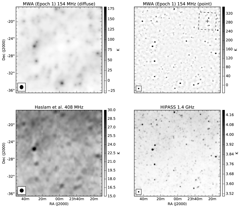
Figure 2: Total intensity maps showing 20$\arcdeg\times 20\arcdeg$ portion of the EoR-0 field. The synthesized beam is shown by the ellipse in the bottom-left corner of each map. [Top Left] Dirty MWA map at 154 MHz optimized for diffuse imaging (naturally weighted and $(u,v)$-tapered). Synthesized beam size is 54$\arcmin\times$47$\arcmin$ FWHM at a position angle of -1.8$\arcdeg$. [Top Right] Dirty MWA map at 154 MHz optimized for point source imaging (uniformly weighted with short baseline cut-off applied). The map has been convolved with a $14.4\arcmin$ FWHM beam to highlight sources. The dashed inset box marks the region imaged in a targeted analysis of PSR J2330$-$2005; the cross marks the location of the pulsar. [Bottom Left] A reprocessed Haslam et al. (1982) 408 MHz map (Remazeilles et al., 2015). Beam FWHM is $51\arcmin$. [Bottom Right] A reprocessed 1.4 GHz HIPASS map (Calabretta et al., 2014). Beam FWHM is $14.4\arcmin$.

The band-averaged epoch 1 total intensity (Stokes I) images optimized for diffuse emission and for point-source analysis are shown in Figure 2. While neither of these images have been deconvolved for the PSF, the beam has been shown to be near-Gaussian and does not significantly degrade the images. To demonstrate that these dirty maps accurately recover diffuse structures, reprocessed 408 MHz Haslam et al. (1982) (Remazeilles et al., 2015) and 1.4 GHz HIPASS (Calabretta et al., 2014) images of the same region have been included in Figure 2 for comparison. The low level diffuse emission observed in the MWA diffuse map correlates well with diffuse emission seen in the Haslam et al. (1982) 408 MHz data and while these features are weaker at 1.4 GHz they are also present in the HIPASS 1.4 GHz data.

3.2 Full Stokes Diffuse Maps

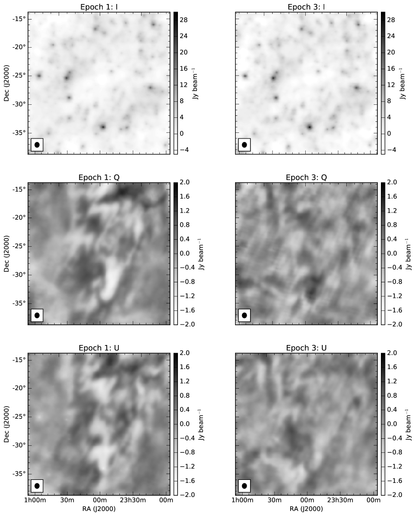
Figure 3: $25\arcdeg\times 25\arcdeg$ Stokes I, Q and U images from deep epoch 1 and epoch 3 data centered on the EoR-0 field. All images are naturally weighted ($(u,v)$-tapered), band-averaged and dirty (not deconvolved). The synthesized beam size is 54$\arcmin\times$47$\arcmin$ FWHM at a position angle of -1.8$\arcdeg$ and is shown by the ellipse in the bottom-left corner of each map. The Stokes I images are highly consistent between epochs but the linear polarization (Stokes Q and Stokes U) are not; this is due to differing ionospheric conditions between the two epochs.

The resulting band-averaged total intensity (Stokes I) and linear polarization (Stokes Q and U) dirty images for the epoch 1 and 3 observations of the EoR-0 field are shown in Figure 3. As no point-source subtraction or peeling (point-source subtraction with direction-dependent calibration) was performed, the Stokes I images are confusion limited and dominated by point sources within the field. Despite the presence of sources with peak brightnesses exceeding 25 Jy beam^-1 in total intensity, the linear polarization maps contain mostly smooth features and these are uncorrelated with features in Stokes I. A few of the brightest sources are just perceptible in the polarization maps at about the $1\%$ level but do not affect the overall structure of the diffuse emission seen in those maps. The Q and U maps are mostly dominated by smooth extended structures ranging from $1\arcdeg$ to $8\arcdeg$ in extent and filament-like features, a number of which are approximately aligned in a north-west direction. Note that while the Stokes I maps are virtually identical in epoch 1 and 3, the Stokes Q and U maps are quite different. In particular, the epoch 3 U image appears to exhibit features found in the epoch 1 Q image and the epoch 3 Q image appears to have inverted features from the epoch 1 U image. The changes observed between the epochs appear consistent with a rotation in the Q$-$U plane. As will be shown in Section 3.4, these changes are a result of ionospheric Faraday rotation.

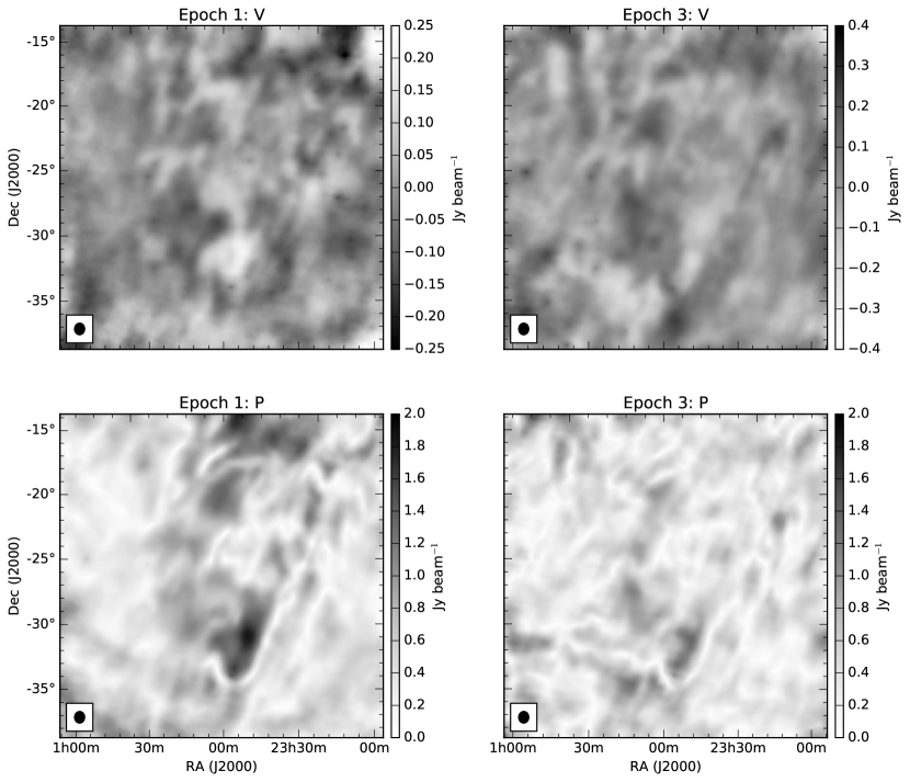
Figure 4: Circular polarization (Stokes V) and polarized intensity (P) images. Image details are as for Figure 3, but the intensity scales of the Stokes V images have been adjusted to highlight the leakage seen from Stokes U. The polarized intensity images do not show consistent structure as a result of differing ionospheric conditions between the two epochs.

For comparison and diagnostic purposes, the band-averaged circular polarization (Stokes V) and polarized intensity (P) images are shown for epochs 1 and 3 in Figure 4. The circular polarization maps clearly exhibit leakage from Stokes U into Stokes V at the $\sim$$10\%$ level in epoch 1 and $\sim$$20\%$ level in epoch 3; due to a combination of frequency-dependent XY phase errors that have not been accounted for and uncertainties in the beam model. We note that this is relatively high but even if corrected for, the improvement in Stokes U would only be at a level that is already dominated by existing errors associated with the PSF and sidelobe confusion. We also note that the leakage from Stokes U to Stokes V is not prominent in the uniformly weighted image used for point source analysis; because the point sources are significantly weaker in Stokes U compared to the diffuse emission and so any leakage would be below the Stokes V noise level.

Comparing the polarized intensity images between epoch 1 and 3, one would expect that the images should remain constant between epochs. However, there are clear differences between the two. The epoch 1 image has significantly brighter structures whereas the epoch 3 image does not. These differences are caused by significantly different ionospheric conditions between the two epochs resulting in different levels of depolarization in the band-averaged Q and U images used to form the polarized intensity images. The polarized intensity image from epoch 1 is dominated by a large ($\sim$$4\arcdeg\times 7\arcdeg$) and bright feature (peaking at $\sim$$1.8$ Jy beam^-1) centered around $\alpha=23\mbox{${}^{\mathrm{h}}$}50\mbox{${}^{\mathrm{m}}$}$, $\delta=-31\arcdeg$. Depolarization canals, unresolved regions with little or no emission in linear polarization, are further clearly visible; many of them laying preferentially in a north-west orientation. The most prominent depolarization canals appear to be associated with the bright extended feature. In particular, one curves around the lower extent of the feature (starting around $\alpha=0\mbox{${}^{\mathrm{h}}$}$, $\delta=-35\arcdeg$) and then extends linearly towards the north-west edge of the field (through $\alpha=23\mbox{${}^{\mathrm{h}}$}30\mbox{${}^{\mathrm{m}}$}$, $\delta=-25\arcdeg$).

3.3 Rotation Measure Synthesis

When propagating through a magnetized plasma, a linearly polarized signal undergoes Faraday rotation. The effect is particularly pronounced at long wavelengths as the magnitude of rotation is proportional to the wavelength squared:

$$\chi(\lambda^{2})=\chi_{0}+\phi\lambda^{2}$$ (1)

where $\chi(\lambda^{2})$ is the measured linear polarization angle (rad) at wavelength $\lambda$ (m), $\chi_{0}$ is the intrinsic polarization angle (rad) and the overall strength of the effect is characterized by the Faraday depth $\phi$ (rad m^-2). The Faraday depth along the sightline to a source is defined as (Burn, 1966):

$$\phi(d)=0.81\int_{d}^{0}n_{e}B_{\parallel}\cdot dl\,,$$ (2)

where $n_{e}$ is the electron density (cm^-3) and $B_{\parallel}$ is the magnetic field component parallel to the line of sight ($\mu$G). The integral is performed along the line of sight (of which $dl$ is the differential element) from the observer to a distance $d$ (pc). If Faraday rotation is not taken into consideration at long wavelengths, sources at any appreciable Faraday depth will depolarize over the available observing band, an effect known as bandwidth depolarization.

Rotation Measure (RM) synthesis (Brentjens & de Bruyn, 2005) is a technique that takes advantage of the Fourier relationship between the complex polarized intensity as a function of wavelength squared, $P(\lambda^{2})=Q(\lambda^{2})+iU(\lambda^{2})$, and the Faraday dispersion function (FDF) $F(\phi)$ which is the polarized intensity as a function of Faraday depth (Burn, 1966), i.e.

$$P(\lambda^{2})=W(\lambda^{2})\int_{-\infty}^{+\infty}F(\phi)e^{2i\phi\lambda^{2}}\text{d}\phi$$ (3)

where $W(\lambda^{2})$ is a weighting function and $\phi$ is the Faraday depth. RM synthesis reconstructs the Faraday dispersion function $F(\phi)$ from an irregularly sampled $P(\lambda^{2})$. The rotation measure spread function (RMSF), which is the Faraday depth equivalent of the point spread function, is the Fourier transform of the weighting function and depends on bandwidth, channel weighting and wavelength.

In general, frequency channels may be weighted by $W(\lambda^{2})$ to account for varying sensitivity across the band. However, measuring the Q and U image noise in the presence of large-scale structures that vary dramatically as a function of frequency is problematic. To simplify processing, we have weighted all frequency channels in the image cubes equally, i.e. $W(\lambda^{2})=1$. We anticipate only a slight loss in overall sensitivity resulting from this choice of weighting scheme as the observed sensitivity across the band is relatively smooth when measured in uniformly weighted images. Using definitions from Brentjens & de Bruyn (2005), for the 154 MHz band with 160 kHz channels, the resulting RMSF provides a resolution of $\delta\phi$=2.3 rad m^-2, maximum-scale size sensitivity of 1.0 rad m^-2 and Faraday depth range of $\lvert\phi_{max}\rvert$=160 rad m^-2. As the maximum-scale size is smaller than the resolution $\delta\phi$, these observations cannot resolve Faraday thick structures.

The incomplete sampling available in $\lambda^{2}$ results in side-lobes at about the $10\%$ level in the RMSF. These have been accounted for by using the RM clean algorithm, as described by Heald (2009). In summary, the RM clean algorithm deconvolves peaks in Faraday space with the RMSF to determine the location and amplitude of clean components. The resulting clean components are then convolved with a Gaussian restoring function that has a FWHM equivalent to the RMSF resolution (i.e. $\delta\phi$=2.3 rad m^-2).

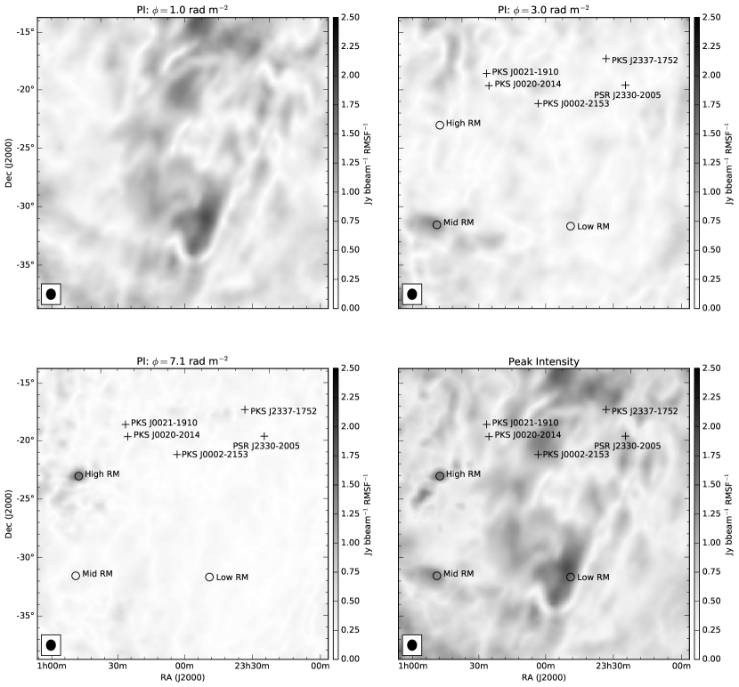
Figure 5: Polarized features observed at three Faraday depths in epoch 1 data taken from the RM cleaned cube (corrected for ionospheric Faraday rotation). The RMSF has a FWHM of 2.3 rad m^-2. [Top Left] $\phi=+1.0$ rad m^-2. [Top Right] $\phi=+3.0$ rad m^-2. [Bottom Left] $\phi=+7.1$ rad m^-2. [Bottom Right] Peak intensities in the Faraday depth spectra at each spatial pixel. The flux scale is in Jy beam^-1 RMSF^-1. The synthesized beam, shown as a filled ellipse, is 54$\arcmin\times$47$\arcmin$ FWHM at a position angle of -1.8$\arcdeg$. Circles mark the locations of diffuse features referred to in the text. Crosses mark locations of polarized point sources detected in high resolution imaging; these sources are not visible in the low resolution images as they are dominated by the presence of large-scale structure.

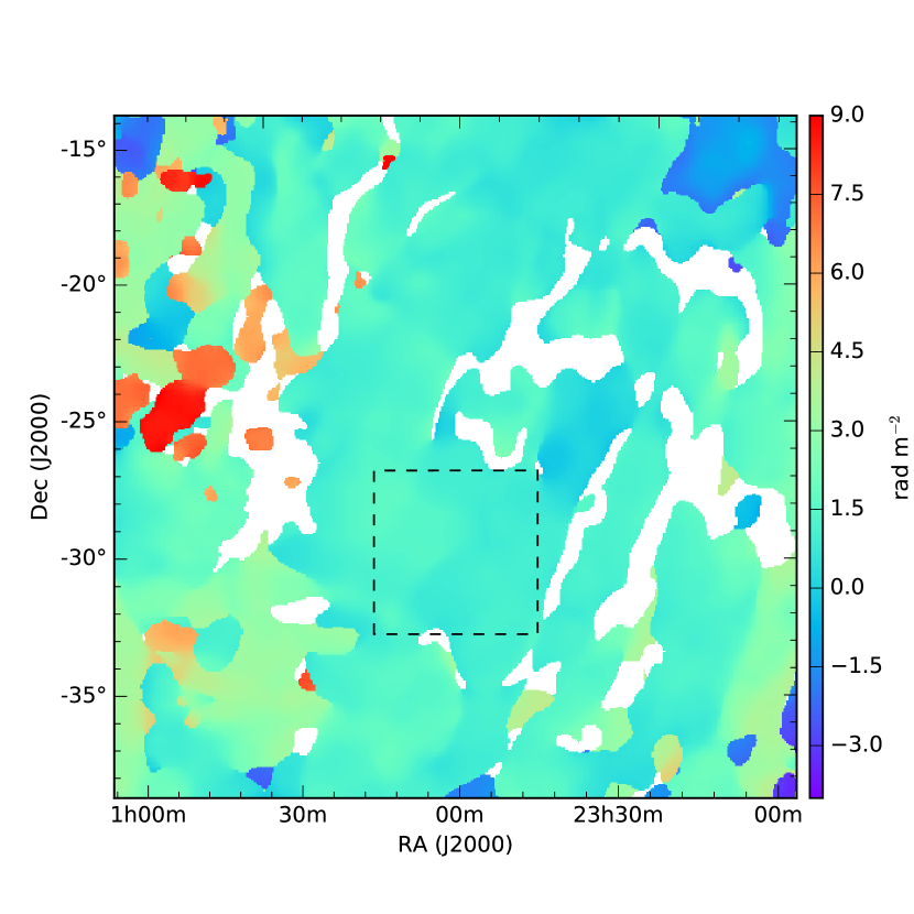
Figure 6: Faraday depth measure at peak polarized intensity for each pixel in the Faraday depth cube (corrected for ionospheric Faraday rotation). Regions with low signal to noise have been blanked out. The Faraday depth is measured in rad m^-2. The $6\arcdeg\times 6\arcdeg$ dashed square shows the extent of a region containing both smooth Faraday depth variations and high levels of polarized intensity.

Figure 5 highlights features observed in Faraday space at three different Faraday depths ($+1.0$ rad m^-2, $+3.0$ rad m^-2 and $+7.1$ rad m^-2) in the epoch 1 data. The vast majority of the diffuse structure appears at low Faraday depths ($\sim$$1$ rad m^-2) and is dominated by a bright extended feature (labelled “Low RM”) that was noted in the epoch 1 polarized intensity map (see Figure 4). Depolarization canals also dominate the entire field-of-view at this Faraday depth with several of the more significant canals oriented in an approximately SE$-$NW alignment. At a Faraday depth of $+3.0$ rad m^-2 the bulk of the features seen at $+1.0$ rad m^-2 are gone and are replaced by a number of $\sim$$2\arcdeg-4\arcdeg$ wide structures in the SE corner of the EoR-0 field (the brightest of which is labelled “Mid RM”). At $+7.1$ rad m^-2, a small, barely resolved, feature is seen to the east (labelled as “High RM”). Just SE of this source is a slightly more extended component that peaks at $\sim$$+9$ rad m^-2. The mid-to-high RM features may be associated with the increased level of diffuse polarized emission observed by Bernardi et al. (2013) towards the south Galactic pole at similar Faraday depths. Figure 6 shows the Faraday depth at peak emission in the Faraday depth cube for each line of sight in the field. The figures show that the majority of the EoR-0 field is dominated by features at low Faraday depths and that these features vary quite smoothly across the field. Apart from the small number of sources already described at higher Faraday depths, there are a number of weak features at negative Faraday depths near the edge of the field; these are not likely to be associated with real features and are caused by a combination of decreased sensitivity at the edge of the field and sidelobe structures contaminating the field at low signal to noise.

The deconvolved Faraday dispersion functions for the samples taken in the low and high RM regions are shown in Figure 7. The residual rms is 16 mJy beam^-1 RMSF^-1, 42 mJy beam^-1 RMSF^-1 and 29 mJy beam^-1 RMSF^-1 for the low, mid and high RM sources, respectively. The high RM FDF appears to contain more than one peak: a main peak at $\phi=+7.2$ rad m^-2, an intermediate 530 mJy beam^-1 RMSF^-1 peak at $\phi=+3.5$ rad m^-2 and a 230 mJy beam^-1 RMSF^-1 peak at $\phi=+0.7$ rad m^-2. The additional minor peaks in the high RM FDF fluctuate between epoch 1 and 3 and are due to side lobe contamination which introduces frequency dependent structure into the Faraday spectra that is also time dependent.

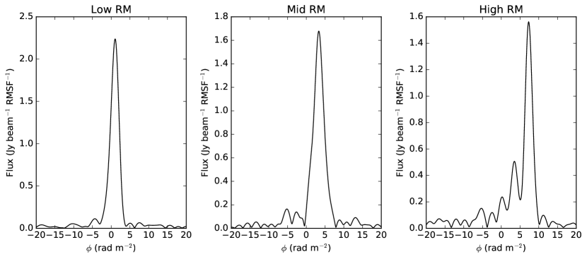
Figure 7: Sample Faraday dispersion functions (corrected for ionospheric Faraday rotation) shown for the low ($\phi=+1.0$ rad m^-2), medium ($\phi=+3.0$ rad m^-2) and high ($\phi=+7.1$ rad m^-2) RM features highlighted in Figure 5. The three Faraday dispersion functions shown here correspond to the three peaks visible in the RM distribution plot shown in Figure 8. No features above the noise floor are seen outside of the Faraday range shown here. The Faraday dispersion functions were deconvolved with rmclean (Heald, 2009).

3.4 RM distribution and Ionospheric Faraday Rotation

The ionosphere affects observations through positional shifts of background sources and through Faraday rotation of linearly polarized signals. A gradient in total electron content (TEC) of the ionosphere across the field-of-view will result in positional shifts of sources; this has been observed previously with the MWA and studied in detail (Loi et al., 2015a, b, c). For diffuse polarization the effect is an order of magnitude smaller than the size of the features being studied and can safely be ignored.

The absolute TEC, in combination with the magnetic field in the direction being observed, can measurably contribute to the observed RM of a background source. The TEC at a given time, from a given location on the Earth, observed towards a particular line of sight, can be estimated based on Global Positioning System (GPS) models (Arora et al., 2015). Using the TEC estimated by these models in combination with terrestrial magnetic field models, the predicted ionospheric component of Faraday rotation may be determined. An implementation of these models can be found in the albus (Willis et al., 2016) package. We used albus to determine the mean Faraday rotation introduced as a result of the ionosphere during the course of the epoch 1 observation and estimated it to be $-0.7\pm 0.2$ rad m^-2. When corrected for ionospheric Faraday rotation, the distribution of RM in the EoR-0 field peaks at 1.0 rad m^-2 with a standard deviation of $\sigma_{\phi}=0.34$ rad m^-2; see Figure 8. A few further sub-peaks are seen within this distribution but the vast majority of features are contained within $-2<\phi<+10$ rad m^-2.

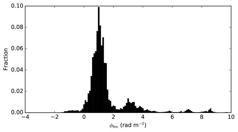
Figure 8: Distribution of rotation measures in the EoR-0 field after ionospheric correction and performing rmclean to remove sidelobes in Faraday space. The binning width is 0.1 rad m^-2. The main peak of the distribution is at 1.0 rad m^-2. Sub-peaks in the distribution are due to features present at higher Faraday depths.

When images are compared across the three epochs at 154 MHz, the total intensity maps remain unchanged. However, there are clear differences in the linear polarization maps, particularly between epoch 1 and the two subsequent epochs. Using RM synthesis and searching for peak emission in Faraday depth for each line of sight revealed that all of the observed structures were consistent between the epochs but that they had been shifted in Faraday space. This is shown in Figure 9 for the epoch 1 and epoch 3 data; here the peak intensity maps are consistent but the peak emission occurs at $+0.3$ rad m^-2 in epoch 1 and at $\phi=-1.2$ rad m^-2 in epoch 3. Both albus (Willis et al., 2016) and ionfr (Sotomayor-Beltran et al., 2013) predict a shift in the ionospheric component of $\sim$$-1.5$ rad m^-2 in Faraday rotation from epoch 1 to epoch 3 (ionospheric RM of $-0.7$ rad m^-2 for epoch 1 and $-2.2$ rad m^-2 for epoch 3). When these shifts are applied to the Faraday depth cubes, the peak emission for both epochs occurs at $\sim$$1.0$ rad m^-2, verifying that the shift is associated with the ionosphere and not caused by variability or the instrument. This highlights the need for a correction to mitigate the effects of ionospheric Faraday rotation. However, it also demonstrates that the ionosphere is quite stable as a function of time and direction over the MWA field-of-view and that, to first order, a single shift in Faraday depth (as opposed to a grid of multiple direction dependent shifts) is sufficient to correct for these ionospheric effects.

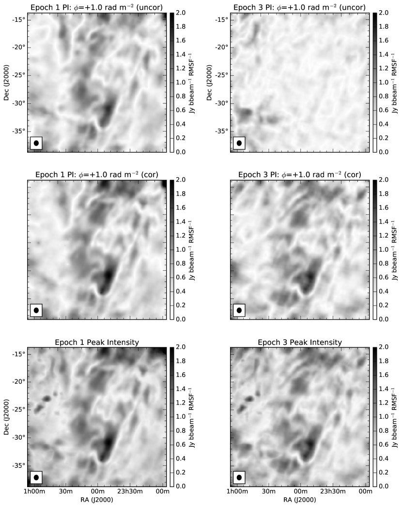
Figure 9: Effect of ionospheric Faraday rotation on diffuse polarization as observed in epochs 1 and 3. Top: Polarized intensity at $\phi=+1.0$ rad m^-2 before correcting for ionospheric Faraday rotation. Center: Polarized intensity at $\phi=+1.0$ rad m^-2 after correcting for ionospheric Faraday rotation. Bottom: Peak intensity in the Faraday spectra at each spatial pixel. albus reports an ionospheric Faraday rotation of $-0.7$ rad m^-2 in epoch 1 and $-2.2$ rad m^-2 in epoch 3. Differences observed near the edge of the field between the two epochs after ionospheric correction are due to primary beam errors and sidelobe confusion.

An interesting possibility with the MWA, given the high sensitivity to diffuse structures that the instrument provides, is to use the diffuse polarized background to track and measure the influence of ionospheric and heliospheric Faraday rotation. An estimate of the ionosphere-corrected Faraday rotation towards a source of bright diffuse emission ($\phi_{src}$) can be determined by performing a least-squares fit that minimizes $\phi_{src}-(\phi_{obs}-\phi_{ALBUS})$ over multiple observing snapshots and/or epochs, where $\phi_{obs}$ is the observed Faraday rotation towards the source and $\phi_{ALBUS}$ is the estimated ionospheric Faraday rotation at the time of the observation. By observing over multiple epochs, to overcome the relatively large errors associated with individual predictions of $\phi_{ALBUS}$, the overall error in $\phi_{src}$ can be minimized. Once an estimate of the ionosphere-corrected Faraday rotation is established, it can be used to estimate the ionospheric component of Faraday rotation at that source location at any epoch. Using this approach for all available snapshots in each of the three epochs, the fit to $\phi_{src}$ of the high RM source (see Figure 5) was determined to be $\phi_{src}=7.20\pm 0.01$ rad m^-2. Figure 10 plots the ionospheric component ($\phi_{obs}-\phi_{src}$) at the high RM source location for each snapshot and epoch. The measured component tracks both predictive models quite well from epoch to epoch and even from snapshot to snapshot. This demonstrates that observations of diffuse polarization may allow the effects of the ionosphere to effectively be calibrated in fields where the RM structure has been previously determined, without the need to resort to predictive models. The technique also has the potential to aid ionospheric studies by mapping ionospheric changes both temporally and spatially over a wide field-of-view. In combination with predictive models, this technique may also provide a means to detect and track the propagation of space weather events, as caused by coronal mass ejections or solar flares, by observing the shift they impart on the RM signature of the diffuse polarized background (Oberoi & Kasper, 2004).

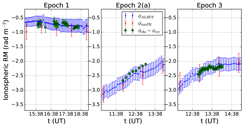
Figure 10: Measurements of ionospheric Faraday rotation ($\phi_{obs}$ is the observed Faraday rotation of a source and $\phi_{src}$ is the previously determined ionosphere-corrected Faraday rotation of the source) at the position of the high RM feature shown in Figure 5 for each observed snapshot and epoch (green points). The blue and red points are the predicted components of ionospheric Faraday rotation from albus ($\phi_{ALBUS}$) and ionfr ($\phi_{ionFR}$), respectively. Note that an additional seven 2 minute snapshots from epoch 2(a) were used here to track the high RM feature as it drifted through the zenith-pointed beam of that observation, however those snapshots were not used in subsequent processing as the bulk of the EoR-0 field had already drifted out of the field-of-view.

3.5 Gradient maps

To examine filamentary magnetized structures believed to result from turbulence in the local interstellar medium Burkhart et al. (2012), polarization gradient maps of the Stokes vector (Q and U) were formed using the method described by Gaensler et al. (2011). The polarization gradient function is defined as:

$$\lvert\mathbf{\nabla P}\rvert=\sqrt{\left(\frac{\partial Q}{\partial x}\right)^{2}+\left(\frac{\partial U}{\partial x}\right)^{2}+\left(\frac{\partial Q}{\partial y}\right)^{2}+\left(\frac{\partial U}{\partial y}\right)^{2}}\,.$$ (4)

Time-dependent effects were examined by comparing changes in the gradient map from snapshot to snapshot and against the time-averaged data set. Figure 11 shows gradient maps from the epoch 1 observation using a single 112 s snapshot compared against a gradient map using all of the available data from that epoch. When corrected for ionospheric effects, the structures seen in these gradient maps are centered at a Faraday depth of $+1.0$ rad m^-2 as this is where the bulk of the polarized emission exists (see Figure 8).

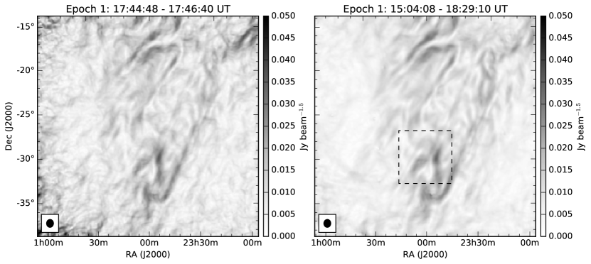
Figure 11: Left: An ionosphere-corrected polarization gradient map from a single 112 s snapshot of epoch 1 data. Right: The ionosphere-corrected polarization gradient map derived from time-averaged epoch 1 data ($44\times 112$ s snapshots). Units are in Jy beam^-1.5. The $6\arcdeg\times 6\arcdeg$ dashed square shows the extent of a region containing both smooth Faraday depth variations and high levels of polarized intensity.

The most prominent features in Figure 11 remain stable as a function of time. Minor changes can be seen in the fainter structures and these are primarily due to a combination of image noise; sidelobe confusion; and errors associated with incomplete $(u,v)$ sampling. We note that the first few snapshots of epoch 1 are detrimentally affected by the presence of the Galactic plane within a far sidelobe as this epoch included low elevation beam-former pointings that were not used in the epoch 2 or epoch 3 data. The projected baselines of the MWA are severely foreshortened for sources at low elevation and the array is particularly sensitive to bright and extended sources in those locations (Thyagarajan et al., 2015). Nonetheless, when integrating data over a wide range of hour angles, the source sidelobe effects are diluted and the exclusion of the affected snapshots has a minimal impact on the final integrated gradient map. Gradient maps were also produced for the remaining epochs at 154 MHz but no significant changes were observed once the maps were corrected for ionospheric Faraday rotation.

To examine the evolution of gradient map features as a function of observing frequency, gradient maps were created for the three GLEAM bands, i.e. epochs 2(a), 2(b) and 2(c). The EoR-0 field was only fully visible in the first snapshot of the epoch 2 data as the Sun was in the process of setting just as the field was passing through zenith. As such, the sensitivity is limited to that of a single snapshot in these data. Figure 12 shows the resulting gradient maps for each band of epoch 2 data, with channels across each 30.72 MHz band averaged to increase signal to noise. The point-like sources that begin to appear in epoch 2(b) and dominate in epoch 2(c), result from apparent polarization leakage from bright Stokes I sources. The level of leakage increases with frequency and angular distance from zenith. For the most part, this leakage is due to errors in the primary beam model and will be reduced once improved beam models are implemented into the imaging pipeline (Sutinjo et al., 2015). The leakage in epoch 2(a) is minimal as this is where the beam model and instrument were designed to perform optimally; thus its behaviour is well-defined. Increased noise levels are also evident at the edge of the field in the higher frequency bands as a result of the decreased field-of-view available in those bands.

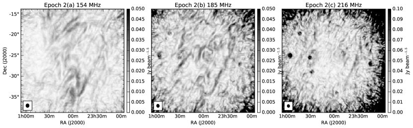
Figure 12: Gradient maps from ionosphere-corrected epoch 2 data of the EoR-0 field in three available frequency bands: 154 MHz (left), 185 MHz (center) and 216 MHz (right). Clear evidence of polarization leakage, primarily contamination from Stokes I point sources, is seen in the higher frequency bands where beam model errors are more apparent. The available field-of-view also decreases as a function of increasing frequency and so the higher frequency maps exhibit increased levels of noise at the edge of the field.

Comparing the gradient maps in the three different bands, the dominant features are stationary with respect to spatial coordinates in the epoch 2(a) and 2(b) images. Some features, such as the linear feature that runs from NW to SE near the western edge, remain persistent over all three of the bands. The weaker structures are more difficult to trace, particularly in epoch 2(c), as a result of the poor sensitivity available in a single snapshot and systematic issues associated with the beam, noise and available field-of-view.

[controls,width=]25f13_0023

Figure 13: Epoch 1 EoR-0 gradient maps for 24 $\times$ 1.28 MHz channels across the 154 MHz band. Note that Adobe Acrobat Reader is required to view the animated gradient map cube shown here.

An alternative view of the frequency dependent behaviour of the polarized gradients in the field can be obtained from the deep epoch 1 EoR-0 observations, albeit over the limited range of frequencies available in that observation ($138.88$–$169.60$ MHz). The epoch 1 data provide sufficient sensitivity, as a result of the longer tracking observation available, to study the polarization gradient evolution on a per-160 kHz channel basis. Figure 13 presents an animation of the gradient map as a function of frequency across the 30.72 MHz band of the 154 MHz epoch 1 observations; in this animation, subsets of $6\times 160$ kHz channels have been frequency-averaged to form a smaller number of 1.28 MHz channels. The polarized gradients are now more prominent in each of the frequency channels and can be seen to vary smoothly in intensity as a function of frequency but show no significant spatial movement. In general, once features appear at lower frequencies, they continue to persist up to the higher frequency gradient maps. For example, the gradient around the bright polarized feature labelled ”Low RM” in Figure 5 persists over the entire band. However, an SE to NW gradient appears towards the east and west only in the upper portion of the band. Similarly, features in the northern part of the image, some forming loop-like structures, also only appear in the upper end of the band.

3.6 Polarized point sources

The uniformly weighted polarization image cubes generated using all of the longest MWA baselines are well suited for the detection of polarized point sources. An initial inspection of the RM cube, created using the uniformly weighted Stokes Q and U cubes, reveals a clear detection of the extragalactic source PKS J0021$-$1910 (PKS B0018$-$194). A cut-out image for the source and its associated Faraday dispersion function are shown in Figure 14 and Figure 15, respectively. In the uncorrected epoch 3 data the source has an RM of $+5.6$ rad m^-2 and is detected with a signal to noise of 10 in each snapshot. When corrected for ionospheric effects using albus predictions of the ionospheric Faraday rotation, a fit of $\phi=+7.8\pm 0.1$ rad m^-2 is obtained for this source. With a total intensity of 4.7 Jy beam^-1 and a polarized intensity of 140 mJy beam^-1, the source is 3.0% polarized. The polarimetric characteristics of the source are consistent with a measurement made at 1.4 GHz, RM $=3.6\pm 5.2$ rad m^-2 and 3.67% polarization (Taylor et al., 2009).

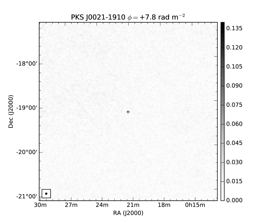
Figure 14: Cut-out showing the polarized source PKS J0021$-$1910. The synthesized beam is 2.2′$\times$2.4′FWHM with a position angle of -47°.

A subsequent search was performed concentrating on the locations of known polarized sources, using the Taylor et al. (2009) catalogue as a reference. The catalogue contains 399 polarized sources within the 400 sq. degree region imaged around the EoR-0 field. We use a conservative 14$\sigma$ cut-off in the time-averaged data cube to ensure that spurious detections are not made as a result of polarization leakage from bright Stokes I sources and the associated sidelobe structure this leakage introduces into the Faraday spectra. Any sources with $\lvert\text{RM}\rvert<1$ rad m^-2 were also filtered out; as these would most likely trigger false-positives as a result of polarization leakage. In all, two sources were detected: PKS 0002$-$2153 (PKS B2359$-$221) and PKS J0021$-$1910 (PKS B0018$-$194). The Faraday dispersion functions for these sources are shown in Figure 15.

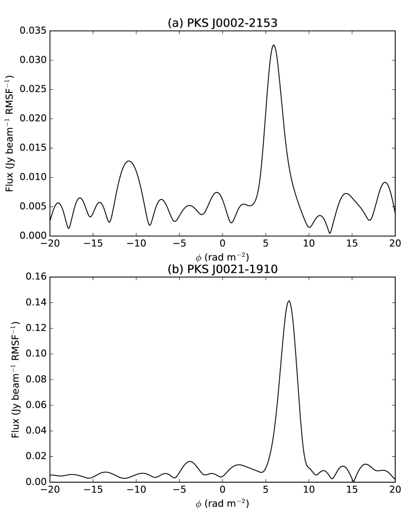
Figure 15: Sources detected with high-resolution imaging. (a) Faraday dispersion function for PKS J0002$-$2153. RM$=+5.7$ rad m^-2. Noise is 2.5 mJy beam^-1 RMSF^-1 rms. (b) Faraday dispersion function for PKS J0021$-$1910. RM$=+7.8$ rad m^-2. Noise is 3.1 mJy beam^-1 RMSF^-1 rms.

Since deep observations were made at two epochs, a further test of the sources was made by checking whether their RMs were shifted in Faraday space by an amount that was consistent with the expected shift caused by the different ionospheric conditions between the two epochs. The advantage of this method is that it can identify real sources that were confused with instrumental leakage, because in at least one of the epochs, such a source would be shifted sufficiently away from RM$=0.0$ rad m^-2 to allow a positive identification. All of the previously detected sources were verified using this method and two additional sources were also identified: PKS J2337$-$1752 (PKS B2335$-$181) and PKS J0020$-$2014 (PKS B0017$-$205). Figures 16(a) and 16(c) show the RM synthesis components detected in epochs 1 and 3. In epoch 1 the instrumental component and the source components are confused near RM=0.0 rad m^-2 for both PKS J0020$-$2014 and PKS J2337$-$1752. In epoch 3, the ionosphere clearly shifts the source RM away from the instrumental component, thus enabling a positive identification. The Faraday dispersion functions for these two sources are shown in Figure 16.

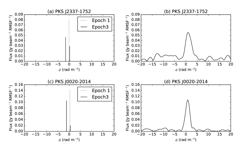
Figure 16: Sources found in a multi-epoch analysis that distinguishes real sources from instrumental effects by searching for peaks shifted in Faraday space as a result of ionospheric Faraday rotation. (a) Peaks detected in RM synthesis in epochs 1 and 3 for PKS J2337$-$1752 before correcting for the effects of ionospheric Faraday rotation. (b) Faraday dispersion function for PKS J2337$-$1752 in epoch 3 after correcting for the effects of ionospheric Faraday rotation. RM$=+0.8$ rad m^-2. Noise is 3.9 mJy beam^-1 RMSF^-1 rms. (c) Peaks detected in RM synthesis in epochs 1 and 3 for PKS J0020$-$2014 before correcting for the effects of ionospheric Faraday rotation. (d) Faraday dispersion function for PKS J0020$-$2014 in epoch 3 after correcting for the effects of ionospheric Faraday rotation. RM$=+1.0$ rad m^-2. Noise is 3.4 mJy beam^-1 RMSF^-1 rms.

The parameters associated with all detected point sources are summarized in Table 3. All but PKS J2337$-$1752 have RMs consistent with those measured by Taylor et al. (2009). Not all of the sources appear to have been significantly depolarized at MWA wavelengths compared to observations at 1.4 GHz, which suggests that there is not a systematic reason to explain the overall small number of detections. The two most highly polarized extragalactic sources, PKS J0020$-$2014 and PKS J0021$-$1910, are also the two largest sources in spatial extent amongst our detected sources. PKS J0020$-$2014 is a giant radio galaxy with a redshift of $z=0.197$ (Ishwara-Chandra & Saikia, 1999) and an extent of 1.22 Mpc, while PKS J0021$-$1910 is a known double radio source with a redshift of $z=0.0952$ and an extent of 270 kpc (Reid et al., 1999). The remaining sources are all relatively compact.

The pulsar PSR J2330$-$2005 does not appear in the Taylor et al. (2009) catalogue and is not detected in the uniformly weighted MWA data. It is, however, detected in both circular and linear polarization and in both epochs in the targeted search, using naturally-weighted data with short baselines removed (to avoid confusion from the diffuse structures). The parameters associated with the pulsar are summarized in Table 3 and the Faraday dispersion function is shown in Figure 17. The secondary peaks in the Faraday dispersion function for the pulsar are unlikely to be real - most likely they are due to a combination of thermal noise and sidelobe noise as a result of the complicated PSF beam shape that results from natural weighting. In circular polarization, we measure a total flux for the pulsar at 154 MHz of $8.9\pm 1.1$ mJy in epoch 1 and $9.6\pm 1.0$ mJy in epoch 3. We estimate a fractional circular polarization of $\sim$$7\%$ based on the total intensity of 140 mJy measured at the pulsar position; however, the field is highly confused in total intensity at this level. As such, the total intensity is most likely over-estimated and the fractional polarization is thus a lower limit. This would be consistent with the $22\%$ circular polarization observed in the integrated pulse profile of the pulsar at 648 MHz (McCulloch et al., 1978) .

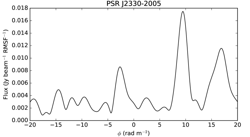
Figure 17: Faraday dispersion function for PSR J2330$-$2005 from epoch 1 after correcting for the effects of ionospheric Faraday rotation. RM$=+9.6$ rad m^-2. Noise is 1 mJy beam^-1 RMSF^-1 rms.

Offringa et al. (2016) performed a deep point-source survey of the EoR-0 field using 45 hours of MWA data and achieved a sensitivity of 0.6 mJy beam^-1 in polarization. Using a novel peeling algorithm, spectra for the 586 brightest sources in the field were presented. Unfortunately, PKS J0020$-$0014 is a resolved source and so was discarded from the catalogue and PSR J2330$-$2005 fell outside of the restricted field-of-view of the survey. PKS J0021$-$1910 appears in the catalogue but is not detected in polarization. The Offringa et al. (2016) survey did not consider Faraday rotation of the source and so linearly polarized sources with non-zero RM are depolarized. In addition, when combining results from multiple epochs, ionospheric Faraday rotation was also not considered; this too would lead to depolarization of linearly polarized sources (a similar issue was encountered by Moore et al. 2016 in PAPER observations). It is thus not surprising that linearly polarized sources were not detected by Offringa et al. (2016), but circularly polarized sources should not be as greatly affected when combining data from multiple epochs. Indeed, on closer inspection, PSR J2330$-$2005 is detected in the Offringa et al. (2016) data at the $6.3\%$ level with a circularly polarized flux density of $6.5$ mJy (Offringa, private communication).

Table 3: Details of polarized point sources detected in the EoR-0 field. RM${}_{\text{MWA}}$ is the rotation measure determined from MWA observations (corrected for ionospheric Faraday rotation). RM${}_{\text{lit}}$ is the rotation measure in literature. P${}_{\text{MWA}}$ and p_MWA are the polarized flux density and fraction polarization derived from MWA observations, respectively. p${}_{\text{lit}}$ is the fractional polarization in literature, at an observing frequency of $\nu_{\text{obs}}$. $\text{DP}(1400,154)$ is the depolarization ratio from 1.4 GHz to 154 MHz.

Source	RM${}_{\text{MWA}}$	RM${}_{\text{lit}}$	P${}_{\text{MWA}}$	pMWA	p${}_{\text{lit}}$	$\nu_{\text{obs}}$	$\text{DP}(1400,154)$
	(rad m-2)	(rad m-2)	(mJy beam-1)			(MHz)
PSR J2330$-$2005	$+9.6\pm 0.1$	$+16\pm 3$ a	19	14%	16%	648 b
		$+9.5\pm 0.2$ a
		$+9.5\pm 0.6$ c
PKS J2337$-$1752	$+0.6\pm 0.1$	$+12.2\pm 1.3$ d	46	1.3%	$3.67\pm 0.07$%	1400 d	0.26
PKS J0002$-$2153	$+5.8\pm 0.1$	$+6.0\pm 4.9$ d	33	2.1%	$6.0\pm 4.9$%	1400 d	0.32
PKS J0020$-$2014	$+1.6\pm 0.1$	$+1.5\pm 2.7$ d	105	3.5%	$12\pm 1.3$%	1400 d	0.37
PKS J0021$-$1910	$+7.9\pm 0.1$	$+3.6\pm 5.2$ d	140	3.0%	$3.6\pm 5.2$%	1400 d	0.91
a Hamilton & Lyne (1987);b McCulloch et al. (1978); c Johnston et al. (2007); d Taylor et al. (2009)

4 Discussion

4.1 Size-scale of Structures in Linearly Polarized Emission

The linearly polarized features seen in Figure 3 are highly prominent even in single 112 s snapshot images. The LOFAR observations differ from the MWA observations in that they incorporate longer baselines, are at lower Galactic latitudes and their imaging utilizes a robust image weighting of 0 which results in higher resolution ($\sim$$3\arcmin$–$4\arcmin$) images compared to the $\sim$$50\arcmin$ naturally-weighted and $(u,v)$-tapered images of the MWA presented here. Factoring in the beam size, the Jelić et al. (2014) LOFAR observations have a sensitivity of $\sim$$650$ mK at the $\sim$$4\arcmin$ scale, whereas the MWA epoch 1 observations have a sensitivity of $\sim$$33$ mK at the $\sim$$50\arcmin$ scale.

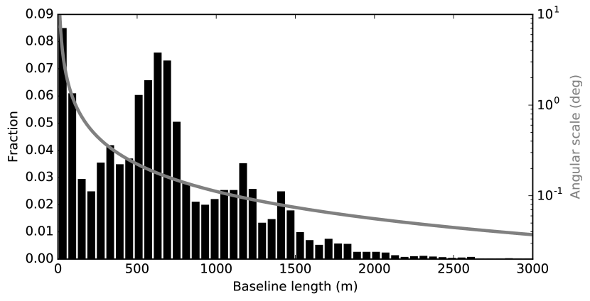
Figure 18: Snapshot imaging baseline distribution for MWA 128T when observing at zenith ($\delta=-26.7\arcdeg$). The grey curve plots the angular scale probed as a function of baseline length.

The unique baseline distribution and radio quiet location of the MRO (Offringa et al., 2015) give excellent sensitivity to structures $1\arcdeg-10\arcdeg$ in extent and sample a region not accessible to other low frequency instruments such as LOFAR (van Haarlem et al., 2013), for example. While the 128 tiles of the MWA provide a total of 8128 baselines out to almost 3 km, the peak sensitivity of the array is derived from its dense inner core which was specifically designed for EoR science. Figure 18 shows the fraction of baselines as a function of baseline length. Approximately 8.5% of the available baselines (689) are shorter than 60 m and nearly 15% (1183) are shorter than 120 m. The combination of sensitivity to large-scale structure and the relatively large $(u,v)$-tapered naturally weighted beam explain why the observed polarized features are so much brighter in the MWA images. In addition to providing increased sensitivity, the large number of short baselines also provide excellent snapshot imaging capabilities. This enables variations in ionospheric Faraday rotation to be monitored and calibrated for on short time-scales. Although not utilized here, it is possible that observations of the linearly polarized emission may also be used to constrain XY-phase during the calibration phase; thus reducing the effect of leakage from Stokes U into Stokes V.

Ultimately, the Amsterdam-ASTRON Radio Transients Facility and Analysis Centre (Cendes & AARTFAAC Project Team, 2012) should provide LOFAR with short baseline imaging capability. Similarly, the LWA (Long Wavelength Array, Ellingson et al. 2009) has a compact baseline configuration, however, it operates at longer wavelengths compared to the MWA and will be more greatly affected by the ionosphere.

The single-dish observations of Vinyaikin & Paseka (2015) at low frequencies ($151.5$–$290$ MHz) over a number of selected regions of the sky also detected the presence of $5\arcdeg-10\arcdeg$ features in linear polarization. They suggested that these features would be undetectable by interferometric observations because of the lack of short-spacings. However, despite being an interferometer, the MWA provides sensitivity to these scale sizes and thus bridges the gap between traditional single-dish and interferometric observations.

4.2 The Nature of Diffuse Polarization

A feature of the observed linear polarization is the lack of correlation with the Stokes I map at 154 MHz (see Figure 3). The stark difference between features in linear polarization and total intensity has been noted at other wavelengths e.g. Wieringa et al. (1993) at 325 MHz; Haverkorn et al. (2003b) at 350 MHz; Bernardi et al. (2013) at 189 MHz; Gray et al. (1998) and Gaensler et al. (2011) at 1.4 GHz; and Sun et al. (2014) at 2.3 GHz and 4.8 GHz. The prevailing interpretation is that the ionized foreground gas modulates small-scale RM structures onto an intrinsically highly polarized smooth synchrotron background via Faraday rotation.

The observed linearly polarized emission at 154 MHz is restricted to low Faraday depths ranging from $\phi=-2$ to 9 rad m^-2 (see Figure 8), with no other significant emission seen out to $\lvert\phi_{max}\rvert=160$ rad m^-2. The distribution in RM is similar to that observed with the 32-tile MWA prototype (Bernardi et al., 2013) at 189 MHz in a larger region that includes the EoR-0 field, and to LOFAR observations at 150 MHz in the ELAIS-N1 (Jelić et al., 2014) and 3C196 fields (Jelić et al., 2015).

The mean brightness temperature of the linearly polarized emission observed with the MWA at 154 MHz is $\sim$$1.8$ K in the east (towards the SGP) for the band-averaged data, but increases towards the centre of the EoR-0 field to a mean brightness temperature of $\sim$$4$ K and a peak of 11 K. Increased levels of polarized emission were observed in this region by Bernardi et al. (2013) at 189 MHz with $15.6\arcmin$ resolution using the 32-tile prototype of the MWA, with peaks up to 13 K. Similarly, observations by Mathewson & Milne (1965) at 408 MHz with $48\arcmin$ resolution and Wolleben et al. (2006) at 1.4 GHz with $30\arcmin$ resolution also suggest higher than ambient levels of polarized emission in this region. The emission appears to be coincident with part of a polarized structure identified by Wolleben (2007), which may be associated with the southern extension of the North Polar Spur. However, as noted by Bernardi et al. (2013), there is little correspondence in detailed structure of the linearly polarized maps seen at MWA wavelengths and those at either 408 MHz and 1.4 GHz.

Diffuse emission in total intensity is weak in the EoR-0 field and difficult to separate from bright confusing sources that are within the field; a significant fraction of the diffuse emission may exist at spatial-scales to which the MWA is not sensitive. However, an estimate of fractional polarization can be obtained by extrapolating total intensity measurements from higher frequency observations. At 408 MHz (Mathewson & Milne, 1965) the total intensity flux is 19.5$\pm$2 K, the measured polarized flux is $\sim$$3$–$4$ K ($15$–$21$% polarized) and the temperature spectral index for the total intensity emission around the SGP (Guzmán et al., 2011) is $\beta=2.55$ ($\alpha=-0.55$). Extrapolating to 154 MHz, the total intensity is estimated to be $\sim$$246$ K. We observe $\sim$$4$ K polarization at 154 MHz, which corresponds to 1.6% fractional polarization and a peak of 11 K ($\sim$$4.5\%$ fractional polarization). This is significantly lower than the fractional polarization at 408 MHz, but is in line with the $1.5\%$ fractional polarization seen with LOFAR at 150 MHz in the ELAIS-N1 field (Jelić et al., 2014).

4.3 Localization of Polarized Emission

An estimate of the distance to the polarized emission can be determined by comparing the rotation measure of the emission against the overall contribution to RM of the Galaxy in the direction of the field. In the direction of the brightest features in the polarized intensity map, we measure a typical ionosphere-corrected RM of $+1.0\pm 0.3$ rad m^-2 (see Figure 8). Estimates of the full Galactic contribution to RM in this same region, based on measurements of extragalactic Faraday rotation (Oppermann et al., 2015), result in an RM of $+9.0\pm 1.6$ rad m^-2. If the thermal electron density in the Milky Way is assumed to be an exponential disk with a mid-plane free electron density $n_{e,0}$ (cm^-3) with a scale height $H$ and a uniform vertical magnetic field $B_{z}$ ($\mu G$), the expected RM (rad m^-2) out to a distance $z$ (pc) is (Mao et al., 2010):

$$\text{RM}=0.812B_{z}n_{e,0}H(1-e^{-z/H})\,.$$ (5)

Using the measured RM at extragalactic distances, $+9.0\pm 1.6$ rad m^-2, we can estimate the conditions of the magnetized plasma in the direction of the EoR-0 field as a function of the scale height $H$. Solving for $z$, using the measured RM of the observed diffuse emission ($+1.0\pm 0.3$ rad m^-2), we estimate the distance to this emission is $z\sim(0.12\pm 0.04)H$. Estimates of the scale height toward the SGP, which is effectively the thick-disk component of the Milky Way, range between 930 pc (Berkhuijsen et al., 2006) and 1830 pc (Gaensler et al., 2008); this corresponds to a distance of $\sim$$110$–$220$ pc to the polarized features. There are a significant number of assumptions and uncertainties associated with this estimate, but it is sufficient to determine that the source of the polarized emission is in the local region of the Galaxy. The structures may even be constrained to lie within the local bubble, which extends out to $50$–$200$ pc from the Sun but is elongated toward high Southern Galactic latitudes (Lallement et al., 2003).

A more significant effect that may be used to localize the features with improved precision is that of depolarization. There are three prominent effects that can cause depolarization at long wavelengths: bandwidth, beam and depth depolarization. Bandwidth depolarization occurs when there is a significant rotation of the polarization angle across a single spectral channel. Beam depolarization is caused by fluctuations in polarization angle across the synthesized beam. Depth depolarization is caused by fluctuations in polarization angle along the line of sight. For the MWA, bandwidth depolarization is negligible for Faraday depths out to $\lvert\phi_{max}\rvert=160$ rad m^-2 (see Section 3.3). The combined effects of depth depolarization and beam depolarization limit our ability to detect polarized emission beyond a certain distance, known as the polarization horizon (Landecker et al., 2002). The polarization horizon depends on frequency, synthesized beam width, and in the observing direction .

At 1.4 GHz, the polarization horizon is typically of the order of thousands of parsecs, e.g. Gaensler et al. (2001), whereas at 408 MHz this reduces to $\sim$$150$ pc (Mathewson & Milne, 1965). Assuming depth depolarization is the dominant factor, and assuming uniform synchrotron emissivity, electron density, and magnetic field in a volume of ISM, the path length $L$ which integrated emission is totally depolarized is defined as (Uyanıker et al., 2003):

$$L\sim\frac{\pi}{(0.81\lambda^{2}n_{e}B_{\parallel})}\,.$$ (6)

Here $n_{e}$ is the electron density (cm^-3), $\lambda$ is the wavelength (m) and $B_{\parallel}$ is the magnetic field parallel to the line of sight ($\mu$G). We assume an electron density of $n_{e}=0.015$ cm^-3, which is consistent with most estimates of the volume-average electron density in the thick-disk component of the warm ionized medium (Gaensler et al., 2008). We can estimate $B_{\parallel}$ using the local horizontal field of $\sim$$2.0$ $\mu$G (Beck et al., 1996) projected for the direction of the observation; this gives $B_{\parallel}=0.6$ $\mu$G. At the center of the MWA band, total depolarization occurs at a distance of $L\sim$$125$ pc and so polarized features observed at $\lesssim 125$ pc. This estimate contains uncertainties with respect to the value of $n_{e}$ and $B_{\parallel}$ used in the direction of the the EoR field. An even greater uncertainty exists with respect to beam depolarization, which will be significant at MWA wavelengths. However, as the observed polarized structures are larger in extent than the MWA beam and exhibit smooth features in Faraday space (see Figure 6) this effect may not be as great in this instance.

A third estimate of the distance to the emission can be derived from known pulsars within the field. This approach is similar to the first approach, which used the RM contribution of the Galaxy, but relies on the RM towards a nearby pulsar to reduce the uncertainty associated with current models of the Galaxy. Using this approach, the distance $L$ to the polarized emission can be estimated as

$$L=\frac{d_{\text{pulsar}}\times\text{RM}}{\text{RM}_{\text{pulsar}}}\,.$$ (7)

Here $d_{\text{pulsar}}$ is the distance to the pulsar, $RM$ is the measured RM from the polarized emission and $RM_{\text{pulsar}}$ is the RM of the pulsar.

The diffuse polarized emission in the EoR-0 field has an RM distribution that peaks at $+1.0\pm 0.3$ rad m^-2. A search through the ATNF Pulsar Catalogue v1.54 (Manchester et al., 2005) revealed a single known pulsar within the EoR-0 field, PSR J2330$-$2005 (see Figure 5). The pulsar has a dispersion measure (DM) of $8.456\pm 0.002$ pc cm^-3 (Stovall et al., 2015), an estimated DM-based distance of $490\pm 100$ pc (Taylor & Cordes, 1993) and an RM of $+16\pm 3$ rad m^-2 (Hamilton & Lyne, 1987). Based on these parameters, this would place the polarization emission at a distance of $31\pm 12$ pc.

In our targeted search of the pulsar field we detect PSR J2330$-$2005 in both linear and circular polarization. In linear polarization we consistently find a weak 19 mJy beam^-1 peak ($14\%$ fractional polarization) and measure an RM of $+9.6\pm 0.1$ rad m^-2 in both epoch 1 and 3. The measured RM is lower than that reported in the ATNF Pulsar Catalogue. However, Hamilton & Lyne (1987) report an RM of $+9.5\pm 0.2$ rad m^-2 from unpublished observations and Johnston et al. (2007) measure an RM of $+9.5\pm 0.6$ rad m^-2, both of which are highly consistent with our measurement. If we take our measured RM instead of the RM from the ATNF Pulsar Catalogue, we place the distance to the polarized emission at $51\pm 20$ pc. Based on the measured RM to the pulsar we estimate the average electron density on the line of sight of this pulsar to be $0.0183\pm 0.002$ cm^-2 and the magnetic field $B_{\parallel}=1.31\pm 0.01$ $\mu$G; these are consistent with those expected in the solar neighbourhood.

We recognize that the estimate of the distance towards the polarized emission of $\sim$$110$–$220$ pc, based on the estimated contribution of Galactic RM towards extragalactic sources, and the $L\lesssim 125$ pc distance based on depth depolarization contain significant uncertainties. The estimate based on a relatively nearby pulsar within the observed field, however, is only limited by uncertainties in the measured distance of the pulsar and any inhomogeneities that may exist in the magnetic field and electron density towards the pulsar. As such, we adopt $51\pm 20$ pc as our estimate of the distance towards the observed polarized emission.

4.4 Polarized Point Source Population

Based on Taylor et al. (2009) observations at $1.4$ GHz, there are 399 known polarized sources within the 400 sq. degree region of the EoR-0 field. The $154$ MHz flux density of these sources, in total intensity, cannot be accurately determined from the high resolution MWA maps shown in Figure 2 because the field suffers greatly from sidelobe confusion. Instead, the spectral slope of each source can be determined by comparing the $1.4$ GHz Taylor et al. (2009) observations with $158$ MHz GLEAM observations of the field (Hurley-Walker et al., in prep.). Based on the measured spectral slopes and assuming no depolarization, one would expect $\sim$$191$ of the Taylor et al. (2009) $1.4$ GHz sources to be detected in polarization at $154$ MHz. In all, only four of these sources were detected at 154 MHz with the MWA.

It is useful to consider the depolarization ratio for the sources within the MWA field. We determine the depolarization ratio (DP) between 1.4 GHz and 154 MHz using (Beck, 2007):

$$\text{DP}(1400,154)=(P_{154}/P_{1400})(1400/154)^{\alpha}$$ (8)

where $\alpha$ is the measured spectral index of the source. $\text{DP}(1400,154)=1$ when there is no change in fractional linear polarization from 1.4 GHz to 154 MHz, i.e. no depolarization. $\text{DP}(1400,154)=0.5$ when the fractional linear polarization at 154 MHz is half that at 1.4 GHz. In order to depolarize all remaining $187$ Taylor et al. (2009) sources at 154 MHz to below the sensitivity limits of the MWA observations, a $\text{DP}(1400,154)$ upper limit of $<0.08$ would be required.

Mulcahy et al. (2014) searched for polarized sources in a deep 8 hour 151 MHz LOFAR observation around M51 with significantly higher resolution (20$\arcsec$) and sensitivity (100 $\mu$Jy beam^-1), albeit over a much smaller field-of-view (17 square degrees). In all, a total of 6 polarized sources were detected. Three of the sources have Taylor et al. (2009) counterparts and have a measured $\text{DP}(1400,151)$ of 0.196, 0.038, and 0.029. These depolarization ratios would be consistent with those required to depolarize all known 1.4 GHz polarized sources in our MWA field-of-view even without taking into consideration the additional beam depolarization that would be expected with the larger MWA beam.

While it is beyond the scope of this paper to analyze further, it is interesting to note that the four extragalactic sources detected with the MWA are not significantly more depolarized at 154 MHz compared to 1.4 GHz, i.e. $\text{DP}(1400,154)$ ranges between 0.26 and 0.91 (see Table 3). As such, they are characteristically different to the sources detected by Mulcahy et al. (2014) with LOFAR and the MWA field sources that have clearly depolarized below our detection threshold. This could hint at a very small population of sources (one per 100 sq. deg) that do not show significant changes in depolarization with wavelength. The population is small enough that LOFAR may not yet have observed such sources with the limited number of fields observed in full polarization with its smaller field-of-view. We do note, however, that two of the least depolarized sources detected with the MWA are associated with unresolved polarized hot spots of relatively large radio galaxies (0.27 Mpc and 1.22 Mpc in extent). If these hot spots lie outside the local environment of the host galaxy, they may not suffer as greatly from the effects of depolarization as ones that are embedded within a magnetized plasma.

4.5 Turbulence in the ISM

The structures seen in polarization gradient maps are generally caused by: Differential Faraday rotation (Shukurov & Berkhuijsen, 2003; Fletcher & Shukurov, 2007), a foreground Faraday screen (Haverkorn & Heitsch, 2004; Fletcher & Shukurov, 2007; Gaensler et al., 2011) or intrinsic emission (Sokoloff et al., 1998; Sun et al., 2014).

Differential Faraday rotation causes depolarization contours that may manifest themselves as polarization gradients. They arise where synchrotron emission and Faraday rotation occur in the same region. For a given wavelength ($\lambda$), depolarization occurs at position $x$ in the plane of the sky under the condition where $2\lvert$RM$(x)\rvert\lambda^{2}=\pi n$ (Shukurov & Berkhuijsen, 2003) and $n=1,2,3,\ldots$ . The resulting depolarization contours are infinitely thin, i.e. unresolved by the beam, and will shift as a function of frequency. As such, the contours in this interpretation are not directly related to any real structures in the ISM - hence the alternate name of “Faraday ghosts”.

A second interpretation of depolarization canals is that they are caused by gradients in a foreground Faraday screen (Fletcher & Shukurov, 2007). In this interpretation, features in the radio polarization gradient map are physically associated with specific structures in the ISM. These structures are caused by sudden increases or decreases of the electron density or magnetic field. As such, these features remain spatially fixed but appear and disappear as a function of frequency as different depths are probed. Features exhibiting such behaviour have been observed at centimeter wavelengths, see Gaensler et al. (2011), but the evolution of these features has not yet been explored over large fractional bandwidths.

A third interpretation is that the features are intrinsically polarized and caused by random anisotropic magnetic fields (Shukurov & Berkhuijsen, 2003). This results in smooth synchrotron emission in total intensity, which is not observable since it is spatially filtered by the instrument, but with intrinsically polarized structures on smaller scales that are observable. In general, the structures will not shift or evolve as a function of frequency, however, more distant features will only be seen at shorter wavelengths as a result of the polarization horizon (see Section 4.3). As such, there will be an increase in the number of observed features as a function of increasing frequency.

The three different interpretations can be easily distinguished with a multi-frequency analysis of the gradient maps. We have shown that significant features are observed in the EoR gradient maps when full-band 154 MHz data are utilized (Figure 11). These features are of order $1\arcdeg$ in extent and are consistent with the beam size i.e. unresolved. Assuming a distance of $51\pm 20$ pc, they have a spatial extent of $0.9\pm 0.3$ pc, which is consistent with the $\sim$$0.5$ pc spatial extent observed in similar unresolved features in the Galactic plane at 1.4 GHz (Gaensler et al., 2011). These gradient map features are also present in multi-band GLEAM snapshot data (Figure 12) but the maps are limited by poor sensitivity and instrumental leakage that affect the higher frequency end of the band.

The deep epoch 1 observations, however, provide sufficient sensitivity on a per-160 kHz channel basis to examine the frequency-dependent behaviour of the gradient function, see Figure 13. If we consider the polarization horizon, as described in Equation 6, the gradient function cube explores a square frustum centered on the EoR-0 field. In this instance, the back of the frustum (upper end of the observing band) probes more deeply (polarization horizon of 150 pc) and front of the frustum (lower end of the observing band) probes nearby features (polarization horizon of 100 pc).

When the gradient function cube is explored, the gradient features vary smoothly as a function of frequency but show no significant spatial movement. The lack of spatial translation of the features rules out the differential Faraday rotation interpretation. Furthermore, most features that peak at the lower end of the band tend to persist towards the higher end of the band, with an accumulation of features with increasing frequency. This observation tends to support an intrinsic polarization interpretation but does not completely rule out a foreground Faraday screen (which generally results in features that do not vary as a function of wavelength).

A limitation of the polarization gradient method is that it is only sensitive to structures that have a scale-size similar to that of the synthesized beam of the instrument (Robitaille & Scaife, 2015). Gradient features larger than the beam size are resolved spatially in the plane of the sky. The same is not true for features that extend spatially in a direction perpendicular to the plane of the sky since the gradient function is only performed over the two spatial dimensions and not in the frequency direction (which as described in the previous paragraph can act as a proxy for depth). This may result in features appearing larger in depth than in spatial extent and confuse the distinction between features caused by interpretations 2 and 3 above.

To distinguish between interpretation 2 and 3, we can determine whether the observed RM gradient in the field is sufficiently large enough to result in the polarization gradients we observe. If an RM gradient results in a polarization gradient then this is evidence of a foreground Faraday screen (interpretation 2). However, if a polarization gradient appears where there is no clear RM gradient then this is evidence of intrinsic polarization (interpretation 3). To test this, we consider a uniform linearly polarized background:

$$\mathbf{P}=P_{0}e^{2i\left(\psi+\phi\lambda^{2}\right)}$$ (9)

where $\psi$ is the intrinsic polarization angle, $\phi$ is the Faraday depth and $P_{0}$ is magnitude of the polarized intensity. From this equation, assuming $P_{0}$ is constant, the relationship between the polarization gradient $(\lvert\mathbf{\nabla P}\rvert$) and RM gradient ($\lvert\nabla\phi\rvert$) for Faraday-thin polarized emission can be derived as (Burkhart et al., 2012):

$$\lvert\mathbf{\nabla P}\rvert=2\lambda^{2}P_{0}\lvert\nabla\phi\rvert\,.$$ (10)

The intrinsic polarized intensity, $P_{0}$, cannot be obtained from our MWA observations directly because of depolarization. Instead, we can estimate it based on the intensity of synchrotron emission out to our adopted distance of the polarized emission. Nord et al. (2006) estimate a local emissivity $\epsilon_{74}=0.36\pm 0.17$ K pc^-1 at 74 MHz. Taking a distance of $51\pm 20$ pc, the estimated total intensity is $500\pm 300$ mJy beam^-1 assuming a temperature spectral index of $\beta=-2.55$ (see Section 4.2). If we assume approximately 30% intrinsic polarization (Sun et al., 2008) this equates to $P_{0}=150\pm 90$ mJy beam^-1 at 154 MHz. Similarly, Peterson & Webber (2002) estimate $\epsilon_{10}=3.0\pm 0.7\times 10^{-40}$ W m^-3 Hz^-1 sr^-1 at 10 MHz. Using the same assumptions as above, this results in $P_{0}=530\pm 230$ mJy beam^-1. At 154 MHz, these estimates suggest that a 0.01 rad m^-2 beam^-0.5 RM gradient would result in a $0.011\pm 0.007$ Jy beam^-1.5 gradient in polarization for the Nord et al. (2006) estimate and $0.040\pm 0.017$ Jy beam^-1.5 gradient for the Peterson & Webber (2002) estimate.

We can compare this with our observed gradients. Figure 19 shows the RM, RM gradient and polarization gradient in a region of the EoR-0 field where significant gradients are observed in polarization. There is one clear RM gradient feature, the S-shaped feature on the left of the RM gradient map running from top to bottom, that is associated with one of the filaments observed in the polarization gradient map. The feature peaks at $\sim$$0.02$ rad m^-2 beam^-0.5 in the RM gradient map and at $\sim$$0.024$ Jy beam^-1.5 in the polarization map. This particular feature seems consistent with a polarization gradient resulting from a Faraday screen in which $P_{0}=160$ mJy beam^-1, a value that is within the Nord et al. (2006) and Peterson & Webber (2002) estimates. The structure is reminiscent of the Burkhart et al. (2012) “Case 2” scenario associated with supersonic- and subsonic-type turbulence. In this scenario there is a jump in RM spatially as a result of strong turbulent fluctuations in the magnetic field or electron density along the line-of-sight, weak shocks, or edges of a foreground cloud.

The brightest polarization gradient feature, just west of the S-shaped feature in Figure 19, has no obvious counterpart in the RM gradient map. It is likely that this, and similar features throughout the wider field, are polarization gradients resulting from intrinsically polarized structures and are not caused by foreground Faraday screens. The presence of polarization gradients with RM gradient counterparts and also those without counterparts hint that the observed polarized structure results from a combination of both instrinsically polarized structures and a foreground Faraday screen.

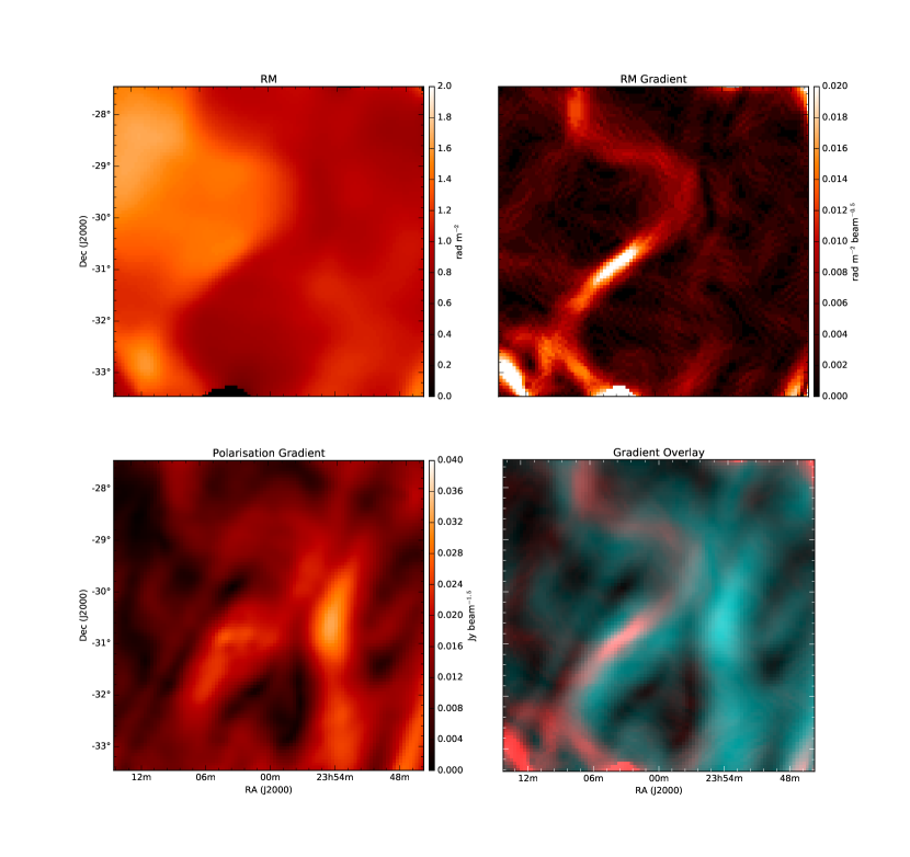
Figure 19: A zoomed in view of a region containing both significant polarized flux and smooth RM variations. [Top Left] Map showing RM (rad m^-2) at peak polarized intensity for each pixel in the Faraday depth cube. The map is the same as that highlighted by the dashed square in Figure 6 but with a colour scale that highlights finer variations in RM. [Top Right] The rotation measure gradient map (rad m^-2 beam^-0.5) - $\lvert\nabla\phi\rvert$. This is the spatial gradient of the RM map (shown top left). [Bottom Left] The polarization gradient map (Jy beam^-1.5) - $\lvert\mathbf{\nabla P}\rvert$. The map is the same as that highlighted by the dashed square in Figure 12 for the time-averaged and band-averaged epoch 1 data but with a different colour scale. [Bottom Right] Overlap map of RM gradient (red) and polarization gradient (cyan).

4.6 Structure function

In Section 4.5 we investigated possible causes for the structures seen in the polarization gradient maps and concluded that they could result from a combination of both instrinsically polarized structures and a foreground Faraday screen. An alternate method of distinguishing between these two causes is through a structure function analysis (Sun et al., 2014). The structure function of complex polarization ($P=Q+iU$) and that of polarized intensity ($p=\lvert P\rvert$) are defined respectively as:

$$SF_{P}\left(\delta\theta\right)\equiv\left<\left\lvert P\left(\theta\right)-P\left(\theta+\delta\theta\right)\right\rvert^{2}\right>$$ (11)

$$SF_{p}\left(\delta\theta\right)\equiv\left<\left[p\left(\theta\right)-p\left(\theta+\delta\theta\right)\right]^{2}\right>$$ (12)

Here $\delta\theta$ is the angular separation between two lines of sight. A comparison of the two structure functions can indicate whether the observed polarized structures are intrinsic or caused by Faraday screens (Sun et al., 2014). For intrinsic polarization there will be no correlation between polarized intensity and polarization angle, so the slope of $SF_{p}$ will be similar to that of $SF_{P}$. Alternatively, if the polarized structures are caused by Faraday screens with beam depolarization, then the slope of $SF_{P}$ will be flatter than $SF_{p}$ since much of the intrinsic structure will be smeared out by Faraday screens.

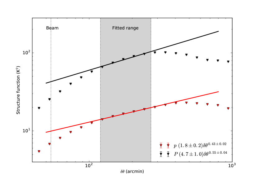
Figure 20: Structure function for epoch 1 data in the EoR-0 field using ionosphere-corrected continuum images. The fit to the curve in the region marked in grey ($120\arcmin<\delta\theta<270\arcmin$) is shown for both $p$ and $P$. The beam is marked by a dotted line at $54\arcmin$. The noise floor is not shown here but it is $\sim$$4$ orders of magnitude below each of the fitted curves.

The resulting structure functions for $SF_{p}$ and $SF_{P}$ are shown in Figure 20 for epoch 1 observations of the EoR-0 field. At angular separations less than about $90\arcmin$, the slope of the structure function effectively represents the smoothing effect of the MWA PSF ($54\arcmin$). At very large angular separations, the structure function is less constrained because of limited sensitivity of the MWA to structures $\gtrsim 10\arcdeg$ and the available field-of-view ($25\arcdeg\times 25\arcdeg$). For this analysis, we focus on the region between $120\arcmin<\delta\theta<270\arcmin$ to avoid data affected by instrumental constraints. If the slope of $SF_{P}$ were flatter than that of $SF_{p}$ this would be suggestive of polarization caused by Faraday screens (Sun et al., 2014).

In observations of the Galactic plane at 4.8 GHz, Sun et al. (2014) also find evidence of intrinsic polarization whereas at 2.3 GHz a structure function analysis suggests the presence of a Faraday screen. The reasoning for the different behaviour is that higher frequency observations (4.8 GHz) probe more deeply as they are less affected by the presence of a Faraday screen. One would expect that MWA observations would be particularly sensitive to the effects of a Faraday screen because they are observed at long wavelengths. However, the structure function analysis suggests that the observed diffuse polarization is intrinsic in nature and must therefore be associated with structures that are very local.

This is consistent with the multi-frequency polarization gradient analysis performed in Section 4.5, which found evidence of both intrinsic and Faraday screen causes for the observed polarization gradients. Currently, the structure function analysis is limited by the effective range of angular separations that could be used. Deconvolution and imaging of even larger fields would aid in widening this range and improving the structure function analysis; however, this will be left for future work.

4.7 Faraday Depth Structure

As described in Section 3.3, the 154 MHz MWA observations provide a narrow RMSF of $\delta\phi=2.3$ rad m^-2. Combined with the maximum-scale size sensitivity of 1.0 rad m^-2 the MWA observations are only able to detect simple components even in the presence of Faraday complex structure. A Faraday-thin structure, however, would result in a simple FDF with a single component; see Appendix B of Brentjens & de Bruyn (2005).

A mix of structures has been observed in Faraday spectra observed in the Galactic anti-center with the Westerbork Synthesis Radio Telescope (WSRT) at 324-387 MHz with $\sim$$3\arcmin$ resolution (Schnitzeler et al., 2007, 2009). The vast majority of lines of sight observed in a $9\arcdeg\times 9\arcdeg$ field have Faraday spectra that are reasonably well fit by a simple model dominated by a single bright peak. Only a small fraction of lines of sight exhibit Faraday complexity.

Looking at the Faraday spectra from the 154 MHz MWA EoR-0 observations, the vast majority of Faraday structure is simple and dominated by peaks at low RM; see Figures 7 and 8. The Faraday spectra are similar to those observed in diffuse polarization at similar wavelengths with LOFAR in the ELAIS-N1 (Jelić et al., 2014) and 3C196 fields (Jelić et al., 2015) . It is unlikely that these are unresolved Faraday-thick structures because of the excellent resolution available in Faraday space with the MWA. Without introducing a more involved scenario, in which a secondary peak in Faraday space is weakened to a level below our detection threshold, a simple explanation of the peak is that . This would be consistent with findings of the polarization gradient function analysis and the structure function analysis discussed in Sections 4.5 and 4.6.

5 Conclusions

We have presented a 625 square degree survey of diffuse linear polarization at 154 MHz carried out with the MWA. The survey, centered on the MWA EoR-0 field (0^h, -27°), achieved a sensitivity of 5.9 mJy beam^-1 at $\sim$$54\arcmin$ resolution. The compact baselines of the MWA have been shown to be particularly sensitive to diffuse structures spanning $1\arcdeg-10\arcdeg$, something that has traditionally only been within reach of single-dish instruments.

Our MWA observations reveal smooth large-scale diffuse structures that are $\sim$$1\arcdeg-8\arcdeg$ in extent in linear polarization and clearly detected even in 2 minute snapshots. The brightness temperature of these structures is on average 4 K in polarized intensity, peaking at 11 K. We estimate a distance of $51\pm 20$ pc to the polarized emission based on RM measurements of the in-field pulsar PSR J2330$-$2005.

Rotation measure synthesis reveals that the structures have Faraday depths ranging from $-2$ rad m^-2 to 10 rad m^-2. A large fraction of these peak at $+1.0$ rad m^-2 but smaller structures are also observed to peak at $+3.0$, $+7.1$ and $\sim$$+9$ rad m^-2. The observed RM structure is smooth, particularly around the region where polarized intensity peaks, with a peak RM gradient of $\sim$$0.02$ rad m^-2 beam^-0.5.

The sensitivity available in our deep observations allowed a frequency-dependent analysis of the polarized structure to be performed for the first time at long wavelengths. The results of the analysis suggested that the polarized structures are dominated by intrinsic emission but may also have a component that is due to a foreground Faraday screen. A structure function analysis of our linearly polarized images and an analysis of Faraday structure also suggest that intrinsic polarized emission tends to dominate.

A 400 square degree subset of the field was re-imaged at full resolution ($\sim$$2.4\arcmin$) and 2.3 mJy beam^-1 sensitivity to search for polarized point sources. We detect 4 extragalactic linearly polarized point sources within the EoR-0 field and have confirmed these by observing the shift in their RM over two epochs as a result of observably different ionospheric conditions in those epochs. Based on known polarized field sources at 1.4 GHz and non-detections at 154 MHz, we estimate an upper limit on the depolarization ratio of 0.08 from 1.4 GHz to 154 MHz. Such levels of depolarization are not surprising at long wavelengths, however, we note that the four detected sources did not exhibit significantly increased levels of depolarization compared to 1.4 GHz. This may hint towards a small population of sources (one per 100 sq. deg) with this behaviour. We also note that these may be associated with relatively large radio galaxies where unresolved polarized hot spots lie outside of the local environment and are less likely to suffer the effects of depolarization.

With its high sensitivity to large-scale structure, the MWA has proven itself to be a formidable instrument for the study of diffuse polarization in the local ISM. In combination with RM synthesis, it also provides a unique ability to measure the effect of ionospheric Faraday rotation on the diffuse polarized background both spatially ($\sim$$1\arcdeg$ resolution) and temporally ($\sim$$2$ minute resolution). This not only allows ionospheric effects to be calibrated without the need for ionospheric models but also provides an opportunity to observe local solar events by measuring their effect on the background RM.

The survey presented in this paper utilized only a very small fraction of the data currently available in the EoR and GLEAM projects. There is great potential to extend the survey to look more deeply within the EoR fields, to look over an increased field-of-view with the GLEAM data, and also to explore the full $80$–$230$ MHz range of frequencies available in the GLEAM data. Additional epochs of GLEAM data will aid in improving sensitivity and mitigating the sidelobe confusion that affects some snapshots. An implementation of an improved beam model will drastically reduce the apparent leakage observed in the highest frequency bands and so increase the range of reliable data available for subsequent frequency-dependent analysis. Furthermore, deconvolution of the diffuse structure and a multi-scale analysis of the gradient of linear polarization, e.g. Robitaille & Scaife (2015), would allow the observations to probe more deeply.

While the sensitivity of the observations presented in this paper prevented such an analysis, a measurement of instrumental leakage from linear polarization into total intensity would provide valuable information to the EoR community. Understanding leakage of this form is of particular importance for EoR science because it can act as a possible contamination source for EoR measurements (Jelić et al., 2008; Geil et al., 2011; Moore et al., 2013; Asad et al., 2015). This has been left for future work and will be performed once the new MWA beam model has been implemented. An improved analysis will also be possible with an extension to the MWA that is currently underway. The extension provides additional compact configurations and redundant baselines that will aid in calibration.

References

- Arora et al. (2015) Arora, B. S., Morgan, J., Ord, S. M., et al. 2015, PASA, 32, e029
- Asad et al. (2015) Asad, K. M. B., Koopmans, L. V. E., Jelić, V., et al. 2015, MNRAS, 451, 3709
- Baars et al. (1977) Baars, J. W. M., Genzel, R., Pauliny-Toth, I. I. K., & Witzel, A. 1977, A&A, 61, 99
- Beck et al. (1996) Beck, R., Brandenburg, A., Moss, D., et al. 1996, ARA&A, 34, 155
- Beck (2007) Beck, R. 2007, A&A, 470, 539
- Berdyugin & Teerikorpi (2001) Berdyugin, A., & Teerikorpi, P. 2001, A&A, 368, 635
- Berdyugin et al. (2004) Berdyugin, A., Piirola, V., & Teerikorpi, P. 2004, A&A, 424, 873
- Berdyugin et al. (2014) Berdyugin, A., Piirola, V., & Teerikorpi, P. 2014, A&A, 561, A24
- Berkhuijsen et al. (2006) Berkhuijsen, E. M., Mitra, D., & Mueller, P. 2006, Astronomische Nachrichten, 327, 82
- Bernardi et al. (2009) Bernardi, G., de Bruyn, A. G., Brentjens, M. A., et al. 2009, A&A, 500, 965
- Bernardi et al. (2010) Bernardi, G., de Bruyn, A. G., Harker, G., et al. 2010, A&A, 522, A67
- Bernardi et al. (2013) Bernardi, G., Greenhill, L. J.; Mitchell, D. A. et al. 2013, ApJ, 771, 105
- Bowman et al. (2013) Bowman, J. D., Cairns, I., Kaplan, D. L., et al. 2013, PASA, 30, 31
- Brentjens & de Bruyn (2005) Brentjens, M. A., & de Bruyn, A. G. 2005, A&A, 441, 1217
- Burkhart et al. (2012) Burkhart, B., Lazarian, A., & Gaensler, B. M. 2012, ApJ, 749, 145
- Burn (1966) Burn, B. J. 1966, MNRAS, 133, 67
- Calabretta et al. (2014) Calabretta, M. R., Staveley-Smith, L., & Barnes, D. G. 2014, PASA, 31, e007
- Carretti (2010) Carretti, E. 2010, in ASP Conf. Ser. 438, The Dynamic Interstellar Medium: A Celebration of the Canadian Galactic Plane Survey, ed. R. Kothes, T. L. Landecker, & A. G. Willis (San Francisco, CA: ASP), 276
- Cendes & AARTFAAC Project Team (2012) Cendes, Y., & AARTFAAC Project Team 2012, American Astronomical Society Meeting Abstracts #219, 219, 422.36
- Ellingson et al. (2009) Ellingson, S. W., Clarke, T. E., Cohen, A., et al. 2009, IEEE Proceedings, 97, 1421
- Fletcher & Shukurov (2007) Fletcher, A., & Shukurov, A. 2007, EAS Publications Series, 23, 109
- Franzen et al. (2015) Franzen, T. M. O., Jackson, C. A., Callingham, J. R., et al. 2015, The many facets of extragalactic radio surveys: towards new scientific challenges (EXTRA-RADSUR2015). 20-23 October 2015, Bologna, Italy. http://pos.sissa.it/archive/conferences/267/003/EXTRA-RADSUR2015_053.pdf
- Gaensler et al. (2011) Gaensler, B. M., Haverkorn, M., Burkhart, B., et al. 2011, Nature, 478, 214
- Gaensler et al. (2001) Gaensler, B. M., Dickey, J. M., McClure-Griffiths, N. M., et al. 2001, ApJ, 549, 959
- Gaensler et al. (2008) Gaensler, B. M., Madsen, G. J., Chatterjee, S., & Mao, S. A. 2008, PASA, 25, 184
- Geil et al. (2011) Geil, P. M., Gaensler, B. M., & Wyithe, J. S. B. 2011, MNRAS, 418, 516
- Gray et al. (1998) Gray, A. D., Landecker, T. L., Dewdney, P. E., & Taylor, A. R. 1998, Nature, 393, 660
- Guzmán et al. (2011) Guzmán, A. E., May, J., Alvarez, H., & Maeda, K. 2011, A&A, 525, A138
- Hamilton & Lyne (1987) Hamilton, P. A., & Lyne, A. G. 1987, MNRAS, 224, 1073
- Han et al. (2013) Han, J. L., Reich, W., Sun, X. H., et al. 2013, International Journal of Modern Physics Conference Series, 23, 82
- Haslam et al. (1982) Haslam, C. G. T., Salter, C. J., Stoffel, H., & Wilson, W. E. 1982, A&AS, 47, 1
- Haverkorn et al. (2000) Haverkorn, M., Katgert, P., & de Bruyn, A. G. 2000, A&A, 356, L13
- Haverkorn et al. (2003a) Haverkorn, M., Katgert, P., & de Bruyn, A. G. 2003a, A&A, 403, 1031
- Haverkorn et al. (2003b) Haverkorn, M., Katgert, P., & de Bruyn, A. G. 2003b, A&A, 403, 1045
- Haverkorn et al. (2003c) Haverkorn, M., Katgert, P., & de Bruyn, A. G. 2003c, A&A, 404, 233
- Haverkorn & Heitsch (2004) Haverkorn, M., & Heitsch, F. 2004, A&A, 421, 1011
- Haverkorn et al. (2015) Haverkorn, M., Akahori, T., Carretti, E., et al. 2015, Proceedings of Science, Advancing Astrophysics with the Square Kilometre Array (AASKA14), 96
- Heald (2009) Heald, G. 2009, IAU Symposium, 259, 591
- Hurley-Walker et al. (2014) Hurley-Walker, N., Morgan, J., Wayth, R. B., et al. 2014, PASA, 31, e045
- Iacobelli et al. (2013) Iacobelli, M., Haverkorn, M., & Katgert, P. 2013, A&A, 549, A56
- Iacobelli et al. (2014) Iacobelli, M., Burkhart, B., Haverkorn, M., et al. 2014, A&A, 566, A5
- Ishwara-Chandra & Saikia (1999) Ishwara-Chandra, C. H., & Saikia, D. J. 1999, MNRAS, 309, 100
- Jacobs et al. (2016) Jacobs, D. C., Hazelton, B. J., Trott, C. M., et al. 2016, ApJ, accepted (arXiv:1605.06978)
- Jelić et al. (2008) Jelić, V., Zaroubi, S., Labropoulos, P., et al. 2008, MNRAS, 389, 1319
- Jelić et al. (2014) Jelić, V., de Bruyn, A. G., Mevius, M., et al. 2014, A&A, 568, 101
- Jelić et al. (2015) Jelić, V., de Bruyn, A. G., Pandey, V. N., et al. 2015, A&A, 583, 137
- Johnston et al. (2007) Johnston, S., Kramer, M., Karastergiou, A., et al. 2007, MNRAS, 381, 1625
- Kaplan et al. (2015) Kaplan, D. L., Tingay, S. J., Manoharan, P. K., et al. 2015, ApJ, 809, L12
- Lallement et al. (2003) Lallement, R., Welsh, B. Y., Vergely, J. L., et al. 2003, A&A, 411, 447
- Landecker et al. (2002) Landecker, T. L., Uyanıker, B., & Kothes, R. 2002, in Astrophysical Polarized Backgrounds, ed. S. Cecchini, S. Cortiglioni, R. Sault, & C. Sbarra, Vol. 609 (Melville, NY: American Institute of Physics), 9-14
- Li et al. (2011) Li, F., Brown, S., Cornwell, T. J., & de Hoog, F. 2011, A&A, 531, A126
- Loi et al. (2015a) Loi, S. T., Murphy, T., Cairns, I. H., et al. 2015a, Geophys. Res. Lett., 42, 3707
- Loi et al. (2015b) Loi, S. T., Trott, C. M., Murphy, T., et al. 2015b, Radio Science, 50, 574
- Loi et al. (2015c) Loi, S. T., Murphy, T., Bell, M. E., et al. 2015c, MNRAS, 453, 2731
- Manchester et al. (2005) Manchester, R. N., Hobbs, G. B., Teoh, A., & Hobbs, M. 2005, AJ, 129, 1993
- Mao et al. (2010) Mao, S. A., Gaensler, B. M., Haverkorn, M., et al. 2010, ApJ, 717, 1170
- Mathewson & Milne (1965) Mathewson, D. S. & Milne, M. F. 1965, AuJPh, 18, 635
- McCulloch et al. (1978) McCulloch, P. M., Hamilton, P. A., Manchester, R. N., & Ables, J. G. 1978, MNRAS, 183, 645
- McKee & Ostriker (2007) McKee, C. F., & Ostriker, E. C. 2007, ARA&A, 45, 565
- Mitchell et al. (2008) Mitchell, D. A., Greenhill, L. J., Wayth, R. B., et al. 2008, IEEE Journal of Selected Topics in Signal Processing, 2, 707
- Moore et al. (2013) Moore, D. F., Aguirre, J. E., Parsons, A. R., et al. 2013, ApJ, 769, 154
- Moore et al. (2016) Moore, D., Aguirre, J. E., Parsons, A., et al. 2016, ApJ, submitted (arXiv:1502.05072)
- Mulcahy et al. (2014) Mulcahy, D. D., Horneffer, A., Beck, R., et al. 2014, A&A, 568, A74
- Nord et al. (2006) Nord, M. E., Henning, P. A., Rand, R. J., et al. 2006, AJ, 132, 242
- Oberoi & Kasper (2004) Oberoi, D., & Kasper, J. C. 2004, Planet. Space Sci., 52, 1415
- Offringa et al. (2012) Offringa, A. R., van de Gronde, J. J., & Roerdink, J. B. T. M. 2012, A&A, 539, A95
- Offringa et al. (2014) Offringa, A. R., McKinley, B., Hurley-Walker, N., et al. 2014, MNRAS, 444, 606
- Offringa et al. (2015) Offringa, A. R., Wayth, R. B., Hurley-Walker, N., et al. 2015, PASA, 32, e008
- Offringa et al. (2016) Offringa, A. R., Trott, C. M., Hurley-Walker, N., et al. 2016, MNRAS, 458, 1057
- Oppermann et al. (2015) Oppermann, N., Junklewitz, H., Greiner, M., et al. 2015, A&A, 575, A118
- Ord et al. (2010) Ord, S. M., Mitchell, D. A., Wayth, R. B., et al. 2010, PASP, 122, 1353
- Ord et al. (2015) Ord, S. M., Crosse, B., Emrich, D., et al. 2015, PASA, 32, e006
- Paul et al. (2014) Paul, S., Sethi, S. K., Subrahmanyan, R., et al. 2014, ApJ, 793, 28
- Peterson & Webber (2002) Peterson, J. D., & Webber, W. R. 2002, ApJ, 575, 217
- Puspitarini et al. (2014) Puspitarini, L., Lallement, R., Vergely, J.-L., & Snowden, S. L. 2014, A&A, 566, A13
- Reid et al. (1999) Reid, R. I., Kronberg, P. P., & Perley, R. A. 1999, ApJS, 124, 285
- Remazeilles et al. (2015) Remazeilles, M., Dickinson, C., Banday, A. J., et al. 2015, MNRAS, 451, 4311
- Robitaille & Scaife (2015) Robitaille, J.-F., & Scaife, A. M. M. 2015, MNRAS, 451, 372
- Sault et al. (1995) Sault, R. J., Teuben, P. J., & Wright, M. C. H. 1995, in R. A. Shaw, H. E. Payne, & J. J. E. Hayes ed., Astronomical Data Analysis Software and Systems IV Vol. 77 of ASP Conference Series. p. 433
- Sault et al. (1996) Sault, R. J., Hamaker, J. P., & Bregman, J. D. 1996, A&AS, 117, 149
- Schnitzeler et al. (2007) Schnitzeler, D. H. F. M., Katgert, P., & de Bruyn, A. G. 2007, A&A, 471, L21
- Schnitzeler et al. (2009) Schnitzeler, D. H. F. M., Katgert, P., & de Bruyn, A. G. 2009, A&A, 494, 611
- Shukurov & Berkhuijsen (2003) Shukurov, A., & Berkhuijsen, E. M. 2003, MNRAS, 342, 496
- Slee (1977) Slee, O. B. 1977, Australian Journal of Physics Astrophysical Supplement, 43, 1
- Slee (1995) Slee, O. B. 1995, Australian Journal of Physics, 48, 143
- Sokoloff et al. (1998) Sokoloff, D. D., Bykov, A. A., Shukurov, A., et al. 1998, MNRAS, 299, 189
- Sotomayor-Beltran et al. (2013) Sotomayor-Beltran, C., Sobey, C., Hessels, J. W. T., et al. 2013, A&A, 552, A58
- Stovall et al. (2015) Stovall, K., Ray, P. S., Blythe, J., et al. 2015, ApJ, 808, 156
- Sutinjo et al. (2015) Sutinjo, A., O’Sullivan, J., Lenc, E., et al. 2015, Radio Science, 50, 52
- Sun et al. (2008) Sun, X. H., Reich, W., Waelkens, A., & Enßlin, T. A. 2008, A&A, 477, 573
- Sun et al. (2011) Sun, X. H., Reich, W., Han, J. L., et al. 2011, A&A, 527, A74
- Sun et al. (2014) Sun, X. H., Gaensler, B. M., Carretti, E., et al. 2014, MNRAS, 437, 2936
- Taylor & Cordes (1993) Taylor, J. H., & Cordes, J. M. 1993, ApJ, 411, 674
- Taylor et al. (2003) Taylor, A. R., Gibson, S. J., Peracaula, M., et al. 2003, AJ, 125, 3145
- Taylor et al. (2009) Taylor, A. R., Stil, J. M., & Sunstrum, C. 2009, ApJ, 702, 1230
- Thyagarajan et al. (2015) Thyagarajan, N., Jacobs, D. C., Bowman, J. D., et al. 2015, ApJ, 804, 14
- Tingay et al. (2013) Tingay, S. J., Goeke, R., Bowman, J. D., et al. 2013, PASA, 30, 7
- Trott (2014) Trott, C. M. 2014, PASA, 31, e026
- Uyanıker et al. (2003) Uyanıker, B., Landecker, T. L., Gray, A. D., & Kothes, R. 2003, ApJ, 585, 785
- van Haarlem et al. (2013) van Haarlem, M. P., Wise, M. W., Gunst, A. W., et al. 2013, A&A, 556, A2
- Vinyaikin & Paseka (2015) Vinyaikin, E. N., & Paseka, A. M. 2015, Astronomy Reports, 59, 672
- Wayth et al. (2015) Wayth, R. B., Lenc, E., Bell, M. E., et al. 2015, PASA, 32, e025
- Wieringa et al. (1993) Wieringa, M. H., de Bruyn, A. G., Jansen, D., et al. 1993, A&A, 268, 215
- Willis et al. (2016) Willis, A. G., Mevius, M., Anderson, J. M., et al. 2016, Astronomy and Computing, submitted
- Wolleben et al. (2006) Wolleben, M., Landecker, T. L., Reich, W., & Wielebinski, R. 2006, A&A, 448, 411
- Wolleben (2007) Wolleben, M. 2007, ApJ, 664, 349
- Wright (2006) Wright, E. L. 2006, PASP, 118, 1711
- Wrobel & Walker (1999) Wrobel, J. M., & Walker, R. C. 1999, Synthesis Imaging in Radio Astronomy II, 180, 171