Theory for the Acoustic Raman Modes of Proteins

Abstract

We present a theoretical analysis that associates the resonances of extraordinary acoustic Raman (EAR) spectroscopy [Wheaton et al., Nat Photon 9, 68 (2015)] with the collective modes of proteins. The theory uses the anisotropic elastic network model to find the protein acoustic modes, and calculates Raman intensity by treating the protein as a polarizable ellipsoid. Reasonable agreement is found between EAR spectra and our theory. Protein acoustic modes have been extensively studied theoretically to assess the role they play in protein function; this result suggests EAR as a new experimental tool for studies of protein acoustic modes.

The central dogma of molecular biology involves one-way information transfer from DNA to protein, a process that directly and reliably associates a particular three-dimensional structure with a given amino acid sequence. Each structure is associated with a function (or functions); often, for example, a particular structure catalyzes a chemical reaction with remarkable selectivity. The vibrational modes of a protein reflect its structure and conformation, and are thought to facilitate allostery and conformational change Chou (1988); Nicolaï et al. (2014); Yang et al. (2007); Dobbins et al. (2008); Zheng and Thirumalai (2009); Tama and Sanejouand (2001). Of these modes, those with the lowest frequency are termed acoustic modes, and represent the largest thermal fluctuations of the protein.

Whereas many spectroscopic methods can probe localized resonances in a protein Cavanagh et al. (2007); Skoog et al. (2007), delocalized collective modes and their role in biological function have been historically difficult to measure Turton et al. (2014). In the gigahertz (GHz) to low terahertz (THz) spectral window, electromagnetic absorption experiments have to deal with high solvent absorption and dielectric mixtures Markelz et al. (2002); Xu et al. (2006); Vinh et al. (2011). Other experimental techniques for studying acoustic protein modes include inelastic incoherent neutron scattering (IINS) Middendorf (1984) and optical Kerr-effect (OKE) spectroscopy Turton et al. (2014).

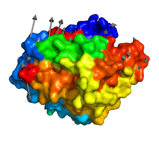
(a)     ANM eigenmode.

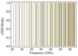
(b)     Frequency spectrum, plotted with unit amplitudes.

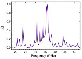
(c)     Raman intensity spectrum (same protein modes as (b)).

Figure 1: The method by which our protein Raman spectra are computed (shown here for carbonic anhydrase). ANM yields a set of eigenvalues and eigenvectors; a sample eigenvector is shown in (a). The set of eigenvalues (related to the frequencies) is shown in (b). The eigenmodes are applied to generate positive and negative displacements for each mode, and the resulting protein shapes are fit to ellipsoids. Analytic expressions are used to compute a Raman intensity for each mode. The spectrum shown in (c) centers a Lorentzian function, multiplied by its Raman intensity (RI), at the position of each mode shown in (b). As seen, a small subset of the original ANM modes are dominant in the Raman spectrum.

We recently reported extraordinary acoustic Raman (EAR) spectroscopy as a way to measure resonances of optically trapped nanoparticles Wheaton et al. (2015). In EAR, the $\sim$10 to 100 GHz beating of two trapping lasers creates increased RMS fluctuation when the beat frequency matches a Raman-active particle resonance. The frequency of vibrational modes in single polystyrene nanospheres were shown to fit with Lamb’s theory. The EAR spectra of several proteins were measured, however the remaining challenge is “…to associate the observed [protein] resonances with specific motions…” Weigel and Kukura (2015). Here we propose a theory that assigns the measured EAR modes to low-frequency Raman-active protein modes.

Our theory uses elastic network model (ENM) normal mode analysis; elastic network models reproduce the essential dynamics of low-frequency protein modes to good accuracy Tirion (1996). We use the ENM known as the anisotropic network model (ANM) Doruker et al. (2000); Atilgan et al. (2001), as implemented in ProDy Bakan et al. (2011).

ANM represents the potential surface of an $N$ atom protein (excluding hydrogen) using a network of springs with spring constant $k$. ANM analyses are often done using a reduced set of atoms, namely the $C_{\alpha}$ atoms along the protein backbone; we use an all-atom approach (excluding hydrogen) to build the elastic network. Each spring connects a pair of atomic coordinates, but only atoms within cutoff radius $r_{c}$ are connected. The matrix of second derivatives (taken with respect to the Cartesian coordinates of each atom) of this potential, known as the Hessian, is then computed; it is an $N\times N$ matrix of $3\times 3$ (the protein coordinates are in $\mathbb{R}^{3}$) super-elements and has the units of $k$. The diagonalization of this matrix yields $3N-6$ non-zero eigenvalues $\lambda_{i}$ and eigenvectors $Q_{i}$ that correspond to the frequency $\omega_{i}=\sqrt{\lambda_{i}/m}$ and the displacement from equilibrium of each mode $i$. $m$ is the mass of an atom; we use 13.2 amu for all atoms (a weighted average). The six zero-valued eigenvalues correspond to rotational and translational degrees of freedom. Fig. 1(a) shows what one of these eigenvectors $Q_{i}$ looks like for a protein. At this point, we have a set of mode frequencies, as shown in Fig. 1(b).

To calculate the intensity of each mode, we need to compute the Raman intensity of a given ANM mode from positive and negative coordinate displacements $\vec{r}_{i,\pm}=\vec{r}_{0}\pm\beta\vec{Q}_{i}$. The equilibrium coordinates are $\vec{r}_{0}$; $\vec{Q}_{i}$ is a unit vector in $\mathbb{R}^{3N}$ and $\beta$ is a small scaling parameter. We construct a quantity closely related to the inertia tensor, and diagonalize it to find the semi-principle axes (unit vectors) and lengths $a_{i,\pm},b_{i,\pm},c_{i,\pm}$ of two best-fitting ellipsoids Jang-Condell and Hernquist (2001), one for each of the stretched protein coordinates. Dielectric polarizability tensors $\alpha_{i,\pm}$ for these best-fitting ellipsoids are then computed, using analytic expressions Sihvola (1999); Stoner (1945) that require only the semi-principle axis lengths and the internal and external relative dielectric permittivity. We take the two permittivity values to be $\epsilon_{i}=n^{2}=1.6^{2}$ (protein) McMeekin et al. (1962) and $\epsilon_{e}=1.33^{2}$ (water).

Name	Molecular Weight (kDa)	PDB ID	ANM Spring Constant k (kJ mol${}^{-}1$ Å-2)
pancreatic trypsin inhibitor	6.6	5PTI Wlodawer et al. (1984)	1.51
carbonic anhydrase I	29.7	1CRM Kannan et al. (1984)	1.28
streptavidin	52.8	3RY2 Le Trong et al. (2011)	1.29
ovotransferrin	76.2	1OVT Kurokawa et al. (1995)	0.79
cyclooxygenase-2	274.4	5COX Kurumbail et al. (1996)	1.15

Table 1: Summary of proteins measured experimentally and the associated PDB structure files (coordinate data) used here.

The Raman polarizability $\alpha^{\prime}_{i}=(\partial\alpha_{i}/\partial Q_{i})_{0}$ measures the change in polarizability due to the difference between the protein coordinates $\vec{r}_{i,\pm}$ Woodward (1967). We calculate this as $\alpha^{\prime}_{i}\sim\alpha_{i,+}-\alpha_{i,-}$. We also account for the possibility that the two best-fit ellipsoids have rotated under the action of the pair of mode displacements by rotating one of the polarizability tensors as a rank two tensor, using the rotation matrix formed using the pair of best-fit semi-principle axes Hand and Finch (1998). With this, the Raman intensity $I_{i}$ of ANM mode $i$ is given by Woodward (1967)

$$I_{i}\sim 45\bar{\alpha}^{\prime 2}_{i}+4\gamma^{\prime 2}_{i}$$ (1)

where

$$\bar{\alpha}_{i}^{\prime} =\frac{1}{3}(\alpha^{\prime}_{i,xx}+\alpha^{\prime}_{i,yy}+\alpha^{\prime}_{i,zz})$$ (2)

$$\gamma^{\prime 2}_{i} =\frac{1}{2}((\alpha^{\prime}_{i,xx}-\alpha^{\prime}_{i,yy})^{2}+(\alpha^{\prime}_{i,yy}-\alpha^{\prime}_{i,zz})^{2}$$

$$+(\alpha^{\prime}_{i,zz}-\alpha^{\prime}_{i,xx})^{2}+6(\alpha^{\prime 2}_{i,xy}+\alpha^{\prime 2}_{i,yz}+\alpha^{\prime 2}_{i,zx})).$$ (3)

The mean value $\bar{\alpha}^{\prime}_{i}$ measures change in polarizability of a particular mode due to linear stretching; $\gamma^{\prime}_{i}$ gives the anisotropic contribution. Spectra (see for example Fig. 1(c)) are constructed by centering Lorentzian functions at the frequency position $\omega_{i}$ of each mode, with mode heights proportional to the Raman intensities $I_{i}$ (and plotting the summation of these curves). We choose a constant Lorentzian linewidth for each spectrum.

We compare our theory with previously published experimental data Wheaton et al. (2015) for the five proteins listed in Table 1, and list the Research Collaboratory for Structural Bioinformatics Protein Data Bank (RCSB PDB) Berman et al. (2007) structures used in computation. (The streptavidin data was not published but was acquired during the same period.) It is assumed that the PDB crystal coordinates are close to the potential minimum (i.e. that the crystal coordinates approximately give $\vec{r}_{0}$). By matching the atomic mean-square fluctuations predicted by ANM (calculated using ProDy) with the crystallographic isotropic temperature factors included with the PDB crystal data, we associate a $k$ with each protein Atilgan et al. (2001). These $k$ values are shown in Table 1. Details of these ANM, spring constant, ellipsoid fitting and Raman calculations are given in the supporting information.

EXPERIMENT                                                  THEORY

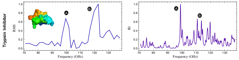
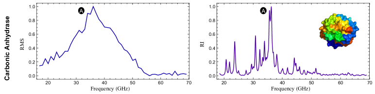
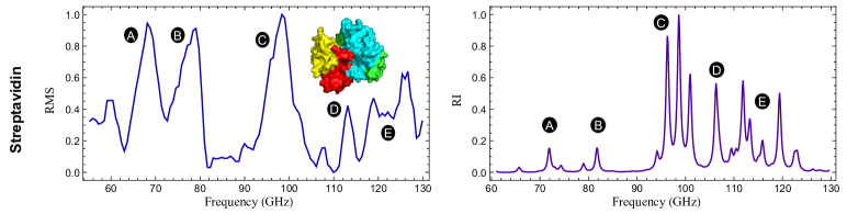
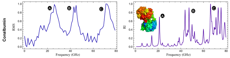
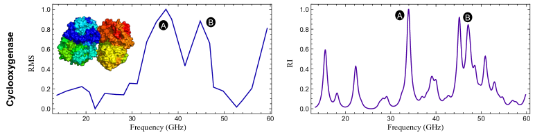
Figure 2: A comparison of the experimentally measured extraordinary acoustic Raman (EAR) spectra (left) and elastic network/Raman ellipsoid polarizability model spectra (right). RMS is the root-mean-squared variation in the optical trap transmission. RI is the theoretical Raman intensity, calculated using an all-atom ANM with cutoff radius of $r_{c}$=7.9 Å. Suggested correlations between theory and experiment of selected peaks (or groups of peaks) are letter-labelled.

The ANM cutoff distance $r_{c}=7.9$ Å was selected by hand for best overall agreement between theory and experiment for the five proteins. At values near this $r_{c}$, EAR mode frequencies $\tilde{\omega}_{i}$ and ANM frequencies $\omega_{i}$ are approximately linearly proportional: $\tilde{\omega}_{i}=\zeta\omega_{i}$. The proportionality constant $\zeta$ is a free parameter in our theory; a $\zeta$ is chosen for each protein (see supporting information). It is the fine spectral resolution of EAR that allows us to directly fit the spectral modes for each protein; in prior works obtaining a Gaussian-distributed density of states has been used as a criterion for selecting physical values for $r_{c}$ Atilgan et al. (2001).

The computed spectra along with our previously obtained experimental EAR spectra are shown in Fig. 2. The visual agreement between theory (right side) and experiment (on the left) in Fig. 2 is, in our opinion, quite remarkable. The intensity and frequency placement of the major peaks, as well as some of the minor peaks, agree with the experimental data. We have made many approximations, including the use of a “spring network” potential in place of a more realistic potential map (e.g. the semiempirical potentials employed in molecular dynamics) and the representation of protein polarizability by the polarizability of a dielectric ellipsoid. The normal modes could also be computed in the time domain, by combining molecular dynamics simulation with principal component analysis to accurately capture the low-frequency modes Bahar et al. (2010). Wider bandwidth Raman intensity spectra for each protein are given in the supporting information. As can be seen in the extended spectra, the EAR data shown here have captured most of the major Raman-active collective modes in these five proteins.

In the light of our theory, we make some comments regarding the experiment. A past optical trapping work by our group Pang and Gordon (2012) reported on a special type of conformational change, the N-F transition, found in bovine serum albumin (BSA); this conformation change can be viewed as a type of denaturation as it involves a reversible unfolding of BSA domain III Rosenoer et al. (2014); Khan (1986). BSA can also be irreversibly denatured Wetzel et al. (1980). We assume here, as we did in the EAR experiment Wheaton et al. (2015), that the trapped proteins have not been irreversibly denatured. We also assume that the proteins are not being reversibly unfolded or deformed by the optical forces, so that the equilibrium coordinates given by the x-ray crystal data will be good approximations of the optically trapped protein coordinates. Past works (e.g. Brooks and Karplus (1983); Go et al. (1983)) have suggested that anharmonic effects play a role in the low frequency modes of proteins, whereas our ANM-based theory is a purely harmonic model of protein motion. In a Duffing oscillator, for example, the absence of nonlinear effects such as jumping, hysteresis, and bistability can be related to the fact that harmonic driving force is sufficiently weak (Enns and McGuire, 2012, Chapter 7). Thus an explanation for the seeming unimportance of anharmonicity in our theory is that the amplitude of the driving force is low enough that the protein response is linear.

There has hitherto been relatively little experimental evidence for the existence of protein collective modes—accomplishments in protein THz spectroscopy have not been able to conclusively connect measurements with biologically relevant collective protein motions Turton et al. (2014). There has also been difficulty in assigning physical frequency units to ENM. These results directly connect ENM mode analysis to EAR. They provide another way to validate ENM results, and suggest EAR as a new tool for future experimental studies of low-frequency protein collective modes. They also suggest that EAR may provide a way to improve ENMs.

We would like to acknowledge the use of the computational resources of WestGrid (www.westgrid.ca) and Compute Canada (www.computecanada.ca). This work was supported in part by an NSERC Discovery Grant and funding from the Faculty of Graduate Studies at the University of Victoria. The protein renderings were prepared using PyMOL Schrödinger, LLC (2010) and POV-Ray Persistence of Vision Pty. Ltd. (2004).

References

- Chou (1988) K.-C. Chou, Biophysical Chemistry 30, 3 (1988), URL http://www.sciencedirect.com/science/article/pii/0301462288850026.
- Nicolaï et al. (2014) A. Nicolaï, P. Delarue, and P. Senet, in Computational Methods to Study the Structure and Dynamics of Biomolecules and Biomolecular Processes, edited by A. Liwo (Springer, Berlin Heidelberg, 2014).
- Yang et al. (2007) L. Yang, G. Song, and R. L. Jernigan, Biophysical Journal 93, 920 (2007), ISSN 0006-3495, URL http://www.sciencedirect.com/science/article/pii/S0006349507713498.
- Dobbins et al. (2008) S. E. Dobbins, V. I. Lesk, and M. J. E. Sternberg, Proceedings of the National Academy of Sciences 105, 10390 (2008), URL http://www.pnas.org/content/105/30/10390.abstract.
- Zheng and Thirumalai (2009) W. Zheng and D. Thirumalai, Biophysical Journal 96, 2128 (2009), URL http://www.ncbi.nlm.nih.gov/pmc/articles/PMC2717279/.
- Tama and Sanejouand (2001) F. Tama and Y.-H. Sanejouand, Protein Engineering 14, 1 (2001), URL http://peds.oxfordjournals.org/content/14/1/1.abstract.
- Cavanagh et al. (2007) J. Cavanagh, W. J. Fairbrother, A. G. P. III, M. Rance, and N. J. Skelton, Protein NMR Spectroscopy: Principles and Practice (Academic Press, Burlington; California; London, 2007), 2nd ed.
- Skoog et al. (2007) D. Skoog, F. Holler, and S. Crouch, Principles of Instrumental Analysis (Thomson Brooks/Cole, 2007).
- Turton et al. (2014) D. A. Turton, H. M. Senn, T. Harwood, A. J. Lapthorn, E. M. Ellis, and K. Wynne, Nat Commun 5 (2014), URL http://dx.doi.org/10.1038/ncomms4999.
- Markelz et al. (2002) A. Markelz, S. Whitmire, J. Hillebrecht, and R. Birge, Physics in Medicine and Biology 47, 3797 (2002), URL http://stacks.iop.org/0031-9155/47/i=21/a=318.
- Xu et al. (2006) J. Xu, K. W. Plaxco, and J. S. Allen, Protein Science 15, 1175 (2006), URL http://stacks.iop.org/0031-9155/47/i=21/a=318.
- Vinh et al. (2011) N. Q. Vinh, S. J. Allen, and K. W. Plaxco, Journal of the American Chemical Society 133, 8942 (2011), URL http://dx.doi.org/10.1021/ja200566u.
- Middendorf (1984) H. D. Middendorf, Annual Review of Biophysics and Bioengineering 13, 425 (1984), URL http://dx.doi.org/10.1146/annurev.bb.13.060184.002233.
- Wheaton et al. (2015) S. Wheaton, R. M. Gelfand, and R. Gordon, Nat Photon 9, 68 (2015), URL http://dx.doi.org/10.1038/nphoton.2014.283.
- Weigel and Kukura (2015) A. Weigel and P. Kukura, Nat Photon 9, 11 (2015), URL http://dx.doi.org/10.1038/nphoton.2014.309.
- Tirion (1996) M. M. Tirion, Phys. Rev. Lett. 77, 1905 (1996), URL http://link.aps.org/doi/10.1103/PhysRevLett.77.1905.
- Doruker et al. (2000) P. Doruker, A. R. Atilgan, and I. Bahar, Proteins: Structure, Function, and Bioinformatics 40, 512 (2000), ISSN 1097-0134, URL http://dx.doi.org/10.1002/1097-0134(20000815)40:3<512::AID-PROT180>3.0.CO;2-M.
- Atilgan et al. (2001) A. Atilgan, S. Durell, R. Jernigan, M. Demirel, O. Keskin, and I. Bahar, Biophysical Journal 80, 505 (2001), ISSN 0006-3495, URL http://www.sciencedirect.com/science/article/pii/S000634950176033X.
- Bakan et al. (2011) A. Bakan, L. M. Meireles, and I. Bahar, Bioinformatics 27, 1575 (2011), URL http://bioinformatics.oxfordjournals.org/content/27/11/1575.abstract.
- Jang-Condell and Hernquist (2001) H. Jang-Condell and L. Hernquist, The Astrophysical Journal 548, 68 (2001), URL http://stacks.iop.org/0004-637X/548/i=1/a=68.
- Sihvola (1999) A. Sihvola, Electromagnetic Mixing Formulas and Applications, Electromagnetics and Radar Series (Institution of Electrical Engineers, 1999).
- Stoner (1945) E. C. Stoner, The London, Edinburgh, and Dublin Philosophical Magazine and Journal of Science 36, 803 (1945), URL http://dx.doi.org/10.1080/14786444508521510.
- McMeekin et al. (1962) T. L. McMeekin, M. Wilensky, and M. L. Groves, Biochemical and Biophysical Research Communications 7, 151 (1962), ISSN 0006-291X, URL http://www.sciencedirect.com/science/article/pii/0006291X62901651.
- Wlodawer et al. (1984) A. Wlodawer, J. Walter, R. Huber, and L. Sjölin, Journal of Molecular Biology 180, 301 (1984), ISSN 0022-2836, URL http://www.sciencedirect.com/science/article/pii/S0022283684800066.
- Kannan et al. (1984) K. K. Kannan, M. Ramanadham, and T. A. Jones, Annals of the New York Academy of Sciences 429, 49 (1984), ISSN 1749-6632, URL http://dx.doi.org/10.1111/j.1749-6632.1984.tb12314.x.
- Le Trong et al. (2011) I. Le Trong, Z. Wang, D. E. Hyre, T. P. Lybrand, P. S. Stayton, and R. E. Stenkamp, Acta Crystallographica Section D 67, 813 (2011), URL http://dx.doi.org/10.1107/S0907444911027806.
- Kurokawa et al. (1995) H. Kurokawa, B. Mikami, and M. Hirose, Journal of Molecular Biology 254, 196 (1995), ISSN 0022-2836, URL http://www.sciencedirect.com/science/article/pii/S0022283685706110.
- Kurumbail et al. (1996) R. G. Kurumbail, A. M. Stevens, J. K. Gierse, J. J. McDonald, R. A. Stegeman, J. Y. Pak, D. Gildehaus, J. M. Miyashiro, T. D. Penning, K. Seibert, et al., Journal of Molecular Biology 384, 644 (1996), URL http://dx.doi.org/10.1038/384644a0.
- Woodward (1967) L. Woodward, in Raman Spectroscopy: Theory and Practice, edited by H. A. Szymanski (Plenum Press, 1967).
- Hand and Finch (1998) L. Hand and J. Finch, Analytical Mechanics (Cambridge University Press, 1998).
- Berman et al. (2007) H. Berman, K. Henrick, H. Nakamura, and J. L. Markley, Nucleic Acids Research 35, D301 (2007), URL http://nar.oxfordjournals.org/content/35/suppl_1/D301.abstract.
- Bahar et al. (2010) I. Bahar, T. R. Lezon, L.-W. Yang, and E. Eyal, Annual review of biophysics 39, 23 (2010), URL http://www.ncbi.nlm.nih.gov/pmc/articles/PMC2938190/.
- Pang and Gordon (2012) Y. Pang and R. Gordon, Nano Letters 12, 402 (2012), URL http://dx.doi.org/10.1021/nl203719v.
- Rosenoer et al. (2014) V. Rosenoer, M. Oratz, and M. Rothschild, Albumin: Structure, Function and Uses (Elsevier Science, 2014), ISBN 9781483156880.
- Khan (1986) M. Khan, Biochemical Journal 236, 307 (1986), URL http://www.ncbi.nlm.nih.gov/pmc/articles/PMC1146822/.
- Wetzel et al. (1980) R. Wetzel, M. Becker, J. Behlke, H. Bullwitz, S. Böhm, B. Ebert, H. Hamann, J. Krumbiegel, and G. Lassmann, European Journal of Biochemistry 104, 469 (1980), ISSN 1432-1033, URL http://dx.doi.org/10.1111/j.1432-1033.1980.tb04449.x.
- Brooks and Karplus (1983) B. Brooks and M. Karplus, Proc Natl Acad Sci USA 80, 6571 (1983), URL http://www.pnas.org/content/80/21/6571.
- Go et al. (1983) N. Go, T. Noguti, and T. Nishikawa, Proc Natl Acad Sci USA 80, 3696 (1983), URL http://www.pnas.org/content/80/12/3696.
- Enns and McGuire (2012) R. Enns and G. McGuire, Nonlinear Physics with Maple for Scientists and Engineers (Birkhäuser Boston, 2012), ISBN 9781461213222.
- Schrödinger, LLC (2010) Schrödinger, LLC, The PyMOL Molecular Graphics System, Version 1.3, Schrödinger, LLC. (2010), [Online; accessed 2016-04-05], URL http://www.pymol.org/.
- Persistence of Vision Pty. Ltd. (2004) Persistence of Vision Pty. Ltd., Persistence of Vision Raytracer (Version 3.6) (2004), [Online; accessed 2016-04-05], URL http://www.povray.org/download/.