A quantum optical description of losses in ring resonators
based on field operator transformations

Abstract

In this work we examine loss in ring resonator networks from an “operator valued phasor addition” approach (or OVPA approach) which considers the multiple transmission and cross coupling paths of a quantum field traversing a ring resonator coupled to one or two external waveguide buses. We demonstrate the consistency of our approach by the preservation of the operator commutation relation of the out-coupled bus mode. We compare our results to those obtained from the conventional quantum Langevin approach which introduces noise operators in addition to the quantum Heisenberg equations in order to preserve commutation relations in the presence of loss. It is shown that the two expressions agree in the neighborhood of a cavity resonance where the Langevin approach is applicable, whereas the operator valued phasor addition expression we derive is more general, remaining valid far from resonances. In addition, we examine the effects of internal and coupling losses on the Hong-Ou-Mandel manifold first discussed in Hach et al. Phys. Rev. A 89, 043805 (2014) that generalizes the destructive interference of two incident photons interfering on a 50:50 beam splitter (HOM effect) to the case of an add/drop double bus ring resonator.

I Introduction

It is difficult to overstate the importance of the control of fields at the single or few photon level in the realization of optical architectures for quantum computation, communication, and metrology. In order to optimize the functionality of next-generation quantum information processing systems, devices need to be scaled to the level of micro- or even nano-integration. Notable persistent challenges to advancement of efficient, scalable quantum information processing systems include the identification of useful physical qubits, the discovery of materials for use in quantum circuits, and the development of system architectures based on those qubits and materials. Light-speed transmission and high resilience to noise in comparison with other possible physical systems identifies photons as a very promising realization of the carriers of quantum (and classical) information. Further, several degrees of freedom, for example, presence/absence of a photon or mutually orthogonal optical polarization states can be used to encode quantum information Kok and Lovett (2010).

One potential platform is silicon, which has desirable optical properties for integrated optical systems at the telecommunication wavelength of 1550 nm. In addition, silicon is a candidate for fabricating sub-Poissonian single photon sources relying on its high third order nonlinearity $\chi^{3}$ Clemmen et al. (2009). Using such sources, several diverse and exciting quantum phenomena can be explored, including time bin entanglement Marcikic et al. (2004), polarization entanglement Li et al. (2005), and N00N reduced de-Broglie wavelength Preble et al. (2015). Pioneered largely by the early work of Yariv Yariv (2000), silicon micro-ring resonators evanescently coupled to silicon wave guides Bogaerts and et al. (2012) find an ever-growing range of applications as the bases for devices and networks that are at the heart of the phenomena underpinning many quantum technologies Preble et al. (2015); Vernon and Sipe (2015a, b); Silverstone et al. (2015); Hach III et al. (2014); Harris et al. (2014); A. C. Turner and Lipson (2008). In particular, our collaboration has recently demonstrated theoretically a particular enhancement of the Hong-Ou-Mandel Effect Hach III et al. (2014) and experimentally a two-photon interference effect in down converted photons generated on-chip in a silicon microring resonator Preble et al. (2015); Silverstone et al. (2015).

Naturally paralleling the increased interest in silicon microring resonator networks, a significant body of theoretical analysis has developed into a reasonably sophisticated description of the quantum optical transport behaviors exhibitied in various simple topologies and environments. Two basic approaches have emerged in formulating the theoretical description of such systems. One that we shall refer to as the Langevin approach is based upon Lipmann-Schwinger style scattering theory at the localized couplers between components (i.e. microrings and waveguides) along with photonic losses modeled via noise operators representing a thermal bath of oscillators Shen and Fan (2007); *Shen_Fan:2009a; *Shen_Fan:2009b; Tsang (2010); *Tsang:2011; Hach III et al. (2010); Huang and Agarwal (2014); Vernon and Sipe (2015b); Barzanjeh et al. (2015). The second approach, which we describe below, which we will loosely call “operator valued phasor addition” or the OVPA approach, is based upon the construction of field transformations for the optical mode operators by considering a linear superposition of transition amplitudes through all possible paths of the optical system Matloob and Loudon (1995); *Loudon:1996; Skaar et al. (2004); Preble et al. (2013); Hach III et al. (2014); Ataman (2014a); *Ataman:2014b; *Ataman:2015a; *Ataman:2015b; Hach III et al. (2015); *Hach:2016

The Langevin approach Walls and Milburn (1994); Mandel and Wolf (1995); Scully and Zubairy (1997); Orszag (2000) is advantageous with respect to its natural incorporation of quantum noise and its seamless incorporation of finite coherence times and bandwidths. The significant disadvantages of the Langevin approach are that it is difficult to apply to photonic input states that are more exotic than one or two-photon Fock states and that it oversimplifies to some degree the topology of the ring, potentially creating stumbling blocks in the analysis of larger quantum networks of microrings and waveguides. Our OVPA approach is based on input and output states of the quantum optical system which are related by working in an effective Heisenberg picture Gerry and Knight (2004). This approach is easy to generalize to all network topologies and arbitrary photonic input states. Previous works along this line of analysis have focused almost entirely upon lossless operation of the networks Matloob and Loudon (1995); *Loudon:1996; Hach III et al. (2014); Ataman (2014a); *Ataman:2014b; *Ataman:2015a; *Ataman:2015b. These previous works have yielded interesting results, even within the confines of such idealized conditions. The principal result of this present work is to extend the analysis of silicon microring resonator networks to larger and more general devices. We formulate an approach capable of capturing the advantages of both of the Langevin and previous operator multi-path approaches in this area.

The paper is organized as follows. In Section II we derive the internal cavity and output mode of an all through ring resonator (often called a single bus ring resonator) from the conventional quantum Langevin approach which entails the inclusion of quantum noise bath operators. We relate the expression for the out-coupled mode (exiting the bus) to the expression found by considering the phasor addition of multiple transmission and cross coupling paths of a classical field traversing the ring resonator. This latter classical approach is equivalent to considering the junction of the bus to the ring resonator as an effective transmission/reflection beam splitter interaction with cross coupling acting analogously as an effective “reflection” of the external bus driving field into the ring resonator.

In Section III we quantize the OVPA approach. Unlike other multi-path approaches considered in literature, we explicitly include quantum noise using Loudon’s expression for attenuation loss of a traveling wave mode Barnett et al. (1997); Loudon (2000), now adapted to the ring resonator/bus geometries. The expression for the single bus resonator output mode is compared to the corresponding expression derived from the Langevin approach in Section II. It is shown that the two expressions agree in the neighborhood of a cavity resonance where the Langevin approach is applicable. The OVPA expression we derive is more general, remaining valid far from resonance. We also generalize our OVPA approach to the case of the add/drop (or double bus) ring resonator.

In Section IV we examine the effects of internal and coupling losses on the Hong-Ou-Mandel manifold first discussed in Hach et al. Hach III et al. (2014) that generalizes the destructive interference of two incident photons interfering on a 50:50 beam splitter (HOM effect C.K. Hong and Mandel (1987)) to the case of an add/drop double bus ring resonator. In Section V we state our conclusions and outlook for future work.

To make this paper self contained we relegate many of the algebraic and background details to the appendices. In Appendix A we review the classical derivation of the input-output formalism that is used in this work. In Appendix B we review the quantum derivation of the input-output formalism, where the emphasis is on the preservation of the operator commutation relations. In Appendix C we review Loudon’s quantum formulation of traveling-wave attenuation in a beam that we adapt in the main body of the text to the ring resonator geometries. In Appendix D we explicitly demonstrate the quantum commutation relation for the expression for the out-coupled single bus mode.

II Derivation of output field of an all through (single bus) ring resonator

II.1 Langevin approach derivation

In this section we follow a conventional Langevin approach Walls and Milburn (1994); Mandel and Wolf (1995); Scully and Zubairy (1997); Orszag (2000) for the derivation of the output field of an single bus ring resonator. In Fig.(1) we show a microring resonator with input (quantized) field $\hat{a}$, output field $\hat{c}$, and internal ring resonator cavity mode ${\hat{a}}_{int}$. Here, $\gamma_{c}$ is the coupling coefficient between the input and internal mode and $\gamma_{int}$ represents internal losses.

Figure 1: An all through (single bus) ring resonator

Following the derivation in Eq.(58) in Appendix B the equation of motion for the driven internal field ${\hat{a}}_{int}$ undergoing coupling and internal losses is given by,

$$\dot{\hat{a}}_{int}(t)=-\frac{i}{\hbar}\,[\hat{a}_{int},H_{sys}]-\frac{(\gamma_{c}+\gamma_{int})}{2}\,\hat{a}_{int}(t)+\sqrt{\gamma_{c}}\,\hat{a}(t)+\sqrt{\gamma_{int}}\,\hat{f}(t),$$ (1)

where $\hat{f}(t)$ are the quantum Langevin noise operators satisfying the white noise commutation relations $[\hat{f}(t),\hat{f}^{\dagger}(t^{\prime})]=\delta(t-t^{\prime})$. As discussed in Appendix B their presence is required by quantum mechanics to ensure that the commutation relations for the internal field are satisfied. In addition to Eq.(1), a boundary condition between the input, output and internal field is given by,

$$\hat{a}+\hat{c}=\sqrt{\gamma_{c}}\,\hat{a}_{int}.$$ (2)

This boundary condition follows from the widely used input-output formalism Collet and Gardiner (1984); Walls and Milburn (1994); Mandel and Wolf (1995); Scully and Zubairy (1997); Orszag (2000), a quantum optical instantiation of the $S$ matrix theory, relating early time input fields to late time output fields in scattering problems. We present the derivation of Eq.(2) classically in Appendix A, and quantum mechanically in Appendix B. In quantum optics, this boundary condition is used to related the internal cavity mode ${\hat{a}}_{int}$ to the external driving ${\hat{a}}$ and out-coupled ${\hat{c}}$ modes.

For simplicity we take $H_{sys}=\hbar\omega_{0}{\hat{a}}^{\dagger}_{int}{\hat{a}}_{int}$ to be the free field Hamiltonian for the internal ring resonator mode of frequency $\omega_{0}$. Transforming to the frequency domain via $\hat{a}_{int}(t)=\int_{-\infty}^{\infty}d\omega\,\hat{a}_{int}(\omega)\,e^{-i\omega t}$ yields,

$$\hat{a}_{int}(\omega)=\frac{1}{(\gamma_{c}+\gamma_{int})/2-i(\omega-\omega_{0})}\,\left(\sqrt{\gamma_{c}}\,\hat{a}+\sqrt{\gamma_{int}}\,\hat{f}(\omega)\right).$$ (3)

Use of the boundary condition Eq.(2) then yields the desired relationship between the output field ${\hat{c}}$ and the input field ${\hat{a}}$,

$$\hat{c}(\omega)=\sqrt{\gamma_{c}}\,\hat{a}_{int}(\omega)-\hat{a}(\omega)=\left(\frac{\gamma_{-}+i\delta}{\gamma_{+}-i\,\delta}\right)\,\hat{a}(\omega)+\frac{\sqrt{\gamma_{c}\,\gamma_{int}}}{\gamma_{+}-i\delta}\,\hat{f}(\omega).$$ (4)

where we have defined $\gamma_{\pm}=(\gamma_{c}\pm\gamma_{int})/2$ and $\delta=\omega-\omega_{0}$. Note that Eq.(4) has the form of,

$${\hat{c}}=\mathcal{A}_{a\to c}\,{\hat{a}}+\mathcal{B}\,{\hat{f}},$$ (5)

with $|{\mathcal{A}}_{a\to c}|^{2}+|{\mathcal{B}}|^{2}=1$. Since the input ${\hat{a}}$ and noise field ${\hat{f}}$ are independent, they commute and this latter condition ensures that $[{\hat{c}}({\omega}),{\hat{c}}^{\dagger}({\omega}^{\prime})]=\delta({\omega}-{\omega}^{\prime})$. The inclusion of loss for the internal ring resonator mode ${\hat{a}_{int}}$ requires the introduction of noise operators ${\hat{f}}$ to ensure the preservation of quantum commutations relations. This is the essence of the quantum Langevin approach. Note that without internal loss (${\gamma_{int}}=0$), $|{\mathcal{A}}_{a\to c}|=1$ and the output field ${\hat{c}}$ is just a phase-shifted version of the input field ${\hat{a}}$ Hach III et al. (2016); Walls and Milburn (1994); Mandel and Wolf (1995); Scully and Zubairy (1997); Orszag (2000).

II.2 Transmission/cross coupling coefficient derivation: classical

In Fig.(2) we follow the multiple transmission and cross coupling paths in the ring resonator. We use the notation of Hach III et al. (2014); Preble et al. (2015) in which $\tau$ is the transmission from the input (classical) mode $a$ to output $c$ along the straight waveguide (i.e. $a\to c$) bus and $-\kappa^{*}$ is the cross coupling from mode $a$ into the ring resonator (i.e. from $a\to P$). Similarly, $\kappa$ is the cross coupling from inside the ring resonator to the waveguide bus (i.e $Q\to c$) and $\tau^{*}$ is the internal transmission within the ring (i.e. from $Q\to P$). The output mode $c$ is obtained as the coherent sum of all possible round trip ‘Feynman paths’ circulating inside the resonator including a round trip amplitude loss ${\alpha}=e^{-\frac{1}{2}{\Gamma}\,L}$ Yariv (2000) and phase accumulation $e^{i\theta}$ where $\theta=\beta({\omega})L=n({\omega})\,{\omega}/c\,L$, with $L=2\pi R$ the perimeter of a ring resonator of radius $R$,

Figure 2: An all through ring resonator

$$c = \tau\,a_{a\to c}+a\,(-\kappa^{*})_{a\to P}\,(\alpha\,e^{i\theta})_{P\to Q}\,(\kappa)_{Q\to c},$$

$$\hskip 32.52127pt+\;a\,(-\kappa^{*})_{a\to P}\,(\alpha\,e^{i\theta})_{P\to Q}\,(\tau^{*})_{Q\to P}\,(\alpha\,e^{i\theta})_{P\to Q}\,(\kappa)_{Q\to c},$$

$$\hskip 32.52127pt+\;a\,(-\kappa^{*})_{a\to P}\,(\alpha\,e^{i\theta})_{P\to Q}\,(\tau^{*})_{Q\to P}\,(\alpha\,e^{i\theta})_{P\to Q}\,(\tau^{*})_{Q\to P}\,(\alpha\,e^{i\theta})_{P\to Q}\,(\kappa)_{Q\to c},$$

$$\hskip 32.52127pt+\;\ldots,$$

$$= \left(\tau-|\kappa|^{2}\,\alpha\,e^{i\theta}\,\sum_{n=0}^{\infty}(\tau^{*}\,\alpha\,e^{i\theta})^{n}\right)\,a,$$ (6d)

$$= \left(\frac{\tau-\alpha\,e^{i\theta}}{1-\tau^{*}\,\alpha\,e^{i\theta}}\right)\,a.$$ (6e)

In the above, the first term in Eq.(6) is the direct transmission of mode $a\to c$ (zero round trips), and in the last line we have used $|{\tau}|^{2}+|{\kappa}|^{2}=1$, which states conservation of energy/power. The notation used in the second term of Eq.(6) indicates the factors picked up by the mode $a$ as it undergoes one round trip in the resonator, namely $(-\kappa^{*})_{a\to P}$ as it cross couples with strength $-\kappa^{*}$ from the external bus to a point $P$ just inside the ring, $(\alpha\,e^{i\theta})_{P\to Q}$ as it circulates once around the cavity from the point $P$ to the point $Q$ just before exiting the ring where it out couples $(\kappa)_{Q\to c}$ with strength $\kappa$ to the external mode $c$. Eq.(6) and Eq.(6) explicitly track two and three circulations respectively around the ring resonator. The sum of all possible circulations is given in Eq.(6d) which reduces to the final expression Eq.(6e), which is the classical result as derived in Yariv (2000); Heebner et al. (2008); Rabus (2007).

II.3 Conventional matrix ‘beam splitter’ derivation

The derivation in the previous section is equivalent to the matrix ‘beam splitter’ formulation of Rabus Rabus (2007), with $\tau,\,\tau^{*}$ acting as transmission coefficients and $\kappa,\,-\kappa^{*}$ acting as a ‘reflection’ coefficients between the input modes $a$ and $a_{Q}$ and output modes $c$ and $a_{P}$,

$$\left(\begin{array}[]{c}c\\ a_{P}\\ \end{array}\right) = \left(\begin{array}[]{cc}\tau&\kappa\\ -\kappa^{*}&\tau^{*}\\ \end{array}\right)\left(\begin{array}[]{c}a\\ a_{Q}\\ \end{array}\right),$$ (7g)

$$a_{Q} = \alpha\,e^{i\theta}\,a_{P}.$$ (7h)

Here, $a_{P}$ can be considered as the (classical) field cross coupled from the input mode $a$ to just inside the ring resonator at the point $P$. The mode $a_{Q}$ is the field $a_{P}$ propagated around the ring once, which suffers a roundtrip loss $\alpha\equiv e^{-\frac{1}{2}\,\Gamma L}$, with combined coupling and internal loss $\Gamma$ and ring circumference $L=2\pi R$, and a single roundtrip phase accumulation of $\theta$. By solving for $a_{P}$ from Eq.(7g) and using the internal round trip boundary condition Eq.(7h) we obtain the solution,

$$a_{P}=\frac{-\kappa^{*}}{1-\tau^{*}\,\alpha\,e^{i\theta}}$$ (8a)

which upon using the boundary condition Eq.(7h) yields,

$$a_{Q}=\frac{-\kappa^{*}\,\alpha\,e^{i\theta}}{1-\tau^{*}\,\alpha\,e^{i\theta}}.$$ (8b)

Finally, the first equation in Eq.(7g) $c=\tau\,a+\kappa\,a_{Q}$ yields the same solution as in Eq.(6e).

III Quantum transmission/cross coupling coefficient derivation of output field(s) of a ring resonator

III.1 Quantum derivation

For the quantum derivation, we use the expression Eq.(68) in Appendix C (see Fig.(10)) for the attenuation loss of a traveling wave, modeled from a continuous set of beams splitters acting as scattering centers due to Loudon Barnett et al. (1997); Loudon (2000),

$$\hat{a}_{L}(\omega)=e^{i\xi(\omega)L}\,\hat{a}_{0}(\omega)+i\sqrt{\Gamma(\omega)}\,\int_{0}^{L}dz\,e^{i\xi(\omega)(L-z)}\,\hat{s}(z,\omega),$$ (9)

where for convenience we have introduced the shorthand notation for the input field at $z=0\,$, $\hat{a}_{0}(\omega)\equiv\hat{a}(z,\omega)|_{z=0}$ and the output field at $z=L\,$, $\hat{a}_{L}(\omega)=\hat{a}(L,\omega)$. In Eq.(9) we have defined the complex propagation constant as $\xi(\omega)\equiv\beta(\omega)+i\Gamma(\omega)/2$, with $\beta(\omega)\equiv n(\omega)(\omega/c)$ for a medium of index of refraction $n(\omega)$ and attenuation constant $\Gamma(\omega)$. Note that since $\hat{s}(z,\omega)$ are input noise operators, and $\hat{a}_{0}(\omega)$ is the input field before any interactions with the scattering centers, these operators commute,

$$[\hat{a}_{0}(\omega),\hat{s}(z^{\prime},\omega^{\prime})]=[\hat{a}_{0}(\omega),\hat{s}^{\dagger}(z^{\prime},\omega^{\prime})]=0.$$ (10)

with commutation relations,

$$[\hat{a}_{0}(\omega),\hat{a}_{0}^{\dagger}(\omega^{\prime})]=\delta(\omega-\omega^{\prime}),\quad[\hat{s}(z,\omega),\hat{s}^{\dagger}(z^{\prime},\omega^{\prime})]=\delta(z-z^{\prime})\,\delta(\omega-\omega^{\prime}).$$ (11)

Thus, if we explicitly form the commutation relation $[\hat{a}_{L}(\omega),\hat{a}_{L}^{\dagger}(\omega^{\prime})]$ we obtain two terms,

$$[\hat{a}_{L}(\omega),\hat{a}_{L}^{\dagger}(\omega^{\prime})] = e^{i[\xi(\omega)-\xi^{*}(\omega^{\prime})]L}\,[\hat{a}_{0}(\omega),\hat{a}_{0}^{\dagger}(\omega^{\prime})]$$ (12)

$$+ \sqrt{\Gamma(\omega)\Gamma(\omega^{\prime})}\,\int_{0}^{L}dz\int_{0}^{L}dz^{\prime}\,e^{i[\xi(\omega)(L-z)-\xi^{*}(\omega^{\prime})(L-z^{\prime})]}\,[\hat{s}(z,\omega),\hat{s}^{\dagger}(z^{\prime},\omega^{\prime})],$$

$$= \delta(\omega-\omega^{\prime})\big{(}\,e^{-\Gamma(\omega)L}+\Gamma(\omega)\,\int_{0}^{L}dz\,e^{-\Gamma(\omega)z}\,\big{)},$$

$$= \delta(\omega-\omega^{\prime}),$$

where in the second equality we have used $i[\xi(\omega)-\xi^{*}(\omega^{\prime})]=-\Gamma(\omega)$ and the commutation relations for $a_{0}(\omega)$ and $s(z,\omega)$ in Eq.(11), and that the integral in the second to last line yields $(1-e^{-\Gamma(\omega)L})/\Gamma$. Thus, the expression for the attenuated traveling wave $\hat{a}_{L}(\omega)$ in Eq.(9) explicitly preserves the output field commutation relations.

In analogy with the classical field derivation in Section II.2, we track the operator input field ${\hat{a}}\equiv{\hat{a}}_{0}$ as it couples into the ring resonator cavity making an arbitrary number of circulations around the cavity before it couples out to the output mode ${\hat{c}}$ (see Fig.(2)),

$${\hat{c}} = \tau\,{\hat{a}}_{0}$$ (13a)

$$+ (-{\kappa^{*}})_{a\to P}({\hat{a}}_{0}\stackrel{{\scriptstyle P\to Q}}{{\longrightarrow}}{\hat{a}}_{1})({\kappa})_{Q\to c},$$ (13b)

$$+ (-{\kappa^{*}})_{a\to P}({\hat{a}}_{0}\stackrel{{\scriptstyle P\to Q}}{{\longrightarrow}}{\hat{a}}_{1}\stackrel{{\scriptstyle Q\to P}}{{\longrightarrow}}{\tau^{*}}{\hat{a}}_{1}\stackrel{{\scriptstyle P\to Q}}{{\longrightarrow}}{\tau^{*}}{\hat{a}}_{2})({\kappa})_{Q\to c},$$ (13c)

$$+ (-{\kappa^{*}})_{a\to P}({\hat{a}}_{0}\stackrel{{\scriptstyle P\to Q}}{{\longrightarrow}}{\hat{a}}_{1}\stackrel{{\scriptstyle Q\to P}}{{\longrightarrow}}{\tau^{*}}{\hat{a}}_{1}\stackrel{{\scriptstyle P\to Q}}{{\longrightarrow}}{\tau^{*}}{\hat{a}}_{2}\stackrel{{\scriptstyle Q\to P}}{{\longrightarrow}}{\tau^{*}}^{2}{\hat{a}}_{2}\stackrel{{\scriptstyle P\to Q}}{{\longrightarrow}}{\tau^{*}}^{2}{\hat{a}}_{3})({\kappa})_{Q\to c},$$

$$+ \ldots,$$

$$= {\tau}\,{\hat{a}}_{0}-|{\kappa}|^{2}\,\sum_{n=0}^{\infty}({\tau^{*}})^{n}\,{\hat{a}}_{n+1},$$ (13e)

$$= \big{(}{\tau}-|{\kappa}|^{2}\,\sum_{n=0}^{\infty}({\tau^{*}}\alpha e^{i\theta})^{n}\big{)}\,{\hat{a}}_{0}-i|{\kappa}|^{2}\,\sqrt{\Gamma}\sum_{n=0}^{\infty}({\tau^{*}})^{n}\,\int_{0}^{(n+1)L}dz\,e^{i\xi(\omega)[(n+1)L-z]}\hat{s}(z,\omega),$$ (13f)

$$= \left(\frac{{\tau}-\alpha\,e^{i\theta}}{1-{\tau^{*}}\,\alpha\,e^{i\theta}}\right)\,{\hat{a}}-i|{\kappa}|^{2}\,\sqrt{\Gamma}\sum_{n=0}^{\infty}({\tau^{*}})^{n}\,\int_{0}^{(n+1)L}dz\,e^{i\xi(\omega)[(n+1)L-z]}\hat{s}(z,\omega).$$ (13g)

In Eq.(13a) we have the direct transmission of the input mode ${\hat{a}}_{0}\equiv{\hat{a}}$ into the output mode ${\hat{c}}$, while in Eq.(13b)- Eq.(13) we follow the round trip evolution of the internal ring resonator mode with ${\hat{a}}_{n}\equiv{\hat{a}}_{nL}$ after $n$ round trips through the cavity. In Eq.(13f) we have used the definition,

$${\hat{a}}_{n+1}\equiv{\hat{a}}\big{(}(n+1)L,{\omega}\big{)}=e^{i\xi({\omega})(n+1)L}{\hat{a}}_{0}({\omega})+\int_{0}^{(n+1)L}dz\,e^{i\xi(\omega)[(n+1)L-z]}\hat{s}(z,\omega)$$ (14)

with $e^{i\xi L}\equiv\alpha\,e^{i\theta}$ with $\alpha=e^{-\frac{1}{2}\Gamma L}$ and $\theta=\beta L$. The above notation is meant to similar to Eq.(6) with the added annotation ${\hat{a}}_{0}\stackrel{{\scriptstyle P\to Q}}{{\longrightarrow}}{\hat{a}}_{1}$ indicating that the operator mode ${\hat{a}}_{0}$ is transformed into the operator mode ${\hat{a}}_{1}$ after one internal circulation within the ring from point $P$ to point $Q$. The notation ${\hat{a}}_{1}\stackrel{{\scriptstyle Q\to P}}{{\longrightarrow}}{\tau^{*}}{\hat{a}}_{1}$ indicates that the mode ${\hat{a}}_{1}$ picks up a factor ${\tau^{*}}$ as it internally transmits from the point $Q$ to the point $P$ for the start of an additional circulation within the ring (as opposed to out coupling with strength $({\kappa})_{Q\to c}$ from the ring resonator at point $Q$ into the external bus mode ${\hat{c}}$).

As derived in Appendix D an explicit calculation of the output field commutation relation yields,

$$[{\hat{c}}({\omega}),{\hat{c}}^{\dagger}({\omega}^{\prime})]=\delta({\omega}-{\omega}^{\prime}).$$ (15)

The coefficient of the first term in Eq.(13g) Yariv (2000) is identical in form to classical transmission coefficient in Eq.(6e), while the second operator term in Eq.(13g) is the Langevin noise term required to preserve the commutation relation Eq.(15). Note that in Eq.(13g) we assumed without loss of generality, a single uniform propagation wavevector $\beta({\omega})$ and loss $\Gamma({\omega})$ throughout the ring resonator. As shown in Appendix D this assumption can be relaxed and the commutation relations Eq.(15) still hold for multiple, piecewise defined propagation wavevectors and losses along the ring resonator of perimeter length $L$.

III.2 Comparison with quantum Langevin approach

We now wish to compare the two expressions for the transmission amplitude ${\mathcal{A}}_{a\to c}$ from the input mode ${\hat{a}}$ to the output mode ${\hat{c}}$ in the single bus ring resonator given by Eq.(4) for the Langevin approach and by Eq.(13g) for the OVPA approach. The power transfer from ${\hat{a}}$ to ${\hat{c}}$ is given by $P_{a\to c}=|{\mathcal{A}}_{a\to c}|^{2}/T_{R}$, where $T_{R}=L/v_{g}$ is the round trip time in the ring resonator of perimeter $L=2\pi R$, and $v_{g}$ is the group velocity within the ring.

For the Langevin case Eq.(4), the expression for $P_{a\to c}^{(Langevin)}\,T_{R}=({\gamma_{-}}^{2}+{\delta}^{2})/({\gamma_{+}}^{2}+{\delta}^{2})$ has validity around a single resonance at frequency ${\omega}_{0}$ (see appendices A and B). By construction, the expression using Eq.(13g) for $P_{a\to c}^{(OVPA)}\,T_{R}=|(|{\tau}|-{\alpha}\,e^{i\theta^{\prime}})/(1-|{\tau}|\,{\alpha}\,e^{i\theta^{\prime}})|^{2}$ for the ‘reflection/transmission’ derivation (defining ${\tau}=|{\tau}|\,e^{i\theta_{\tau}}$ and total phase $\theta^{\prime}=\theta-\theta_{\tau}$) is valid for all resonances as a function of $\theta=\beta({\omega})\,L={\omega}\,T_{R}$. Thus, in a neighborhood of a particular resonance at frequency ${\omega}_{0}$ we have $\Delta\theta^{\prime}=T_{R}\,{\delta}$ with ${\delta}={\omega}-{\omega}_{0}$ for which we approximate $\cos\Delta\theta^{\prime}\approx 1-\Delta\theta^{\prime 2}/2=1-T_{R}^{2}\,{\delta}^{2}/2$. Substituting this approximation into $P_{a\to c}^{(OVPA)}\,T_{R}$, keeping terms to order ${\delta}^{2}$, and equating this to $P_{a\to c}^{(Langevin)}\,T_{R}$ yields,

$$P_{a\to c}\,T_{R}=\frac{\displaystyle\frac{({\alpha}-|{\tau}|)^{2}}{{\alpha}\,|{\tau}|\,T_{R}^{2}}+{\delta}^{2}}{\displaystyle\frac{(1-{\alpha}\,|{\tau}|)^{2}}{{\alpha}\,|{\tau}|\,T_{R}^{2}}+{\delta}^{2}}=\frac{{\gamma_{-}}^{2}+{\delta}^{2}}{{\gamma_{+}}^{2}+{\delta}^{2}},$$ (16)

from which we can read off the expressions,

$${\gamma_{+}}\,T_{R}=\frac{1-{\alpha}\,|{\tau}|}{\sqrt{{\alpha}\,|{\tau}|}},\qquad{\gamma_{-}}\,T_{R}=\frac{{\alpha}-|{\tau}|}{\sqrt{{\alpha}\,|{\tau}|}},$$ (17)

or equivalently,

$${\gamma_{c}}\,T_{R}=\frac{(1+{\alpha})\,(1-|{\tau}|)}{\sqrt{{\alpha}\,|{\tau}|}},\qquad{\gamma_{int}}\,T_{R}=\frac{(1-{\alpha})\,(1+|{\tau}|)}{\sqrt{{\alpha}\,|{\tau}|}}$$ (18)

where we recall that ${\alpha}=e^{-\frac{1}{2}{\Gamma}\,L}$. The expressions in Eq.(18) are consistent in the limit of zero coupling and internal losses ${\gamma_{c}}=0$ and ${\gamma_{int}}=0$ respectively, i.e. ${\Gamma}=0$, which yields ${\alpha}=|{\tau}|=1$. Following Heebner et al. (2008) we can define a distributed loss for the OVPA case as,

$$|{\tau}|\equiv e^{-{\Gamma}_{{\tau}}\,L/2},\qquad{\alpha}\equiv e^{-{\Gamma}\,L/2},$$ (19)

In the limit of weak losses, we can expand these exponentials to first order in ${\Gamma}\,L$ and ${\Gamma}_{\tau}\,L$ and substitute into Eq.(18) to obtain,

$${\gamma_{c}}\,T_{R}\approx{\Gamma}_{{\tau}}\,L,\qquad{\gamma_{int}}\,T_{R}\approx{\Gamma}\,L.$$ (20)

Thus, in the OVPA approach, the magnitude of the transmission coefficient $|{\tau}|$ for power flowing from mode ${\hat{a}}$ to ${\hat{c}}$ represents a distributed loss at rate ${\gamma_{c}}$, the cavity decay rate, and round trip ring loss ${\alpha}$ represents a distributed internal loss at the rate ${\Gamma}={\gamma_{int}}$. In general, the ${\Gamma}$ in Eq.(20) is frequency dependent and are applicable in the proximity of each resonance ${\delta}={\omega}-{\omega}_{0}=0$.

III.3 Add/Drop ring resonator

We can extend the formalism of the previous section to consider the quantum derivation of the input-output relations for an add/drop ring resonator as illustrated in Fig.(3).

Figure 3: An add/drop ring resonator

Here $b$ is the (classical) mode injected at the add port and $d$ is mode emitted at the drop port. We label as $P^{\prime}$ the point just inside the ring resonator at which $b$ enters the cavity, and similarly $Q^{\prime}$ as the point just before the exit to the external mode $d$. We now divide the internal losses and phase shifts into two half-ring portions via ${\alpha}_{+}\,e^{i\theta_{+}}$ from $P\to Q^{\prime}$ and ${\alpha}_{-}\,e^{i\theta_{-}}$ from $P^{\prime}\to Q$ such that ${\alpha}={\alpha}_{+}\,{\alpha}_{-}$ and $\theta=\theta_{+}+\theta_{-}$.

Let us first consider the output mode $c$ of the form,

$$c={\mathcal{A}}_{a\to c}\,a+{\mathcal{A}}_{b\to c}\,b,$$ (21)

generalizing Eq.(6e) for the case of the all through (single bus) ring resonator. Comparison of Fig.(2) and Fig.(3) as well as Eq.(6) shows that the classical loss and phase accumulation factor ${\alpha}\,e^{i\theta}$ is replaced by ${\alpha}\,e^{i\theta}\to({\alpha}_{+}\,e^{i\theta_{+}})\,(\eta^{*})\,({\alpha}_{-}\,e^{i\theta_{-}})={\alpha}\,e^{i\theta}\,\eta^{*}$ in the single bus amplitude ${\mathcal{A}}_{a\to c}$ in Eq.(6e).

Correspondingly, in the quantum derivation we have ${\hat{a}}_{n+1}\to(\eta^{*})^{n+1}{\hat{a}}_{n+1}$ in Eq.(13e) such that the contribution to ${\hat{c}}$ from the input port mode ${\hat{a}}$ in Eq.(21) is given by ${\tau}\,{\hat{a}}_{0}-|{\kappa}|^{2}\,\eta^{*}\,\sum_{n=0}^{\infty}({\tau^{*}}\,\eta^{*})^{n}\,{\hat{a}}_{n+1}$ where ${\hat{a}}_{n+1}$ is given by Eq.(14).

For the add port we have classically,

$${\mathcal{A}}_{b\to c} = (-{\gamma}^{*})_{b\to P^{\prime}}\,({\alpha}_{-}\,e^{i\theta_{-}})_{P^{\prime}\to Q}\,(\kappa)_{Q\to c}$$ (22a)

$$+ (-{\gamma}^{*})_{b\to P^{\prime}}\,({\alpha}_{-}\,e^{i\theta_{-}})_{P^{\prime}\to Q}\,(\tau^{*})_{Q\to P}\,({\alpha}_{+}\,e^{i\theta_{+}})_{P\to Q^{\prime}}\,(\eta^{*})_{Q^{\prime}\to P^{\prime}}\,({\alpha}_{-}\,e^{i\theta_{-}})_{P^{\prime}\to Q}\,(\kappa)_{Q\to c}\qquad$$

$$+ \ldots,$$

$$= -{\gamma}^{*}\,\kappa\,{\alpha}\,e^{i\theta/2}\,\sum_{n=0}^{\infty}(\tau^{*}\eta^{*}\,\,\alpha\,e^{i\theta})^{n},$$ (22c)

$$= -\frac{{\gamma}^{*}\,\kappa\,{\alpha}\,e^{i\theta/2}}{1-\tau^{*}\eta^{*}\,\alpha\,e^{i\theta}}.,$$ (22d)

where in Eq.(22a) the internal mode picks up a ‘half-circulation’ loss ${\alpha}_{-}\,e^{i\theta_{-}}=\sqrt{{\alpha}}\,e^{i\theta/2}$ Rabus (2007) in traveling from the insertion point $P^{\prime}$ to the exit point $Q$ a distance $L/2$ away . In the quantum derivation, this corresponds to a contribution in Eq.(21) to ${\hat{c}}$ from the add port mode ${\hat{b}}$ given by $-{\gamma}^{*}\,{\kappa}\,\sum_{n=0}^{\infty}({\tau^{*}}\,\eta^{*})^{n}\,{\hat{b}}_{n+1/2}$. Here ${\hat{b}}_{n+1/2}$ is given by an analogous expression in Eq.(14) with ${\hat{a}}\to{\hat{b}}$ and $n+1\to n+1/2$, corresponding to the classical ‘half-circulation’ loss. Thus, Eq.(21) takes the form (with ${\hat{a}}_{0}\equiv{\hat{a}}$ and ${\hat{b}}_{0}\equiv{\hat{b}}$ indicating modes just inside the ring resonator experiencing zero round trips),

$$c = {\mathcal{A}}_{a\to c}\,a+{\mathcal{A}}_{b\to c}\,b,$$

$$\Rightarrow{\hat{c}} = {\tau}\,{\hat{a}}_{0}-|{\kappa}|^{2}\,\eta^{*}\,\sum_{n=0}^{\infty}({\tau^{*}}\,\eta^{*})^{n}\,{\hat{a}}_{n+1}-{\gamma}^{*}\,{\kappa}\,\sum_{n=0}^{\infty}({\tau^{*}}\,\eta^{*})^{n}\,{\hat{b}}_{n+1/2},$$ (23a)

$$= \left(\frac{{\tau}-\eta^{*}\,{\alpha}\,e^{i\theta}}{1-{\tau}\,\eta^{*}\,{\alpha}\,e^{i\theta}}\right)\,{\hat{a}}-\left(\frac{{\gamma}^{*}\,{\kappa}\,\sqrt{{\alpha}}\,e^{i\theta/2}}{1-{\tau}\,\eta^{*}\,{\alpha}\,e^{i\theta}}\right)\,{\hat{b}}-i\,\sqrt{{\Gamma}}\left(|{\kappa}|^{2}\,\eta^{*}{\hat{f}}_{a}+{\gamma}^{*}\,{\kappa}{\hat{f}}_{b}\right),$$ (23b)

where we have define the noise operators as,

$${\hat{f}}_{a}=\sum_{n=0}^{\infty}({\tau^{*}}\eta^{*})^{n}\,\hat{s}_{n+1},\quad{\hat{f}}_{b}=\sum_{n=0}^{\infty}({\tau^{*}}\eta^{*})^{n}\,\hat{s}_{n+1/2},\quad\hat{s}_{m}=\int_{0}^{mL}dz\,e^{i\xi({\omega})[mL-z]}\,\hat{s}(z,{\omega}).$$ (24)

A similar analysis can be carried out for the drop port mode ${\hat{d}}$ in terms of the input ${\hat{a}}$ and add port ${\hat{b}}$ modes, yielding,

$$d = {\mathcal{A}}_{a\to d}\,a+{\mathcal{A}}_{b\to d}\,b,$$

$$\Rightarrow{\hat{d}} = -\left(\frac{{\kappa}^{*}\,{\gamma}\,\sqrt{{\alpha}}\,e^{i\theta/2}}{1-{\tau}\,\eta^{*}\,{\alpha}\,e^{i\theta}}\right)\,{\hat{a}}+\left(\frac{\eta-{\tau^{*}}\,{\alpha}\,e^{i\theta}}{1-{\tau}\,\eta^{*}\,{\alpha}\,e^{i\theta}}\right)\,{\hat{b}}-i\,\sqrt{{\Gamma}}\left({\kappa}^{*}\,{\gamma}{\hat{f}}_{a}+|{\gamma}|^{2}\,{\tau^{*}}{\hat{f}}_{b}\right).$$ (25a)

Note, for the zero loss case ${\alpha}=1$ the transition amplitudes ${\mathcal{A}}_{a\to c}$, ${\mathcal{A}}_{b\to c}$, ${\mathcal{A}}_{a\to d}$, ${\mathcal{A}}_{b\to d}$ are the same ones derived classically in Rabus (2007) and quantum mechanically in Hach III et al. (2014) for the add/drop ring resonator. The preservation of the commutation relations $[{\hat{c}}({\omega}),{\hat{c}}^{\dagger}({\omega}^{\prime})]=[{\hat{d}}({\omega}),{\hat{d}}^{\dagger}({\omega}^{\prime})]=\delta({\omega}-{\omega}^{\prime})$ and $[{\hat{c}}({\omega}),{\hat{d}}({\omega}^{\prime})]=[{\hat{c}}({\omega}),{\hat{d}}^{\dagger}({\omega}^{\prime})]=0$ can be explicitly demonstrated straightforwardly (though with somewhat more involved algebra) through the approach used in Appendix D for explicitly proving the all through commutation relation Eq.(15)

IV Hong-Ou-Mandel Manifold with loss

In this section we re-examine the Hong-Ou-Mandel manifold (HOMM) introduced by Hach et. al. Hach III et al. (2014) for the lossless add/drop double bus ring resonator in the previous Section III.3, but now using the expressions for the output modes $c$ Eq.(23) and and $d$ Eq.(25) which includes the effects of internal and coupling losses. The HOMM is defined by the level surface $P_{c,d}(1,1)=0$ for the destructive interference of the coincident output photon state $|1_{c},1_{d}\rangle$ (given the input state $|1_{a},1_{b}\rangle$ ) containing one photon in each system output mode $c$ and $d$ (see Fig.(3)) as a function of the through-coupling parameters $\tau$ and $\eta$ (for modes $c$ and $d$ respectively), and the internal single round trip phase accumulation $\theta$. In Fig.(4) we plot the region $0\leq P_{c,d}(1,1)\leq 0.001$ corresponding to $99.9\%$ destructive interference eps of the quantum amplitude for the state $|1_{c},1_{d}\rangle$ for the real parameters $0\leq\tau,\eta\leq 1$ (with the cross-coupling parameters giving by $\kappa=\sqrt{1-\tau^{2}}$ and $\gamma=\sqrt{1-\eta^{2}}$) and $-\pi\leq\theta\leq\pi$.

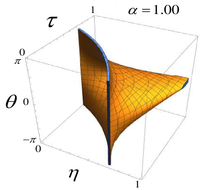
Figure 4: (Color online) Hong-Ou-Mandel manifold (HOMM) for $P_{c,d}(1,1)\leq 0.001$ for zero loss $\alpha=1$, as a function of through-coupling parameters $0\leq\tau\leq 1$ and $0\leq\eta\leq 1$ for the system output modes $c$ and $d$ respectively of Fig.(3), and the internal single round trip phase accumulation $-\pi\leq\theta\leq\pi$ (compare with Fig.(5b) of Hach III et al. (2014)).

As discussed in Hach et. al. Hach III et al. (2014), the two dimensional (three parameter) HOMM arising in the lossless add/drop ring resonator generalizes the zero dimensional (one parameter) Hong-Ou-Mandel effect C.K. Hong and Mandel (1987) where the single adjustable parameter is the transmissivity of the 50:50 beam splitter upon which the two photons interfere.

To examine the effects of coupling and intrinsic loss on the HOMM in the add/drop ring resonator, we begin with the input state $|1_{a},1_{b},0_{env}\rangle\equiv|1_{a},1_{b}\rangle\otimes|0\rangle_{env}$ where $|0\rangle_{env}$ represents the (for simplicity, zero temperature) initial vacuum state of the noise modes which are acted upon by the noise operators $\hat{f}_{a}$ and $\hat{f}_{b}$ defined in Eq.(24). Let us write Eq.(23) and Eq.(25) for the output modes $c$ and $d$ in terms of the system input modes $a$ and $b$ formally as

$$\hat{\vec{c}}_{out}=\left(\begin{array}[]{c}\hat{c}\\ \hat{d}\\ \end{array}\right)=\left(\begin{array}[]{cc}\mathcal{A}_{a\rightarrow c}&\mathcal{A}_{b\rightarrow c}\\ \mathcal{A}_{a\rightarrow d}&\mathcal{A}_{b\rightarrow d}\\ \end{array}\right)\,\left(\begin{array}[]{c}\hat{a}\\ \hat{b}\\ \end{array}\right)+\left(\begin{array}[]{c}\hat{F}_{c}\\ \hat{F}_{d}\\ \end{array}\right)\equiv M\,\hat{\vec{a}}_{in}+\hat{\vec{F}},$$ (26)

where we have defined the collective noise operators $\hat{F}_{c}=-i\,\sqrt{{\Gamma}}\,\left(|{\kappa}|^{2}\,\eta^{*}{\hat{f}}_{a}+{\gamma}^{*}\,{\kappa}{\hat{f}}_{b}\right)$, and $\hat{F}_{d}=-i\,\sqrt{{\Gamma}}\,\left({\kappa}^{*}\,{\gamma}{\hat{f}}_{a}+|{\gamma}|^{2}\,{\tau^{*}}{\hat{f}}_{b}\right)$. From the definition Eq.(24) we see that $\hat{f}_{a}$ depends on an integer number of round trip losses in the ring resonator (i.e. mode $\hat{a}\rightarrow\hat{c}$ or $\hat{b}\rightarrow\hat{d}$ involving the noise operator $\hat{s}_{n+1}(z,\omega)$), while $\hat{f}_{b}$ depends on an integer plus half number of round trip losses (i.e. mode $\hat{a}\rightarrow\hat{d}$ or $\hat{b}\rightarrow\hat{c}$ involving the noise operator $\hat{s}_{n+1/2}(z,\omega)$). Thus, while $[\hat{f}_{a},\hat{f}_{b}]=0$, we have $[\hat{f}_{a},\hat{f}^{\dagger}_{b}]\neq 0$. This is to be expected Barnett et al. (1996); Huang and Agarwal (2014) due to the feedback (sum over multiple round trips) provided by the ring resonator. While the commutator $[\hat{f}_{a},\hat{f}^{\dagger}_{b}]$ could be explicitly computed directly as in Section D (for the single bus ring resonator) we can now invoke (as is typically done) the unitarity of the input modes and output modes commutators to determine the value of the noise commutators. Returning to Eq.(26) in terms of the collective noise modes $\hat{F}_{c}$ and $\hat{F}_{d}$ we can infer that

$$[\hat{c}({\omega}),\hat{c}^{\dagger}({\omega}^{\prime})]=\delta({\omega}-{\omega}^{\prime}) \Rightarrow [\hat{F}_{c}({\omega}),\hat{F}_{c}^{\dagger}({\omega}^{\prime})]=\left(1-(|\mathcal{A}_{a\rightarrow c}|^{2}+|\mathcal{A}_{b\rightarrow c}|^{2})\right)\,\delta({\omega}-{\omega}^{\prime}),$$ (27a)

$${}[\hat{d}({\omega}),\hat{d}^{\dagger}({\omega}^{\prime})]=\delta({\omega}-{\omega}^{\prime}) \Rightarrow [\hat{F}_{d}({\omega}),\hat{F}_{d}^{\dagger}({\omega}^{\prime})]=\left(1-(|\mathcal{A}_{a\rightarrow d}|^{2}+|\mathcal{A}_{b\rightarrow d}|^{2})\right)\,\delta({\omega}-{\omega}^{\prime}),$$ (27b)

$${}[\hat{c}({\omega}),\hat{d}^{\dagger}({\omega}^{\prime})]=0 \Rightarrow [\hat{F}_{c}({\omega}),\hat{F}_{d}^{\dagger}({\omega}^{\prime})]=-\left(\mathcal{A}_{a\rightarrow c}\,\mathcal{A}^{*}_{a\rightarrow d}\,+\mathcal{A}_{b\rightarrow c}\,\mathcal{A}^{*}_{a\rightarrow d}\right)\,\delta({\omega}-{\omega}^{\prime}).$$ (27c)

The input state $|\Psi\rangle_{in}=|1_{a},1_{b},0_{env}\rangle={\hat{a}}^{\dagger}{\hat{b}}^{\dagger}|0_{a},0_{b},0_{env}\rangle$ is converted to the output state $|\Psi\rangle_{out}$ by rewriting the input modes operators $\hat{a}^{\dagger}$ and $\hat{b}^{\dagger}$ in terms of the output mode operators $\hat{c}^{\dagger}$ and $\hat{d}^{\dagger}$. Inverting Eq.(26) as

$$\hat{\vec{a}}^{\dagger}_{in}={\mathcal{M}}\,(\hat{\vec{c}}^{\dagger}_{out}-\hat{\vec{F}}^{\dagger}),\qquad{\mathcal{M}}=M^{-1*},$$ (28)

yields the output state

$$|\Psi\rangle_{out}\equiv|\Psi^{(2)}\rangle_{c,d}\otimes|0\rangle_{env}+|\phi^{(1)}\rangle_{c,d}\otimes\hat{F}_{c}^{\dagger}|0\rangle_{env}+|\varphi^{(1)}\rangle_{c,d}\otimes\hat{F}_{d}^{\dagger}|0\rangle_{env}+|0,0\rangle_{c,d}\otimes|\Phi^{(2)}\rangle_{env},$$ (29)

where

$$|\Psi^{(2)}\rangle_{c,d} = \sqrt{2}\,\mathcal{M}_{11}\,\mathcal{M}_{21}|2,0\rangle_{c,d}+\textrm{Perm}(\mathcal{M})\,|1,1\rangle_{c,d}+\sqrt{2}\,\mathcal{M}_{12}\,\mathcal{M}_{22}|0,2\rangle_{c,d},\quad$$ (30a)

$$|\phi^{(1)}\rangle_{c,d} = -\left(2\,\mathcal{M}_{11}\,\mathcal{M}_{21}|1,0\rangle_{c,d}+\textrm{Perm}(\mathcal{M})\,|0,1\rangle_{c,d}\right),$$ (30b)

$$|\varphi^{(1)}\rangle_{c,d} = -\left(\textrm{Perm}(\mathcal{M})\,|1,0\rangle_{c,d}+2\,\mathcal{M}_{12}\,\mathcal{M}_{22}|0,1\rangle_{c,d}\right),$$ (30c)

$$|\Phi^{(2)}\rangle_{env} = (\mathcal{M}_{11}\hat{F}_{c}^{\dagger}+\mathcal{M}_{12}\hat{F}_{d}^{\dagger})\,(\mathcal{M}_{21}\hat{F}_{c}^{\dagger}+\mathcal{M}_{22}\hat{F}_{d}^{\dagger})\,|0\rangle_{env},$$ (30d)

where we have defined

$$\textrm{Perm}(\mathcal{M})\equiv\mathcal{M}_{11}\,\mathcal{M}_{22}+\mathcal{M}_{12}\,\mathcal{M}_{21},$$ (31)

as the permanent Scheel (2008); *Scheel:2004 of the matrix $\mathcal{M}$.

Ultimately we are interested in the observable reduced system density matrix $\rho_{c,d}=\textrm{Tr}_{env}[|\Psi\rangle_{out}\langle\Psi|]$ of the output modes $c$ and $d$. The trace over the environment is facilitated by the observation that e.g. $\textrm{Tr}_{env}[\hat{F}_{i}^{\dagger}|0\rangle_{env}\langle 0|\hat{F}_{j}]={}_{env}\langle 0|\hat{F}_{j}\,\hat{F}_{i}^{\dagger}|0\rangle_{env}={}_{env}\langle 0|[\hat{F}_{j},\hat{F}_{i}^{\dagger}]+\hat{F}_{i}^{\dagger}\,\hat{F}_{j}|0\rangle_{env}=[\hat{F}_{j},\hat{F}_{i}^{\dagger}]$ for $i,j\in\{c,d\}$ and where use of Eq.(27a), Eq.(27b), and Eq.(27c) can be made.

The reduced system density matrix has the form

$$\rho_{c,d}=\sum_{k=\{0,1,2\}}\,p_{k}\,\rho^{(k)}_{c,d},\qquad\textrm{Tr}_{c,d}[\rho^{(k)}_{c,d}]=1,\qquad\sum_{k=\{0,1,2\}}\,p_{k}=1,$$ (32)

where the index $k$ labels the number of photons in the modes $c$ and $d$. The 2-system-photon sector $\rho^{(2)}_{c,d}$ is spanned by the states $\{|2,0\rangle_{c,d},|1,1\rangle_{c,d},|0,2\rangle_{c,d}\}$, the 1-system-photon sector $\rho^{(1)}_{c,d}$ is spanned by the states $\{|1,0\rangle_{c,d},|0,1\rangle_{c,d}\}$, and the the 0-system-photon sector $\rho^{(0)}_{c,d}$ is the vacuum state $|0\rangle_{c,d}\langle 0|$.

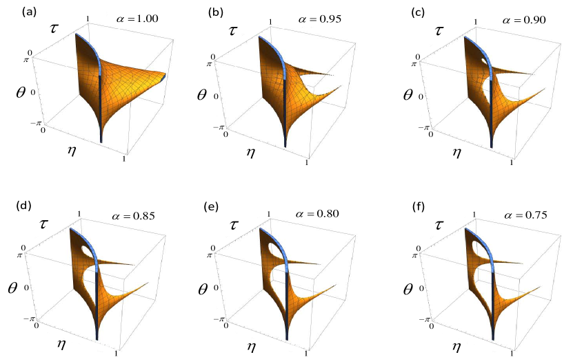
Figure 5: (Color online) Hong-Ou-Mandel manifold (HOMM) for $0\leq P^{(\alpha)}_{c,d}(1,1)\leq 0.001$ as a function of the loss parameter $\alpha=e^{-{\Gamma}L/2}$, the through-coupling parameters $0\leq\tau\leq 1$ and $0\leq\eta\leq 1$ for the system output modes $c$ and $d$ respectively of Fig.(3), and the internal single round trip phase accumulation $-\pi\leq\theta\leq\pi$. (a) $\alpha=1.0$ (lossless), (b) $\alpha=0.95$, (c) $\alpha=0.90$, (d) $\alpha=0.85$, (e) $\alpha=0.80$, (f) $\alpha=0.75$ (compare with Fig.(4)).

Finally, $P_{c,d}^{(\alpha)}(1,1)\equiv{}_{c,d}\langle 1,1|\rho^{(1)}_{c,d}|1,1\rangle_{c,d}$ is the probability, as function of the loss parameter $\alpha=e^{-{\Gamma}L/2}$, that a coincidence detection will contain one output photon in mode $c$ and one output photon in mode $d$ for the diagonal density matrix $\rho^{(1)}_{c,d}$. (Such events occur randomly with probability $p_{2}$). From Eq.(30a) we see that $P_{c,d}^{(\alpha)}(1,1)=\textrm{Perm}(\mathcal{M})$ as has been recently noted in the theory of generalized multiphoton (i.e HOM) quantum interference effects, especially in regards to the problem of boson sampling Tan et al. (2013); *Sanders:2014; *Sanders:2015; *Tichy:2015.

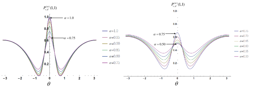
Figure 6: (Color online) Hong-Ou-Mandel manifold (HOMM) for $P^{(\alpha)}_{c,d}(1,1)=0$ for the important special case of critical coupling $\tau=\eta=1/\sqrt{2}$ (i.e. 3dB couplers) versus the internal single round trip phase accumulation $-\pi\leq\theta\leq\pi$ for various loss parameters $\alpha=e^{-{\Gamma}L/2}$. (left) $0.75\leq\alpha\leq 1.0$, (right) $0.50\leq\alpha\leq 0.75$ (compare Fig.(6b) of Hach III et al. (2014)).

The expression for $P_{c,d}^{(\alpha)}(1,1)$ is given by

$$P_{c,d}^{(\alpha)}(1,1)=$$

$$\frac{(|\tau|^{2}+\alpha^{2}\,|\eta|^{2}-\alpha\,r)\,(|\eta|^{2}+\alpha^{2}\,|\tau|^{2}-\alpha\,r)+\alpha^{2}\,|\kappa|^{4}\,|\gamma|^{4}+\alpha\,|\kappa|^{2}\,|\gamma|^{2}\,\left((1+\alpha^{2})\,r-2\alpha(|\tau|^{2}+|\eta|^{2})\right)}{(|\tau|^{2}+\alpha^{2}\,|\eta|^{2}-\alpha\,r)\,(|\eta|^{2}+\alpha^{2}\,|\tau|^{2}-\alpha\,r)+\alpha^{2}\,|\kappa|^{4}\,|\gamma|^{4}-\alpha\,|\kappa|^{2}\,|\gamma|^{2}\,\left((1+\alpha^{2})\,r-2\alpha(|\tau|^{2}+|\eta|^{2})\right)},\qquad$$ (33)

where we have defined $r\equiv 2\,\textrm{Re}(\tau\eta\,e^{-i\theta})$. Eq.(IV) reduces in the lossless case $\alpha=1$ to

$$P_{c,d}^{(\alpha=1)}(1,1)=\left(\frac{|\tau|^{2}+|\eta|^{2}-r-|\kappa|^{2}\,|\gamma|^{2}}{|\tau|^{2}+|\eta|^{2}-r+|\kappa|^{2}\,|\gamma|^{2}}\right)^{2}$$ (34)

whose numerator (set equal to zero) was examined in Hach III et al. (2014) for the case of the lossless HOMM.

In Fig.(5) we plot the region $0\leq P_{c,d}(1,1)\leq 0.001$ corresponding to $99.9\%$ eps destructive interference of the quantum amplitude for the state $|1_{c},1_{d}\rangle$ for the real parameters $0\leq\tau,\eta\leq 1$ (with the cross-coupling parameters giving by $\kappa=\sqrt{1-\tau^{2}}$ and $\gamma=\sqrt{1-\eta^{2}}$) and $-\pi\leq\theta\leq\pi$. The HOMM begins to break up at approximately $5\%$ loss ($\alpha=0.95$), and reduces to essentially a lower dimension manifold for loss greater than $10\%$ ($\alpha<0.90$). Currently, loss in silicon ring resonators at $1550$nm can be as low as $1\%$ Hach III et al. (2016); Preble et al. (2015) so that the observation of the HOMM appears experimentally feasible.

In Fig.(6) we plot $P^{(\alpha)}_{c,d}(1,1)=0$ for the important special case of critical coupling $\tau=\eta=1/\sqrt{2}$ (i.e. 3dB couplers) versus the internal single round trip phase accumulation $\theta$ for various loss parameters $0.5\leq\alpha\leq 1.0$. As the internal and coupling loss (${\Gamma}$) increases ($\alpha=e^{-{\Gamma}L/2}$ decreases) we observe the expected disappearance of the HOM dip (zero minima for the lossless case $\alpha=1.0$) and the decrease in visibility (difference between maximum value at $\theta=0$ and minimum values of $P^{(\alpha)}_{c,d}(1,1)=0$). Again, we can see that for up to $5\%$ loss ($0.95\leq\alpha\leq 1.0$) the observation of the HOMM appears experimentally feasible.

It is also interesting to examine the one system photon sector $\rho^{(1)}_{c,d}$ of the reduced density matrix $\rho_{c,d}$ spanned by the basis states $\{|1,0\rangle_{c,d},|0,1\rangle_{c,d}\}$. Let us define the un-normalized state $\tilde{\rho}^{(1)}_{c,d}$ as

$$\tilde{\rho}^{(1)}_{c,d}=|\phi^{(1)}\rangle_{c,d}\langle\phi^{(1)}|\,[\hat{F}_{c},\hat{F}_{c}^{\dagger}]+|\phi^{(1)}\rangle_{c,d}\langle\varphi^{(2)}|\,[\hat{F}_{d},\hat{F}_{c}^{\dagger}]+|\varphi^{(2)}\rangle_{c,d}\langle\phi^{(1)}|\,[\hat{F}_{c},\hat{F}_{d}^{\dagger}]+|\varphi^{(2)}\rangle_{c,d}\langle\varphi^{(2)}|\,[\hat{F}_{d},\hat{F}_{d}^{\dagger}],\qquad$$ (35)

and $p_{1}=\textrm{Tr}[\tilde{\rho}^{(1)}_{c,d}]$, then $\rho^{(1)}_{c,d}=\tilde{\rho}^{(1)}_{c,d}/p_{1}$. Note that $\rho^{(1)}_{c,d}=\textrm{Tr}[|\Psi^{(1)}\rangle_{out}\,\langle\Psi^{(1)}|]$ arises from the trace over the environment of the (post-selected) one system photon portion of $|\Psi_{out}\rangle$ in Eq.(29) where

$$|\Psi^{(1)}\rangle_{out}\equiv\frac{1}{\sqrt{p_{1}}}\,\left(|\phi^{(1)}\rangle_{c,d}\otimes\hat{F}_{c}^{\dagger}|0\rangle_{env}+|\varphi^{(1)}\rangle_{c,d}\otimes\hat{F}_{d}^{\dagger}|0\rangle_{env}\right),$$ (36)

and hence $|\Psi^{(1)}\rangle_{out}$ could be considered as the (system-environment) purification of the (post-selected, with probability $p_{1}$) system state $\rho^{(1)}_{c,d}$. As such, the entropy $S^{(1)}=-\textrm{Tr}[\,\rho^{(1)}_{c,d}\,\log_{2}\,\rho^{(1)}_{c,d}\,]$ indicates a measure of the bipartite entanglement between the system and environment for the post-selected state $|\Psi^{(1)}\rangle_{out}$.

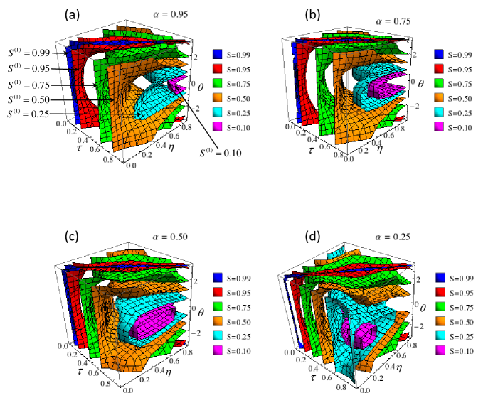
Figure 7: (Color online) Contour plots of the von Neumann entropy $S^{(1)}=-\textrm{Tr}[\,\rho^{(1)}_{c,d}\,\log_{2}\,\rho^{(1)}_{c,d}\,]$ for the one system photon sector of $\rho_{c,d}$ as a function of through-coupling parameters $0\leq\tau\leq 1$ and $0\leq\eta\leq 1$, and the internal single round trip phase accumulation $-\pi\leq\theta\leq\pi$, for various loss parameters $\alpha=e^{-{\Gamma}L/2}$. (a) $\alpha=0.95$, (b) $\alpha=0.75$, (c) $\alpha=0.50$, (d) $\alpha=0.25$. (Surface manifolds for contour values of $S^{(1)}\in\{0.99,0.95,0.75,0.50,0.25,0.10\}$ retain the same nested relative orientation (from left to right) for all subplots $(a)-(d)$ as that labeled in $(a)$).

In Fig.(7) we plot level surfaces of $S^{(1)}$ as a function of $\tau$, $\eta$ and $\theta$ for various values of the loss parameter $\alpha$. Values of $S^{(1)}$ closer to unity indicate greater entanglement between single system photon (in mode $c$ and $d$), and the single photon lost to the environment in the post-selected state $|\Psi^{(1)}\rangle_{out}$. These regions of larger entanglement are diminished as loss is increased ($\alpha$ decreased).

Lastly, it is interesting to note that from the definition of $|\phi^{(1)}\rangle_{c,d}$ in Eq.(30b) and $|\varphi^{(1)}\rangle_{c,d}$ in Eq.(30c) that both states are suppositions of the one system photon basis states $\{|1,0\rangle_{c,d},|0,1\rangle_{c,d}\}$. These superpositions are completely destroyed precisely at the condition that HOMM is strongest, namely $P^{(\alpha)}_{c,d}(1,1)=\textrm{Perm}(\mathcal{M})=0$.

V Summary and Outlook

In this paper we have examined quantum optical losses in ring resonators using field operator transformations. Specifically, we have demonstrated the equivalence between our operator valued phasor addition of ‘Feynman paths’ circulating within the resonator and the more standard Langevin approach. In fact, we have shown that the OVPA approach we present here is slightly more general in that it is valid for all frequencies of light while the Langevin only holds near a resonance of the system. This result represents an important ‘unification’ of the description of such networks based upon scattering theory with that based upon quantum transfer functions (matrices). With the results of this paper in place, we can now investigate the quantum optical response of ring resonator networks to exotic states of light in the presence of losses We will apply the techniques developed here and elsewhere in the references to design and optimize silicon nanophotonic networks for quantum information processing, optical metrology, and communication.

Note, after the completion of this work, the authors were made aware of the paper by Raymer and McKinstrie (2013) Raymer and McKinstrie (2013) which considered a generalization of the standard Langevin input-output formalism that explicitly takes into account circulation factors accounting for the multiple round trips of the fields inside a cavity or ring resonator. That work considered an equation of motion for one round trip of a single bus cavity field with no internal losses, along with auxiliary beam-splitter like boundary conditions relating the input and output fields to the circulating cavity field. While not explicitly including internal propagation losses, the authors indicated how they would be included in a Langevin approach. The current work discussed in this paper is similar in spirit, but considers directly the total summation of all round trip circulations of the field(s) in a lossy (coupling and propagation) single bus and dual bus ring resonator without the use of boundary conditions. The two approaches are equivalent to each other. Both works consider the agreement of the formalism with the standard Langevin approach in the high cavity Q limit.

Appendix A Classical derivation of input-output fields

In the interest of making this paper as self-contained as possible, we review in this appendix the classical derivation of the input-output formalism by Haus Haus (1984); Little et al. (1997); Haus (2000), relating the coupling of an internal cavity (complex) amplitude $a_{int}$ to an external input $a_{in}$ and output field $a_{out}$ as illustrated in Fig.(8). Since the optical system considered here is linear, the classical equations will also hold in the quantum regime, as will be reviewed in the next appendix, where consideration of commutation relations must be additionally taken into account. The phenomenological derivation by Haus relies on three principles (i) energy conservation, (ii) time reversibility and (iii) perturbation theory to formulate a dynamical, and boundary condition relation between the internal cavity and the external driving and out-coupled modes.

A.1 A single cavity resonance

The equation of motion for the internal field $a_{int}$ in a one-sided lossy Fabry-Perot cavity, as illustrated in Fig.(8), driven by an external field $a_{in}$ and out-coupled to the external field $a_{out}$ is given by,

$$\dot{a}_{int}=-(i\,\omega_{0}+\gamma_{c}/2+\gamma_{int}/2)\,a_{int}+\sqrt{\gamma_{c}}\,a_{in}.$$ (37)

Figure 8: One-sided cavity with classical input field amplitude $a_{in}$, output field $a_{out}$ and internal cavity field $a_{int}$. $\gamma_{c}$ is the (power) decay rate of the internal field to the external field through the mirror. $\gamma_{int}$ represents internal losses within the cavity.

Here, $\omega_{0}$ is the resonance frequency of the undriven cavity, $\gamma_{c}$ is the power decay rate of the internal field through the partial mirror to the external mode $(d|a_{int}|^{2}/dt=-\gamma_{c}\,a_{int})$, and $\gamma_{int}$ describes internal (e.g. scattering) losses within the cavity. The term $\sqrt{\gamma_{c}}\,a_{in}$ describes the in-coupling of the form $\kappa\,a_{in}$ of the external field of complex amplitude $a_{in}$ with coupling constant $\kappa$. One can relate the coupling constant $\kappa$ to the cavity decay rate $\gamma_{c}$ through energy conservation and time reversal as $\kappa^{2}=\gamma_{c}$ (for detailed derivation see Haus Haus (1984); Little et al. (1997); Haus (2000)). For a driving field excitation $a_{in}$ proportional to $e^{-i\omega\,t}$, the internal field has the solution,

$$a_{int}=\frac{\kappa\,a_{in}}{\gamma_{c}/2+\gamma_{int}/2-i\,(\omega-\omega_{0})}.$$ (38)

describing a complex Lorentzian form of width $(\gamma_{c}+\gamma_{int})/2$.

One can relate the output field $a_{out}$ to the input $a_{in}$ and internal cavity field $a_{int}$ through power conservation (in appropriately normalized units of energy and power),

$$|a_{in}|^{2}-|a_{out}|^{2}=\frac{d|a_{int}|^{2}}{dt}=-\gamma_{c}\,|a_{int}|^{2}+\sqrt{\gamma_{c}}\,(a_{in}\,a^{*}_{int}+a^{*}_{in}\,a_{int}).$$ (39)

Since the system is linear we can write formally the ansatz $a_{out}=c_{in}\,a_{in}+c_{int}\,a_{int},$ for some complex constants $c_{in}$ and $c_{int}$. From the case of the undriven cavity with no internal losses ($a_{in}=\gamma_{int}=0$), energy conservation $d|a_{int}|^{2}/dt=-\gamma_{c}\,|a_{int}|^{2}=-|a_{out}|^{2}$ yields $a_{out}=\sqrt{\gamma_{c}}\,a_{int}$ so that $c_{int}=\sqrt{\gamma_{c}}$. Substituting $a_{out}=c_{in}\,a_{in}+\sqrt{\gamma_{c}}\,a_{int}$ into the left hand side of the above ansatz produces $|a_{in}|^{2}\,(c_{int}+1)-\gamma_{c}\,|a_{int}|^{2}-\sqrt{\gamma_{c}}\,(c_{in}\,a_{in}\,a^{*}_{int}+c^{*}_{in}\,a^{*}_{in}\,a_{int})$ which on comparison with the right hand side of Eq.(39) yields the real solution $c_{int}=-1$. Thus, we obtain,

$$a_{out}=-a_{in}+\sqrt{\gamma_{c}}\,a_{int},\quad\textrm{or}\quad a_{in}+a_{out}=\sqrt{\gamma_{c}}\,a_{int},$$ (40)

which can be considered as a boundary condition for the fields at the lossy mirror.

Using Eq.(38) and the boundary condition Eq.(40) we can calculate the reflection coefficient $r$ as,

$$r=\frac{a_{out}}{a_{in}}=\frac{\sqrt{\gamma_{c}}\,a_{int}-a_{in}}{a_{in}}=\frac{(\gamma_{c}-\gamma_{int})/2+i(\omega-\omega_{0})}{(\gamma_{c}+\gamma_{int})/2-i(\omega-\omega_{0})}\equiv\frac{\gamma_{-}+i\delta}{\gamma_{+}-i\delta},$$ (41)

where in the last equality we have defined $\gamma_{\pm}=(\gamma_{c}\pm\gamma_{int})/2$ and $\delta=\omega-\omega_{0}$, as in the main body. Note that when the internal losses are zero $\gamma_{int}=0$ one has $|r|=1$, otherwise $|r|<1.$ Eq.(37) and the boundary condition Eq.(40) describe the internal classical field amplitude $a_{int}$ of the resonator near a single resonance and relates it to the input driving field $a_{in}$ and the external traveling wave mode $a_{out}$ that it couples to. Since the systems is linear, these equations also hold in the quantum regime, as will be shown in the next appendix, where consideration of commutation relations must be taken into account.

A.2 Extension to internal losses and multiple resonances

The generalization to multiple resonances is achieved by writing Eq.(37) for each internal cavity mode $a_{int,j}$ near resonance frequency $\omega_{0,j}$, with individual coupling $\gamma_{c,j}$ and internal losses $\gamma_{int,j}$,

$$\dot{a}_{int,j}=-(i\,\omega_{0,j}+\gamma_{c,j}/2+\gamma_{int,j}/2)\,a_{int,j}+\sqrt{\gamma_{c,j}}\,a_{in}.$$ (42)

The boundary condition Eq.(40) generalizes to,

$$a_{out}=c_{in}\,a_{in}+\sum_{j}\,\sqrt{\gamma_{c,j}}\,a_{int,j}.$$ (43)

The reflection coefficient similarly generalizes to,

$$r=\frac{a_{out}}{a_{in}}=c_{in}+\sum_{j}\,\frac{\gamma_{c,j}}{(\gamma_{c,j}+\gamma_{int,j})/2-i(\omega-\omega_{0,j})},\equiv c_{in}+\sum_{j}\,L_{j},$$ (44)

where we have defined the complex Lorentzian $L_{j}=\gamma_{c,j}/[\gamma_{c,j}+\gamma_{int,j})/2-i(\omega-\omega_{0,j})]$. Again, for zero internal losses $\gamma_{int,j}=0$ we must have $|r|^{2}=1$ which leads to a quadratic equation for $c_{in}$ (taken as real),

$$(c_{in}+1)\,(c_{in}-1)+(c_{in}+1)\,\sum_{j}\,|L_{j}|^{2}+2\,\sum_{j\neq k}\,\textrm{Re}(L_{j}\,L^{*}_{k})=0.$$ (45)

We see that $c_{in}$ is now a function of $\omega$. For a single resonance $j=1$ there is only one term in the sum $\sum_{j}L_{j}$ and hence the last term in Eq.(45) is not present. By inspection, $c_{in}=-1$ in this case. For the general case, near a particular resonance $\omega=\omega_{j}+\Omega$ such that $\Omega,\gamma_{c,j}\ll|\omega_{j}-\omega_{k}|$ for $k\neq j$ (i.e. well separated resonances, large free spectral range) $|L_{k\neq j}|\approx\gamma_{c,k}/|\omega_{j}-\omega_{k}|\ll 1$ so that the last cross term in Eq.(45) is negligible and only the single $|L_{j}|^{2}$ term contributes to the middle sum. Hence, as in the single resonance case Eq.(45) becomes approximately $(c_{in}+1)\,(c_{in}-1)+(c_{in}+1)\,|L_{j}|\approx 0$ with solution $c_{in}(\omega_{j}+\Omega)\approx-1$. Thus, near each individual resonance, the single resonance boundary condition Eq.(40) holds.

Appendix B Quantum derivation of input-output fields

The quantum derivation of the input-output relations for optical fields in a cavity is attributed to the work of Collett and Gardiner Collet and Gardiner (1984). Here we follow the often cited texts of Walls and Milburn Walls and Milburn (1994) and of Orszag Orszag (2000). In this formulation a Hamiltonian is prescribed to yield dynamics of the same form given classically in Eq.(37) due to the linearity of the system. The quantum version of the classical boundary condition Eq.(40) arises from the difference between the equations of motion for the noise operators considered in the far past and far future, which couples the internal cavity mode to the external modes of the cavity. The essential new feature of the quantum derivation is the preservation of the commutation relations of all involved operators, which is required by the unitarity of the quantum evolution. While this material is now standard in quantum optics canon, we include it here for completeness, and for comparison to the OVPA coupling derivation used in the main body of the text.

Figure 9: Same one sided cavity as in Fig.(8), except now classical amplitudes have been changed to quantum fields.

The quantum input-output relations are instantiations of the $S$ (scattering) matrix which relates input fields to output fields. Here we assume linear interactions between the system and the bath, the rotating wave approximation and that the spectrum of the bath is flat, independent of frequency. The Hamiltonian is given by,

$$H = H_{sys}+H_{B}+H_{INT},$$ (46a)

$$H_{B} = \int_{-\infty}^{\infty}d\omega\,\hbar\,\omega\,\hat{b}^{\dagger}(\omega)\,\hat{b}(\omega),$$ (46b)

$$H_{int} = i\,\hbar\int_{-\infty}^{\infty}d\omega\,\kappa(\omega)\,\left(\hat{b}^{\dagger}(\omega)\,\hat{a}_{int}-\hat{b}(\omega)\,\hat{a}^{\dagger}_{int}\right).$$ (46c)

Here $\hat{a}_{int}$ is the internal cavity mode, $\hat{b}^{\dagger}(\omega),\,\hat{b}(\omega)$ are the creation and annihilation operator for the bath modes assumed to have a white noise spectrum such that $[\hat{b}(\omega),\,\hat{b}^{\dagger}(\omega^{\prime})]=\delta(\omega-\omega^{\prime})$, and $\kappa(\omega)$ is the coupling constant. Though the frequencies are positive, the integration range can be extended from $(-\omega_{0},\infty)$ in a rotating frame of frequency $\omega_{0}$. The lower limit of the integral can then be extended to $-\infty$ for $\omega_{0}\gg\Delta\omega$ where $\Delta\omega$ is the bandwidth of frequencies under consideration (say, near a particular resonance).

The Heisenberg equations of motion yield,

$$\dot{\hat{b}}(\omega,t) = -i\,\omega\,\hat{b}(\omega,t)+\kappa(\omega)\,\hat{a}_{int},$$ (47a)

$$\dot{\hat{a}}_{int}(\omega,t) = -\frac{i}{\hbar}\,[\hat{a}_{int},H_{sys}]-\int_{-\infty}^{\infty}d\omega\,\kappa(\omega)\,\hat{a}_{int}.$$ (47b)

We can solve Eq.(47a) for $\hat{b}(\omega,t)$ depending on two different choices of the initial conditions,

$$\hat{b}(\omega,t) = e^{-i\omega(t-t_{0})}\,\hat{b}(\omega,t_{0})+\int_{t_{0}}^{t}dt^{\prime}\,\kappa(\omega)\,e^{-i\omega(t-t^{\prime})}\,\hat{a}_{int}(t^{\prime}),$$ (48a)

$$\hat{b}(\omega,t) = e^{-i\omega(t-t_{1})}\,\hat{b}(\omega,t_{1})-\int_{t}^{t_{1}}dt^{\prime}\,\kappa(\omega)\,e^{-i\omega(t-t^{\prime})}\,\hat{a}_{int}(t^{\prime}).$$ (48b)

In Eq.(48a) the initial condition has been chosen at a time in the far past $t_{0}<t$ such that $b(\omega,t_{0})$ represents the bath operators at very early times (often taken to be $t_{0}=-\infty$), whereas in Eq.(48b) the initial condition has been chosen to be in the far future $t_{1}>t$ such that $b(\omega,t_{1})$ represents the bath operators at very late times (often taken to be $t_{1}=\infty$). We also assume that in the far past, the bath and the system are uncorrelated so that the operators commute $[a_{int},b(\omega,t_{0})]=[a_{int},b^{\dagger}(\omega,t_{0})]=0$.

We first consider the substitution of Eq.(48a) into Eq.(47b) to obtain the exact equation,

$$\dot{a}_{int}(t) = -\frac{i}{\hbar}\,[\hat{a}_{int},H_{sys}]$$ (49a)

$$- \int_{-\infty}^{\infty}d\omega\,\kappa(\omega)\,e^{-i\omega(t-t_{0})}\,\hat{b}(\omega,t_{0}),$$

$$- \int_{-\infty}^{\infty}d\omega\,\kappa^{2}(\omega)\,\int_{t_{0}}^{t}dt^{\prime}\,\,e^{-i\omega(t-t_{0})}\,\hat{a}_{int}(t^{\prime}).$$ (49b)

We now invoke the Markov approximation that coupling $\kappa(\omega)$ is constant over the bandwidth $\Delta\omega$ so that we can pull it out from under the integral in term (49a). As in Appendix A we relate the coupling constant $\kappa(\omega)$ to the cavity decay rate $\gamma_{c}$ via $\kappa^{2}(\omega)=\gamma_{c}/(2\pi)$. We further define the remaining integral in term (49a) as,

$$\hat{a}_{in}(t)\equiv-\frac{1}{\sqrt{2\pi}}\,\int_{-\infty}^{\infty}d\omega\,e^{-i\omega(t-t_{0})}\,\hat{b}(\omega,t_{0}),$$ (50)

using the sign convention that incoming fields to the cavity have a minus sign, while outgoing fields have a plus sign (see $a_{out}(t)$ below. Thus, the term (49a) becomes $\sqrt{\gamma_{c}}\,\hat{a}_{in}(t)$. By use of the definition and properties of the delta function,

$$\frac{1}{2\pi}\,\int_{-\infty}^{\infty}d\omega\,e^{-i\omega(t-t^{\prime})} = \delta(t-t^{\prime}),$$ (51a)

$$\int_{t_{0}}^{t}dt^{\prime}\,f(t^{\prime})\,\delta(t-t^{\prime})=\int_{t}^{t_{1}}dt^{\prime}\,f(t^{\prime})\,\delta(t-t^{\prime}) = \frac{1}{2}\,f(t),\quad t_{0}<t<t_{1},$$ (51b)

and the initial bath operator equal time commutation relations $[\hat{b}(\omega,t_{0}),\hat{b}^{\dagger}(\omega^{\prime},t_{0})]=\delta(\omega-\omega^{\prime})$, one has

$$[\hat{a}_{in}(t),\hat{a}^{\dagger}_{in}(t^{\prime})]=\delta(t-t^{\prime}).$$ (52)

By again pulling out $\kappa(\omega)=\gamma_{c}/(2\pi)$ from under the integral in Eq.(49b) and using Eq.(51a) and Eq.(51b) the term in Eq.(49b) becomes $-\gamma_{c}/2\,a_{int}(t)$. Gathering these results together yields the equation for the internal cavity mode $\hat{a}_{int}(t)$,

$$\dot{\hat{a}}_{int}(t)=-\frac{i}{\hbar}\,[\hat{a}_{int},H_{sys}]-\frac{\gamma_{c}}{2}\,\hat{a}_{int}(t)+\sqrt{\gamma_{c}}\,\hat{a}_{in}(t).$$ (53)

This is the exact same form as the classical equation of motion for $a_{int}$ in Eq.(37) if we take $H_{sys}=\hbar\omega_{0}\,\hat{a}^{\dagger}_{int}\,\hat{a}_{int}$ as the free-field, empty cavity Hamiltonian, and consider no internal losses $\gamma_{int}=0$. Eq.(53) is the quantum Langevin Walls and Milburn (1994); Mandel and Wolf (1995); Scully and Zubairy (1997); Orszag (2000) equation of motion for the internal cavity mode $\hat{a}_{int}$ coupled to the input driving field $\hat{a}_{in}$. It is an embodiment of the fluctuation-dissipation theorem Mandel and Wolf (1995) which states that effect of loss (dissipation) in the system is accompanied by the presence of noise sources (fluctuations) as the cause of the loss. These noise operators must be present quantum mechanically in order to preserve the system commutation relations $[\hat{a}_{int}(t),\hat{a}^{\dagger}_{int}(t^{\prime})]=\delta(t-t^{\prime})$. Otherwise, without the presence of the term $\hat{a}_{in}(t)$ in Eq.(53) the system commutator would decay to zero as $e^{-\gamma_{c}(t-t^{\prime})}$.

We can repeat the above development of the equation of motion for $\hat{a}_{int}$, this time using the solution for $\hat{b}(\omega,t)$ in Eq.(48b) in terms of the far-future modes $\hat{b}(\omega,t_{1})$ to obtain,

$$\dot{\hat{a}}_{int}(t)=-\frac{i}{\hbar}\,[\hat{a}_{int},H_{sys}]+\frac{\gamma_{c}}{2}\,\hat{a}_{int}(t)-\sqrt{\gamma_{c}}\,\hat{a}_{out}(t).$$ (54)

where we have defined $\hat{a}_{out}(t)$ analogous to Eq.(50) as,

$$\hat{a}_{out}(t)\equiv\frac{1}{\sqrt{2\pi}}\,\int_{-\infty}^{\infty}d\omega\,e^{-i\omega(t-t_{1})}\,\hat{b}(\omega,t_{1}),$$ (55)

which straightforwardly yields the commutation relations,

$$[\hat{a}_{out}(t),\hat{a}^{\dagger}_{out}(t^{\prime})]=\delta(t-t^{\prime}),$$ (56)

analogous to Eq.(52). Lastly, the boundary condition between the input, output and internal cavity mode is obtained by subtracting the two equations of motion for $\hat{a}_{int}(t)$ Eq.(53) and Eq.(54) to obtain,

$$\hat{a}_{in}(t)+\hat{a}_{out}(t)=\sqrt{\gamma_{c}}\,\hat{a}_{int}(t),$$ (57)

which has the exact same form as the classical boundary condition obtained in Eq.(40).

Although the above analysis pertains to cavities driven by a bath, it is not necessarily a theory about noise, since the only properties assumed about the bath is flat spectral response Orszag (2000). Similar to Eq.(37), we can explicitly include internal losses, treating $\hat{a}_{in}$ as an external (non-noise) driving field by explicitly including noise operators $\hat{f}(t)$ that are delta correlated in time $[\hat{f}(t),\hat{f}^{\dagger}(t^{\prime})]=\delta(t-t^{\prime})$,

$$\dot{\hat{a}}_{int}(t)=-\frac{i}{\hbar}\,[\hat{a}_{int},H_{sys}]-\frac{(\gamma_{c}+\gamma_{int})}{2}\,\hat{a}_{int}(t)+\sqrt{\gamma_{c}}\,\hat{a}_{in}(t)+\sqrt{\gamma_{int}}\,\hat{f}(t).$$ (58)

Appendix C Loudon’s quantum traveling-wave attenuation

One of the primary expressions we use in the main body of the paper is Loudon’s formulation for traveling-wave attenuation by an infinite series of discrete beam splitters. Here we summarize Loudon’s derivation Barnett et al. (1997); Loudon (2000) and note several important points on the commutation relations for the effective noise operator expressions.

To model loss in a quantized traveling wave field $\hat{a}$, Loudon considers successive propagation through an infinite series of fictitious beam splitters as illustrated in Fig.(10). For the $r$th beam splitter, $\hat{s}^{(in)}_{r}$ represents noise that is scattered into the beam by scattering centers,

Figure 10: Loudon’s traveling-wave attenuation by an infinite set of discrete beam splitters.

while $\hat{s}^{(out)}_{r}$ represents light that is scattered out of the beam. Each beam splitter (i.e. scattering center) is modeled by a frequency dependent transmission and reflection coefficient $T(\omega),\,R(\omega)$, respectively such that,

$$\hat{a}_{r+1}(\omega) = T(\omega)\,\hat{a}_{r}(\omega)+R(\omega)\,\hat{s}^{(in)}_{r}(\omega),$$ (59a)

$$\hat{s}^{(out)}_{r}(\omega) = R(\omega)\,\hat{a}_{r}(\omega)+T(\omega)\,\hat{s}^{(in)}_{r}(\omega).$$ (59b)

Here we assume that the pairs of input and output operators satisfy the usual boson commutation relations,

$$[\hat{a}_{r}(\omega),\hat{a}^{\dagger}_{r}(\omega^{\prime})]=[\hat{a}_{r+1}(\omega),\hat{a}^{\dagger}_{r+1}(\omega^{\prime})]=[\hat{s}^{(out)}_{r}(\omega),\hat{s}^{\dagger(out)}_{r}(\omega^{\prime})]=\delta(\omega-\omega^{\prime}).$$ (60)

and that operators for the different scattering sites are independent and obey,

$$[\hat{s}^{(in)}_{r}(\omega),\hat{s}^{\dagger(in)}_{r^{\prime}}(\omega^{\prime})]=\delta_{r,r^{\prime}}\,\delta(\omega-\omega^{\prime}).$$ (61)

Successive iteration of Eq.(59a) yields,

$$\hat{a}_{N+1}(\omega)=T^{N}(\omega)\,\hat{a}_{1}(\omega)+R(\omega)\,\sum_{r=1}^{N}T^{N-r}(\omega)\,\hat{s}^{(in)}_{r}(\omega).$$ (62)

We now take the continuum limit $N\to\infty$, $\Delta z=L/N\to 0$ and $|R(\omega)|^{2}\to 0$ and define the attenuation constant $\Gamma(\omega)=|R(\omega)|^{2}/\Delta z$. Using $|T(\omega)|^{2}+|R(\omega)|^{2}=1$ we have,

$$|T(\omega)|^{2N}=(1-|R(\omega)|^{2})^{N}=(1-\Gamma(\omega)L/N)^{N}\to e^{-\Gamma(\omega)L},$$ (63)

for which we take,

$$T(\omega)=e^{i\,n(\omega)(\omega/c)-\frac{1}{2}\Gamma(\omega)\,\Delta z}\equiv e^{i\xi(\omega)\Delta z},\quad\xi(\omega)\equiv\beta(\omega)+i\Gamma(\omega)/2,\quad\beta(\omega)\equiv n(\omega)(\omega/c).$$ (64)

In Eq.(64) we have chosen the phase of $T(\omega)$ to incorporate the free propagation constant $\beta(\omega)\equiv n(\omega)(\omega/c)$ through a medium of index of refraction $n(\omega)$, and defined the complex propagation constant as $\xi(\omega)\equiv\beta(\omega)+i\Gamma(\omega)/2$. We use $(N-r)\Delta z=L-z$ and convert from discrete to continuous modes through the identification,

$$\hat{s}^{(in)}_{r}(\omega)\to(\Delta z)^{1/2}\hat{s}(z,\omega),\quad\delta_{r,r^{\prime}}\to\Delta z\,\delta(z-z^{\prime}),$$ (65)

with commutation relations,

$$[\hat{s}(z,\omega),\hat{s}^{\dagger}(z^{\prime},\omega^{\prime})]=\delta(z-z^{\prime})\,\delta(\omega-\omega^{\prime}).$$ (66)

The continuous noise operators $\hat{s}(z,\omega)$ are assigned the expectation values,

$$\langle\hat{s}(z,\omega)\rangle = \langle\hat{s}^{\dagger}(z,\omega)\rangle=0,$$ (67a)

$$\langle\hat{s}^{\dagger}(z,\omega)\,\hat{s}(z^{\prime},\omega^{\prime})\rangle = F_{\mathcal{N}}(\omega)\,\delta(z-z^{\prime})\,\delta(\omega-\omega^{\prime}),$$ (67b)

where $F_{\mathcal{N}}(\omega)$ is the position-independent mean flux of noise photons per unit angular frequency. Using $\sum_{r=1}^{N}\to(\Delta z)^{-1}\int_{0}^{L}dz$ we arrive at Loudon’s expression for an attenuated traveling beam,

$$\hat{a}_{L}(\omega)=e^{i\xi(\omega)L}\,\hat{a}_{0}(\omega)+i\sqrt{\Gamma(\omega)}\,\int_{0}^{L}dz\,e^{i\xi(\omega)(L-z)}\,\hat{s}(z,\omega),$$ (68)

where for convenience we have introduced the shorthand notation for the input field at $z=0\,$, $\hat{a}_{0}(\omega)=\hat{a}(z,\omega)|_{z=0}$ and the output field at $z=L\,$, $\hat{a}_{L}(\omega)=\hat{a}(L,\omega)$. Note that since $\hat{s}(z,\omega)$ are input noise operators, and $\hat{a}_{0}(\omega)$ is the input field before any interactions with the scattering centers, these operators commute,

$$[\hat{a}_{0}(\omega),\hat{s}(z^{\prime},\omega^{\prime})]=[\hat{a}_{0}(\omega),\hat{s}^{\dagger}(z^{\prime},\omega^{\prime})]=0.$$ (69)

Thus, if we explicitly form the commutation relation $[\hat{a}_{L}(\omega),\hat{a}^{\dagger}_{L}(\omega^{\prime})]$ we obtain two terms,

$$[\hat{a}_{L}(\omega),\hat{a}_{L}^{\dagger}(\omega^{\prime})] = e^{i[\xi(\omega)-\xi^{*}(\omega^{\prime})]L}\,[\hat{a}_{0}(\omega),\hat{a}_{0}(\omega^{\prime})]$$ (70)

$$+ \sqrt{\Gamma(\omega)\Gamma(\omega^{\prime})}\,\int_{0}^{L}dz\int_{0}^{L}dz^{\prime}\,e^{i[\xi(\omega)(L-z)-\xi^{*}(\omega^{\prime})(L-z^{\prime})]}\,[\hat{s}(z,\omega),\hat{s}^{\dagger}(z^{\prime},\omega^{\prime})],$$

$$= \delta(\omega-\omega^{\prime})\big{(}\,e^{-\Gamma(\omega)L}+\Gamma(\omega)\,\int_{0}^{L}dz\,e^{-\Gamma(\omega)z}\,\big{)},$$

$$= \delta(\omega-\omega^{\prime}),$$

where in the second equality we have used $i[\xi(\omega)-\xi^{*}(\omega^{\prime})]=-\Gamma(\omega)$, the commutation relations for $a_{0}(\omega)$ in Eq.(60), and $s(z,\omega)$ in Eq.(66) and that the integral in the second to last line yields $(1-e^{-\Gamma(\omega)L})/\Gamma$. Thus, the expression for the attenuated traveling wave $\hat{a}_{L}(\omega)$ in Eq.(68) explicitly preserves the output field commutation relations. We can rewrite Eq.(68) in a Langevin form as,

$$\hat{a}_{L}(\omega) = e^{i\xi(\omega)L}\,\hat{a}_{0}(\omega)+i\sqrt{1-e^{-\Gamma(\omega)L}}\,\hat{f}(\omega),$$ (71a)

$$\hat{f}(\omega) \equiv \frac{1}{\sqrt{1-e^{-\Gamma(\omega)L}}}\,\int_{0}^{L}dz\,e^{i\xi(\omega)(L-z)}\,\hat{s}(z,\omega),$$ (71b)

where the Langevin noise operators $\hat{f}(\omega)$ satisfy the delta correlated commutation relations,

$$[\hat{f}(\omega),\hat{f}^{\dagger}(\omega^{\prime})]=\delta(\omega-\omega^{\prime}).$$ (72)

Note, that in the absence of loss $\Gamma=0$ Eq.(71a) reduces to the un-attenuated free propagating field expression $\hat{a}_{L}(\omega)=e^{i\beta(\omega)L}\,\hat{a}_{0}(\omega)$, which is unitary since $|e^{i\beta(\omega)L}|=1$. One could deduce Eq.(71a) by phenomenologically introducing loss as $\hat{a}_{L}(\omega)\sim e^{[i\beta(\omega)-\Gamma(\omega)]L}\,\hat{a}_{0}(\omega)$, assuming $\hat{a}_{L}(\omega)$ takes the form of $\hat{a}_{L}(\omega)=\mathcal{A}\,\hat{a}_{0}(\omega)+\mathcal{B}\,\hat{f}(\omega)$, with $[\hat{f}(\omega),\hat{f}^{\dagger}(\omega^{\prime})]=\delta(\omega-\omega^{\prime})$, and requiring by quantum mechanics that $[\hat{a}_{L}(\omega),\hat{a}_{L}^{\dagger}(\omega^{\prime})]=\delta(\omega-\omega^{\prime})$, which implies that $|\mathcal{B}|=\sqrt{1-|\mathcal{A}|^{2}}$ with freedom to choose the phase of $\mathcal{B}$. This deduction is the essence of the Langevin approach, where the inclusion of loss requires the introduction of additional noise operators $\hat{f}(\omega)$ to ensure that the quantum mechanical commutation relations are preserved. What is not obtained from this procedure is the functional from of $\hat{f}(\omega)$ as given by Eq.(71b). The above derivation of $\hat{a}_{L}(\omega)$ by Loudon preserves the commutation relations $[\hat{a}_{L}(\omega),\hat{a}^{\dagger}_{L}(\omega^{\prime})]=\delta(\omega-\omega^{\prime})$ by explicit construction.

In the derivation of Eq.(68) and subsequent commutation relation Eq.(70) a single loss $\Gamma$ was assumed throughout the whole length $L$ of the ring resonator. This was not an essential assumption. If the ring resonator had loss $\Gamma_{1}$ over length $L_{1}$ and loss $\Gamma_{2}$ over the remaining length $L_{2}=L-L_{1}$ one can easily derive

$$\hat{a}_{L}(\omega) = e^{i\xi_{2}(\omega)L_{2}}\,e^{i\xi_{1}(\omega)L_{1}}\,\hat{a}_{0}(\omega)\ +e^{i\xi_{2}(\omega)L_{2}}\,i\sqrt{\Gamma_{1}(\omega)}\,\int_{0}^{L_{1}}dz\,e^{i\xi_{1}(\omega)(L_{1}-z)}\,\hat{s}(z,\omega)$$ (73)

$$+ i\sqrt{\Gamma_{2}(\omega)}\,\int_{L_{1}}^{L}dz\,e^{i\xi_{2}(\omega)(L-z)}\,\hat{s}(z,\omega).$$

The commutation relation then yields a sum of terms given by (compare to Eq.(70))

$$[\hat{a}_{L}(\omega),\hat{a}_{L}^{\dagger}(\omega^{\prime})] = \delta(\omega-\omega^{\prime})\left(\,e^{-\Gamma_{2}(\omega)L_{2}}\,e^{-\Gamma_{1}(\omega)L_{1}}\right.$$ (74)

$$+ \left.e^{-\Gamma_{2}(\omega)L_{2}}\,\Gamma_{1}(\omega)\,\int_{0}^{L_{1}}dz\,e^{-\Gamma_{1}(\omega)(L_{1}-z)}+\Gamma_{2}(\omega)\,\int_{L_{1}}^{L}dz\,e^{-\Gamma_{2}(\omega)(L-z)}\,\right),$$

$$= \delta(\omega-\omega^{\prime}).$$

This result can be straightforwardly generalized to an arbitrary number of sections of the ring resonator of length $L_{i}$ with corresponding losses $\Gamma_{i}$ such that $\sum_{i}L_{i}=L$.

Appendix D Derivation of single bus commutation relation Eq.(15)

In Eq.(13g) we derived an expression for the output field ${\hat{c}}$ in terms of the input field ${\hat{a}}$ and ring resonator noise operators ${\hat{s}}(z,{\omega})$,

$${\hat{c}}({\omega})=\left(\frac{{\tau}-\alpha\,e^{i\theta}}{1-{\tau^{*}}\,\alpha\,e^{i\theta}}\right)\,{\hat{a}}({\omega})-i|{\kappa}|^{2}\,\sqrt{\Gamma}\sum_{n=0}^{\infty}({\tau^{*}})^{n}\,\int_{0}^{(n+1)L}dz\,e^{i\xi(\omega)[(n+1)L-z]}\hat{s}(z,\omega)$$ (75)

where we have use the definition, $a_{n+1}=e^{i\xi(n+1)L}{\hat{a}}_{0}+\int_{0}^{(n+1)L}dz\,e^{i\xi(\omega)[(n+1)L-z]}\hat{s}(z,\omega)$ with $\xi({\omega})=\beta({\omega})+i\Gamma({\omega})/2$ such that $e^{i\xi L}\equiv\alpha\,e^{i\theta}$ with $\alpha=e^{-\frac{1}{2}\,\Gamma L}$ and $\theta=\beta L$. In this appendix we wish to show explicitly that output field commutation relation Eq.(15) yields,

$$[{\hat{c}}({\omega}),{\hat{c}}^{\dagger}({\omega}^{\prime})]=\delta({\omega}-{\omega}^{\prime}),$$ (76)

where the input field and noise operators satisfy,

$$[\hat{a}(\omega),\hat{a}^{\dagger}(\omega^{\prime})]=\delta({\omega}-{\omega}^{\prime}),\quad[\hat{s}(z,\omega),\hat{s}^{\dagger}(z^{\prime},\omega^{\prime})]=\delta(z-z^{\prime})\,\delta({\omega}-{\omega}^{\prime}),$$ (77)

and

$$[\hat{a}(\omega),\hat{s}(z^{\prime},\omega^{\prime})]=[\hat{a}(\omega),\hat{s}^{\dagger}(z^{\prime},\omega^{\prime})]=0.$$ (78)

Let us define,

$$\mathcal{A}_{a\to c}=\left(\frac{{\tau}-\alpha\,e^{i\theta}}{1-{\tau^{*}}\,\alpha\,e^{i\theta}}\right)\equiv e^{i\theta_{\tau}}\,\left(\frac{|{\tau}|-\alpha\,e^{i\theta^{\prime}}}{1-|{\tau}|\,\alpha\,e^{i\theta^{\prime}}}\right),\quad{\tau}=|{\tau}|e^{i\theta_{\tau}},\;\;\theta^{\prime}\equiv\theta-\theta_{\tau}$$ (79)

where we have defined ${\tau}=|{\tau}|e^{i\theta_{\tau}}$ and the total phase angle $\theta^{\prime}\equiv\theta-\theta_{\tau}$, so that we can write Eq.(75) as,

$${\hat{c}}({\omega})={\mathcal{A}}_{a\to c}\,{\hat{a}}({\omega})-i\,{\hat{F}}({\omega}).$$ (80)

The goal is to then show that,

$$[{\hat{F}}({\omega}),{\hat{F}}^{\dagger}({\omega}^{\prime})]=(1-|{\mathcal{A}}_{a\to c}|^{2})\,\delta({\omega}-{\omega}^{\prime}).$$ (81)

Forming the commutator Eq.(76) we obtain,

$$[\hat{c}(\omega),\hat{c}^{\dagger}(\omega^{\prime})]=\delta({\omega}-{\omega}^{\prime})\,\left(|{\mathcal{A}}_{a\to c}|^{2}+\sum_{n=0}^{\infty}\,\sum_{m=0}^{\infty}\,I_{n,m}\right),$$ (82)

where we have defined,

$$I_{n,m}=\Gamma\,|{\kappa}|^{4}({\tau^{*}})^{n}\,{\tau}^{m}\,\int_{0}^{(n+1)L}dz\,\int_{0}^{(m+1)L}dz^{\prime}\,e^{i\xi(\omega)[(n+1)L-z]}\,e^{-i\xi^{*}(\omega^{\prime})[(m+1)L-z^{\prime}]}\,\delta(z-z^{\prime}),$$ (83)

where the spatial delta function in Eq.(83) arises from using the commutators for the noise operators $\hat{s}(z,\omega)$ in Eq.(77). The last term in Eq.(82) can be written as,

$$\sum_{n=0}^{\infty}\,\sum_{m=0}^{\infty}\,I_{n,m}=\sum_{n=0}^{\infty}\,I_{n,n}+2\,\sum_{n=0}^{\infty}\,\sum_{m=0}^{n-1}\,\textrm{Re}(I_{n,m}),$$ (84)

where we have used $I_{m,n}=I^{*}_{n,m}$. The diagonal sum in Eq.(84) is straightforwardly computed as,

$$\sum_{n=0}^{\infty}\,I_{n,n} = \Gamma\,|{\kappa}|^{4}\,\sum_{n=0}^{\infty}\,|{\tau}|^{2n}\,\int_{0}^{(n+1)L}dz\,e^{-\Gamma[(n+1)L-z]},$$ (85)

$$= |{\kappa}|^{4}\sum_{n=0}^{\infty}\,|{\tau}|^{2n}\,(1-(\alpha^{2})^{n+1}),$$

$$= \frac{|{\kappa}|^{2}(1-\alpha^{2})}{1-|{\tau}|^{2}\,\alpha^{2}},$$

where we have used $i(\xi-\xi^{*})=-\Gamma$ and $\alpha^{2}=e^{-\Gamma L}$. For the off-diagonal sum in Eq.(84) we use the fact that for $n>m$ and for some arbitrary function $f(z,z^{\prime})$,

$$\int_{0}^{(n+1)L}dz\int_{0}^{(m+1)L}dz^{\prime}f(z,z^{\prime})\,\delta(z-z^{\prime})=\int_{0}^{(m+1)L}dz^{\prime}f(z^{\prime},z^{\prime}),$$ (86)

since the intergration over the longer interval $(n+1)L$ ensures the contribution of the delta function on the shorter interval $(m+1)L$. We then obtain,

$$2\,\sum_{n=0}^{\infty}\,\sum_{m=0}^{n-1}\,\textrm{Re}(I_{n,m})=2\,|{\kappa}|^{4}\,\alpha^{2}\,\sum_{n=0}^{\infty}\,({\tau^{*}}\alpha e^{i\theta})^{n}\,\sum_{m=0}^{n-1}\,({\tau}\alpha e^{-i\theta})^{m}\,\left(\frac{1}{(\alpha^{2})^{m+1}}-1\right)$$ (87)

where $e^{i\xi L}\equiv\alpha\,e^{i\theta}$. The above finite and infinite geometric sums can be computed using $\sum_{m=0}^{n-1}\,x^{m}=(1-x^{n})/(1-x)$ and $\sum_{n=0}^{\infty}\,x^{n}=1/(1-x)$. After some lengthy but straightforward algebra one obtains,

$$2\,\sum_{n=0}^{\infty}\,\sum_{m=0}^{n-1}\,\textrm{Re}(I_{n,m})=2\,\frac{|{\kappa}|^{2}\,(1-\alpha^{2})}{1-|{\tau}|^{2}\,\alpha^{2}}\,\frac{(|{\tau}|\alpha\cos\theta^{\prime}-|{\tau}|^{2}\alpha^{2})}{|1-|{\tau}|\,\alpha\,e^{i\theta^{\prime}}|^{2}}.$$ (88)

Adding Eq.(85) to Eq.(88) yields,

$$\sum_{n=0}^{\infty}\,\sum_{m=0}^{\infty}\,I_{n,m} = \frac{|{\kappa}|^{2}(1-\alpha^{2})}{|1-|{\tau}|\,\alpha\,e^{i\theta^{\prime}}|^{2}},$$ (89a)

$$\equiv 1-|{\mathcal{A}}_{a\to c}|^{2},$$ (89b)

where the last line follows from the use of the expression for ${\mathcal{A}}_{a\to c}$ in Eq.(79) and $|{\tau}|^{2}+|{\kappa}|^{2}=1$.

Finally, the commutation relation Eq.(76) can be extended (though the algebra would be somewhat tedious) to the case of a ring resonator with an arbitrary number of sections of length $L_{i}$ with corresponding losses $\Gamma_{i}$ such that $\sum_{i}L_{i}=L$ by using the results and generalizations of Eq.(73) and Eq.(74) at the end of the previous appendix.