Frustrated $S\!=\!1/2$ Two-Leg Ladder with Different Leg Interactions

Abstract

We explore the ground-state phase diagram of the $S\!=\!1/2$ two-leg ladder. The isotropic leg interactions $J_{{\rm l},a}$ and $J_{{\rm l},b}$ between nearest neighbor spins in the legs $a$ and $b$, respectively, are different from each other. The $xy$ and $z$ components of the uniform rung interactions are denoted by $J_{{\rm r}}$ and $\Delta J_{{\rm r}}$, respectively, where $\Delta$ is the $XXZ$ anisotropy parameter. This system has a frustration when $J_{{\rm l},a}J_{{\rm l},b}\!<\!0$ irrespective of the sign of $J_{\rm r}$. The phase diagrams on the $\Delta$ ($0\!\leq\!\Delta\!<\!1$) versus $J_{{\rm l},b}$ plane in the cases of $J_{{\rm l},a}\!=\!-0.2$ and $J_{{\rm l},a}\!=\!0.2$ with $J_{{\rm r}}\!=\!-1$ are determined numerically. We employ the physical consideration, the level spectroscopy analysis of the results obtained by the exact diagonalization method and also the density-matrix renormalization-group method. It is found that the non-collinear ferrimagnetic (NCFR) state appears as the ground state in the frustrated region of the parameters. Furthermore, the direct-product triplet-dimer (TD) state in which all rungs form the TD pair is the exact ground state, when $J_{{\rm l},a}\!+\!J_{{\rm l},b}\!=\!0$ and $0\!\leq\!\Delta\,$$<$$\sim$$\,0.83$. The obtained phase diagrams consist of the TD, $XY$ and Haldane phases as well as the NCFR phase.

1 Introduction

In the past years a great deal of work has been devoted to the study which aims at clarifying the role of the frustration in low-dimensional quantum spin systems with competing interactions. As regards the $S\!=\!1/2$ two-leg ladder systems, the general cases where additional leg next-nearest-neighbor and/or diagonal interactions are competing with the leg nearest-neighbor and rung interactions have been extensively investigated [1, 2, 3]. Very recently, we [4] have discussed the ground-state phase diagram of the frustrated $S\!=\!1/2$ two-leg ladder, in which rung interactions are ferromagnetically-antiferromagnetically alternating and have a common Ising-type anisotropy, while leg interactions are antiferromagnetically uniform and isotropic. The phase diagram which we have numerically determined in the case where the leg interactions are relatively weak compared with the rung interactions shows that the incommensurate Haldane state as well as the commensurate one appears as the ground state in the whole range of the Ising-type anisotropy parameter. This appearance of the Haldane state in the case where the Ising character of rung interactions is strong is contrary to the ordinary situation, and is called the inversion phenomenon concerning the interaction anisotropy [5, 6, 7, 8]. The ground-state phase diagram of the frustrated rung-alternating $S\!=\!1/2$ two-leg ladder in which all interactions are isotropic has also been studied by combining analytical approaches with numerical simulations [9]. Furthermore, it has been shown that the introduction of the rung alternation gives rise to the half-magnetization plateau in the ground-sate magnetization curve [10]. This result is consistent with the necessary condition for the appearance of the magnetization plateau by Oshikawa, Yamanaka and Affleck [11].

In the present paper, we explore the ground-state phase diagram of another frustrated $S\!=\!1/2$ two-leg ladder with different leg interactions. We express the Hamiltonian which describes this system as

$${\cal H}=J_{{\rm l},a}\sum_{j=1}^{L}{\vec{S}}_{j,a}\cdot{\vec{S}}_{j+1,a}+J_{{\rm l},b}\sum_{j=1}^{L}{\vec{S}}_{j,b}\cdot{\vec{S}}_{j+1,b}+J_{\rm r}\sum_{j=1}^{L}\bigl{\{}S_{j,a}^{x}S_{j,b}^{x}\!+\!S_{j,a}^{y}S_{j,b}^{y}+\Delta S_{j,a}^{z}S_{j,b}^{z}\bigr{\}}\,.$$ (1)

Here, ${\vec{S}}_{j,\ell}\!=\!\bigl{(}S_{j,\ell}^{x},\,S_{j,\ell}^{y},\,S_{j,\ell}^{z}\bigr{)}$ is the $S\!=\!1/2$ operator acting at the ($j$,$\,\ell$) site assigned by rung $j$ and leg $\ell(=\!a~{}{\rm or}~{}b)$; $J_{{\rm l},a}$ and $J_{{\rm l},b}$ denote, respectively, the magnitudes of the isotropic leg $a$ and leg $b$ interactions; $J_{\rm r}$ denotes that of the anisotropic rung interaction, the $XXZ$-type anisotropy being controlled by the parameter $\Delta$; $L$ is the total number of rungs, which is assumed to be even. The sketch of the present model is given in Fig. 1. It should be noted that this system has a frustration when $J_{{\rm l},a}J_{{\rm l},b}\!<\!0$ irrespective of the sign of $J_{\rm r}$.

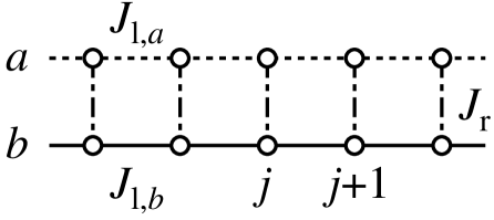
Figure 1: Sketch of the present model. Open circles denote $S\!=\!1/2$ spins, and lines three kinds of interactions between spins.

The most characteristic feature of the present system is the fact that, when the condition $J_{{\rm l},a}\!+\!J_{{\rm l},b}\!=\!0$, which belongs to the frustration region, is satisfied, the following three states are the exact eigenstates of the Hamiltonian (1).

• The direct-product singlet-dimer (SD) state in which all rungs form the SD $\bigl{(}(\alpha_{j,a}\beta_{j,b}-\beta_{j,a}\alpha_{j,b})/{\sqrt{2}}\bigr{)}$ pair.

• The direct-product triplet-dimer (TD) state in which all rungs form the TD $\bigl{(}(\alpha_{j,a}\beta_{j,b}+\beta_{j,a}\alpha_{j,b})/{\sqrt{2}}\bigr{)}$ pair.

• The nematic state with an arbitrary phase $\phi$ in which all rungs are in the state given by a linear combination of two ferromagnetic states, $\cos\phi\,\alpha_{j,a}\alpha_{j,b}\!+\!\sin\phi\,\beta_{j,a}\beta_{j,b}$.

Here, $\alpha_{j,l}$ denotes the $S_{j,l}^{z}\!=\!+1/2$ state and $\beta_{j,l}$ the $S_{j,l}^{z}\!=\!-1/2$ state. These facts can be proven by operating the Hamiltonian (1) directly to the above three states. Furthermore, it can be analytically shown that, when $J_{{\rm l},a}\!+\!J_{{\rm l},b}\!=\!0$, $J_{\rm r}\!<\!0$, and the $XY$-type anisotropy of rung interactions is sufficiently strong $\Bigl{(}$$1\!-\!\frac{2|J_{{\rm l},a}|}{|J_{\rm r}|}\!\gg\!\Delta\!\geq\!0$$\Bigr{)}$, the direct-product TD state is the exact ground state of the system, and that, when $J_{{\rm l},a}\!+\!J_{{\rm l},b}\!=\!0$ and $J_{\rm r}(>\!0)$ is sufficiently large, the direct-product SD state is the exact ground state of the system. It is noted that the above results concerning with the direct-product SD state has already been shown by Tsukano and Takahshi [12]. We also note that all of the above results including the nematic state with $\phi$ as well as the direct-product TD and SD states are applicable to systems in higher dimensions, in which units of two $S\!=\!1/2$ spins form lattices; the details will be discussed in our forthcoming paper [13].

Unfortunately, materials corresponding to the present model have been neither yet found nor synthesized so far. We believe, however, that it is a physically realistic model. In fact, for example, Yamaguchi et al. [14, 15] have recently demonstrated the modulation of magnetic interactions in spin ladder systems by using verdazyl-radical crystals. It is highly expected that the flexibility of molecular arrangements in such organic-radical materials realizes $S\!=\!1/2$ two-leg ladder systems with different leg interactions.

In the following discussions, we confine ourselves to the case where $J_{\rm r}$ is ferromagnetic, and we put $J_{\rm r}\!=\!-1$, choosing $|J_{\rm r}|$ as the unit of energy. Then, when $0\!<\!|J_{{\rm l},\ell}|\!\ll\!1$, the present ladder system can be mapped onto the $S\!=\!1$ chain by using the degenerate perturbation theory. We discuss this mapping in the next section (section 2). Section 3 is devoted to the discussions on the ground-state phase diagram. Assuming, for simplicity, that $J_{{\rm l},a}\!=-0.2$ or $0.2$ and $0\!\leq\!\Delta\!<\!1$ (the $XY$-type anisotropy of rung interactions), we determine the ground-state phase diagrams on the $\Delta$ versus $J_{{\rm l},b}$ plane. We mainly use the numerical methods such as the exact-diagonalization (ED) method and the density-matrix renormalization-group (DMRG) method [16, 17] with the help of physical considerations. Finally, we give concluding remarks in section 4.

2 Mapping onto the $S\!=\!1$ chain

We discuss the case where $0\!<\!|J_{{\rm l},\ell}|\!\ll\!|J_{\rm r}|$, assuming that $J_{\rm r}\!=\!-1$. The four eigenstates for rung $j$ are given by $\psi_{j}^{(1,+)}\!=\!\alpha_{j,a}\alpha_{j,b}$, $\psi_{j}^{(1,0)}\!=\!(\alpha_{j,a}\beta_{j,b}\!+\!\beta_{j,a}\alpha_{j,b})/{\sqrt{2}}$, $\psi_{j}^{(1,-)}\!=\!\beta_{j,a}\beta_{j,b}$ and $\psi_{j}^{(0,0)}\!=\!(\alpha_{j,a}\beta_{j,b}\!-\!\beta_{j,a}\alpha_{j,b})/{\sqrt{2}}$, and the corresponding energies are, respectively, $E^{(1,+)}\!=\!-\Delta/4$, $E^{(1,0)}\!=\!(\Delta\!-\!2)/4$, $E^{(1,-)}\!=\!-\Delta/4$ and $E^{(0,0)}\!=\!(\Delta\!+\!2)/4$, for all $j$’s. Thus, the state $\psi_{j}^{(0,0)}$ can be neglected. We introduce the pseudo $S\!=\!1$ operator ${\vec{T}}_{j}$ for rung $j$, and make the $T_{j}^{z}\!=\!+1$, $0$ and $-1$ states correspond to the $\psi_{j}^{(1,+)}$, $\psi_{j}^{(1,0)}$ and $\psi_{j}^{(1,-)}$ states, respectively. The relation ${\vec{T}}_{j}\!=\!{\vec{S}}_{j,a}\!+\!{\vec{S}}_{j,b}$ holds, as is readily shown by comparing the matrix elements of both operators ${\vec{T}}_{j}$ and ${\vec{S}}_{j,l}$ in the subspace of $\phi_{j}^{(1,+)}$, $\phi_{j}^{(1,0)}$ and $\phi_{j}^{(1,-)}$. Thus, the Hamiltonian (1) for the $S\!=\!1/2$ operator ${\vec{S}}_{j,l}$ can be mapped onto the effective Hamiltonian ${\cal H}_{{\rm eff}}$ for the $S\!=\!1$ operator ${\vec{T}}_{j}$, which is given by

$${\cal H}_{{\rm eff}}=J_{\rm eff}\sum_{j=1}^{L}{\vec{T}}_{j}\cdot{\vec{T}}_{j+1}+D_{\rm eff}\sum_{j=1}^{L}(T_{j}^{z})^{2}\,;\quad J_{\rm eff}=\frac{J_{{\rm l},a}+J_{{\rm l},b}}{4}\,,\quad D_{\rm eff}=\frac{(1-\Delta)}{2},$$ (2)

where $T_{j}^{z}$ is the $z$-component of ${\vec{T}}_{j}$. It is noted that the on-site anisotropy ($D_{\rm eff}$-) term comes from the difference between $E^{(1,+)}=E^{(1,-)}$ and $E^{(1,0)}$.

The above ${\cal H}_{{\rm eff}}$ is the result of the degenerate perturbation calculation in the lowest-order of $|J_{{\rm l},\ell}|/|J_{\rm r}|$. It is apparent that this is not applicable to discussing the frustrated region of the original Hamiltonian (1), which includes the case of $J_{{\rm l},a}\!+\!J_{{\rm l},b}\!=\!0$. In order to improve this point, higher-order perturbation calculations are indispensable; these calculations are left for a future study.

The ground-state phase diagram of the anisotropic $S\!=\!1$ chain has been determined by several authors [18, 19, 20]. According to their results, as the value of $D_{\rm eff}$ increases from zero, the phase transition from the $XY$ (or Haldane) phase to the large-$D$ phase takes place at $D_{\rm eff}\!\simeq\!1$ when $J_{\rm eff}\!=-1$ (or when $J_{\rm eff}\!=1$). Thus, we may expect that in our $S\!=\!1/2$ ladder with $J_{\rm r}\!=\!-1$, the phase transition between the $XY$ and TD phases occurs at $J_{{\rm l},a}\!+\!J_{{\rm l},b}\!\simeq\!2(\Delta\!-\!1)$ when $J_{{\rm l},a}\!+\!J_{{\rm l},b}\!<\!0$ (or, equivalently, when $\Delta\!<\!1$), and also that the phase transition between the Haldane and TD phases occurs at $J_{{\rm l},a}\!+\!J_{{\rm l},b}\!\simeq\!2(1\!-\!\Delta\!)$ when $J_{{\rm l},a}\!+\!J_{{\rm l},b}\!>\!0$ (or, when $\Delta\!<\!1$, again). It is noted that the large-$D$ state in the spin-1 chain is equivalent to the TD state in the present $S\!=\!1/2$ ladder, since in the valence bond picture of the former state, each $S\!=\!1$ spin consists of two $S\!=\!1/2$ spins forming the TD pair, as is well known.

3 Ground-state phase diagrams

Throughout this section we assume that $J_{{\rm r}}\!=\!-1$, as mentioned before. Figure 2 shows the ground-state phase diagrams on the $\Delta$ versus $J_{{\rm l},b}$ plane determined for $J_{{\rm l},a}\!=\!-0.2$ and $J_{{\rm l}.a}\!=\!0.2$. The former phase diagram consists of the TD, $XY$ and non-collinear ferrimagnetic (NCFR) phases [12, 21], and in the latter one, the Haldane (H) phase appears in addition to the above three phases. There are three kinds of the phase transition lines, which we have numerically estimated as discussed below in detail. The magenta lines with open circles are the phase transition lines between the TD or H phase and the $XY$ phase which are of the Berezinskii-Kosterlitz-Thouless (BKT) type [22, 23], the red line with closed circles is the phase transition line between the TD and H phases which are of the Gaussian-type, and finally the blue lines with open squares are the phase transition lines between the NCFR phase and the TD or $XY$ phase. In the latter phase diagram, there are two tricritical points at $(\Delta,J_{{\rm l},b})\!=\!\bigl{(}0.500(1),1.917(1)\bigr{)}$ and $\bigl{(}0.945(1),-0.052(1)\bigr{)}$ associated with TD, $XY$ and H phases. The green straight lines show the results of the comparison of the degenerate perturbation calculations with the numerical results [18, 19, 20] (see section 2); in Fig. 2(a) it is for the TD-$XY$ transition and given by $J_{{\rm l},b}\!=\!2\Delta\!-\!1.8$, while in Fig. 2(b) it is for the TD-H transition and given by $J_{{\rm l},b}\!=\!-2\Delta\!+\!1.8$. In both cases they are in excellent agreement with the numerical results at least when $|J_{{\rm l},b}|$ is not too large. It is noted that on the special lines where $J_{{\rm l},a}\!+\!J_{{\rm l},b}\!=\!0$, which are shown by the black broken lines, the direct-product TD state is the exact ground state.

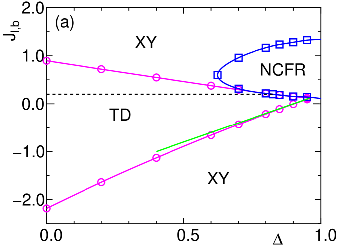
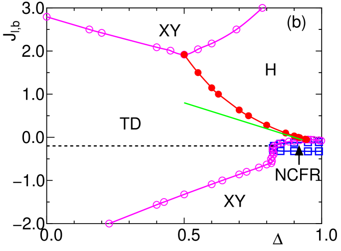
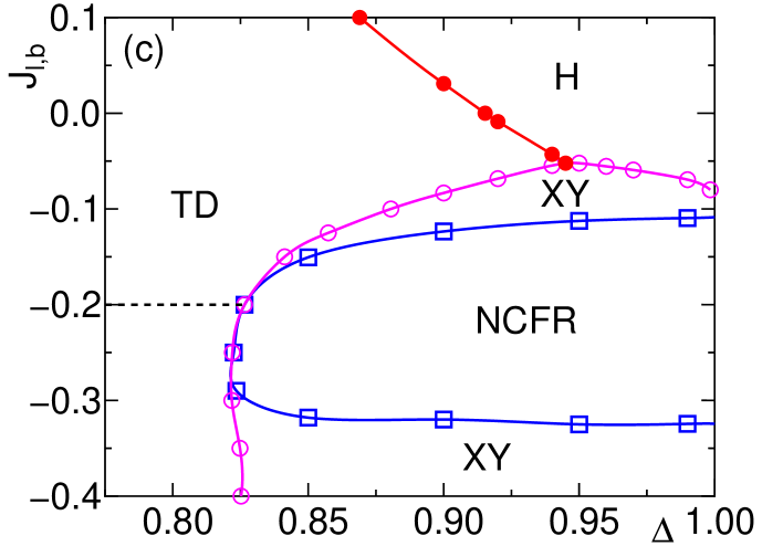
Figure 2: Ground-state phase diagram on the $\Delta$ versus $J_{{\rm l},b}$ plane for (a) $J_{{\rm l},a}\!=\!-0.2$ and (b,c) $J_{{\rm l},a}\!=\!0.2$ with $J_{{\rm r}}\!=\!-1$; in (c) part of (b) is enlarged. The regions designated by TD, XY, NCFR and H are, respectively, those of the triplet-dimer, $XY$, non-collinear ferrimagnetic and Haldane phases. See the text for the meanings of several lines.

In the following explanations for the estimation of the above phase boundary lines, we denote, respectively, by $E_{0}(L,M;{\rm pbc})$ and $E_{1}(L,M;{\rm pbc})$ the lowest and second-lowest energy eigenvalues of the Hamiltonian (1) within the subspace determined by $L$ and $M$ under periodic boundary conditions, ${\vec{S}}_{L+1,\ell}\!=\!{\vec{S}}_{1,\ell}$. The quantity $M$ is the total magnetization given by $M\!=\!\sum_{j=1}^{L}(S_{j,a}^{z}\!+\!S_{j,b}^{z})$, which is a good quantum number with the eigenvalues of $M\!=\!0$, $\pm 1$, $\cdots$, $\pm L$. Similarly, we also denote by $E_{0}(L,M,P;{\rm tbc})$ the lowest energy eigenvalue of the Hamiltonian (1) within the subspace determined by $L$, $M$ and $P$ under twisted boundary conditions, $S_{L+1,\ell}^{x}\!=\!-S_{1,\ell}^{x}$, $S_{L+1,\ell}^{y}\!=\!-S_{1,\ell}^{y}$ and $S_{L+1,\ell}^{z}\!=\!S_{1,\ell}^{z}$, where $P(=\!+1$ or $-1)$ is the eigenvalue of the space inversion operator with respect to the twisted bond, ${\vec{S}}_{j,\ell}\!\leftrightarrow\!{\vec{S}}_{L+1-j,\ell}$. We further denote by $E_{0}(L,M;{\rm obc})$ the lowest energy eigenvalue of the Hamiltonian (1) within the subspace determined by $L$ and $M$ under open boundary conditions, where the sums over $j$ for leg interactions are taken from $j\!=\!1$ to $L\!-\!1$.

The most powerful method to estimate numerically the phase boundary lines between two of the TD, $XY$ and H phases is the level spectroscopy (LS) method developed by Okamoto, Nomura and Kitazawa [24, 25, 26, 27]. In this method, the following three excitation energies [28], $\Delta E_{02}^{({\rm p})}(L)\!=\!E_{0}(L,2;{\rm pbc})\!-\!E_{0}(L,0;{\rm pbc})$, $\Delta E_{00}^{({\rm p},{\rm t})}(L,+1)\!=\!E_{0}(L,0,+1;{\rm tbc})\!-\!E_{0}(L,0;{\rm pbc})$ and $\Delta E_{00}^{({\rm p},{\rm t})}(L,-1)\!=\!E_{0}(L,0,-1;{\rm tbc})\!-\!E_{0}(L,0;{\rm pbc})$ should be compared in the thermodynamic ($L\!\to\!\infty$) limit. More strictly speaking, the critical value $J_{{\rm l},b\,({\rm cr})}^{(XY,{\rm TD})}$ of the BKT $XY$-TD transition, the critical value $J_{{\rm l},b\,({\rm cr})}^{(XY,{\rm H})}$ of the BKT $XY$-H transition and the critical value $J_{{\rm l},b\,({\rm cr})}^{({\rm TD,H})}$ of the Gaussian TD-H transition, which are all for given values of $J_{{\rm l},a}$ and $\Delta$, are estimated as follows. First, the corresponding finite-size critical values $J_{{\rm l},b\,({\rm cr})}^{(XY,{\rm TD})}(L)$, $J_{{\rm l},b\,({\rm cr})}^{(XY,{\rm H})}(L)$ and $J_{{\rm l},b\,({\rm cr})}^{({\rm TD,H})}(L)$ are estimated, respectively, by solving numerically the equations [29],

$$\Delta E_{02}^{({\rm p})}(L)=\Delta E_{00}^{({\rm p},{\rm t})}(L,+1)<\Delta E_{00}^{({\rm p},{\rm t})}(L,-1)\,,$$ (3)

$$\Delta E_{02}^{({\rm p})}(L)=\Delta E_{00}^{({\rm p},{\rm t})}(L,-1)<\Delta E_{00}^{({\rm p},{\rm t})}(L,+1)\,,$$ (4)

$$\Delta E_{00}^{({\rm p},{\rm t})}(L,+1)=\Delta E_{00}^{({\rm p},{\rm t})}(L,-1)<\Delta E_{02}^{({\rm p})}(L)\,.$$ (5)

Then, these finite-size results are extrapolated to the $L\!\to\!\infty$ limit to obtain, respectively, the critical values, $J_{{\rm l},b\,({\rm cr})}^{(XY,{\rm TD})}$, $J_{{\rm l},b\,({\rm cr})}^{(XY,{\rm H})}$ and $J_{{\rm l},b\,({\rm cr})}^{({\rm TD,H})}$.

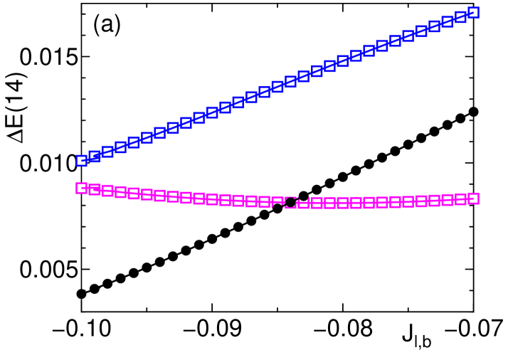
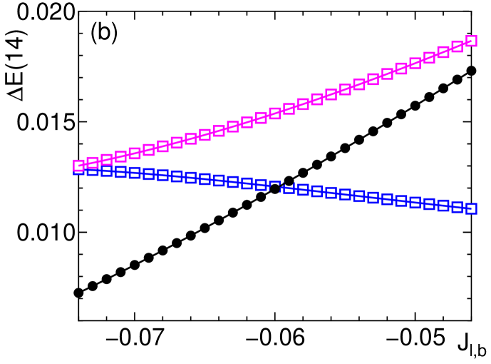
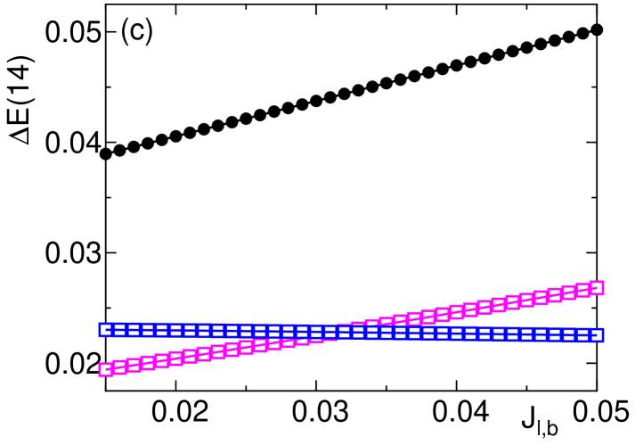
Figure 3: Examples of the $\Delta E_{02}^{({\rm p})}(14)$ (black closed circles), $\Delta E_{00}^{({\rm p},{\rm t})}(14,+1)$ (magenta open squares) and $\Delta E_{00}^{({\rm p},{\rm t})}(14,-1)$ (blue open squares) versus $J_{{\rm l},b}$ curves for (a,c) $\Delta\!=\!0.90$ and (b) $\Delta\!=\!0.97$ with $J_{{\rm l},a}\!=\!0.2$ and $J_{\rm r}\!=\!-1$ $\bigl{(}$see Fig. 2(c).$\bigr{)}$ In (a), (b) and (c) we obtain, respectively, $J_{{\rm l},b\,({\rm cr})}^{(XY,{\rm TD})}(14)\!=\!-0.084049$ from the crossing point of the black and magenta curves, $J_{{\rm l},b\,({\rm cr})}^{(XY,{\rm H})}(14)\!=\!-0.059748$ from the crossing point of the black and blue curves and $J_{{\rm l},b\,({\rm cr})}^{({\rm TD,H})}(14)\!=\!0.031604$ from the crossing point of the magenta and blue curves.

Figure 4: Examples of the $L\!\to\!\infty$ extrapolations of (a) $J_{{\rm l},b\,({\rm cr})}^{(XY,{\rm TD})}(L)$ for $\Delta\!=\!0.90$, (b) $J_{{\rm l},b\,({\rm cr})}^{(XY,{\rm H})}(L)$ for $\Delta\!=\!0.97$ and (c) $J_{{\rm l},b\,({\rm cr})}^{({\rm TD,H})}(L)$ for $\Delta\!=\!0.90$, where $J_{{\rm l},a}\!=\!0.2$ and $J_{\rm r}\!=\!-1$ $\bigl{(}$see Fig. 2(c).$\big{)}$ We assume that these finite-size critical values are quadratic functions of $1/L^{2}$. The broken lines represent the least-square fittings by use of $L\!=\!14$, $12$, $10$ and $8$ data, while the solid lines those without $L\!=\!8$ data. From these extrapolations, we obtain $J_{{\rm l},b\,({\rm cr})}^{(XY,{\rm TD})}\!=\!-0.0833(1)$ in (a), $J_{{\rm l},b\,({\rm cr})}^{(XY,{\rm H})}\!=\!-0.0593(1)$ in (b) and $J_{{\rm l},b\,({\rm cr})}^{({\rm TD,H})}\!=\!0.0309(1)$ in (c), where the numerical errors are estimated from the difference between the extrapolated results with and without the $L\!=\!8$ data.

Practically, we have made the ED calculations to estimate $J_{{\rm l},b\,({\rm cr})}^{(XY,{\rm TD})}(L)$, $J_{{\rm l},b\,({\rm cr})}^{(XY,{\rm H})}(L)$ and $J_{{\rm l},b\,({\rm cr})}^{({\rm TD,H})}(L)$ for finite-$L$ systems with $2L\!=\!12$, $16$, $\cdots$, $28$ spins. The procedures for these estimations are shown in Fig. 3, for example, for $L\!=\!14$, $J_{{\rm l},a}\!=\!0.2$ and $\Delta\!=\!0.90$ or $0.97$. Performing the $L\!\to\!\infty$ extrapolations of the above finite-size critical values, we have fitted them to quadratic functions of $1/L^{2}$ by use of the least-square method, as explained in Fig. 4, for example, for $J_{{\rm l},a}\!=\!0.2$ and $\Delta\!=\!0.90$ or $0.97$, again. Then, as the results of the extrapolations, we have obtained in the $J_{{\rm l},a}\!=\!0.2$ case, $J_{{\rm l},b\,({\rm cr})}^{(XY,{\rm TD})}\!=\!-0.0833(1)$ and $J_{{\rm l},b\,({\rm cr})}^{({\rm TD,H})}\!=\!0.0309(1)$ for $\Delta\!=\!0.90$, and also $J_{{\rm l},b\,({\rm cr})}^{(XY,{\rm H})}\!=\!-0.0593(1)$ for $\Delta\!=\!0.97$. The phase transition lines shown by the magenta and red lines in Fig. 2(b) and (c) are drawn by plotting, as functions of $\Delta$, the values of $J_{{\rm l},b\,({\rm cr})}^{(XY,{\rm TD})}$, $J_{{\rm l},b\,({\rm cr})}^{({\rm TD,H})}$, and $J_{{\rm l},b\,({\rm cr})}^{(XY,{\rm H})}$ calculated for various values of $\Delta$. Similarly, the phase transition lines shown by the magenta lines in Fig. 2(a) are obtained by calculating $J_{{\rm l},b\,({\rm cr})}^{(XY,{\rm TD})}$ and $J_{{\rm l},b\,({\rm cr})}^{({\rm TD,H})}$ for various values of $\Delta$ in the case of $J_{{\rm l},a}\!=\!-0.2$.

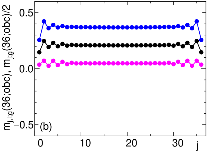
Figure 5: (a) Plot of $m_{\rm g}(36;{\rm obc})$ versus $J_{{\rm l},b}$, (b) those of $m_{j;{\rm g}}(36;{\rm obc})/2$ (black line), $m_{j,a;{\rm g}}(36;{\rm obc})$ (blue line) and $m_{j,b;{\rm g}}(36;{\rm obc})$ (magenta line) versus $j$ and (c) that of $|S_{q;{\rm g}}(36;{\rm obc})|^{2}$ versus $q/\pi$. The quantity $m_{\rm g}(36;{\rm obc})$ in (a) is obtained in the case where $J_{{\rm l},a}\!=\!-0.2$, $\Delta\!=\!0.8$ and $J_{\rm r}\!=\!-1$, while those $m_{j;{\rm g}}(36;{\rm obc})$ and $|S_{q;{\rm g}}(36;{\rm obc})|^{2}$ in (b,c) are obtained in the case where $J_{{\rm l},a}\!=\!-0.2$, $J_{{\rm l},b}\!=\!0.7$, $\Delta\!=\!0.8$ and $J_{\rm r}\!=\!-1$. $\bigl{(}$see Fig. 2(a).$\big{)}$

Let us denote by $M_{\rm g}(L;{\rm obc})$ the ground-state magnetization for the system with $2L$ spins under open boundary conditions, which is the value of $M$ giving the lowest value of $E_{0}(L,M;{\rm obc})$’s. In the NCFR phase, $M_{\rm g}(L;{\rm obc})$ is finite $\bigl{(}$$0\!<\!M_{\rm g}(L;{\rm obc})\!<\!L$$\bigr{)}$, while in other phases, $M_{\rm g}(L;{\rm obc})\!=\!0$ [28]. We have carried out DMRG calculations [16, 17] for the finite system with $2L\!=\!72$ spins to estimate the ground-state magnetization per spin, $m_{\rm g}(L;{\rm obc})$, which is defined by $m_{\rm g}(L;{\rm obc})\!=\!M_{\rm g}(L;{\rm obc})/(2L)$. The obtained results in the case where $J_{{\rm l},a}\!=\!-0.2$ and $\Delta\!=\!0.8$ are depicted in Fig. 5(a). We see from this figure that the phase transition from the TD phase to the NCFR phase and that from the NCFR phase to the $XY$ phase successively occur with increasing $J_{{\rm l},b}$ $\bigl{(}$see Fig. 2(a)$\bigr{)}$. The finite-size critical values for the former and latter transitions in the $J_{{\rm l},a}\!=\!-0.2$ and $\Delta\!=\!0.8$ case are given, respectively, by $J_{{\rm l},b\,({\rm cr})}^{({\rm TD},{\rm NCFR})}(36)\!=\!0.2185(5)$ and $J_{{\rm l},b\,({\rm cr})}^{({\rm NCFR},XY)}(36)\!=\!1.1675(5)$. We have performed these DMRG calculations for various $\Delta$’s with $J_{{\rm l},a}$ fixed at $J_{{\rm l},a}\!=\!-0.2$, and obtained the phase transition line shown by the blue line in Fig. 2(a), supposing that the results in the $L\!=\!36$ system give good approximate results in the $L\!\to\!\infty$ limit [30]. Similarly, the phase transition line shown by the blue line in Fig. 2(b,c) has been obtained by means of the DMRG calculations in the case of $J_{{\rm l},a}\!=\!0.2$.

Figure 5(a) suggests that the phase transition between the TD and NCFR phases is of the second order, while that between the NCFR and $XY$ phases is of the first order. However, it is fairly difficult to clarify the order of the phase transition by using only the results of DMRG calculations.

We have also calculated the ground-state site magnetization $m_{j,\ell;{\rm g}}(L;{\rm obc})$ by use of the DMRG method [16, 17]. This quantity is defined by $m_{j,\ell;{\rm g}}(L;{\rm obc})\!=\!\langle S_{j,\ell}^{z}\rangle_{L;{\rm g}}$, where $\langle\cdots\rangle_{L;{\rm g}}$ denotes the expectation value with respect to the ground state of the Hamiltonian (1) under open boundary conditions. Of course, the relation $\sum_{j=1}^{L}\big{\{}m_{j,a;{\rm g}}(L;{\rm obc})\!+\!m_{j,b;{\rm g}}(L;{\rm obc})\bigr{\}}\!=\!M_{\rm g}(L;{\rm obc})$ holds. In Fig. 5(b) we plot the $j$-dependences of the ground-state rung magnetization $m_{j;{\rm g}}(L;{\rm obc})\bigl{(}=\!m_{j,a;{\rm g}}(L;{\rm obc})\!+\!m_{j,b;{\rm g}}(L;{\rm obc})\bigr{)}$ and $m_{j,\ell;{\rm g}}(L;{\rm obc})$, calculated for the $L\!=\!36$ system in the case where $J_{{\rm l},a}\!=\!-0.2$, $J_{{\rm l},b}\!=\!0.7$ and $\Delta\!=\!0.8$; for these parameters $M_{\rm g}(L;{\rm obc})\!=\!15$. This figure demonstrates that the $j$-dependences of these quantities are not uniform especially near both of open boundaries. Paying attention to this fact, we have examined the Fourier transform $S_{q;{\rm g}}(L;{\rm obc})$ of $m_{j;{\rm g}}(L;{\rm obc})$ [31, 32], defined by

$$S_{q;{\rm g}}(L;{\rm obc})=\frac{1}{\sqrt{L}}\sum_{j=1}^{L}\exp(iqj)\,\biggl{\{}m_{j;{\rm g}}(L;{\rm obc})-\frac{M_{\rm g}(L;{\rm obc})}{2L}\biggr{\}}\,,$$ (6)

where $q$ is the wave number. The squared modulus $|S_{q;{\rm g}}(L;{\rm obc})|^{2}$ of this quantity, calculated for the $L\!=\!36$ system in the $J_{{\rm l},a}\!=\!-0.2$, $J_{{\rm l},b}\!=\!0.7$ and $\Delta\!=\!0.8$ case, where $M_{\rm g}(L;{\rm obc})\!=\!15$, is plotted as a function of $q/\pi$ in Fig. 5(c). This figure shows that the largest peak of $|S_{q;{\rm g}}(36;{\rm obc})|^{2}$ appears at the position closest to $q=\pi$, suggesting that the wave number of the dominant excitation in the NCFR state is $q=\pi$. $\bigl{(}$Note that in the system with even $L$ under open boundary conditions, $|S_{q;{\rm g}}(L;{\rm obc})|^{2}$ at $q=\pi$ is exactly zero because of the space-inversion symmetry $m_{j;{\rm g}}(L;{\rm obc})=m_{L+1-j;{\rm g}}(L;{\rm obc})$.$\bigr{)}$ We therefore expect that the NCFR state has a commensurate character. In order to examine the commensurability of the NCFR state in full detail, it is necessary to treat the Fourier transform of the rung magnetization $m_{j;{\rm g}}(L;{\rm obc})$ as well as that of the ground-state two-spin correlation function $\langle S_{j,\ell}^{z}\,S_{j^{\prime},\ell}^{z}\rangle_{L;{\rm g}}$ in larger systems. We will discuss this problem in the near future.

4 Concluding remarks

We have numerically determined, with the help of some physical considerations, the ground-state phase diagrams of the $S\!=\!1/2$ two-leg ladder with different leg interactions, which is governed by the Hamiltonian (1), in the cases where $J_{{\rm l},a}\!=\pm\,0.2$, $J_{\rm r}\!=\!-1$ and $0\!\leq\!\Delta\!<\!1$. The obtained phase diagrams on the $\Delta$ versus $J_{{\rm l},b}$ plane are shown in Fig. 2. The characteristic features of the results are as follows:

• The NCFR state appears as the ground state in the region where $J_{{\rm l},a}J_{{\rm l},b}\!<\!0$, when $\Delta$ is not too small.

• The direct-product TD state is the exact ground state, when $J_{{\rm l},a}\!+\!J_{{\rm l},b}\!=\!0$ and $0\!\leq\!\Delta\,$$<$$\sim$$\,0.83$.

It is emphasized that these results are attributed to the frustration effect.

We hope that the present research stimulates future experimental studies on related subjects, which include the synthesization of spin ladder systems with different leg interactions.

We would like to express our sincere thanks to Professors K Hida and H Yamaguchi for their invaluable discussions and comments. This work has been partly supported by JSPS KAKENHI Grant Numbers 15K05198, 16K05419 and 15K05882 (J-Physics) and also by Hyogo Science and Technology Association. Finally, we thank the Supercomputer Center, Institute for Solid State Physics, University of Tokyo and the Computer Room, Yukawa Institute for Theoretical Physics, Kyoto University for computational facilities.

References

References

- [1] Lavarélo A, Guillaume G and Laflorencie N 2011 \PRB 84 144407 and references therein
- [2] Vekua T and Honecker A 2006 \PRB 73 214427 and references therein
- [3] Michaud F, Coletta T, Manmana S R, Picon J-D and Mila F 2010 \PRB 81 014407 and references therein
- [4] Tonegawa T, Okamoto K, Hikihara T and Sakai T 2016 J. Phys.: Conf. Series 683 012039
- [5] Okamoto K and Ichikawa Y 2002 J. Phys. Chem. Solids 63 1575
- [6] Okamoto K 2002 Prog. Theor. Phys. Suppl. No.145 208
- [7] Tokuno A and Okamoto K 2005 J. Phys. Soc. Jpn. 74 Suppl. 157
- [8] Okamoto K 2014 JPS Conf. Proc. 1 012031
- [9] Amiri F, Sun G, Mikeska H-J and Vekua T 2015 \PRB 92 184421
- [10] Japaridze G I and Pogosyan E 2006 \JPCM18 9297
- [11] Oshikawa M, Yamanaka M and Affleck I 1997 \PRL78 1984
- [12] Tsukano M and Takahashi M 1997 J. Phys. Soc. Jpn. 66 1153
- [13] Hikihara T, Tonegawa T, Okamoto K and Sakai T in preparation
- [14] Yamaguchi H, Iwase K, Ono T, Shimokawa T, Nakano H, Shimura Y, Kase N, Kittaka S, Sakakibara T, Kawakami T, and Hosokoshi Y 2013 \PRL110 157205
- [15] Yamaguchi H, Miyagai H, Shimokawa T, Iwase K, Ono T, Kono Y, Kase N, Araki K, Kittaka S, Sakakibara T, Kawakami T, Okunishi K and Hosokoshi Y 2014 J. Phys. Soc. Jpn. 83 033707
- [16] White S R 1992 \PRL69 2863
- [17] White S R 1993 \PRB 48 10345
- [18] Chen W, Hida K and Sanctuary B C 2003 \PRB 67 104401
- [19] Hu S, Normand B, Wang X and Yu L 2011 \PRB 84 220402(R)
- [20] Wierschem K and Sengupta P 2014 \PRB 90 115157
- [21] Yoshikawa S and Miyashita S 2005 J. Phys. Soc. Jpn. Suppl. 74 71
- [22] Berezinskii Z L 1971 Sov. Phys. JETP 34 610
- [23] Kosterlitz J M and Thouless D J 1973 J. Phys. C 6 1181
- [24] Okamoto K and Nomura K 1992 \PLA 169 433
- [25] Nomura K and Okamoto K 1994 J. Phys. A 27 5773
- [26] Kitazawa A 1997 J. Phys. A 30 L285
- [27] Nomura K and Kitazawa A 1998 J. Phys. 31 7341
- [28] We note that in the TD, and H phase regions, always gives the ground-state energy of the finite- system under periodic boundary conditions.
- [29] Here, to solve the equation means that to solve the equation under the conditions and (see Fig. 3).
- [30] We have made sure that, for a few values of and , the results in the system are not so much different from those in the system.
- [31] Hikihara T, Kecke L, Momoi T and Furusaki A 2008 \PRB 78 144404
- [32] Hikihara T, Momoi T, Furusaki A and Kawamura H 2010 \PRB 81 224433