A numerical solution of one class of Volterra integral equations of the first kind in terms of the machine arithmetic features

Abstract

The research is devoted to a numerical solution of the Volterra equations of the first kind that were obtained using the Laplace integral transforms for solving the equation of heat conduction. The paper consists of an introduction and two sections. The first section deals with the calculation of kernels from the respective integral equations at a fixed length of the significand in the floating point representation of a real number. The PASCAL language was used to develop the software for the calculation of kernels, which implements the function of tracking the valid digits of the significand. The test examples illustrate the typical cases of systematic error accumulation. The second section presents the results obtained from the computational algorithms which are based on the product integration method and the midpoint rule. The results of test calculations are presented to demonstrate the performance of the difference methods.

Introduction

The paper is devoted to the studies on a special class of Volterra integral equations of the first kind

$$\int\limits_{0}^{t}K_{N}(t-s)\phi(s)ds={y}(t),\,\,$$ (1)

$$K_{N}(t-s)=\sum\limits_{q=1}^{N}{\left({-1}\right)^{q+1}q^{2}e^{-\pi^{2}q^{2}\left({t-s}\right)}}.$$ (2)

The specific feature of kernel $K_{N}(t-s)$ in (2) lies in that $K_{N}=0$ in some neighborhood of zero. The qualitative theory and numerical methods of solving the Volterra equations of the first kind are dealt with in many studies (for example, [1, 2, 3, 4] and the eqreferences given in them).

The goal of this paper is to consider the application of numerical methods for solving the equations of form (1), (2) taking into account the mechanisms of error occurrence in the computer calculations. The work is a continuation of the research started in [5, 6].

The Volterra equation of the convolution type (1), (2) was first obtained in [7]. The authors of [7] suggest a method of searching for a solution $u(1,t)=\phi(t)$, $t\geq 0$, of an inverse boundary-value problem

$$u_{t}=u_{xx},\quad x\in\left({0,1}\right),\quad t\geqslant 0,$$ (3)

$$u\left({x,0}\right)=0,\;u\left({0,t}\right)=0,\;u_{x}\left({0,t}\right)=g_{0}\left({t}\right)\;$$ (4)

by reducing (3), (4) to the Volterra integral equation of convolution type:

$$\int\limits_{0}^{t}K(t-s)\phi(s)ds={y}(t),\,\,0\leq s\leq t\leq T,$$ (5)

$$K(t-s)=\sum\limits_{q=1}^{\infty}{\left({-1}\right)^{q+1}q^{2}e^{-\pi^{2}q^{2}\left({t-s}\right)}},\;{y}(t)=\frac{1}{2\pi^{2}}g_{0}\left({t}\right).$$ (6)

Instead of $g_{0}(t)$ we normally know $g_{\delta}(t)$: ${\left\|{g_{\delta}(t)-g_{0}}(t)\right\|}_{C}\leqslant\delta$, $\delta>0.$

Problem (3), (4) plays an important part in the applied problems, including those related to the research into non-stationary thermal processes. Solving the inverse problems is as a rule complicated by the instability of these problems with respect to the initial data errors. The application of the methods which employ the Fourier and Laplace transforms in combination with the theory of ill-posed problems found wide application in the construction of stable solutions to the inverse problems of heat conductance. In particular, to solve the problem similar to (3), (4), the authors of [8] used a stabilizing functional after applying the Fourier transform. In [9] to regularize and assess the convergence of the obtained solutions the authors used a method of conjugate gradients. In [10] and [11] the Laplace transform was considered for solving the Cauchy problem. In [12] the Laplace transform was used in a two-dimensional problem. The existing approaches, as a rule, after taking the Laplace transform, apply regularization methods to the obtained equations and then perform the inverse transform.

Taking into account the ideas from [13, 14] the authors of [7] approximated $u_{x}(0,t)$ by the sum $N$ of the first summands:

$$u_{x}(0,t)=2\pi^{2}\sum\limits_{q=1}^{N}{\left({-1}\right)^{q+1}q^{2}\int\limits_{0}^{t}e^{-\pi^{2}q^{2}\left({t-s}\right)}}\phi(s)ds,$$

where $N$ is positive integer. Then (5), (6) are reduced to the form (1), (2). The performance of this approach was discussed in [7]. According to the conclusion made by the author, such a way of solving the inverse problem makes it possible to reduce the initial problem to the Volterra integral equation of the first kind and exclude the components of the operator calculus from the regularization process.

It is known that the Volterra integral equations of the first kind belong to the class of conditionally-correct problems, and the discretization procedure has a regularizing feature with a regularization parameter, a step of mesh, which is in a certain manner connected to the level of disturbances of the initial data $\delta$.

This paper presents an algorithm to numerically solve (1), (2) at an exactly specified right-hand part. Note that when solving (1), (2) we face three types of errors related first of all to the approximation of the initial problem (5), (6), secondly to the accuracy of a numerical method, and finally to the computation errors in the machine arithmetic operations with real floating-point numbers. For the research, of greatest interest is the first of the indicated cases. However, to pass to the problem of assessing the parameter $N$ in (2) it is necessary to develop an algorithm for computation of $K_{N_{\max}}$, which takes into account the specific features of machine arithmetic and provides the desired (specified) number of valid digits in the significand.

1 The specific features of the numerical
calculations

The computational experiment in [5] shows that with an increase in the number of summands in (2) the roots $\lambda^{*}$ of the equation $K_{N}(\lambda)=0$ decrease (at the same time monotonisity is observed only separately in even and odd $N$). The values $\lambda^{*}$ will be used further to limit the magnitude of the mesh step $h$ from above, for the value of the mesh function $K^{h}_{N}$ at the first node to be non-zero. As is known, the condition $K_{N}(0)\neq 0$ is necessary for (1), (2) to be correct on the pair $(C,C^{1}_{[0,T]})$, where $y(0)=0$, $y^{\prime}(t)\in C_{[0,T]}$.

Note, that there can be computational errors in the calculation of $\lambda^{*}$, they can be related to the application of a fixed mesh in the machine number representation.

Let us consider the known cases of systematic error accumulation [15] which appear in the calculation of kernel values (2). Use the system of computer algebra Maple10. Following [16] we will include parameter $f$ in the generally accepted representation of the real number. The parameter is equal to the number of valid digits in the significand (starting from the left). Assume that the real number $x=s\cdot M\cdot 10^{-L+p}$ is specified by the set $(s,M,p,f)$, where $s\in\{-1,0,+1\}$ is the sign of the number, $M\in\{10^{L-1},10^{L-1}+1,...,10^{L}-1\}\cup\{0\}$ is significand of the number, $L$ is number of significand positions, $p$ is exponent part of the number.

Let us illustrate the details of the calculations when summing up the numbers with different exponent parts in (2), using the example.

Example 1. Let $N=50$, $\lambda_{0}=10^{-3}$, $L\geq 8$. Take

$$x_{1}=\sum\limits_{q=11}^{34}{\left({-1}\right)^{q+1}q^{2}e^{-\pi^{2}q^{2}{\lambda_{0}}}},\;x_{2}=\sum\limits_{q=35}^{50}{\left({-1}\right)^{q+1}q^{2}e^{-\pi^{2}q^{2}{\lambda_{0}}}}$$

and find $x_{\Sigma}=x_{1}+x_{2}$.

Assuming

$$10^{p_{\Sigma}-f_{\Sigma}}=10^{p_{1}-f_{1}}+10^{p_{2}-f_{2}},\;p_{\Sigma}\geq p_{1}\geq p_{2},$$

according to [16], it is easy to obtain that

$$f_{\Sigma}\geq f_{s}=[f_{1}-\lg(1+10^{-p_{1}+f_{1}+p_{2}-f_{2}})],$$ (7)

where the symbol $[...]$ means the greatest integer. The last column of the table shows the values of minorant $f_{s}$, that are calculated using (7). Tab. 1 presents the parameters $(1,M_{1},2,f_{1})$, $(1,M_{2},-2,f_{2})$ and $(1,M_{\Sigma},2,f_{\Sigma})$, which define $x_{1}$, $x_{2}$ and $x_{\Sigma}$ respectively.

Table 1

Values $M$ and $f$ for $x_{1}$, $x_{2}$ and $x_{\Sigma}$.

$L$	$M_{1}$	$f_{1}$	$M_{2}$	$f_{2}$	$M_{\Sigma}$	$f_{\Sigma}$	$f_{s}$
8	18652239	6	44981421	6	18656737	6	5
9	186522441	8	449814458	7	186567422	8	7
10	1865224455	9	4498144699	8	1865674269	8	8
11	18652244592	11	44981446726	8	18656742737	11	10
12	186522445926	11	449814466957	10	186567427373	11	10
13	1865224459248	12	4498144669376	10	1865674273715	12	11
14	18652244592468	13	44981446694089	11	18656742737137	13	12

The next example illustrates the situation arising in the calculation of the difference between the numbers which have coinciding exponent parts and several high-order digits of the significand.

Example 2. Let $N=50$, $\lambda_{0}=10^{-3}$, $L\geq 8$. Introduce

$$x_{3}=\sum\limits_{q=1}^{10}{\left({-1}\right)^{q+1}q^{2}e^{-\pi^{2}q^{2}{\lambda_{0}}}},\;\;x_{4}=\sum\limits_{q=11}^{50}{\left({-1}\right)^{q+1}q^{2}e^{-\pi^{2}q^{2}{\lambda_{0}}}}.$$

Define $x_{\Delta}=|x_{4}|-|x_{3}|$. Suppose that

$$|M_{4}-M_{3}|<10^{L-1}-1,\;p_{\Delta}\leq p_{3}=p_{4}$$

and, following [16] use the empiric estimate:

$$f_{\Delta}\geq f_{r}=\left\{{\begin{array}[]{l}{\;0,\;\text{if}\;\,f_{\min}-L+\lg(\lambda)\leq 0,}\\ {\left[f_{\min}-L+\lg(\lambda)\right],\;\text{if}\;\,f_{\min}-L+\lg(\lambda)>0},\end{array}}\ \right.$$ (8)

where $\lambda=|M_{4}-M_{3}|+1,$ $f_{\min}=\min\{f_{3},\,f_{4}\}$.

Below are the parameters $(-1,M_{3},2,f_{3})$, $(1,M_{4},2,f_{4})$ and $(-1,M_{\Delta},2,f_{\Delta})$, which specify the values $x_{3}$, $x_{4}$ and $x_{\Delta}$. The estimation from below of $f_{r}$, obtained using (8), is given in the last column of Tab. 2.

Table 2

Values $M$ and $f$ for $x_{3}$, $x_{4}$ and $x_{\Delta}$.

$L$	$M_{3}$	$f_{3}$	$M_{4}$	$f_{4}$	$M_{\Delta}$	$f_{\Delta}$	$f_{r}$
8	18656743	7	18656737	6	00000006	0	0
9	186567428	8	186567424	8	000000004	0	0
10	1865674274	9	1865674268	8	0000000006	0	0
11	18656742750	11	18656742736	10	00000000014	1	0
12	186567427505	12	186567427372	11	000000000133	3	1
13	1865674275054	12	1865674273715	12	0000000001339	4	2
14	18656742750534	14	18656742737138	13	00000000013396	4	3

It is obvious that when several high-order digits are set to zero, there appears the number with lower quantity of significant digits in the significand. Fig. 1 illustrates an instantaneous loss of high-order digits, which takes place in this situation. The calculations are made using the software developed by the authors in PASCAL.

Figure 1: Instantaneous loss of high-order digits for $K_{N}(0.001),$ where $N=12$.

The next section is devoted to the problem of approximately solving (1), (2) in terms of the specific features of machine arithmetic.

2 Results of solving (1), (2)

Let us introduce the uniform meshes of nodes $t_{i}=ih,$ $t_{i-\frac{1}{2}}=(i-\frac{1}{2})h,$ $i=\overline{1,n},$ $nh=T$ in $[0,T]$ and, by approximating the integral in (1) by the middle rectangle quadrature and product integration method [17], write the corresponding mesh analogues to (1), (2) as

$$h\sum\limits_{q=1}^{N}\left({-1}\right)^{q+1}q^{2}\sum\limits_{j=1}^{i}\,{{e^{-\pi^{2}q^{2}{(j-\frac{1}{2})}h}}\,{\phi}^{h}_{{i-j+\frac{1}{2}}}}={y}^{h}_{i}$$ (9)

and

$$\sum\limits_{q=1}^{N}\left({-1}\right)^{q+1}q^{2}\sum\limits_{j=1}^{i}\,\phi^{h}_{j-\frac{1}{2}}\,{\int\limits_{(j-1)h}^{jh}{e^{-\pi^{2}q^{2}{(ih-s)}}}ds}=y^{h}_{i}.$$ (10)

Designate their solutions by $\check{\phi}^{h}$ and $\hat{\phi}^{h}$, respectively. Conduct a numerical experiment with the guaranteed number of valid digits in the significand not less than $f_{5}=8$.

Example 3. Assume $\overline{\phi}\left({t}\right)$ from [18] as the reference function:

$$\overline{\phi}\left({t}\right)=\frac{1-e^{-\frac{t}{\alpha}}}{1-e^{-\frac{1}{\alpha}}}-t,$$

where $\alpha=10^{-1},\,10^{-2}.$

Set in (9), (10) $N=\overline{2,5};\,10;\,15$. Tab. 3, 4 gives the results of numerical calculations in the integration interval $[0,1]$. Here, the notation is as follows:

$$\gamma_{1}=\log_{2}\frac{\|\check{\varepsilon}^{h_{1}}\|_{C_{h}}}{\|\check{\varepsilon}^{h_{2}}\|_{C_{h}}},\;\gamma_{2}=\log_{2}\frac{\|\hat{\varepsilon}^{h_{1}}\|_{C_{h}}}{\|\hat{\varepsilon}^{h_{2}}\|_{C_{h}}},$$

where $h_{1}=2h_{2}$, $\|\check{\varepsilon}^{h}\|_{C_{h}}$ is maximum absolute difference between the accurate solution and the approximate solution at the nodal points (the approximate solution is obtained using the middle rectangle quadrature); $\|\hat{\varepsilon}^{h}\|_{C_{h}}$ is maximum absolute difference between the accurate solution and the approximate solution at the nodal points (the approximate solution is obtained using the product integration method); symbol $*$ means that the error norm is higher than $\max\limits_{0\leq t\leq 1}|\overline{\phi}\left({t}\right)|$.

Table 3

Errors in the mesh solution for function $\overline{\phi}$, where $\alpha=10^{-1}$.

$h$	$||\check{\varepsilon}||_{C^{h}}^{N=2}$	$\gamma_{1}$	$||\hat{\varepsilon}||_{C^{h}}^{N=2}$	$\gamma_{2}$	$||\check{\varepsilon}||_{C^{h}}^{N=3}$	$\gamma_{1}$	$||\hat{\varepsilon}||_{C^{h}}^{N=3}$	$\gamma_{2}$
${1/256}$	0.005001	2.009	0.000499	1.996	0.003815	2.002	0.001171	1.994
${1/512}$	0.001242	2.002	0.000125	1.998	0.000952	2.000	0.000294	1.998
${1/1024}$	0.000310	2.000	0.000031	1.999	0.000238	2.000	0.000074	1.999
${1/2048}$	0.000078	1.981	0.000008	1.999	0.000059	1.989	0.000018	2.001
$h$	$||\check{\varepsilon}||_{C^{h}}^{N=4}$	$\gamma_{1}$	$||\hat{\varepsilon}||_{C^{h}}^{N=4}$	$\gamma_{2}$	$||\check{\varepsilon}||_{C^{h}}^{N=5}$	$\gamma_{1}$	$||\hat{\varepsilon}||_{C^{h}}^{N=5}$	$\gamma_{2}$
${1/256}$	0.065009	2.107	0.002056	1.987	0.025682	2.010	0.003130	1.973
${1/512}$	0.015090	2.025	0.000519	1.996	0.006377	2.002	0.000797	1.993
${1/1024}$	0.003707	2.006	0.000129	1.999	0.001591	2.000	0.000200	1.998
${1/2048}$	0.000923	1.999	0.000032	2.000	0.000398	1.996	0.000050	2.000
$h$	$||\check{\varepsilon}||_{C^{h}}^{N=10}$	$\gamma_{1}$	$||\hat{\varepsilon}||_{C^{h}}^{N=10}$	$\gamma_{2}$	$||\check{\varepsilon}||_{C^{h}}^{N=15}$	$\gamma_{1}$	$||\hat{\varepsilon}||_{C^{h}}^{N=15}$	$\gamma_{2}$
${1/256}$	$*$	—	0.009531	1.744	$*$	—	0.013378	1.394
${1/512}$	$*$	—	0.002845	1.922	0.485248	2.149	0.005092	1.719
${1/1024}$	0.137360	2.212	0.000751	1.979	0.109395	2.033	0.001547	1.910
${1/2048}$	0.029650	2.047	0.000190	1.995	0.026724	2.008	0.000411	1.957

Table 4

Errors in the mesh solution for function $\overline{\phi}$, where $\alpha=10^{-2}$.

$h$	$||\check{\varepsilon}||_{C^{h}}^{N=2}$	$\gamma_{1}$	$||\hat{\varepsilon}||_{C^{h}}^{N=2}$	$\gamma_{2}$	$||\check{\varepsilon}||_{C^{h}}^{N=3}$	$\gamma_{1}$	$||\hat{\varepsilon}||_{C^{h}}^{N=3}$	$\gamma_{2}$
$1/256$	0.006113	2.009	0.000402	1.995	0.007855	2.004	0.006159	1.875
$1/512$	0.001518	2.002	0.000101	1.998	0.001958	2.001	0.001679	1.939
$1/1024$	0.000379	1.999	0.000025	1.992	0.000489	2.000	0.000438	1.970
$1/2048$	0.000095	1.985	0.000006	1.927	0.000122	1.998	0.000112	1.985
$h$	$||\check{\varepsilon}||_{C^{h}}^{N=4}$	$\gamma_{1}$	$||\hat{\varepsilon}||_{C^{h}}^{N=4}$	$\gamma_{2}$	$||\check{\varepsilon}||_{C^{h}}^{N=5}$	$\gamma_{1}$	$||\hat{\varepsilon}||_{C^{h}}^{N=5}$	$\gamma_{2}$
$1/256$	0.080125	2.117	0.014295	1.859	0.051629	2.022	0.024140	1.840
$1/512$	0.018474	2.027	0.003940	1.934	0.012716	2.006	0.006744	1.928
$1/1024$	0.004532	2.006	0.001031	1.968	0.003167	2.001	0.001772	1.966
$1/2048$	0.001128	2.000	0.000264	1.984	0.000791	2.000	0.000453	1.985
$h$	$||\check{\varepsilon}||_{C^{h}}^{N=10}$	$\gamma_{1}$	$||\hat{\varepsilon}||_{C^{h}}^{N=10}$	$\gamma_{2}$	$||\check{\varepsilon}||_{C^{h}}^{N=15}$	$\gamma_{1}$	$||\hat{\varepsilon}||_{C^{h}}^{N=15}$	$\gamma_{2}$
${1/256}$	$*$	—	0.081670	1.584	$*$	—	0.114747	1.214
${1/512}$	$*$	—	0.027232	1.849	$*$	—	0.049456	1.637
${1/1024}$	0.170835	2.232	0.007556	1.945	0.2227532	2.073	0.015899	1.874
${1/2048}$	0.036370	2.052	0.001962	1.978	0.0529318	2.018	0.004338	1.959

Tables shows that both finite difference methods have the second order of convergence. Figures 2, and 3 illustrate the behavior of functions $|\check{\varepsilon}^{h}_{i}|=|\overline{\phi}_{i-\frac{1}{2}}-\check{\phi}^{h}_{i-\frac{1}{2}}|$, $|\hat{\varepsilon}^{h}_{i}|=|\overline{\phi}_{i-\frac{1}{2}}-\hat{\phi}^{h}_{i-\frac{1}{2}}|$ on a unified mesh with the step $h=\frac{1}{27}$ at fixed values $N=2$, $\alpha=10^{-1}$, $T=1$. Plot «Line 1»  corresponds to function $|\hat{\varepsilon}^{h}_{i}|$, plot «Line 2»  corresponds to function $|\check{\varepsilon}^{h}_{i}|$ and plot «Line 3»  corresponds to function $|\varepsilon^{h}_{i_{\min}}|=\min\{|\check{\varepsilon}^{h}_{i}|\,,|\hat{\varepsilon}^{h}_{i}|\}$.

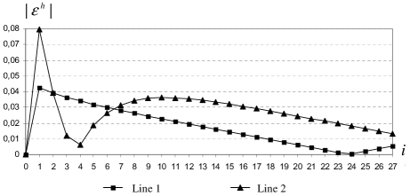
Figure 2: Absolute values of errors in mesh solutions at exactly specified initial data.

Figure 2 was obtained at functions $y_{i}^{h}$ accurately specified in (9), (10). Here, the maximum values of errors made up

$$||\check{\varepsilon}||_{C^{h}}^{N=2}=0.0795,\;||\hat{\varepsilon}||_{C^{h}}^{N=2}=0.0424.$$

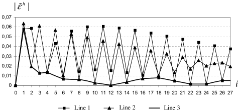
Figure 3: Absolute values of errors in mesh solutions at perturbed initial data.

Figure 3 is obtained at a saw-tooth perturbance of mesh function $y_{i}^{h}$:

$$\tilde{y}(t_{i})=y(t_{i})+(-1)^{i}\,10^{-3},\quad i=\overline{1,27,}\,\,\,\,nh=1.$$

In this case, the maximum values of errors made up

$$||\check{\varepsilon}||_{C^{h}}^{N=2}=0.0638,\;||\hat{\varepsilon}||_{C^{h}}^{N=2}=0.0609,\;||\varepsilon_{\min}||_{C^{h}}^{N=2}=0.0582.$$

Remark. Step $h$ for the fixed level of the initial data perturbances was chosen using the Fibonacci method with ten trials.

The comparison of $\|\check{\varepsilon}^{h}\|_{C_{h}}$ and $\|\hat{\varepsilon}^{h}\|_{C_{h}}$ makes it obvious that the use of the product integration method is more preferable. The computational experiment conducted for the given example at $\alpha=10^{-3}$ shows the convergence for $h<10^{-3}$. In this connection, further studies are supposed to use the numerical methods of higher order, in particular the third- and fourth-order Runge-Kutta methods. Further, it is planned to construct stability regions of the considered algorithms by the analogy with [19].

Conclusion

The paper presents the research into the approximate solution of the Volterra integral equation of the first kind of convolution type, which occurs in the inverse boundary-value heat conduction problem, by the second-order finite difference methods. The calculation results obtained using the system Maple 10 are presented. The computational experiment is conducted in terms of the error occurrence mechanism in computer calculations. Typical cases of systematic error accumulation are demonstrated by the test examples. Software for the calculation of kernels, tracking the valid digits in the significand, is developed in PASCAL.

References

- [1] Brunner H., van der Houwen P.J. The Numerical Solution of Volterra Equations. North-Holland, Amsterdam, 1986.
- [2] Brunner H. Collocation methods for Volterra integtal and related funktional differential equations. N.Y., Cambridge Univ. Press, 2004.
- [3] Verlan’ A.F., Sizikov V.S. Integralnye uravneniya: metody, algoritmy, programmy [Integral equations: methods, algorithms, programs]. Kiev, Nauk. dumka, 1986. (in Russian)
- [4] Apartsyn A.S. Nonclassical linear Volterra equations of the first kind. Boston, VSP Utrecht, 2003.
- [5] Solodusha S.V. [Application of numerical methods for the Volterra equations of the first kind that appear in an inverse boundary-value problem of heat conduction]. Izvestiya IGU. Matematika, 2015, vol. 11, pp. 96–105. (in Russian)
- [6] Solodusha S.V., Yaparova N.M. Numerical solution of the Volterra equations of the first kind that appear in an inverse boundary-value problem of heat conduction. Siberian J. Num. Math, 2015, vol. 18, no. 3, pp. 321–329. DOI: 10.15372/SJNM20150307
- [7] Yaparova N.M. [Numerical simulation for solving an inverse boundary heat conduction problem]. Bulletin of the South Ural University. Mathematical Modelling, Programming and Computer Software, 2013, vol. 6, no. 3, pp. 112–124. (in Russian)
- [8] Jonas P. and Louis A.K. Approximate inverse for a one dimensional inverse heat conduction problem. Inverse Problems, 2000, vol. 16, no. 1, pp. 175–185. DOI: 10.1088/0266-5611/16/1/314
- [9] Prud’homme M. and Hguyen T.H. Fourier analysis of conjugate gradient method applied to inverse heat con-duction problems. International Journal of Heat and Mass Transfer, 1999, vol. 42, pp. 4447–4460. DOI: 10.1016/S0017-9310(99)00112-X
- [10] Kolodziej J. and Mierzwiczak M. and Cialkowski M. Application of the method of fundamental solutions and radial basis functions for inverse heat source problem in case of steady-state. International Communications in Heat and Mass Transfer, vol.37, 2010, no. 2, pp. 21–124. DOI: 10.1016/j.icheatmasstransfer.2009.09.015
- [11] Cialkowski M. and Grysa K. A sequential and global method of solving an inverse problem of heat conduction equation. Jornal of Theoretical and applied Mechanics, 2010, vol. 48, no. 1, pp. 111–134.
- [12] Monde M., Arima H., Liu Wei, Mitutake Yuhichi, Hammad J.A. An analytical solution for two-dimensional inverse heat conduction problems using Laplace transform. International Journal of Heat and Mass Transfer, 2003, vol. 46, pp. 2135–2148. DOI: 10.1016/S0017-9310(02)00510-0.
- [13] Beilina L. and Klibanov M.V. Approximate Global Convergence and Adaptivity for Coefficient Inverse Problems. N.Y., Springer-Verlag, 2012.
- [14] Kabanikhin S.I. Inverse and Ill-Posed Problems. Theory and Applications. Germany, De Gruyter, 2011.
- [15] Kalitkin N.N. Chislennye metody [Numerical methods]. M., Nauka, 1978. (in Russian)
- [16] Mokry I.V., Khamisov O.V., Tsapakh A.S. [The Basic Mechanisms of the Emergence of Computational Errors in Computer Calculations]. Proc. IVth All-Russian Conference «Problems of Optimization and Economic Applications» , Omsk, Nasledie, 2009, pp. 185. (in Russian)
- [17] Linz P. Product integration method for Volterra integral equations of the first kind. BIT, 1971, vol. 11, pp. 413-421.
- [18] Geng F.Z., Cui M.G. Analytical Approximation to Solutions of Singularly Perturbed Boundary Value Problems. Bulletin of the Malaysian Mathematical Sciences Society, 2010, vol. 33, no. 2, pp. 221-232.
- [19] Bulatov M.V., Budnikova O.S. An analysis of multistep methods for solving integral-algebraic equations: construction of stability domains // Computation mathematics and mathematical physics, 2013, vol. 53, no. 9, pp. 1260-1271. DOI: 10.1134/S0965542513070075