Exact formulas for radiative heat transfer between planar bodies under arbitrary
temperature profiles: modified asymptotics and sign-flip transitions

Abstract

We derive exact analytical formulas for the radiative heat transfer between parallel slabs separated by vacuum and subject to arbitrary temperature profiles. We show that, depending on the derivatives of the temperature at points close to the slab–vacuum interfaces, the flux can exhibit one of several different asymptotic low-distance ($d$) behaviors, obeying either $1/d^{2}$, $1/d$, or logarithmic power laws, or approaching a constant. Tailoring the temperature profile within the slabs could enable unprecedented tunability over heat exchange, leading for instance to sign-flip transitions (where the flux reverses sign) at tunable distances. Our results are relevant to the theoretical description of on-going experiments exploring near-field heat transfer at nanometric distances, where the coupling between radiative and conductive heat transfer could be at the origin of temperature gradients.

I Introduction

Two bodies held at different temperatures and separated by vacuum can exchange energy radiatively. At distances $d$ much smaller than the thermal wavelength $\lambda_{T}=\hbar c/k_{B}T$, such radiative heat transfer (RHT) can be orders-of-magnitude larger than the far-field theoretical limits predicted by Planck’s law, a consequence of evanescent tunneling JoulainSurfSciRep05 . This effect is further enhanced in materials supporting polaritonic resonances, leading to a well-known divergence $\sim 1/d^{2}$ of the flux with decreasing vacuum gaps ChapuisPRB08 ; MuletMTE02 . Such a divergence has been confirmed by experiments at sub-micron scales HuApplPhysLett08 ; NarayanaswamyPRB08 ; RousseauNaturePhoton09 ; ShenNanoLetters09 ; KralikRevSciInstrum11 ; OttensPRL11 ; vanZwolPRL12a ; vanZwolPRL12b ; KralikPRL12 ; KimNature15 ; StGelaisNatureNano16 ; SongNatureNano15 , but has been observed and predicted to fail at sub-nanometric distances KittelPRL05 ; KloppstecharXiv . In particular, deviations from the $1/d^{2}$ power law have been predicted to arise in interleaved geometries Rodriguez13 , as well as due to non-local damping HenkelApplPhysB06 ; JoulainJQSRT , acoustic phonon tunneling ChiloyanNatComm15 , and from the interplay of sur- face roughness and curvature Kruger . One unexplored mechanism that could potentially modify RHT are temperature variations: at nanometer gaps (now within experimental reach SongNatureNano15 ; KloppstecharXiv ), the interplay between RHT and conduction can produce temperature gradients within objects MessinaPRB ; JinarXiv , requiring full account of such effects within the quantum-electrodynamics framework FVC ; Eda1 ; Eda2 .

In this work, we derive exact analytical formulas for the RHT between two parallel slabs subject to arbitrary temperature profiles and demonstrate the existence of several asymptotic low-distance $d$ behaviors: depending on the values and derivatives of the temperature profile at points near the slab–vacuum interfaces, the flux can diverge as $1/d^{2}$, $1/d$, or logarithmically, or approach a constant, as $d\to 0$. We show that the temperature profile of the slabs can be tailored so as to modify and even reverse the direction of the flux over tunable distances. As described in MessinaPRB , such temperature gradients can naturally arise due to the interplay of conduction and radiation at nanometric scales, leading to constant (rather than diverging) flux rates as $d\to 0$, even in the absence of phonon or non-local tunneling effects JoulainJQSRT ; ChiloyanNatComm15 . The impact of temperature profile on the properties of RHT remains so far almost unexplored. This tunability could be indeed relevant for the design of thermal devices, such as for example memories devices and thermal rectifiers rect , where the ability to tune the flux dependence on temperature and separation is very important.

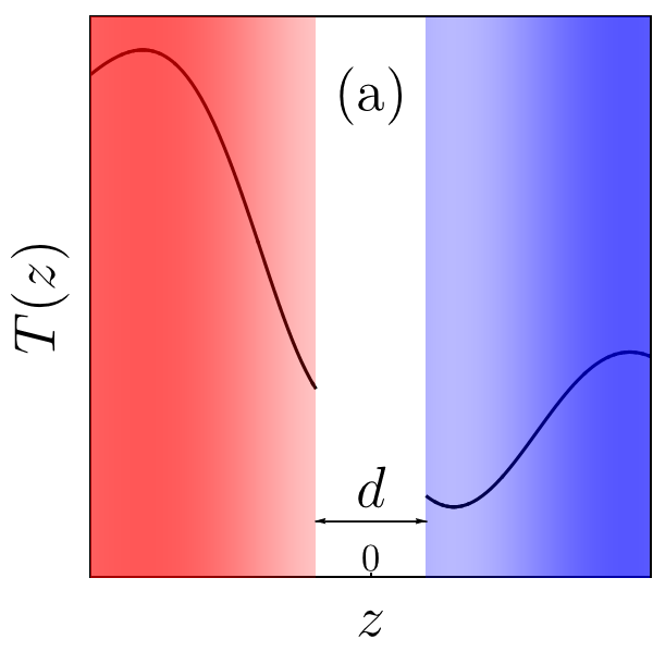
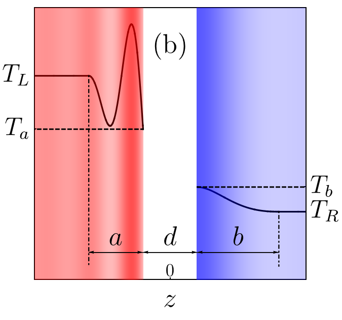
Figure 1: Schematic of two parallel slabs separated by a distance $d$ along the $z$ direction. The two slabs are subject to a temperature profile $T(z)$. Panel (a) depicts the general case of an arbitrary $T(z)$, whereas (b) illustrates a configuration in which the temperatures in the regions $z\leq-d/2-a$ and $z\geq d/2+b$ are held at $T_{L}$ and $T_{R}$, with $T_{a}$ and $T_{b}$ denoting the temperatures at the left and right slab–vacuum interfaces, respectively.

II General formulas

Consider two semi-infinite co-planar slabs a distance $d$ apart and subject to a position-dependent temperature profile $T(z)$, represented in Fig. 1(a). The RHT between the slabs is derived within the framework of the scattering-matrix formalism developed in MessinaPRA11 ; MessinaPRA14 , used previously to describe the Casimir force and RHT in presence of two and three bodies. The first step in our derivation is to express the correlation functions of the electric fields emitted by a single body at temperature $T$ in terms of the reflection and transmission operators of this body. In contrast to MessinaPRA11 , our scenario requires that we apply such a scheme to a film of infinitesimally small thickness $dz$ at a position $z$ of one of the two slabs. The total field emitted by a slab can then be calculated as the sum of these individual fields, including contributions of multiply reflected and transmitted fields from the other portions of the slab, following Refs. MessinaPRA11 ; MessinaPRA14 . Once the field emitted by each slab is statistically characterized, the total field in the vacuum gap can be deduced, allowing us to obtain the Poynting vector or flux per unit area in the gap.

The first step in our derivation is the characterization of the fields emitted by each body, and their correlation functions. Assuming local thermal equilibrium, the statistical properties of the fields radiated by each body depend only on the local temperature within the object. Given a source of thermal fluctuations, the quantity of interest is the symmetrized average $\langle E_{p}^{\phi}(\mathbf{k},\omega)E_{p^{\prime}}^{\phi^{\prime}{\dagger}}(\mathbf{k}^{\prime},\omega^{\prime})\rangle$, where $p$ denotes the polarization, $\phi$ the propagation direction along the $z$ axis, $\mathbf{k}$ the component of the wavevector orthogonal to the $z$ axis, and $\omega$ the frequency, restricted here to positive values.

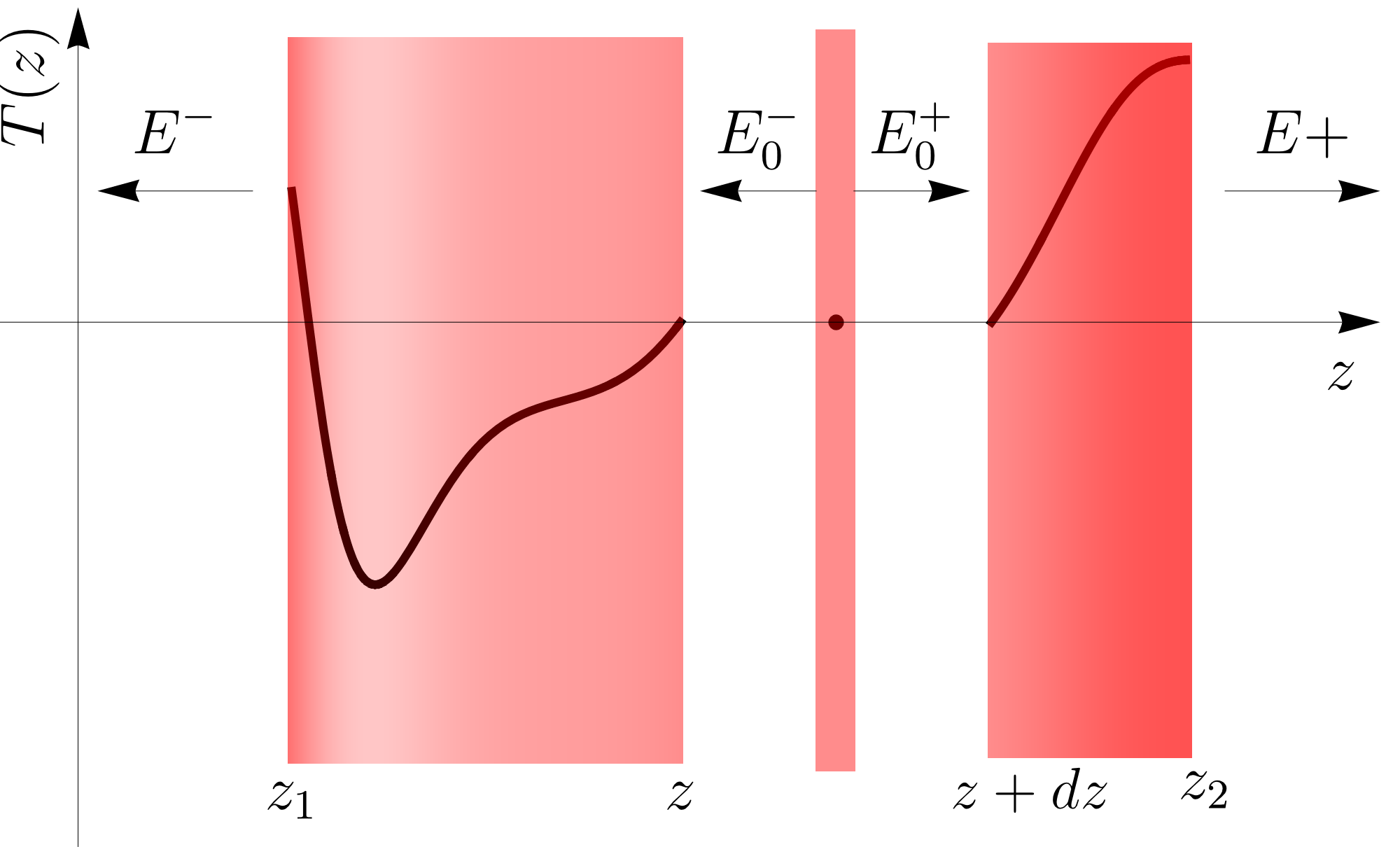
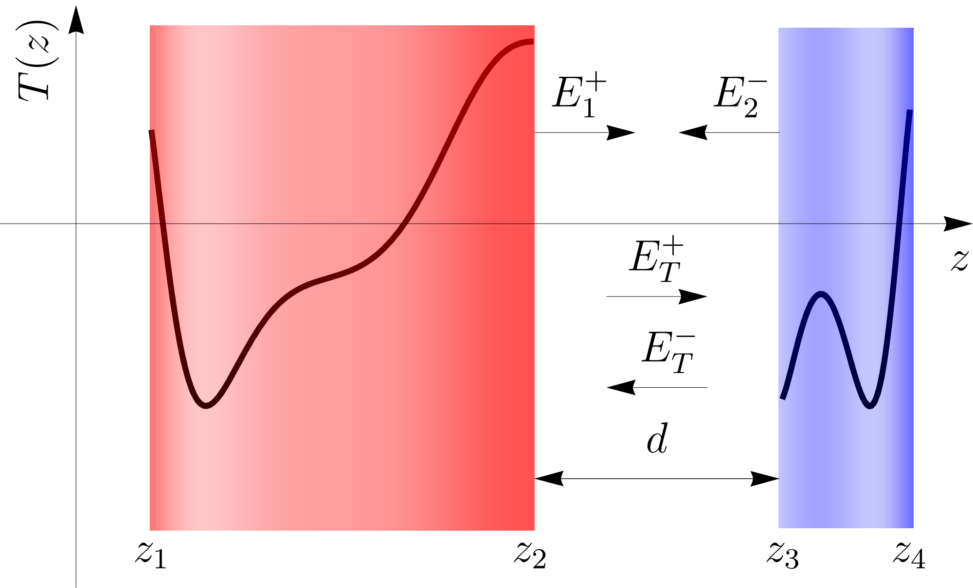
Figure 2: In the upper part, schematic of one slab having a position-dependent temperature $T(z)$. The slab occupies the region $[z_{1},z_{2}]$ and the element from $z$ to $z+dz$ produces the field $E_{0}$. The total field emitted by the slab on the left (right) side is $E^{+}$ ($E^{-}$). In the lower part, two slabs having a temperature profile $T(z)$ and placed at distance $d$. The slab on the left (right) side produces a field $E_{1}$ ($E_{2}$), while the total field inside the cavity has amplitudes $E_{T}^{\pm}$.

Equations (45) and (46) of MessinaPRA11 characterize the correlation function in terms of matrix elements of the reflection and transmission operators at each object interface. In the case of a slab, these matrix elements coincide with the well-known Fresnel coefficients, modified to take into account the possibility of finite slab thickness MessinaPRA14 . In order to incorporate the possibility of varying temperature within a slab, we decompose the slab in terms of infinitesimally thin films (see Fig. 2) and apply these correlation formulas to an arbitrary film located at $z$ and having thickness $dz$. Specifically, given some arbitrary position $z$, we replace the modified Fresnel coefficients with their first-order series expansion in terms of the thickness $dz$ of the corresponding film, given by:

$$\begin{split}\rho&\simeq-i\frac{2k_{zm}r}{1-r^{2}}dz,\\ \tau&\simeq 1-i\Bigl{(}k_{z}-k_{zm}\frac{1+r^{2}}{1-r^{2}}\Bigr{)}dz,\end{split}$$ (1)

where $k_{z}$ ($k_{zm}$) is the $z$ component of the wavevector in vacuum (or the medium), and $r$ is the ordinary Fresnel coefficient. It follows that the correlation function of the field $E_{0}$ emitted by the film is given by:

$$\begin{split}\langle E_{0,p}^{\phi}(\mathbf{k},\omega)E_{0,p^{\prime}}^{\phi^{\prime}{\dagger}}(\mathbf{k}^{\prime},\omega^{\prime})&=\frac{\omega\,dz}{2\varepsilon_{0}c^{2}}N[\omega,T(z)](2\pi)^{3}\delta(\omega-\omega^{\prime})\\ &\,\times\delta(\mathbf{k}-\mathbf{k}^{\prime})\delta_{pp^{\prime}}\mathcal{F}_{0,p}^{\phi\phi^{\prime}}(\mathbf{k},\omega).\end{split}$$ (2)

More precisely, the field correlations involving waves traveling in the same ($\phi^{\prime}-=\phi$) or opposite ($\phi^{\prime}=-\phi$) directions are given by:

$$\begin{split}\mathcal{F}_{0,p}^{\phi\phi}(\mathbf{k},\omega)&=\Theta(\omega-ck)\frac{2}{k_{z}}\operatorname{Im}\Bigl{(}k_{zm}\frac{1+r^{2}}{1-r^{2}}\Bigr{)}\\ &\,-\Theta(ck-\omega)\frac{4}{\operatorname{Im}(k_{z})}\operatorname{Re}\Bigl{(}\frac{k_{zm}r}{1-r^{2}}\Bigr{)}e^{2\phi\operatorname{Im}(k_{z})z},\\ \mathcal{F}_{0,p}^{\phi,-\phi}(\mathbf{k},\omega)&=-\Theta(\omega-ck)\frac{4}{k_{z}}\operatorname{Im}\Bigl{(}\frac{k_{zm}r}{1-r^{2}}\Bigr{)}e^{-2i\phi k_{z}z}\\ &\,+\Theta(ck-\omega)\frac{2}{\operatorname{Im}(k_{z})}\operatorname{Re}\Bigl{(}k_{zm}\frac{1+r^{2}}{1-r^{2}}\Bigr{)},\end{split}$$ (3)

which are both diagonal with respect to $\omega$, $\mathbf{k}$, and $p$ due to the time- and translation-invariance characterizing the slab. Furthermore, it is proportional to $dz$, and thus goes to zero in absence of the film.

Equations (2) and (3) fully characterize the field $E_{0}$ emitted by the film. The counterpropagating components $E^{\pm}$ of the total field can be expressed as the sum of the individual contributions of each film, each of which experiences multiple reflections and transmissions at slab interfaces. The contribution of a given film of thickness $dz$ reads,

$$\begin{cases}E^{+}=u(z_{1},z_{2})\tau(z_{2}-z)\Bigl{(}E_{0}^{+}+\rho(z-z_{1})e^{-2ik_{z}z}E_{0}^{-}\Bigr{)},\\ E^{-}=u(z_{1},z_{2})\tau(z-z_{1})\Bigl{(}\rho(z_{2}-z)e^{2ik_{z}z}E_{0}^{+}+E_{0}^{-}\Bigr{)},\end{cases}$$ (4)

where $\rho(\delta)$ and $\tau(\delta)$ are the reflection and transmission coefficients of a slab of thickness $\delta$ (defined as in MessinaPRA14 ), and $u(z_{1},z_{2})=[1-\rho(z-z_{1})\rho(z_{2}-z)]^{-1}$. In order to deduce the RHT between the two slabs, we require the correlation functions for co-propagating components $\langle E_{1}^{+}E_{1}^{+{\dagger}}\rangle$ and $\langle E_{2}^{-}E_{2}^{-{\dagger}}\rangle$ emitted by the two slabs (see Fig. 2). These can be easily obtained from Eqs. (2), (3), and (4). Defining $\mathcal{F}_{i,p}^{\phi\phi^{\prime}}(\mathbf{k},\omega)$ for fields $E_{i}$ produced by each slab ($i=1,2$) as

$$\begin{split}\langle E_{i,p}^{\phi}(\mathbf{k},\omega)E_{i,p^{\prime}}^{\phi^{\prime}{\dagger}}(\mathbf{k}^{\prime},\omega^{\prime})&=\frac{\omega}{2\varepsilon_{0}c^{2}}(2\pi)^{3}\delta(\omega-\omega^{\prime})\\ &\,\times\delta(\mathbf{k}-\mathbf{k}^{\prime})\delta_{pp^{\prime}}\mathcal{F}_{i,p}^{\phi\phi^{\prime}}(\mathbf{k},\omega),\end{split}$$ (5)

we obtain:

$$\begin{split}\mathcal{F}_{1}^{++}&=\int_{z_{1}}^{z_{2}}\!\!dz\,N[\omega,T(z)]|\tau(z_{2}-z)u(z_{1},z_{2})|^{2}\Bigl{[}\mathcal{F}_{0}^{++}+\rho^{*}(z-z_{1})e^{2ik^{*}_{z}z}\mathcal{F}_{0}^{+-}\\ &\hskip 170.71652pt+\rho(z-z_{1})e^{-2ik_{z}z}\mathcal{F}_{0}^{-+}+|\rho(z-z_{1})e^{-2ik_{z}z}|^{2}\mathcal{F}_{0}^{--}\Bigr{]},\\ \mathcal{F}_{2}^{--}&=\int_{z_{3}}^{z_{4}}\!\!dz\,N[\omega,T(z)]|\tau(z-z_{3})u(z_{3},z_{4})|^{2}\Bigl{[}|\rho(z_{4}-z)e^{2ik_{z}z}|^{2}\mathcal{F}_{0}^{++}+\rho(z_{4}-z)e^{2ik_{z}z}\mathcal{F}_{0}^{+-}\\ &\hskip 170.71652pt+\rho^{*}(z_{4}-z)e^{-2ik^{*}_{z}z}\mathcal{F}_{0}^{-+}+\mathcal{F}_{0}^{--}\Bigr{]},\\ \end{split}$$ (6)

where for simplicity we have assumed that the two slabs are made of the same material.

Following Ref. MessinaPRA11 , the flux through a unit area of the $zz$ component of the Poynting vector in the vacuum region between the two slabs can be expressed in terms of correlation functions of the total field $E_{T}$ between the two slabs as:

$$\begin{split}\varphi=\frac{1}{(2\pi)^{2}}\sum_{p}\int_{0}^{+\infty}\!\!&d\omega\Biggl{[}\int_{0}^{\frac{\omega}{c}}\!\!dk\,k\,k_{z}\bigl{(}\mathcal{F}_{T}^{++}-\mathcal{F}_{T}^{--}\bigr{)}+\int_{\frac{\omega}{c}}^{+\infty}\!\!dk\,k\,i\,\mathrm{Im}(k_{z})\bigl{(}\mathcal{F}_{T}^{+-}-\mathcal{F}_{T}^{-+}\bigr{)}\Biggr{]}.\end{split}$$ (7)

with the total field $E_{T}$ itself written as the result of multiple reflections of $E_{1}^{+}$ and $E_{2}^{-}$ as:

$$\begin{cases}E_{T}^{+}=u_{23}\Bigl{(}E_{1}^{+}+\rho(z_{2}-z_{1})e^{-2ik_{z}z_{2}}E_{2}^{-}\Bigr{)},\\ E_{T}^{-}=u_{23}\Bigl{(}\rho(z_{4}-z_{3})e^{2ik_{z}z_{3}}E_{1}^{+}+E_{2}^{-}\Bigr{)},\end{cases}$$ (8)

being $u_{23}=[1-\rho(z_{2}-z_{1})\rho(z_{4}-z_{3})e^{2ik_{z}d}]^{-1}$. The total correlation functions are therefore given by:

$$\begin{split}\mathcal{F}_{T}^{++}&=|u_{23}|^{2}\Bigl{(}\mathcal{F}_{1}^{++}+|\rho(z_{2}-z_{1})e^{-2ik_{z}z_{2}}|^{2}\mathcal{F}_{2}^{--}\Bigr{)},\\ \mathcal{F}_{T}^{+-}&=|u_{23}|^{2}\Bigl{(}\rho^{*}(z_{4}-z_{3})e^{-2ik^{*}_{z}z_{3}}\mathcal{F}_{1}^{++}+\rho(z_{2}-z_{1})e^{-2ik_{z}z_{2}}\mathcal{F}_{2}^{--}\Bigr{)},\\ \mathcal{F}_{T}^{-+}&=|u_{23}|^{2}\Bigl{(}\rho(z_{4}-z_{3})e^{2ik_{z}z_{3}}\mathcal{F}_{1}^{++}+\rho^{*}(z_{2}-z_{1})e^{2ik_{z}^{*}z_{2}}\mathcal{F}_{2}^{--}\Bigr{)},\\ \mathcal{F}_{T}^{--}&=|u_{23}|^{2}\Bigl{(}|\rho(z_{4}-z_{3})e^{2ik_{z}z_{3}}|^{2}\mathcal{F}_{1}^{++}+\mathcal{F}_{2}^{--}\Bigr{)},\end{split}$$ (9)

The above expressions can be simplified in the case of two slabs of infinite thickness ($z_{1}\to-\infty$ and $z_{4}\to+\infty$), in which case $\rho(\delta)$ becomes the ordinary Fresnel coefficient $r$. In Eq. (7) the flux is written as an integral $\varphi=\int_{0}^{+\infty}d\omega\,\varphi(\omega)$, with the spectral components at frequency $\omega=ck_{0}$ broken down into contributions from propagative waves $(\omega>ck)$ and evanescent $(\omega<ck)$ waves. Using Eq. (9) and after algebraic manipulations we get the following results for propagative waves

$$\varphi_{\text{pw}}(\omega)=\frac{1}{2\pi^{2}}\int_{0}^{k_{0}}\!\!dk\,k\frac{(1-|r|^{2})^{2}k^{\prime\prime}_{zm}}{|1-r^{2}e^{2ik_{z}d}|^{2}}\int_{0}^{+\infty}\!\!\!\!\!dz\,e^{-2k^{\prime\prime}_{zm}z}\Bigl{\{}N\Bigl{[}\omega,T\bigl{(}-\frac{d}{2}-z\bigr{)}\Bigr{]}-N\Bigl{[}\omega,T\bigl{(}\frac{d}{2}+z\bigr{)}\Bigr{]}\Bigr{\}},$$ (10)

and for evanescent waves

$$\varphi_{\text{ew}}(\omega)=\frac{2}{\pi^{2}}\int_{k_{0}}^{+\infty}\!\!\!\!dk\,k\frac{(r^{\prime\prime})^{2}e^{-2k_{z}^{\prime\prime}d}k^{\prime\prime}_{zm}}{|1-r^{2}e^{-2k_{z}^{\prime\prime}d}|^{2}}\int_{0}^{+\infty}\!\!\!\!\!dz\,e^{-2k^{\prime\prime}_{zm}z}\Bigl{\{}N\Bigl{[}\omega,T\bigl{(}-\frac{d}{2}-z\bigr{)}\Bigr{]}-N\Bigl{[}\omega,T\bigl{(}\frac{d}{2}+z\bigr{)}\Bigr{]}\Bigr{\}},$$ (11)

where $N(\omega,T)=\hbar\omega/[\exp(\hbar\omega/k_{B}T)-1]$ denotes the Planck energy of a thermal oscillator, and $c^{\prime},c^{\prime\prime}$ denote the real and imaginary parts of the complex number $c$. As expected, our expressions simplify in the limit of uniform temperature, reproducing the typically derived formulas for RHT JoulainSurfSciRep05 (note that in addition to the spatial integral over the temperature profiles, our result differs from the typical RHT formula by the extra factor $k^{\prime\prime}_{zm}$ in the numerator).

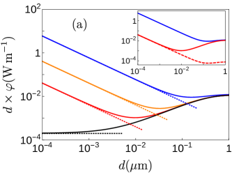
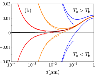
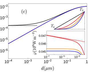
Figure 3: (a) Heat flux (multiplied by $d$) between two SiC slabs, shown schematically in Fig. 1(b), separated by a distance $d$ and subject to several temperature configurations. In all cases, $a=b=1\,\mu$m and $(T_{L},T_{R})=(600,300)\,$K. Top to bottom plots correspond to $(T_{a},T_{b})=(600,300)\,$K (blue), $(460,440)\,$K (orange), $(451,449)\,$K (red) and $(450,450)\,$K (black). Also shown are the predictions (dot-dashed lines) of the asymptotic formulas given in (14) and (15). The inset compares the flux corresponding to the case $(T_{L},T_{a},T_{b},T_{R})=(600,451,449,300)\,$K against two uniform-temperature configurations $(600,600,300,300)\,$K (solid blue line) and $(451,451,449,449)\,$K (dashed red line). (b) Same curves in (a) but plotted in a linear scale, with the addition of three configurations (dashed lines): $(T_{a},T_{b})=(449,451)\,$K (red), $(440,460)\,$K (orange) and $(300,600)\,$K (blue). (c) Heat flux associated with the temperature configuration $(T_{L},T_{a},T_{b},T_{R})=(600,450,450,300)\,$K but under different temperature variations (top inset), described as polynomials of orders $n$, corresponding to linear ($n=1$, black), quadratic ($n=2$, red), cubic ($n=3$, orange), or quartic ($n=4$, blue) polynomials. The black dot-dashed line shows the asymptotic behavior predicted by (15). The bottom inset illustrates the asymptotic behavior of the $n>1$ profiles, with the red dot-dashed line corresponding to the prediction of (17).

III Asymptotic behavior

We are interested in studying the impact of temperature gradients in the asymptotic limit $d\to 0$, in which case RHT is dominated by evanescent contributions from the transverse-magnetic polarization. Taylor expanding the population functions around the slab–vacuum interfaces,

$$N\Bigl{[}\omega,T\bigl{(}\pm\frac{d}{2}\pm z\bigr{)}\Bigr{]}=\sum_{n=0}^{+\infty}\frac{\alpha^{\pm}_{n}(\omega)}{n!}z^{n},$$ (12)

we obtain the RHT $\varphi(\omega)=\sum_{n}\varphi_{n}(\omega)$ in increasing orders of the temperature away from the interface, with

$$\begin{split}&\varphi_{n}(\omega)=\frac{\alpha^{-}_{n}(\omega)-\alpha^{+}_{n}(\omega)}{2^{n}\pi^{2}}\int_{k_{0}}^{+\infty}\!\!\!\!\frac{k\,dk}{(k^{\prime\prime}_{zm})^{n}}\frac{(r^{\prime\prime})^{2}e^{-2k^{\prime\prime}_{z}d}}{|1-r^{2}e^{-2k^{\prime\prime}_{z}d}|^{2}}.\end{split}$$ (13)

Since the integrand behaves as $k^{1-n}$, it follows that terms of order $n\geq 3$ contribute finite RHT whereas those of order ${n=0,1,2}$ diverge in the limit $d\to 0$. Such a divergence is associated with the increasing contribution of large-$k$ states, allowing us to approximate the integral. In this limit, $k^{\prime\prime}_{zm}\simeq k$, $r$ approaches the $k$-independent quantity $(\varepsilon(\omega)-1)/(\varepsilon(\omega)+1)$, and it is possible to take the limit $k_{0}\to 0$, allowing us to perform the various $k$ integrals explicitly. Specifically, performing the change of variable $x=e^{-2kd}$, we obtain:

$$\varphi_{0}(\omega)\simeq\frac{1}{8\pi^{2}d^{2}}\frac{r^{\prime\prime}}{r^{\prime}}\operatorname{Im}[\text{Li}_{2}(r^{2})][\alpha^{-}_{0}(\omega)-\alpha^{+}_{0}(\omega)],$$ (14)

where $\alpha^{-}_{0}(\omega)-\alpha^{+}_{0}(\omega)=N(\omega,T_{a})-N(\omega,T_{b})$ and $\text{Li}_{n}(z)=\sum_{k=1}^{+\infty}z^{k}/k^{n}$ is the polylogarithmic function. Hence, one finds that to zeroth order in the gradient expansion at the interface, the RHT $\sim 1/d^{2}$ as $d\to 0$ whenever $T_{a}\neq T_{b}$. In contrast, if the temperatures at the interfaces coincide, this divergence is regularized and the leading contribution instead comes from the $n=1$ term, given by:

$$\varphi_{1}(\omega)\simeq-\frac{1}{8\pi^{2}d}\frac{r^{\prime\prime}}{r^{\prime}}\operatorname{Im}[\log(1-r^{2})][\alpha^{-}_{1}(\omega)-\alpha^{+}_{1}(\omega)].$$ (15)

where, assuming $T_{a}=T_{b}$, one finds that $\alpha^{-}_{1}(\omega)-\alpha^{+}_{1}(\omega)=-[\partial_{z}T(-d/2)+\partial_{z}T(d/2)]\partial_{T}N(\omega,T_{a})$ depends on the derivatives of the temperature profile at $z=\pm d/2$. It follows that if $\partial_{z}T(-d/2)\neq-\partial_{z}T(d/2)$ and $T_{a}=T_{b}$, the asymptotic behavior of the RHT $\sim 1/d$. If the former is violated, e.g. when the profile has zero derivative at the interfaces, then the $n=1$ term is exactly zero, and the asymptotic behavior is instead determined by the $n=2$ term, which requires a more delicate treatment. In particular, replacing the integrand by its high-$k$ behavior and performing a different change of variables $x=\log(ck/\omega)/\log(\omega d/c)$, one finds:

$$\varphi_{2}(\omega)\simeq-\frac{[\operatorname{Im}(r)]^{2}}{4\pi^{2}}\log\Bigl{(}\frac{\omega d}{c}\Bigr{)}[\alpha^{-}_{2}(\omega)-\alpha^{+}_{2}(\omega)]\\ \times\int_{-\infty}^{0}dx\,\frac{e^{-2k(x)d}}{|1-r^{2}e^{-2k(x)d}|^{2}},$$ (16)

with $k(x)\equiv k_{0}\exp[\log(\omega d/c)x]$. We now observe that as $d\to 0$, the function $\exp[-2k(x)d]$ tends to 1 for any ${-1<x<0}$ and to 0 for any $x<-1$. Thus, if $T_{a}=T_{b}$ and $\partial_{z}T(-d/2)=-\partial_{z}T(d/2)$, it follows that

$$\varphi_{2}(\omega)\simeq-\frac{1}{4\pi^{2}}\log\Bigl{(}\frac{\omega d}{c}\Bigr{)}\frac{(r^{\prime\prime})^{2}}{|1-r^{2}|^{2}}[\alpha^{-}_{2}(\omega)-\alpha^{+}_{2}(\omega)].$$ (17)

where $\alpha^{-}_{2}(\omega)-\alpha^{+}_{2}(\omega)=[\partial^{2}_{z}T(-d/2)-\partial^{2}_{z}T(d/2)]\partial_{T}N(\omega,T_{a})$ involves only second derivatives of $T(z)$ at $z=\pm d/2$. Such a logarithmic divergence is further regularized if $\partial^{2}_{z}T(-d/2)=\partial^{2}_{z}T(d/2)$, in which case the RHT tends to a constant value in the limit $d\to 0$. A trivial situation under which all three conditions lead to constant flux as $d\to 0$ is an even temperature profile, i.e. $T(-z)=T(z)$, in which case the flux vanishes at every $d$.

IV Numerical predictions

In order to discuss the rich scenarios associated with the presence of temperature gradients, we consider numerical evaluation of the above formulas for the case of two infinitely thick parallel silicon carbide (SiC) slabs separated by vacuum. We consider the specific configuration depicted in Fig. 1(b), in which the temperature of the slab on the left (right) is constant and equal to $T_{L}$ ($T_{R}$) everywhere except for a region of thickness $a$ ($b$), with $T_{a}$ ($T_{b}$) denoting the slab–vacuum interface temperatures of the left (right) slab. Such a scenario would arise, for instance, if both slabs were to be connected to thermal reservoirs held at $T_{L}$ and $T_{R}$. The dielectric properties of SiC are described by means of a Drude-Lorenz model Palik98 , highlighting the existence of a surface phonon-polariton resonance in the infrared region of the spectrum, particularly relevant for near-field RHT JoulainSurfSciRep05 . We fix $a=b=1\,\mu$m, focusing first on the case $(T_{L},T_{R})=(600,300)\,$K and assuming a linear temperature gradient in the regions of varying temperature, determined by our choice of $T_{a}$ and $T_{b}$.

Figure 3(a) shows the RHT (multiplied by $d$) over a wide range of $d\in[10^{-4},1]\,\mu$m. Note that we include extremely low values of separations (below a nanometer) in order to better illustrate the asymptotic regimes discussed above. We consider three configurations in which $T_{a}$ differs from $T_{b}$, illustrating the expected $1/d^{2}$ scaling described by (14), plotted as dotted lines, the appearance of which depends on the precise values of $T_{a}$ and $T_{b}$, with the transition occuring anywhere between a few to hundreds of nm. Also shown is the RHT in the special case ${T_{a}=T_{b}=450\,}$K, illustrating the $1/d$ behavior predicted by (15) (dotted line), the onset of which occurs below the nm scale. Noticeably, while all four curves approach one another at the micron scale, the different values of interface temperatures produce both quantitatively and qualitatively different behaviors in the experimentally accessible range ${d\in[1,100]\,}$nm. It is instructive to compare one of the above configurations, $(T_{L},T_{a},T_{b},T_{R})=(600,451,449,300)\,$K, to the more standard scenario of uniform-temperature slabs: $(600,600,300,300)\,$K and $(451,451,449,449)\,$K. The results, shown in the inset of Fig. 3(a), demonstrate that at small distances, RHT becomes a surface effect, in which case only the interface temperatures are relevant; in contrast, at large $d$ RHT is dominated (and well described) by the bulk temperatures $T_{L}$ and $T_{R}$ of the infinite regions.

Figure 3(b) shows the four curves of Fig. 3(a) in a linear scale and introduces three additional configurations, corresponding to situations in which $T_{a}\leftrightarrow T_{b}$ are exchanged (dashed lines). Such a flip leads to a situation in which the bulk ($T_{L}>T_{R}$) and surface ($T_{a}<T_{b}$) temperatures compete, contributing RHT in opposite directions. As before, the behavior at asymptotically small $d$ is determined by (14) and (15) (dotted lines), except that in the case of flipped $T_{a}<T_{b}$ (dashed lines), the RHT goes from positive to negative (reversing sign) as $d$ decreases, with the transition distance occuring anywhere from a few to hundreds of nm, depending on $T_{a},T_{b}$. Such a surface-temperature inversion could potentially be engineered (and tuned) via the introduction of an external pump or thermostat.

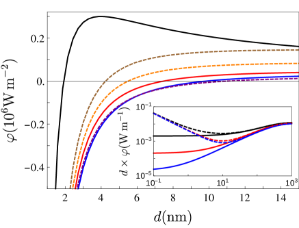
Figure 4: Heat flux as a function of distance for $(T_{a},T_{b},T_{L})=(451,449,300)\,$K. The solid lines correspond to $T_{L}=600\,$K and have $a=b=100\,$nm (black), $1\,\mu$m (red) and $10\,\mu$m (blue). The dashed lines correspond to $a=b=1\,\mu$m and have $T_{L}=800\,$K (brown), $700\,$K (orange) and $500\,$K (purple).

The results presented thus far highlight the existence of both $1/d^{2}$ and $1/d$ asymptotic power-laws. Figure 3(c) on the other hand also illustrates the appearance of logarithmic behavior by considering a situation consisting of fixed $(T_{L},T_{a},T_{b},T_{R})=(600,450,450,300)\,$K but where the intervening temperature profile is chosen to have different polynomial dependencies (shown on the top inset), including linear ($n=1$, black), quadratic ($n=2$, red), cubic ($n=3$, orange), and quartic ($n=4$, blue) power laws. While the sub-$1/d$ behavior associated with the $n>1$ profiles is apparent from the main plot, the three curves are better distinguished in the inset of the figure, which shows the slow, logarithmic scaling associated with the $n=2$ profile, plotted in conjunction with the predictions of (17) (dotted line), along with the fact that RHT approaches a constant for $n>2$.

Figure 4 focuses on the role of the thicknesses ${a=b}$ and external temperature $T_{L}$ on the sign-flip effect explored in Fig. 3(b), considering the reference scenario $(T_{L},T_{a},T_{b},T_{R})=(600,451,449,300)\,$K. We first fix ${T_{L}=600\,}$K and vary the thickness, from $a=100$ nm to $a=10\,\mu$m (black, red, and blue lines), demonstrating a decreasing zero-flux distance, from 10nm to 2nm, with decreasing thickness. Fixing $a=1\,\mu$m and modifying instead the external temperature, from $T_{L}=500\,$K to ${T_{L}=800\,}$K, produces similar variations on the zero-flux distance, from 4nm to 10nm. The inset of Fig. 4 yields even more insights on ways of manipulating the asymptotic behavior, showing the RHT (multiplied by $d$) for the same three values of ${a=100\,\text{nm},1\,\mu\text{m},10\,\mu\text{m}}$ explored in the main figures, but under different surface temperatures (or gradients). The dashed lines correspond to the case $(T_{a},T_{b})=(451,449)\,$K, illustrating the expected $1/d^{2}$ scaling behavior. It follows from (14) that in this case the asymptotic RHT depends only on the two temperatures $T_{a}$ and $T_{b}$ and not on their derivatives, which explains why the three dashed lines approach one another as $d\to 0$. The solid lines correspond to the case $T_{a}=T_{b}=450\,$K and illustrate the expected $1/d$ behavior, revealing an asymptotic prefactor that decreases with decreasing temperature gradients, as predicted by (15).

V Conclusions

The approach we presented, valid for arbitrary materials and distances and based on a scattering-matrix formalism, leads to analytical expressions of the short-distance behavior of the flux. We have shown that the latter is entirely determined by the gradient expansion of the temperature profile near the slab–vacuum interfaces. In particular, we find that apart from the well-known $1/d^{2}$ power-law scaling, under certain conditions, the flux can diverge asymptotically either as $1/d$ or logarithmically, or it can also saturate to a constant value. We have shown that the introduction of a temperature profile can result in significant flux tunability, leading for instance to changes in the sign of the flux with respect to slab separations. The temperature profile within a given body can be for example experimentally engineered by means of the introduction of several thermostats put in contact at different points of the body. Moreover, a temperature gradient can naturally appear as the result of the coupling between radiative exchange and conduction within each body, as studied in detail in Refs. MessinaPRB ; JinarXiv , in both planar and structured geometries. It has been shown that, depending on the chosen material, an observable temperature profile can indeed appear for distances as high as tens or hundreds of nanometers. Our approach would be needed to accurately describe radiative heat transfer under these conditions. In fact, recent experiments are beginning to explore such short distance regime (down to sub-nanometer separations KittelPRL05 ; KloppstecharXiv ; ShenNanoLetters09 ; KimNature15 ), some of which have already observed a saturating flux that has yet to be properly explained. Moreover, the possibility of tuning the temperature profile of a system and thereby the behavior, e.g. sign, of the heat transfer with respect to external thermal sources is yet unexplored and could be important for thermal devices devices . Finally, it must be stressed that at distances as low as a few nanometers or in the sub-nanometer range theoretical descriptions based on macroscopic fluctuational electrodynamics are no longer valid: in this regime, atomic-scale and other non-local screening effects as well as the tunneling of phonons can play significant role.

References

- (1) K. Joulain et al., Surf. Sci. Rep. 57, 59 (2005).
- (2) P.-O. Chapuis et al., Phys. Rev. B 77, 035431 (2008).
- (3) J.-P. Mulet, K. Joulain, R. Carminati, and J.-J.Greffet, Microscale Thermophysical Engineering 6, 209 (2002).
- (4) A. Narayanaswamy, S. Shen, and G. Chen, Phys. Rev. B 78, 115303 (2008).
- (5) L. Hu, A. Narayanaswamy, X. Chen, and G. Chen, Appl. Phys. Lett. 92, 133106 (2008).
- (6) S. Shen, A. Narayanaswamy, and G. Chen, Nano Letters 9, 2909 (2009).
- (7) E. Rousseau, A. Siria, G. Joudran, S. Volz, F. Comin, J. Chevrier, and J.-J. Greffet, Nature Photon. 3, 514 (2009).
- (8) R. S. Ottens, V. Quetschke, S. Wise, A. A. Alemi, R. Lundock, G. Mueller, D. H. Reitze, D. B. Tanner, and B. F. Whiting, Phys. Rev. Lett. 107, 014301 (2011).
- (9) T. Kralik, P. Hanzelka, V. Musilova, A. Srnka, and M. Zobac, Rev. Sci. Instrum. 82, 055106 (2011).
- (10) T. Kralik, P. Hanzelka, M. Zobac, V. Musilova, T. Fort, and M. Horak, Phys. Rev. Lett. 109, 224302 (2012).
- (11) P. J. van Zwol, L. Ranno, and J. Chevrier, Phys. Rev. Lett. 108, 234301 (2012).
- (12) P. J. van Zwol, S. Thiele, C. Berger, W. A. de Heer, and J. Chevrier, Phys. Rev. Lett. 109, 264301 (2012).
- (13) B. Song et al., Nature Nanotechnology 10, 253 (2015).
- (14) K. Kim et al., Nature 528, 387 (2015).
- (15) R. St-Gelais, L. Zhu, S. Fan, and M. Lipson, Nature Nanotechnology 11, 515 (2016).
- (16) A. Kittel, W. Müller-Hirsch, J. Parisi, S.-A. Biehs, D. Reddig, and M. Holthaus, Phys. Rev. Lett. 95, 224301 (2005).
- (17) K. Kloppstech et al., preprint arXiv:1510.06311 (2015).
- (18) A. W. Rodriguez, M. T. H. Reid, J. Varela, J. D. Joannopoulos, F. Capasso, and S. G. Johnson, Phys. Rev. Lett. 110, 014301 (2015).
- (19) C. Henkel and K. Joulain, Appl. Phys. B 84, 61 (2006).
- (20) K. Joulain, J. Quant. Spectrosc. Radiat. Transfer 109, 294 (2008).
- (21) V. Chiloyan, J. Garg, K. Esfarjani, and G. Chen, Nature Comm. 6, 6755 (2015).
- (22) M. Krüger, V. A. Golyk, G. Bimonte, and M. Kardar, Europhys. Lett. 104, 41001 (2013).
- (23) R. Messina, W. Jin, and A. W. Rodriguez, Phys. Rev. B 94, 121410(R) (2016).
- (24) W. Jin, R. Messina, and A. W. Rodriguez, preprint arXiv:1605.05708 (2016).
- (25) A. G. Polimeridis, M. T. H. Reid, W. Jin, S. G. Johnson, J. K. White, and A. W. Rodriguez, Phys. Rev. B 92,134202 (2015).
- (26) S. Edalatapour and M. Francoeur, J. Quant. Spectrosc. Radiat. Transfer 133, 364 (2014).
- (27) S. Edalatapour and M. Francoeur, Phys. Rev. B 94, 045406 (2016).
- (28) P. Ben-Abdallah and S.-A. Biehs, AIP Advances 5, 053502, (2015).
- (29) L. Zhu, C. R. Otey, and S. Fan, Appl. Phys. Lett. 100, 044104 (2012).
- (30) R. Messina and M. Antezza, Phys. Rev. A 84, 042102 (2011).
- (31) R. Messina and M. Antezza, Phys. Rev. A 89, 052104 (2014).
- (32) Handbook of Optical Constants of Solids, edited by E. Palik (Academic Press, New York, 1998).