Linear and anomalous front propagation in system with non Gaussian diffusion: the importance of tails

Abstract

We investigate front propagation in systems with diffusive and sub-diffusive behavior. The scaling behavior of moments of the diffusive problem, both in the standard and in the anomalous cases, is not enough to determine the features of the reactive front. In fact, the shape of the bulk of the probability distribution of the transport process, which determines the diffusive properties, is important just for pre-asymptotic behavior of front propagation, while the precise shape of the tails of the probability distribution determines asymptotic behavior of front propagation.

I Introduction

Reaction-diffusion processes appear in a large class of phenomena from combustion to ecology neufeld2010 . In presence of non trivial geometry (e.g. graphs) burioni2005 or anomalous diffusion processes Barkai2014 ; Klafter2015 the reaction dynamics is an intriguing and difficult issue mancinelli2002 ; mancinelli2003 ; burioni2012 .

In particular, the case of reaction in subdiffusive systems Sokolov2006 ; Mendez2009 ; Fedotov2010 ; Volpert2013 is rather interesting for its role in living systems, since anomalous subdiffusion has been reported for different biological transport problems such as two-dimensional diffusion in the plasma membrane and three-dimensional diffusion in the nucleus and cytoplasm (see Saxton2007 and reference therein).

The aim of the present work is to show that the behavior of tails of the probability distribution of the pure transport problem has the most important role for the front propagation properties, which can be anomalous even in case of standard diffusion. On the other hand one can have the standard linear front propagation also in presence of subdiffusion. It is important to stress that, as already noted in Sokolov2006 ; Mendez2009 and clearly stated in Nepomnyashchy2016 , the details of the reaction-diffusion rules can be very important for the front propagation features.

The paper is organized as follows: in Sect. II we briefly summarize some results about non standard diffusive systems and front propagation in presence of reaction. Sect. III is devoted to an analysis of front propagation in a simplified model with sub-diffusion. In Sect. IV we show that, even in a more realistic model, the basic ingredient for the asymptotic behavior of front propagation is given by the shape of the tail of the probability distribution, $P(x,t)$, of the pure transport problem. We point out that the shape of the bulk of $P(x,t)$, which determines the diffusive properties, could be important just for the pre-asymptotic behavior of the front propagation. Sect. V is dedicated to the conclusions.

II A survey of known results

Let us indicate with $P(x,t)$ the probability distribution (or the probability density) that a walker is in $x$ at time $t$. Under rather general hypothesis, $P(x,t)$ satisfies the equation

$$P(x,t+\Delta t)=\int_{-\infty}^{+\infty}P(x-u,t)\rho_{\Delta t}(u,x,t)du,$$ (1)

where $\rho_{\Delta t}(u,x,t)$ is the probability density to be in $x$ at time $t+\Delta t$ under the condition to be in $x-u$ at time $t$. Even if $\rho_{\Delta t}(u,x,t)$ has an explicit dependence on $x$ and $t$ the process is Markovian. When $\rho_{\Delta t}(u,x,t)$ does not depend on $x$ and $t$ and in absence of fat tails, Eq. (1) describes standard diffusion, i.e. at large time $\langle x^{2}(t)\rangle\sim t$ and $P(x,t)$ is close to a Gaussian. The simplest case is the standard random walk, where $\Delta t=1$ and $\rho(u)=\frac{1}{2}(\delta(u-1)+\delta(u+1))$.

In order to introduce a reaction term in the diffusion equation (1) we consider mancinelli2002 a time discrete reaction process such as, in absence of diffusion, $\theta(x,t+\Delta t)=G_{\Delta t}(\theta(x,t))$, where $\theta(x,t)$ is the concentration field, and $G_{\Delta t}$, the reaction map, can be approximated by $G_{\Delta t}(\theta)=\theta+\frac{\Delta t}{\tau}f(\theta)$ where $f(\theta)$ is the reaction term which, in the simple auto-catalytic case, reads $f(\theta)=\theta(1-\theta)$ and $\tau$ is the characteristic time associated to the reaction. In any case, we are interested in pulled reactions (i.e., $f^{\prime\prime}(\theta)<0$ and $f^{\prime}(0)=1$, as in the case of auto-catalytic reactions) for which the detailed shape of $f(\theta)$ is not important.

Following mancinelli2002 the concentration evolution satisfies the equation

$$\theta(x,t+\Delta t)=\int_{-\infty}^{+\infty}\rho_{\Delta t}(u,x,t)G_{\Delta t}(\theta(x-u,t)){\mathrm{d}}u\,.$$ (2)

The above equation extends, for general diffusive process (1) in a discrete time version, the usual reaction-diffusion equation $\partial_{t}\theta=D\nabla\theta+f(\theta)/\tau$.
For equation (2) it is possible to apply the maximum principle Freidlin ; mancinelli2003 obtaining

$$\theta(x,t)\leq P(x,t)\,e^{{\displaystyle{\max_{\theta}}}\{f(\theta)/\theta\}t/\tau}\,.$$ (3)

In the case of pulled reaction, to which we always refer in this paper, the previous equation becomes (see mancinelli2005 )

$$\theta(x,t)\sim P(x,t)\,e^{t/\tau}\,.$$ (4)

For a standard diffusive process, i.e. when $P(x,t)\sim e^{-x^{2}/4Dt}$, Eq. (4) reads

$$\theta(x,t)\sim e^{-x^{2}/4Dt+t/\tau},$$ (5)

where $D$ is the diffusion coefficient. The front position $x_{F}(t)$ can be easily obtained assuming that the concentration $\theta(x,t)$, as it is given by Eq. (5), is of order 1. It turns out:

$$x_{F}(t)=2\sqrt{\frac{D}{\tau}}\,t,$$ (6)

representing the well-known result of a linear propagating front with velocity $v_{f}=2\sqrt{D/\tau}$.

In the case of anomalous diffusion, a simple assumption for the probability distribution that generalizes the Gaussian shape for the standard diffusive case, is

$$P(x,t)\sim e^{-C(x/t^{\nu})^{\beta}}.$$ (7)

The value of $\nu$ discriminates between subdiffusion and superdiffusion, with $\nu<1/2$ and $\nu>1/2$, respectively. Eq. (7), in fact, implies that

$$\langle x^{2}(t)\rangle\sim t^{2\nu}.$$ (8)

Using Eq. (7) in Eq. (4) one gets

$$\theta(x,t)\sim e^{-C(x/t^{\nu})^{\beta}+t/\tau}\,,$$ (9)

so that, as previously discussed, one can easily obtain the front position $x_{F}(t)$ that, in this case, behaves as

$$x_{F}(t)\sim t^{\delta}\,,\,\,\,\,\,\,\delta=\nu+\frac{1}{\beta}.$$ (10)

Let us stress that, also when (7) holds, the value of the exponent $\delta$ depends on the characteristics of the process underlying anomalous diffusion. An interesting case, suggested by an argument due to Fisher Fisher ; mancinelli2003 , is when

$$\beta=\frac{1}{1-\nu}\,.$$ (11)

Using expression (11) in Eq. (10) one gets that the front always propagates linearly in time, i.e. $\delta=1$ although diffusion is anomalous ($\nu\neq 1/2$). Such a linear behavior holds both in the sub-diffusive case (for example in the random walk on a comb lattice where $\nu=1/4$) and in the super-diffusive one (for example in the random shear flow where $\nu=3/4$) mancinelli2003 .

In general, when relations (7) or (11) do not hold, the front propagation could be non linear in time. We refer to these cases as “non standard” propagation. We will see that non standard propagation can occurs also in the case of a standard diffusive process when the tail of the $P(x,t)$ show a non standard behavior.
As an example we report the work of mancinelli2002 where the diffusion process is given by (1) but the probability density of jumps $\rho(u)$ has fat tails, i.e, $\rho(u)\sim 1/|u|^{\alpha+1}$ with $\alpha$ positive. The central limit theorem ensures that for large times $t$ and for $\alpha\geq 2$

$$\frac{|x(t)|}{t^{1/2}}=\frac{1}{t^{1/2}}\sum_{s=1}^{t}u_{s}\to\omega$$ (12)

where the $u_{s}$ are independent extractions with probability $\rho(u)$ and $\omega$ is a Gaussian variable. Accordingly, the standard diffusion scaling

$$\langle|x(t)|^{q}\rangle\sim t^{q/2},$$ (13)

holds (provided that $q<\alpha$ in order to avoid divergence induced by tails). Therefore one would expect that the associate propagating front scales linearly with time, but, on the contrary, one finds that its behavior is exponential in time. In fact, while the bulk of the $P(x,t)$ becomes Gaussian when $t$ increases, the tails continue to be fat as $1/|x|^{\alpha+1}$, although the frontiers between the Gaussian bulk and the fat tails shift at the extremes when time increases. Using Eq. (4) one obtains

$$\theta(x,t)\sim\frac{1}{|x|^{\alpha+1}}\,e^{t/\tau},$$ (14)

so that for large times the front increases exponentially fast mancinelli2002 :

$$x_{F}(t)\sim e^{t/(\alpha+1)\tau}.$$ (15)

In conclusion, the shape of the tails and not the scaling of $\langle|x(t)|^{q}\rangle$ is a crucial ingredient in determining the features of the front propagation.

III Diffusion and sub-diffusion in a simple model

In the previous Section we have seen that, in presence of fat tails of the probability distribution for the pure transport process, standard diffusion are compatible with super-linear behavior for the front propagation. The main goal of the present paper is to confirm that the shape of such tails is the most important element influencing the scaling behavior of the front position. In particular we are interested in sub-diffusive and (more importantly) standard diffusive system when slim tails of the probability distribution induce to a sub-linear behavior of the front propagation. In this respect, the present paper is complementary to the result presented at the end of the previous section and in Mancinelli et al. mancinelli2002 .

In order to tackle this goal we consider a very simple random walk model which, according to a single control parameter, can be sub-diffusive or diffusive: a walker, starting from home ($x(0)=0$), at any discrete time can make a (unitary length) step to the right or to the left

$$x(t+1)=x(t)+\sigma(t),$$ (16)

where

• $\sigma(t)=\pm 1$ with equal probability if $|x(t)|\leq t^{\lambda}$;

• $\sigma(t)=-{\rm sign}(x(t))$ if $|x(t)|>t^{\lambda}$.

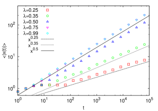
Figure 1: Diffusion. The random walk process (16) is sub-diffusive when $0<\lambda<1/2$, according to $\langle|x(t)|\rangle\sim t^{\nu}$ with $\nu=\lambda$, and is standard diffusive $\langle|x(t)|\rangle\sim t^{1/2}$ when $1/2\leq\lambda<1$.

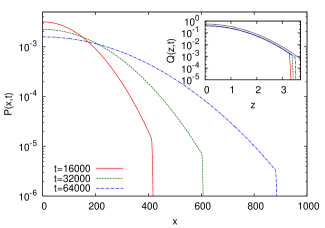
Figure 2: Probability. The right side of the probability distribution $P(x,t)$ of the process (16) is shown for $\lambda=0.55$ and different times. Although the value of $\gamma$ is close to $1/2$ the truncation only involves distribution tails which carry a minimal total probability. Moreover, truncation shifts to the right in time and asymptotically vanishes. This can be better appreciated in the inset where the probability $Q(z,t)$ of $z(t)=x(t)/t^{1/2}$ is shown and compared with a Gaussian (dotted black line).

This process is confined in a box by two reflecting boundaries situated in $L$ and $-L$ where $L=t^{\lambda}$.

If $0<\lambda<1/2$ the process is sub-diffusive according to $\langle|x(t)|\rangle\sim t^{\nu}$ with $\nu=\lambda$, as shown in Fig. 1. Notice that in this case the distribution of $z(t)=x(t)/t^{\nu}$ is approximately uniform between -1 and 1 (for large times) as the box dimension increases slowly with respect to the relaxation of the process in the box.

On the contrary, if $1/2\leq\lambda\leq 1$ the process behaves as an ordinary diffusion with $\langle|x(t)|\rangle\sim t^{1/2}$ so that $\nu=1/2\neq\lambda$, as shown in Fig. 1. In this ordinary diffusive region the effect of the reflecting boundaries is just to kill the tails of the process for $|x|>t^{\lambda}$. The distribution of $z(t)=x(t)/t^{1/2}$, as time $t$ increases, becomes closer to a Gaussian, with the truncation which shifts on the extremes and disappears for large times $t\to\infty$. This is shown in Fig. 2.

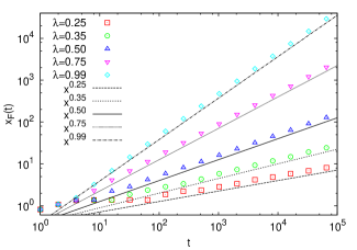
Figure 3: Reaction. Front position $x_{F}$ for different values of $\lambda$ and $\tau=1$ is shown. In all cases $x_{F}(t)\sim t^{\delta}$ with $\delta=\lambda$.

Model (16) is a simplified version of the non Markovian random walk introduced in Ref.s serva2013 ; serva2014 . The stochastic process (16) is a Markovian process so we can use Eq.(2) to describe reaction-diffusion dynamics.

When a reaction term is involved, it turns out that in all cases the exponent $\delta$ of the propagating front equals the exponent $\lambda$ which defines the process, i.e. $x_{F}(t)\sim t^{\delta}$ with $\delta=\lambda$. Therefore, not only the scaling behavior of the front is anomalous in case of sub-diffusion (for $0<\lambda<1/2)$, but also in case of regular diffusion (for $1/2\leq\lambda<1)$. In fact, e.g. in the last case, Eq. (4) reads:

$$\theta(x,t)\sim e^{-x^{2}/4Dt}\Theta(t^{\delta}-|x|)e^{t/\tau}\,,$$ (17)

where $\Theta(x)$ is the Heaviside step function representing the truncation of the distribution tails. Since the truncation overcomes the linear propagation due to the Gaussian diffusion together with the exponential growing of the reaction, one has $x_{F}(t)\sim t^{\delta}$, as can be appreciated in Fig. 3 where the front position $x_{F}(t)=\min\{\,|x|\,;\,\theta(x,t)<0.5\}$ is shown. However, completely equivalent results is obtained by computing the average position of reaction products or their total quantity.

IV The role of tails in a model with subdiffusion

We now consider a more complex model that includes the previously neglected tails, in order to investigate their effect on propagation. We consider

$$x(t+1)=x(t)+\sigma(t),$$ (18)

with $\sigma(t)$ given by

• $\sigma(t)={\rm sign}(x(t))$ with probability $p(x(t),t)$ and

• $\sigma(t)=-{\rm sign}(x(t))$ with probability $1-p(x(t),t)$;

where

$$p(x,t)=\frac{1}{2+\left(\frac{|x|}{t^{\lambda}}\right)^{\eta}}.$$ (19)

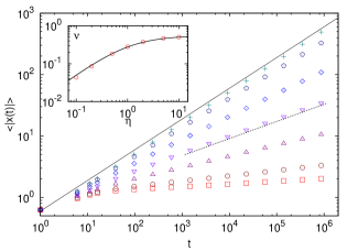
Figure 4: Diffusion. The average $\langle|x(t)|\rangle$ is shown for $\lambda=0.55$ for different values of $\eta$ (from top to bottom $\eta=10\,\,(+)$, $\eta=5.0\,\,(\pentagon)$, $\eta=2.0\,\,(\diamond)$, $\eta=1.0\,\,(\bigtriangledown)$, $\eta=0.5\,\,(\bigtriangleup)$, $\eta=0.2\,\,(\circ)$, $\eta=0.1\,\,(\Box)$). The dashed line is the scaling behavior $\langle|x(t)|\rangle\sim t^{\nu}$ for $\eta=1$, with $\nu$ given by Eq. (22). In the inset the measured scaling $\nu$ is reported ($\circ$) together with the prediction (22) (solid line) at varying $\eta$.

The above model has been motivated by ecological problems. For instance the problem of foraging strategies, with the walker (animal) changing its attitude when it is at the frontier of unexplored regions serva2013 ; serva2014 .

Such a process does not present sharp boundaries. In fact, if $\eta$ is finite, the walker can cross the position $|x|=t^{\lambda}$ but she advances with an increasing difficulty when she is at a larger distance from the origin. However, in the limit $\eta\to\infty$, this model coincides with the model of Section III (which has boundaries in $|x|=t^{\lambda}$). In the opposite case, i.e. for $\eta\to 0$, it is worth noting that the process becomes an “asymmetrical” random walk with probabilities $1/3$ for $\sigma(t)={\rm sign}(x(t))$ and $2/3$ for $\sigma(t)=-{\rm sign}(x(t))$ (in the origin the probability is symmetrical). In this case the walker does not diffuse anymore and the stationary probability $P(x)$ can be easily computed from detailed balance finding $P(x)=\frac{1}{3}\,2^{-|x|}$.
The average $\langle|x(t)|\rangle$ is shown in Fig. 4 for $\lambda=0.55$ and different values of $\eta$. As a consequence of the previous discussion for $\eta$ small the diffusion decline (and for $\eta\to 0$ the diffusion is absent, with $\langle|x(t)|\rangle=$ const.) while for $\eta$ large the process tends to standard diffusion ($\langle|x(t)|\rangle\sim t^{1/2}$ since $\lambda\geq 1/2$). For intermediate values of $\eta$, the process is always subdiffusive. A simple argument to compute the anomalous exponent is as follows. Using Eq. (18) and writing $\langle x(t)\sigma(t)\rangle$ in terms of the conditional expected value with respect to the probability (19) one obtains the exact evolution rule for $\langle x^{2}(t)\rangle$

$$\langle x^{2}(t+1)\rangle-\langle x^{2}(t)\rangle=1-\left\langle\frac{2|x(t)|\left(\frac{|x(t)|}{t^{\lambda}}\right)^{\eta}}{2+\left(\frac{|x(t)|}{t^{\lambda}}\right)^{\eta}}\right\rangle$$ (20)

First of all we assume a diffusive dynamics, $\langle|x(t)|\rangle\sim t^{\nu}$, with monofractal properties, i.e.

$$\langle|x(t)|^{\eta}\rangle\sim\langle|x(t)|\rangle^{\eta}\sim t^{\nu\eta}\,.$$

Such a conjecture has been checked a posteriori. We observe that forcely $\nu<\lambda$, because in the opposite case the r.h.s. of Eq. (20) becomes negative, leading to a non-diffusive dynamics. Therefore one can safely conclude that $\left(|x(t)|/t^{\lambda}\right)^{\eta}$ is vanishing for large times, and Eq. (20) can be approximated by

$$\langle x^{2}(t+1)\rangle-\langle x^{2}(t)\rangle\sim 1-\frac{1}{t^{\lambda\eta}}\langle|x(t)|^{\eta+1}\rangle\,.$$ (21)

The above expression can be analyzed considering three different cases:

$\nu>\lambda\eta/(1+\eta)$

: the second term of equation (21) is negative implying absence of diffusion and contradicting the above assumptions.

$\nu=\lambda\eta/(1+\eta)$

: equation (21) is coherent as far as $\lambda\eta/(1+\eta)\leq 1/2$, since the maximum scaling exponent consistent with equation (21) is $\nu=1/2$.

$\nu<\lambda\eta/(1+\eta)$

: in this case the second term of equation (21) is equal to one (for large times) implying $\nu=1/2$.

In conclusion:

$$\nu=\min\left[\frac{1}{2},\;\frac{\lambda\eta}{1+\eta}\right]\,$$ (22)

and, in the case of $0<\lambda\leq 1/2$ one always has $\nu=\lambda\eta/(1+\eta)$. Notice that, for any $0<\lambda\leq 1$ and in the limit $\eta\to\infty$, one recovers the result already found for the model with sharp boundaries. In the inset of Fig. 4 the perfect agreement of the prediction (22) with the anomalous diffusive exponent $\langle|x(t)|\rangle\sim t^{\nu}$ is shown.

For the understanding of the features of front propagation we have to determine the shape of the probability distribution, $P(x,t)$, of the process (18). Accordingly to the definition of the process we have the following conditional expectation with respect to $x(t)=x$:

$$\langle\sigma(t)|x\rangle=-{\rm sign}(x)\frac{\left(\frac{|x|}{t^{\lambda}}\right)^{\eta}}{2+\left(\frac{|x|}{t^{\lambda}}\right)^{\eta}}.$$ (23)

Let us use the standard procedure to continuously approximate the forward Kolmogorov equation (Fokker-Planck equation in the terminology used in physics) for the probability density $P=P(x,t)$ as

$$\frac{\partial P}{\partial t}=-\frac{\partial(bP)}{\partial x}+\frac{1}{2}\frac{\partial^{2}(aP)}{\partial x^{2}}$$ (24)

where

$$b(x,t)=\langle\sigma(t)|x\rangle=-{\rm sign}(x)\frac{\left(\frac{|x|}{t^{\lambda}}\right)^{\eta}}{2+\left(\frac{|x|}{t^{\lambda}}\right)^{\eta}}.$$ (25)

and

$$a(x,t)=\langle\sigma^{2}(t)|x\rangle-\langle\sigma(t)|x\rangle^{2}=1-b^{2}(x,t).$$ (26)

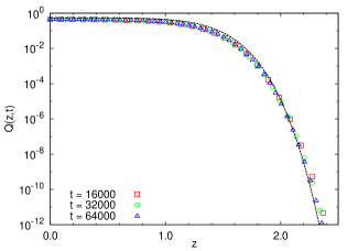
Figure 5: Probability. The right side of the probability distribution $P(x,t)$ of the diffusive process (18) is shown using the rescaled variable $z(t)=x(t)/t^{\nu}$ with $\nu$ given by Eq. (22) for $\lambda=0.55$ and $\eta=5.0$ at different times. The dashed line is the rescaled distribution $Q(z)=\exp(-z^{\eta+1}/(\eta+1))$ as from Eq. (30).

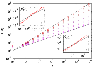
Figure 6: Reaction. Front position for $\lambda=0.55$, with reaction parameter $\tau=1$ and different values of $\eta$ (from bottom to top, $\eta=10\,\,(+)$, $\eta=5.0\,\,(\pentagon)$, $\eta=2.0\,\,(\diamond)$, $\eta=1.0\,\,(\bigtriangledown)$, $\eta=0.5\,\,(\bigtriangleup)$, $\eta=0.2\,\,(\circ)$, $\eta=0.1\,\,(\Box)$) is shown. In all cases the scaling is $x_{F}(t)\sim t^{\delta}$ with $\delta=\lambda=0.55$ (solid line) but there is a transient in which a different exponent (see Eq. (31)) is selected. In the limit case $\eta\to 0$ a linear front behavior ($x_{F}(t)\sim t$ dashed line) is restored. In the inset the scaling behavior in the transient region $x_{F}(t)=(1+\eta)^{1/(1+\eta)}t^{\delta}$ with $\delta$ given by Eq. (31) (dashed line) is shown together with the asymptotic behavior $x_{F}(t)=(A)^{1/\eta}t^{\lambda}$, with $A=8$ corresponding to a threshold $1/10$ for the jump probability (19) (solid line) for $\eta=1.0$ (top left) and for $\eta=2.0$ (bottom right). The matching between the two scalings gives the crossover time (see Eq. (32)).

Moreover, with the change of variable $y=x/t^{\nu}$ one can define the probability density for $y$ as $\tilde{P}(y,t)dy=P(y\,t^{\nu},t)dx$. Since $dx=t^{\nu}\,dy$, one has $\tilde{P}(y,t)=P(y\,t^{\nu},t)t^{\nu}$. This density satisfies the following equation:

$$\frac{\partial\tilde{P}}{\partial t}=\frac{\nu}{t}\frac{\partial(y\tilde{P})}{\partial y}-\frac{1}{t^{\nu}}\frac{\partial(\tilde{b}\tilde{P})}{\partial y}+\frac{1}{2t^{2\nu}}\frac{\partial^{2}(\tilde{a}\tilde{P})}{\partial y^{2}}$$ (27)

where $\tilde{a}(y,t)=a(y\,t^{\nu},t)$ and $\tilde{b}(y,t)=b(y\,t^{\nu},t)$.

First we assume that $\lambda\eta/(1+\eta)>1/2$ which implies $\nu=1/2$ and consider the above equation with $a$ and $b$ given by (26) and (25) with the choice $\nu=1/2$. Neglecting all terms in Eq. (27) which are of higher order than $1/t$ one obtains

$$\frac{\partial\tilde{P}}{\partial t}=\frac{1}{2t}\left(\frac{\partial(y\tilde{P})}{\partial y}+\frac{\partial^{2}(\tilde{P})}{\partial y^{2}}\right)\,.$$ (28)

This equation has a stationary solution $\tilde{P}=\frac{1}{\sqrt{2\pi}}e^{-\frac{y^{2}}{2}}$ which implies that the core of the distribution $P(x,t)$ is Gaussian, $P(x,t)=\frac{1}{\sqrt{2\pi\,t}}\,e^{-\frac{x^{2}}{2t}}$.

Second we assume that $\frac{\lambda\eta}{1+\eta}<1/2$ which implies $\nu=\frac{\lambda\eta}{1+\eta}$. Neglecting all terms in Eq. (27) which are of higher order than $1/t^{2\nu}$ one obtains

$$\frac{\partial\tilde{P}}{\partial t}=\frac{1}{2t^{2\nu}}\left({\rm sign}(y)\frac{\partial(|y|^{\eta}\tilde{P})}{\partial y}+\frac{\partial^{2}(\tilde{P})}{\partial y^{2}}\right)$$ (29)

Also this equation has a stationary solution $\tilde{P}=ce^{-\frac{|y|^{\eta+1}}{\eta+1}}$ where $c=(\eta+1)^{\eta/(\eta+1)}/2\Gamma(1/(\eta+1))$, being $\Gamma(\cdot)$ the gamma function. This implies that the core of the distribution $P(x,t)$ is

$$P(x,t)=\frac{c}{t^{\nu}}\,e^{-\frac{1}{\eta+1}\left|\frac{x}{t^{\nu}}\right|^{\eta+1}}\,.$$ (30)

In conclusion for large times, the distribution approaches a Gaussian when $\lambda\eta/(1+\eta)>1/2$ and $\nu=1/2$, and approaches the above anomalous density when $\nu=\lambda\eta/(1+\eta)<1/2$. Let us remark that the transition between these two densities at $\lambda\eta/(1+\eta)=1/2$ is discontinuous, unless $\eta=1$.

In Fig. 5 we show the rescaled probability distribution associate to the process (18) for $\lambda=0.55$ $\eta=5.0$ and different times together with the prediction of Eq. (30). The agreement is very good.

Let us remark that in the $\eta\to\infty$ limit we obtain the same results already discussed in section III for the model with truncated tails. In particular for $\lambda<1/2$ one has that the anomalous distribution (30) is constant in the interval $-t^{\nu}\leq x\leq t^{\nu}$ and vanishes elsewhere, while for $\lambda>1/2$ the core of the distribution is Gaussian. The effect on tails when $\eta=\infty$ is simply a sharp cut at $|x|=t^{\lambda}$ which obviously disappears when time diverges.

Finally, in the limit $\eta\to 0$, the density (30) is independent from time with value $P(x,t)\sim e^{-|x|}$, confirming what obtained directly choosing $\eta=0$. Nevertheless, the exponential decay is different, considering that for $\eta=0$ we found $P(x,t)\sim 2^{-|x|}$. This difference is a consequence of the fact that the large time limit and the vanishing $\eta$ limit cannot be interchanged as it can be easily checked.

Now we are ready to discuss the front propagation behavior when a reaction term is involved. The argument in Eq.s (4), (9) and (10) would give $x_{F}\simeq\sqrt{2}\,t$ in the Gaussian case (i.e., when $\lambda\eta/(1+\eta)>1/2$) and $x_{F}\simeq(1+\eta)^{1/(1+\eta)}\,t^{\delta}$ with

$$\delta=\frac{1+\lambda\eta}{1+\eta}\,.$$ (31)

for distribution (30) (i.e., when $\lambda\eta/(1+\eta)<1/2$). These two scalings can be observed only for a transient time since, as we will discuss below, the correct asymptotic scaling is $x_{F}(t)\sim t^{\lambda}$, as shown in Fig. 6 where the front position is shown for $\lambda=0.55$, with reaction parameter $\tau=1$ and different values of $\eta$. In all cases the asymptotic scaling is $x_{F}(t)\sim t^{\delta}$ with $\delta=\lambda=0.55$, but there is a transient in which the exponent is given by Eq. (31). In the inset it is clearly shown for $\eta=1$ the preasymptotic and asymptotic behavior of the front position.

A simple theoretical explanation to justify the behavior of the asymptotic front properties goes as follows. Let us first remark that the forward jump probability (19) when $|x|$ is of the order of $t^{\lambda+\epsilon}$ vanishes as $t^{-\epsilon\eta}$, therefore, for large times the support of the distribution $P(x,t)$ vanishes when $|x|\sim t^{\lambda+\epsilon}$. This implies that the front $x_{F}(t)$ cannot move faster then $x_{F}(t)\sim t^{\lambda}$ when $t$ is large. On the other hand, when $|x|\sim t^{\lambda-\epsilon}$, the forward jump probability (19) tends to $1/2$ for large times for any positive $\epsilon$, this implies that the front $x_{F}(t)$ moves at least as fast as $x_{F}(t)\sim t^{\lambda}$ when $t$ is large. In conclusion, $x_{F}(t)\sim t^{\lambda}$.

A rough determination of the crossover time, i.e. the time at which the front propagation starts to reach its asymptotic behaviour, can be given with a matching between the position of the front in the preasymptotic regime, $x_{F}(t)\simeq(1+\eta)^{1/(1+\eta)}t^{\delta}$, and the value $\tilde{x}(t)$ at which the jump probability (19) is small, $p(\tilde{x},t)=1/(2+(|\tilde{x}|/t^{\lambda})^{\eta})=1/(2+A)\ll 1$, i.e. when $\tilde{x}(t)\simeq A^{1/\eta}t^{\lambda}$, where $A$ is an appropriately large constant. The matching between those behaviours gives

$$t^{*}\simeq\left(\frac{A^{1/\eta}}{(\eta+1)^{(\eta+1)}}\right)^{\frac{(1+\eta)}{(1-\lambda)}}.$$ (32)

With $A=8$, corresponding to a threshold $1/10$ for the jump probability (19), one has a good agreement with the actual results, as shown in the insets of figure 6.

V Conclusions

We study a class of modified random walk processes, whose probability distributions can be analytically determined, which can have, at varying a control parameter, standard or sub-diffusive behavior. For reaction-diffusion systems, with a pulled reaction function, the scaling exponent of the diffusive problem is not relevant for the asymptotic behavior of the front: the basic ingredient to determine the front propagation behavior is the shape of tails of the probability distribution. This holds both for standard and sub-diffusion.

Our results show, as already discussed in Sokolov2006 ; Mendez2009 ; Nepomnyashchy2016 , that the details of the diffusion and reaction dynamics play a fundamental role in determining the front propagation features.

We conclude mentioning some topics which would be interesting to investigate. In our study we use a macroscopic description in terms of concentration, in addition we considered a pulled reaction function which acts even for very small concentration. The macroscopic approach is not appropriate if the density of transported “particles” is not very large and therefore the discrete nature of the population cannot be neglected. We expect that the discreteness of the population will impact in nontrivial ways on the spatial propagation properties of the population. In addition, a topic to investigate, even in the macroscopic approach, is the role of shape of $f(\theta)$. For instance we can probe how the use of reaction term in the class of Allee non linearity (see for example neufeld2010 ) impact on the front propagation behavior.

References

- (1) Z. Neufeld and E. Hernández-García, Chemical and biological processes in fluid flows : a dynamical systems approach, Imperial College Press, London, UK, (2010).
- (2) R. Burioni, and D. Cassi. Random walks on graphs: ideas, techniques and results, Journal of Physics A: 38, R45 (2005).
- (3) R. Metzler, J.H. Jeon, A.G. Cherstvy and E. Barkai, Anomalous diffusion models and their properties: non-stationarity, non-ergodicity, and ageing at the centenary of single particle tracking. Phys. Chem. Chem. Phys. 16, 24128 (2014).
- (4) V. Zaburdaev, S. Denisov, and J. Klafter, Lévy walks. Reviews of Modern Physics 87, 483 (2015).
- (5) R. Mancinelli, D. Vergni and A. Vulpiani, Superfast front propagation in reactive systems with non-Gaussian diffusion, Europhysics Letters 60, 532 (2002).
- (6) R. Mancinelli, D. Vergni and A. Vulpiani, Front propagation in reactive systems with anomalous diffusion. Physica D, 85, 175 (2003).
- (7) R. Burioni, S. Chibbaro, D. Vergni and A. Vulpiani, Reaction spreading on graphs, Physical Review E 86, 055101(R) (2012).
- (8) I.M. Sokolov, M.G.W. Schmidt and F. Sagués, Reaction-subdiffusion equations, Physical Review E 73, 031102 (2006).
- (9) D. Campos and V. Méndez, Nonuniversality and the role of tails in reaction-subdiffusion fronts, Physical Review E 80, 021133 (2009).
- (10) S. Fedotov, Non-Markovian random walks and nonlinear reactions: subdiffusion and propagating fronts, Physical Review E 81, 011117 (2010).
- (11) A.A. Nepomnyashchy and V. A. Volpert, An exactly solvable model of subdiffusion-reaction front propagation. Journal of Physics A: Mathematical and Theoretical 46, 065101 (2013).
- (12) A.A. Nepomnyashchy, Mathematical Modelling of Subdiffusion-reaction Systems. Mathematical Modelling of Natural Phenomena 11.1, 26 (2016).
- (13) M.J. Saxton, A biological interpretation of transient anomalous subdiffusion. I. Qualitative model. Biophysical Journal 92, 1178 (2007).
- (14) M. Freidlin, Functional integration and partial differential equations, (Princeton Univ. Press, Princeton NY 1985).
- (15) G. Gaeta and R. Mancinelli, Asymptotic Scaling in a Model Class of Anomalous Reaction-Diffusion Equations. Journal of Nonlinear Mathematical Physics 12, 550 (2005).
- (16) M.E. Fisher, Shape of a Self-Avoiding Walk or Polymer Chain. J. Chem. Phys. 44, 616 (1966).
- (17) S. Berti, M. Cencini, D. Vergni and A. Vulpiani, Extinction dynamics of a discrete population in an oasis, Physical Review E 92, 012722, (2015).
- (18) M. Serva, Scaling behavior for random walks with memory of the largest distance from the origin, Physical Review E 88, 052141 (2013).
- (19) M. Serva, Asymptotic properties of a bold random walk, Physical Review E 90, 022121 (2014).