On the characterisation of SiPMs from pulse-height spectra

Abstract

Methods are developed, which use the pulse-height spectra of SiPMs measured in the dark and illuminated by pulsed light, to determine the pulse shape, the dark-count rate, the gain, the average number of photons initiating a Geiger discharge, the probabilities for prompt cross-talk and after-pulses, as well as the electronics noise and the gain fluctuations between and in pixels. The entire pulse-height spectra, including the background regions in-between the peaks corresponding to different number of Geiger discharges, are described by single functions. As a demonstration, the model is used to characterise a KETEK SiPM with 4384 pixels of $15\,\upmu$m$\times 15\,\upmu$m area for voltages between 2.5 and 8 V above the breakdown voltage. The results are compared to other methods of characterising SiPMs. Finally, examples are given, how the complete description of the pulse-eight spectra can be used to optimise the operating voltage of SiPMs, and a method for an in-situ calibration and monitoring of SiPMs, suited for large-scale applications, is proposed.

1 Introduction

Silicon photomultipliers (SiPMs), pixel arrays of avalanche photodiodes operated above the breakdown voltage, are becoming the photon detectors of choice for many applications [1, 2, 3]. They are robust, have a high photon-detection efficiency, achieve single-photon detection and resolution, operate at modest voltages, are not affected by magnetic fields, and are relatively inexpensive. Disadvantages are their high dark-count rate at room temperature, which rapidly increases with radiation damage, and the excess noise due to inter-pixel cross-talk and after-pulses.

Various methods have been developed to determine the main SiPM-performance parameters [4, 5, 6, 7, 8, 9]: the photon-detection efficiency (PDE), the gain (Gain), the break-down voltage ($V_{bd}$), the dark-count rate (DCR), and the correlated noise ($CN$). Typically, pulse-height spectra recorded in the dark are used to determine DCR and CN: $DCR=f_{0.5}/t_{gate}$, where $f_{0.5}$ is the fraction of events above one half of the mean pulse-height ($PH$) of a single Geiger discharge and $t_{gate}$ the gate width, and $CN=f_{1.5}/f_{0.5}$, where $f_{1.5}$ is the fraction of events above 1.5 times the $PH$ of a single Geiger discharge. From the $PH$ spectra recorded with light from a pulsed LED or laser, the mean number of photons initiating a Geiger discharge, $N_{\gamma}$, which is proportional to the PDE, the Gain, the electronics noise, $\sigma_{0}$, and the gain differences between the different pixels and within one pixel, $\sigma_{1}$, are obtained. The spectra are analysed by fitting multiple Gauss functions to the individual peaks, ignoring the background events in-between the peaks. The problem of the method is that the fit regions have to be selected and that it is difficult to evaluate the influence of the ignored background on the results. In order to avoid the selection of event regions, methods based on Fourier transforms are also used for the Gain determination. In Refs. [5] and [6] long transient are recorded in the dark and under continuous low-light illumination. Pulses are identified and analysed by software, and a complete characterisation, including signal shape, gain, primary dark-count rate, prompt and delayed cross-talk probability, after-pulse probability and excess noise factor, is achieved.

In this paper, models are developed, which describe the entire PH spectra: The model for the pulsed-light data takes into account the statistics of the photons initiating Geiger discharges, the statistics of prompt cross-talk and the pulse-height distribution and statistics of after-pulses. The model for the data without light takes into account the random arrival times of dark pulses and the effects of prompt cross-talk. By fitting the models to the measurements, a complete SiPM characterisation is achieved.

Finally, the results of the fits are used to determine the voltage for the optimal resolution of the number of photons ($N_{\gamma}$), and to develop a method, which allows to determine Gain and $N_{\gamma}$ in situations in which the peaks corresponding to different numbers of photoelectrons cannot be resolved. The method does not require fits but only uses the SiPM excess-noise factor, and the first and second moments of the measured PH distributions.

2 Sensors investigated and measurements

The SiPMs investigated were fabricated by KETEK [10]. Their number of pixels is $N_{pix}=4384$, and their pitch is $15\,\upmu$m$\times 15\,\upmu$m. Fig. 1 shows a schematic cross section of a single SiPM pixel, which has a high-field charge-amplification region of about $1\,\upmu$m depth. More information on the SiPMs can be found in Refs. [11, 12].

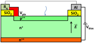
Figure 1: Schematic cross section of a single pixel of the KETEK SiPM.

The measurements were made in a temperature-controlled light-tight box. As light source, a pulsed LED with a wavelength of 470 nm and a pulse width of about 2 ns has been used. The LED was housed outside of the light-tight box, and an optical fiber guided the light to the SiPM. The SiPM was read out via a Philips Scientific Amplifier 6954 [13] by a CAEN QDC V965 [14]. The read-out was AC coupled with a time constant $\tau_{\mathrm{AC}}\approx 5\,\upmu$s. The LED was triggered by a HP 8110A Pulse Pattern Generator [15] by a pulse of 5 ns full width, and a pulse generator from Stanford Research Enterprise [16] provided the 100 ns wide gate for the QDC.

The following measurements were performed at 20^∘C for voltages between 29.5 and 35 V in 0.5 V steps, which is above the breakdown voltage $V_{bd}\approx 27\,$V:

1. Delay curve,

2. Pulse-height (PH) spectra in the dark,

3. $PH$ spectra for low light intensity, corresponding to an average between 0.8 and 1.6 Geiger discharges in the voltage range of the measurements,

4. $PH$ spectra for high light intensity, $\approx 16$ times higher than for low light.

For every PH spectrum $5\times 10^{5}$ events were recorded. The absolute light yield of the LED is not known, however for a given voltage scan it was stable within < 1 %.

3 Data analysis and results

3.1 Delay curve

The delay curves allow to determine the timing of the gate relative to the SiPM pulse, the effective gate width for the pulse-height measurement, $t_{gate}^{eff}$, the decay time constant of the SiPM signal including the effects of after-pulsing, $\tau$, and the time constant of the AC coupling of the readout, $\tau_{AC}$, which is typically used when reading out SiPMs. We call $\langle PH_{meas}(t)\rangle$ the average of the pulse-height spectrum recorded by the QDC for a measurement at a given $t$, which is the time between the start of the SiPM pulse and the start of the integration by the gate. For modeling the delay curve, we consider a SiPM-current pulse $I(t^{\prime})=(Q_{0}/\tau)\cdot e^{-t^{\prime}/\tau}$ for $t^{\prime}>0$ and $I(t^{\prime})=0$ for $t^{\prime}\leq 0$. The integrals over the gate of a pulse starting at time $t$ before the start of the integration, $t<0$, and after the start of the integration, $t>0$, are

$$PH(t)=\left\{\begin{array}[]{ll}Q_{0}\cdot e^{\frac{t}{\tau}}\,\big{(}1-e^{-\frac{t_{gate}}{\tau}}\big{)}&\hbox{\rm{for}\,\, $t<0$,}\\ \vspace{1mm}Q_{0}\cdot\big{(}1-e^{-\frac{t_{gate}-t}{\tau}}\big{)}&\hbox{\rm{for}\,\, $0\leq t<t_{gate},$}\\ 0&\hbox{\rm{for}\,\, $t\geq t_{gate}$.}\end{array}\right.$$ (1)

So far AC coupling has been ignored. In the presence of AC coupling, the following term has to be subtracted from Eq. 1

$$PH_{AC}(t)=\left\{\begin{array}[]{ll}\vspace{1mm}Q_{0}\cdot\Big{(}\frac{e^{\frac{t}{\tau_{AC}}}}{1-\tau/\tau_{AC}}\big{(}1-e^{-\frac{t_{gate}}{\tau_{AC}}}\big{)}-\frac{e^{\frac{t}{\tau}}}{(\tau_{AC}/\tau)-1}\big{(}1-e^{-\frac{t_{gate}}{\tau}}\big{)}\Big{)}&\hbox{\rm{for}\,\, $t<0$,}\\ \vspace{2mm}Q_{0}\cdot\Big{(}\frac{1-e^{-\frac{t_{gate}-t}{\tau_{AC}}}}{1-\tau/\tau_{AC}}-\frac{1-e^{-\frac{t_{gate}-t}{\tau}}}{(\tau_{AC}/\tau)-1}\Big{)}&\hbox{\rm{for}\,\, $0\leq t<t_{gate},$}\\ 0&\hbox{\rm{for}\,\, $t\geq t_{gate}$.}\end{array}\right.$$ (2)

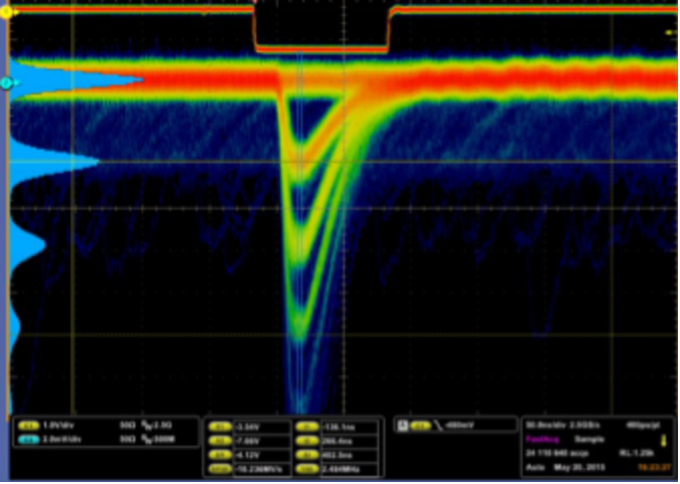
(a)

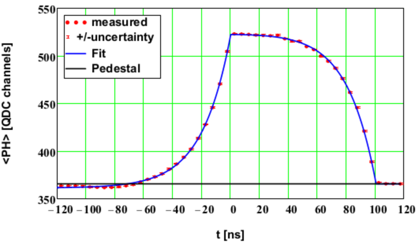
(b)

Figure 2: (a) Screenshot from the oscilloscope for the SiPM operated at 32 V illuminated by the pulsed LED. Top line, the gate, and bottom lines, the SiPM transients, where bands corresponding to 0, 1, 2, 3, and 4 Geiger discharges can be distinguished. (b) Delay curve measured with a pulse-height analyser (CAEN QDC), and the fit described in the text. The line at $PH=365.5$ indicates the pedestal value. If the SiPM pulse precedes the gate (delays < -80 ns), a smaller $PH$ value than the pedestal is observed, which is caused by the AC coupling of the SiPM readout.

Fig. 2a shows a screenshot of the gate and of SiPM pulses recorded at 32 V for a SiPM illuminated by the pulsed LED. Fig. 2b shows the corresponding delay curve, the average $PH$ for the different delay times, $t$, $\langle PH{meas}(t)\rangle$. The data points are represented by symbols and the fit by $PH(t)-PH_{AC}(t)$ by the solid line. The fit, including the AC coupling, provides a good description of the data, which is not the case if the AC coupling is not taken into account. The reason is that the base line is higher, if the SiPM signal occurs after the gate ($t>100$ ns) than if it occurs before the gate ($t<-80$ ns), which is caused by the AC coupling. The horizontal line in Fig. 2b shows the base line for a SiPM signal after the gate.

For a given PH threshold, $PH_{thr}$, we define an effective gate width, $t_{gate}^{eff}$, as the time difference between the two intercepts of the delay curve with the constant $PH_{thr}$. From Eq. 1 follows:

$$t_{gate}^{eff}(PH_{thr})=t_{gate}+\tau\cdot\ln\Big{(}\frac{Q_{0}-PH_{thr}}{PH_{thr}}\big{(}1-e^{-\frac{t_{gate}}{\tau}}\big{)}\Big{)}.$$ (3)

Eq. 3 is used in Sect. 3.3 for determining the dark-count-rate. For the parameters determined by the fit to the data, $t_{gate}=(100.67\pm 0.12)$ ns and $\tau=(19.95\pm 0.14)$ ns, $t_{gate}^{eff}(0.5\cdot Q_{0})=(100.54\pm 0.12)$ ns, thus essentially equal to $t_{gate}$. Only the statistical errors are given, in order to give an idea about the sensitivity of the method. No study of systematics has been made, however it is expected that the systematic uncertainties dominate.

3.2 Pulse-height measurements with a pulsed LED

The PH spectra measured with the SiPM illuminated by a pulsed LED, d$N_{LED}/\mathrm{d}PH$, were recorded at 20^∘C and reverse voltages from 29.5 to 35 V in steps of 0.5 V, which is above the breakdown voltage of about 27 V. The results are shown in Fig. 3. The peaks corresponding to 0, 1, and more Geiger discharges are well separated. We follow the usual convention and use the symbol npe, the abbreviation of number-of-photoelectrons, for the number of Geiger discharges. The linear increase of $Gain$ with voltage is evident from the increase of the distance between the peaks. The increase of the photon-detection efficiency, PDE, with increasing voltage is seen as a decrease of the fraction of events in the $npe=0$ peak and an increase of the fraction of events in the $npe\geq 1$ peaks. The increase of the widths of the $npe$ peaks with voltage is due to the increase of the dark-count rate, which via the AC coupling causes additional fluctuation of the baseline.

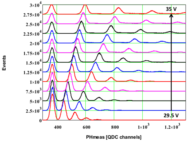
Figure 3: Pulse-height spectra for voltages from 29.5 to 35 V in steps of 0.5 V illuminated by a pulsed LED. For clarity the data points are shifted vertically in steps of 2500 for increasing voltages. Each data set consists of $5\times 10^{5}$ events.

From the $PH$ spectra the voltage dependence of the following SiPM parameters can be obtained: the $Gain$ from the distance between the $npe$ peaks, the average number of photons initiating a Geiger discharge $\langle N_{\gamma}\rangle\equiv\mu=-\ln(f_{0})$, where $f_{0}$ is the fraction of events in the pedestal peak corrected for dark pulses, the standard deviation of the electronics noise, $\sigma_{0}$, from the width of the $npe=0$ peak, and the contribution from the gain spread between and in the individual pixels, $\sigma_{1}$, from the variances of the $npe=i$ peaks using $\sigma_{i}^{2}=\sigma_{0}^{2}+i\cdot\sigma_{1}^{2}$. In addition, the pulse-height spectra are sensitive to prompt and delayed cross-talk and after-pulsing. As the LED light intensity is constant during the voltage scan, $PDE(V)\propto\ \mu(V)$, were PDE is the photon-detection efficiency at the wavelength of the LED light.

The standard method of analysing the pulse-height spectra is to fit Gauss functions to the individual $npe$ peaks and derive the quantities discussed above from the positions, widths and number of events in the peaks [4, 8]. For the $Gain$ determination, also a Fourier-transform method is frequently used. The advantages of these methods is that they are in principle straight-forward. However, as seen in Fig. 4, there is a significant number of events in-between the $npe$ peaks, which cannot be described by the Gauss functions. Therefore, the regions of the fits have to be selected and it is difficult to estimate how much the parameters extracted are affected. In addition, it is not clear if the background in-between the peaks should be subtracted or not. We therefore propose a method, which describes the entire PH spectrum with a single function.

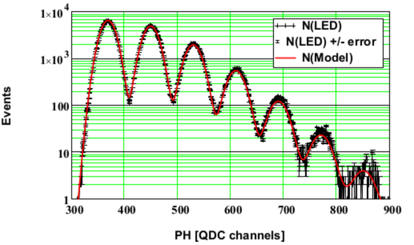
(a)

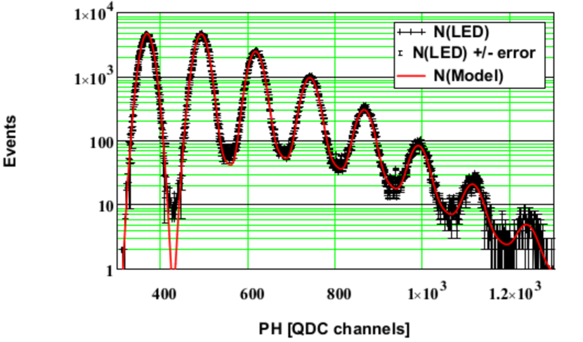
(b)

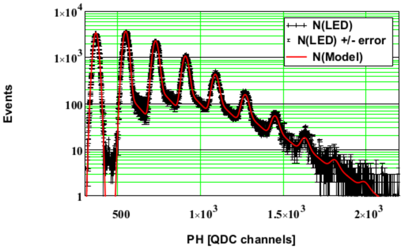
(c)

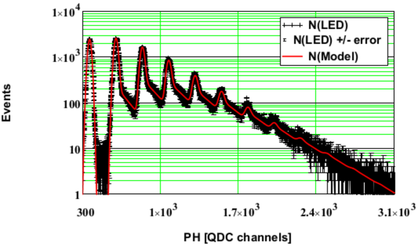
(d)

Figure 4: Pulse-height spectra in logarithmic scale for the SiPM illuminated by a pulsed LED at (a) 29.5 V, (b) 31 V, (c) 33 V, and 35 V. The points with error bars are the data, and the solid lines the fits described in the text.

We assume that the number of photons initiating a Geiger discharge follows a Poisson distribution with the mean $\mu$. Each Geiger discharge can produce secondary Geiger discharges, either prompt or delayed. For the prompt cross-talk we assume a Borel distribution with parameter $\lambda$, which results in a Generalized Poisson (GP) distribution for $k$ discharges [17, 18]

$$GP_{k,\mu,\lambda}=\frac{\mu\cdot(\mu+k\cdot\lambda)^{k-1}\cdot e^{-(\mu+k\cdot\lambda)}}{k!}.$$ (4)

The Borel-branching parameter is denoted $\lambda$ and the probability that a single Geiger discharge produces one or more prompt cross-talk pulses is $1-\exp(-\lambda)$. The mean value of the $GP$ distribution is $\mu/(1-\lambda)$ and its variance $\mu/(1-\lambda)^{3}$. We are aware that prompt cross-talk is essentially limited to the neighbours of the discharging pixel, and $GP$ overestimates the additional number of discharging pixels. However, as long as $\lambda\lesssim 0.25$, the effect is negligible. This has been checked by making the analysis assuming a branching process to the four closest neighbours only.

Inspecting Fig. 4, which displays the pulse-height spectra measured at 29.5, 31, 33 and 35 V in logarithmic scale, one notices that with increasing voltage a significant number of events appear in-between the $npe$ peaks for $npe\geq 1$. We attribute them to delayed cross-talk and after-pulsing, named $AP$ in the following. From the events between the $npe=1$ and $npe=2$ peaks, which correspond to single-$AP$ events, we conclude that their probability distribution can be approximately described by an exponential

$$\frac{\mathrm{d}p_{1,1}}{\mathrm{d}PH}=(1/\beta)\cdot e^{-(PH-PH_{1})/\beta}\,\,\mathrm{for}\,PH\geq PH_{1},$$ (5)

with the exponential slope $\beta$, and the mean pulse-height of the $npe=1$ peak $PH_{1}$. Here, and in the following, the first index, $k$, refers to the number of prompt discharges, and the second, $i$, to the number of $AP$ discharges.

A side remark: We did not expect an exponential distribution, and actually observe different distributions for other types of SiPMs. For a further discussion we refer to Appendix A.

If there are $i>1\,AP$ discharges in an event, which can occur for $k\geq 2$ prompt Geiger discharges, the probability distributions are given by the convolution of $i$ exponentials

$$\frac{\mathrm{d}p_{k,i}}{\mathrm{d}PH}=\frac{(PH-PH_{k})^{i-1}}{(i-1)!\cdot\beta^{i}}\,e^{-(PH-PH_{k})/\beta}\,\,\mathrm{for}\,PH\geq PH_{k},$$ (6)

where $PH_{k}=Ped+k\cdot Gain$ is the mean PH of the $npe=k$ peak. The mean pulse-height of the pedestal peak is denoted by $Ped\equiv PH_{0}$, and the distance between the $npe$ peaks by $Gain$. For the probability distribution that $k$ prompt discharges produce $i\,AP$ discharges, the binomial distribution is assumed

$$B_{k,i,\alpha}=\binom{k}{i}\alpha^{i}(1-\alpha)^{k-i},$$ (7)

with the probability $\alpha$ that a Geiger discharge also causes an AP discharge. Here a binomial distribution is assumed, as a significant fraction of the AP discharges is expected in the same pixel in which the primary discharge has occurred. Eq. 7 ignores the possibility of more than one AP discharge in the same pixel. This however is a small effect, if the $AP$ probability does not exceed $\approx 25$ %. For the prompt Geiger discharges, the noise due to electronics and differences in $Gain$ are taken into account by Gauss functions with variances $\sigma_{k}^{2}=\sigma_{0}^{2}+k\cdot\sigma_{1}^{2}$. For the smearing of the single-$AP$ exponential from the $npe=k$ peak the approximate formula

$$\frac{\mathrm{d}p_{k,1}}{\mathrm{d}PH}=\frac{e^{-(PH-PH_{k})/\beta}}{\sqrt{2\,\pi}\cdot\sigma_{k}\cdot\beta}\int\limits_{-\infty}^{PH}\,e^{-\frac{(PH^{\prime}-PH_{k})^{2}}{2\,\sigma_{k}^{2}}}\,\mathrm{d}PH^{\prime}$$ (8)

is used, which agrees with the exact convolution to within 1 % as long as $\sigma_{k}/\beta<0.2$. The distribution of $i\geq 2$ convoluted exponentials is sufficiently smooth, so that no smearing is necessary and Eq. 6 can be used. Thus the complete probability density distribution reads:

$$\frac{\mathrm{d}p}{\mathrm{d}PH}=\left\{\begin{array}[]{ll}\Big{[}GP_{0,\mu,\lambda}\cdot Gauss(PH;0,\sigma_{0})\,+\\ \sum_{k=1}^{k_{max}}\Big{(}GP_{k,\mu,\lambda}\cdot\big{(}B_{k,0,\alpha}\cdot Gauss(PH;k,\sigma_{k})\,+\\ B_{k,1,\alpha}\cdot\frac{\mathrm{d}p_{k,1}(PH)}{\mathrm{d}PH}+\sum_{i=2}^{k}B_{k,i,\alpha}\cdot\frac{\mathrm{d}p_{k,i}(PH)}{\mathrm{d}PH}\big{)}\Big{)}\,\Big{]},\end{array}\right.$$ (9)

with

$$Gauss(PH;k,\sigma_{k})=\frac{1}{\sqrt{2\,\pi}\,\sigma_{k}}\cdot e^{-\frac{PH-(Ped+k\cdot Gain)}{2\,\sigma_{k}^{2}}}.$$ (10)

This probability density distribution, multiplied with the normalisation constant, Norm, is fitted to the $PH$ spectra to determine the best estimate of the 9 parameters: the normalisation Norm, the mean number of photons initiating a Geiger discharge $\mu$, the branching probability for prompt cross talk $\lambda$, the after-pulsing probability $\alpha$, the inverse of the exponential slope of the after-pulse PH distribution $\beta$, as well as Ped, Gain, $\sigma_{0}$, and $\sigma_{1}$. The value of $k_{max}$ for the fit of the low-light data is set to 8.

The results of the fits, evaluated for $k_{max}=15$, are shown as solid lines in Fig. 4 for the data at 29.5, 31, 33, and 35 V. The description of the data is satisfactory, with $\chi^{2}/NDF$ values between 1.0 and 1.8 for numbers of degrees of freedom, NDF, between 460 and 1600.

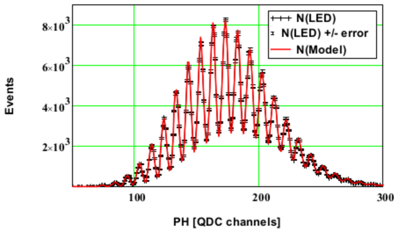
(a)

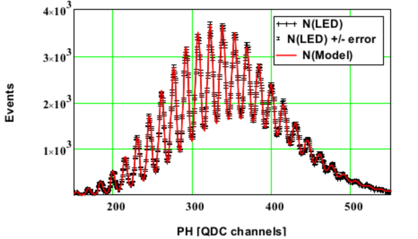
(b)

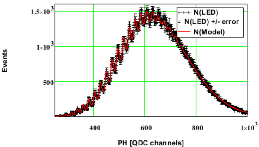
(c)

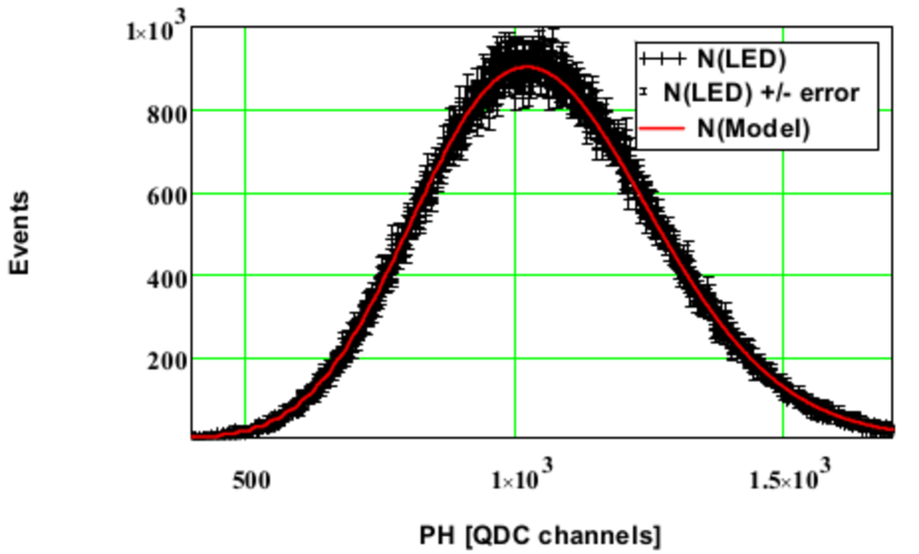
(d)

Figure 5: Pulse-height spectra for the SiPM illuminated by the pulsed LED for a 16 times higher light intensity compared to the data shown in Fig. 4 at (a) 29.5 V, (b) 31 V, (c) 33 V, and 35 V. The points with error bars are the data, and the solid lines the results of the model calculations using Eq. 9 with the SiPM parameters determined from the fits for low light intensities and $k_{max}=50$.

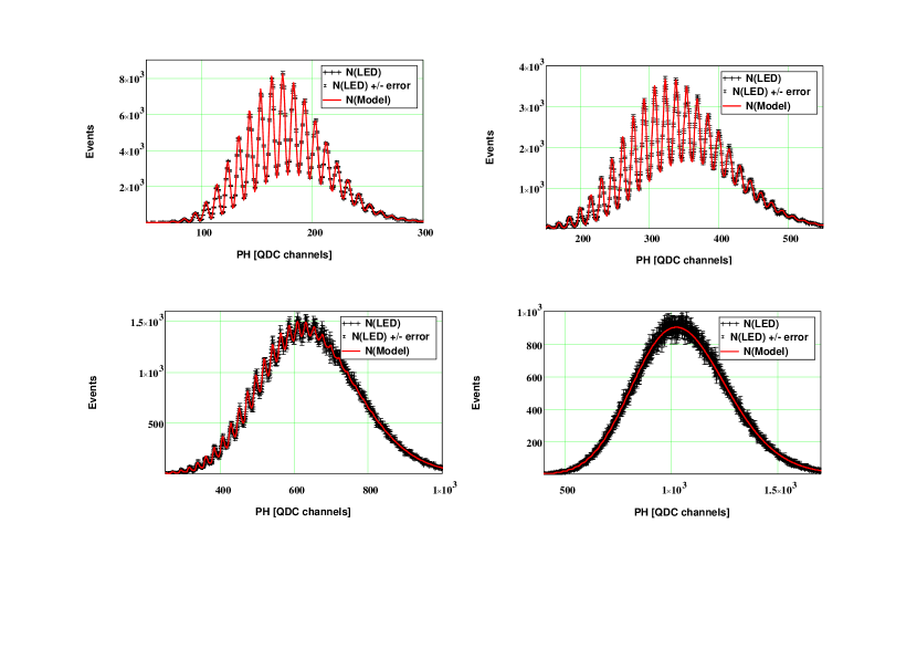
Figure 6: Expanded view of the pulse-height spectrum for the SiPM at 31 V already shown in Fig. 5b, which demonstrates the quality of the prediction using the results from the fit to the data with low-light intensity. Arrows indicate the pedestal, $npe=0$, the average number of photoelectrons, $npe=\mu=18.55$, and the peaks corresponding to $npe=6$, 23 and 33.

In addition, data with an approximately 16 times higher LED intensity have been taken. To avoid saturation the low-gain QDC channel, with an $\approx 1/8$ lower gain, has been used. One aim of these measurements was to verify, if the parameters determined from the low-light data can be used to predict the SiPM response for higher light intensities. Fig. 5 shows the comparison of the prediction with the data for the voltages of 29.5, 31, 33, and 35 V. The agreement is excellent. This can be better judged from Fig. 6, which shows as an example the 31 V data with an expanded scale. Arrows indicate the positions of $npe=0$ (pedestal), 6, 23 and 33. For the prediction, the values of Norm is adjusted for every voltage. The values differ by up to 1 % from the number of entries. The reason is that in the comparison of the data with the model prediction, the value of the function and not the integral over the bin is used, which causes small differences. The values of $\lambda$ and $\alpha$ are taken from the low-light fit. To account for the increased light intensity, the low-light value of $\mu$ is multiplied by the voltage-independent factor 16.275, which results in the best description of the data. The value for the 31 V data, $\mu=18.55$, is marked by an arrow in Fig. 6. To account for the reduced QDC gain, the low-light Gain value is multiplied by 1/7.85, again determined from the model-to-data comparison. For the evaluation of Eq. 9 $k_{max}=50$ is used.

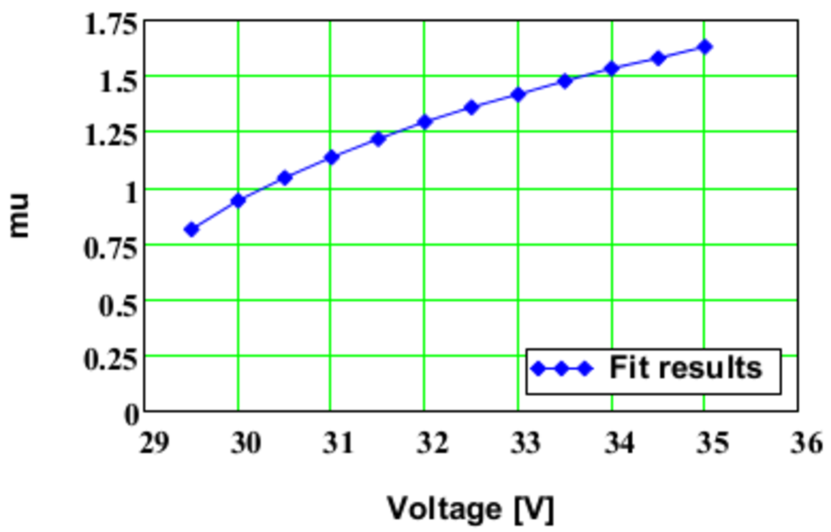
(a)

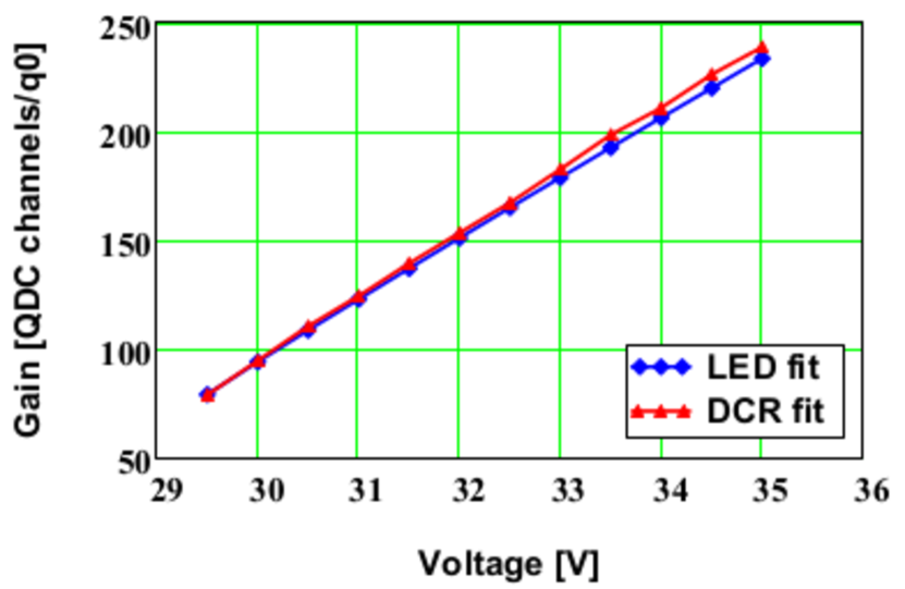
(b)

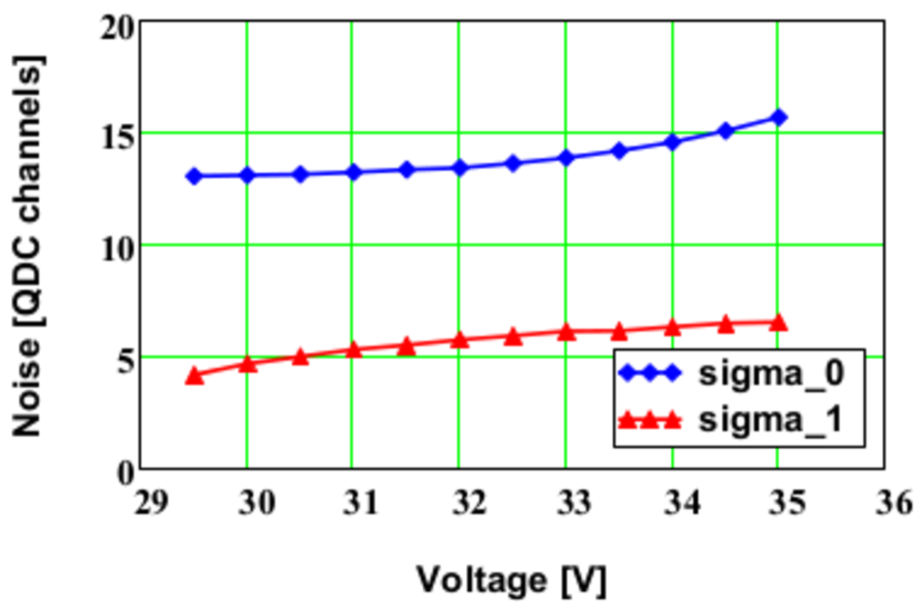
(c)

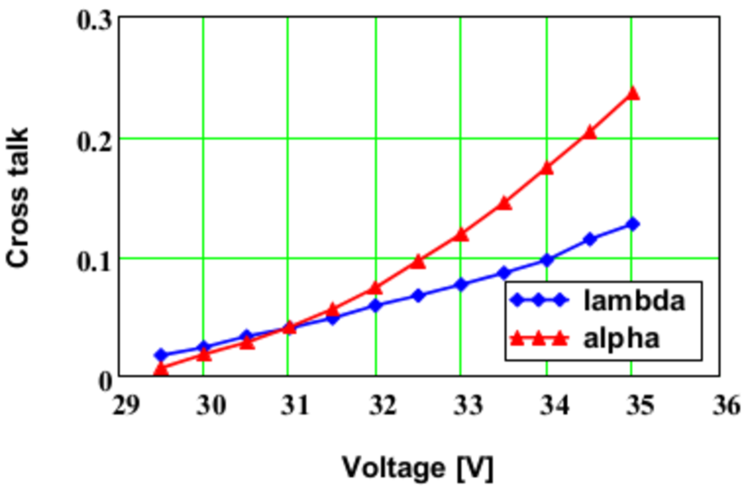
(d)

Figure 7: Voltage dependence of (a) $\mu$ from the low-light fits, (b) Gain in units of QDC channels over elementary charge $q_{0}$ from the low-light fits and the DCR fits presented in Sect. 3.3, and (c) $\sigma_{0}$, $\sigma_{1}$ and (d) $\alpha$ and $\lambda$ from the low-light fits.

Fig. 7 shows the voltage dependence of $\mu$, Gain, $\sigma_{0}$, $\sigma_{1}$, $\alpha$ and $\lambda$ for the fits to the low-light data. The statistical errors from the fits are smaller than the size of the dots. The increase with voltage of $\mu$ reflects the increase of the photon-detection efficiency at the wavelength of the LED light of 470 nm. As expected, the gain increases linearly with voltage with a slope of $\mathrm{d}Gain/\mathrm{d}V=28.01\pm 0.05$  QDC channnels/V, and an intercept of $V_{to}=26.638\pm 0.020$ V, the voltage, at which the Geiger discharges turns off. We note that for the SiPM studied, the breakdown voltage determined from the current-voltage characteristics is about 1 V above $V_{to}$ [11]. The width of the pedestal peak, $\sigma_{0}$ is constant up to 32.5 V, and then shows a small increase, which is caused by the increase in dark-count rate and Gain, and the AC coupling of the readout. The value of $\sigma_{1}$, which describes the variations of Gain between pixels and within pixels, also shows a small increase. As $Gain=\mathrm{d}Gain/\mathrm{d}V\cdot(V-V_{to})\propto C_{pix}\cdot(V-V_{to})$, $\sigma_{1}$ has one contribution $\sigma_{1}^{(1)}=(V-V_{to})\cdot\delta C_{pix}$ from the variation of the pixel capacitance, $\delta C_{pix}$, and a second contribution $\sigma_{1}^{(2)}=\mathrm{d}Gain/\mathrm{d}V\cdot\delta V_{to}$ from the variation of the threshold voltage, $\delta V_{to}$. The term $\delta C_{pix}$ is expected not to depend on V, and from the weak voltage dependence of $\sigma_{1}$ we can exclude a significant contribution from the first term, which is $\propto(V-V_{to})$. We conclude that the second term, $\sigma_{1}^{(2)}$, dominates, and, using the value of $\mathrm{d}Gain/\mathrm{d}V$ from Fig. 7b, we find that $\delta V_{to}$ changes from 150 mV at 29.5 V to 230 mV at 35 V. Finally, Fig. 7 d shows the voltage dependence of the prompt-cross-talk probability, $\lambda$ and the after-pulse probability $\alpha$. As expected, they both increase with voltage.

To summarise: The model developed provides with a single function a precise description of the entire SiPM pulse-height spectra for pulsed light. Both low-light and high-light data are described with the same SiPM parameters, which is a significant test of the model. From the correct description of the intensities of the npe peaks, we conclude that the Borel-branching process for the prompt cross-talk, which results in a Generalised Poisson distribution of the number of prompt Geiger discharges, is a valid assumption. This conclusion has already been reached in Ref. [18]. From the correct description of the smooth background, we conclude that the assumed exponential pulse-height distribution and the binomial-branching process for the after-pulses are also valid. We expect that the pulse-height distribution for after-pulses will be different for different SiPM designs, and thus has to be determined for each case. An example of a possible parametrisation is derived in Appendix A.

Compared to previous methods, the entire pulse-height spectra are fitted by a single function and no bin selection is required. This significantly eases a reliable and fully automatic SiPM characterisation. In Sect. 4 the complete description of the pulse-height spectra will be used to determine the optimal SiPM-operating conditions and develop and test a new method to determine $\mu$ and Gain, when the npe peaks can not be separated for the Gain determination and the methods available so far fail.

3.3 Pulse-height measurement without illumination

Pulse-height spectra measured without illumination, d$N_{dark}/\mathrm{d}PH$, were recorded at $20^{\,\circ}$C for reverse voltages from 29.5 to 35 V in steps of 0.5 V. The spectra were taken using the gate from a pulse generator, so that gate and dark pulse are uncorrelated in time. As examples, Fig. 8a shows the PH spectra at 29.5, 31, 33, and 35 V. The PH spectra are dominated by the pedestal peak, corresponding to no Geiger discharge, $npe=0$, a smaller peak corresponding to one Geiger discharge, $npe=1$, caused by a single dark pulse overlapping with the gate, and at higher operating voltages, entries beyond the $npe=1$ peak, caused by multiple dark counts and correlated noise pulses. The entries in-between the $npe=0$ and the $npe=1$ peak are due to Geiger-discharge pulses, which only partially overlap with the QDC gate. For measurements in which gate and dark pulse are correlated in time, which can be realised if transients are recorded, dark pulses with partial overlap with the gate can be avoided. This significantly simplifies the analysis and is very suitable for an automated analysis as presented in Ref. [5].

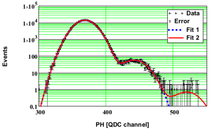
(a)

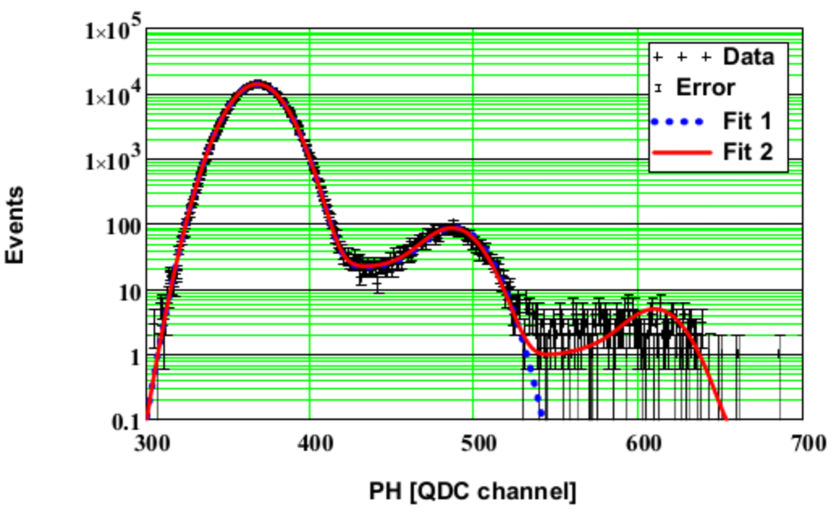
(b)

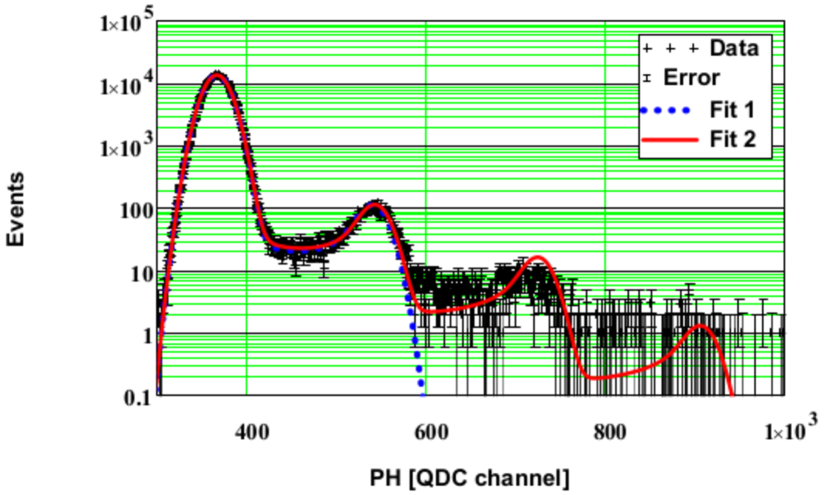
(c)

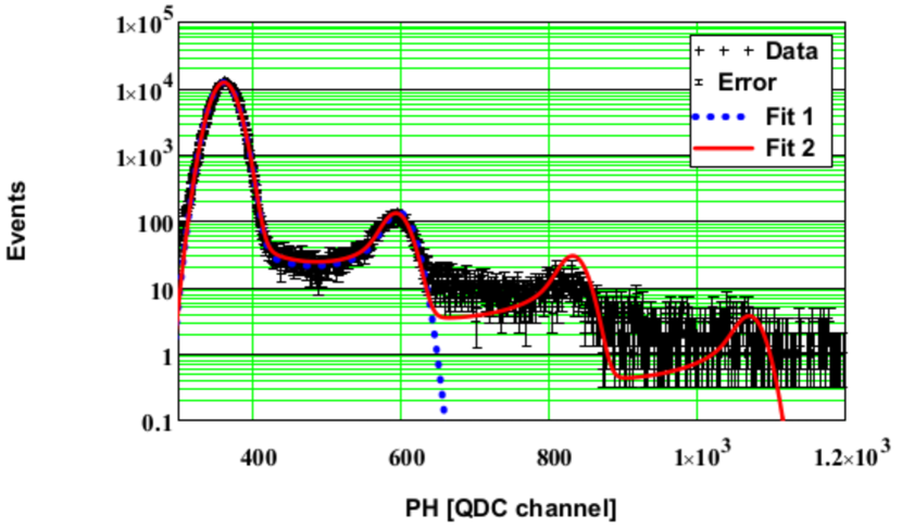
(d)

Figure 8: Pulse-height spectra measured without illumination with the results of the fits discussed in the text for (a) 29.5 V, (b) 31.0 V, (c) 33.0 V, and (d) 35.0 V. The dotted line is the model with single dark pulses only, the solid line the model, which includes multiple dark pulses and prompt cross-talk.

The standard way to analyse the $PH_{dark}$ spectra [4, 8] is to first determine $PH_{0}$, the position of the $npe=0$ peak using a fit by a Gauss function and take Gain from the analysis of the low-light spectra. Then, the fraction of events with $PH>(PH_{0}+0.5\,Gain)$, called $f_{0.5}$, and the fraction above $(PH_{0}+1.5\,Gain),\,f_{1.5}$, are determined. The dark-count rate is calculated using $DCR=f_{0.5}/t_{gate}$, and the correlated noise using $CN=f_{1.5}/f_{0.5}$. In order to obtain reliable results, the $npe=0$ and the $npe=1$ peaks have to be sufficiently separated, which, e.g. is not the case for the pulse-height spectrum at 29.5 V. However, this can be corrected by subtracting from $f_{0.5}$ the tail of the $npe=0$ Gauss function. Just subtracting the number of events in the $npe=0$ peak from the total number of events does not take into account the fraction of events with $PH$s between the pedestal and 1/2 the $npe=0$ peak and thus overestimates the dark-count rate. In this case the effective gate width, defined in Eq. 3, for the corresponding pulse-height threshold should be used.

For deriving the shape of the PH spectrum for a single dark-count pulse, we refer to Fig. 2b, which shows the mean PH integrated during the gate as a function of the time difference between the Geiger discharge and the start of the integration by the gate. Dark-count pulses are distributed randomly in time and their rate is DCR. The probability of pulses in the interval between PH and PH+dPH is proportional to the time interval $\mathrm{d}t=\mathrm{d}PH/|\mathrm{d}PH/\mathrm{d}t|$. For a normalised current pulse: $I_{norm}(t^{\prime})=1/\tau\cdot e^{-t^{\prime}/\tau}$ for $t^{\prime}\geq 0$ and $I(t^{\prime})=0$ for $t^{\prime}<0$, $PH_{norm}$ for a dark pulse at the time $t$ relative to the start of the integration by the gate is given by Eq. 1 with $Q_{0}=1$:

$$PH_{norm}(t)=\left\{\begin{array}[]{ll}e^{\frac{t}{\tau}}\,\big{(}1-e^{-\frac{t_{gate}}{\tau}}\big{)}&\hbox{\rm{for}\,\, $t<0$,}\\ \vspace{1mm}1-e^{-\frac{t_{gate}-t}{\tau}}&\hbox{\rm{for}\,\, $0\leq t<t_{gate},$}\\ 0&\hbox{\rm{for}\,\, $t\geq t_{gate}$.}\end{array}\right.$$ (11)

Next the time $t_{0}(<0)$ is introduced. $DCR$ pulses with $t\leq t_{0}$ are assigned to the pedestal, and $DCR$ pulses with $t_{0}<t\leq 0$ result in $PH_{norm}$ values in the range $PH_{norm}^{min}(t_{0})=e^{t_{0}/\tau}\,(1-e^{-t_{gate}/\tau})$ and $PH_{norm}^{max}=(1-e^{-t_{gate}/\tau})$. The $PH_{norm}$ distribution is given by $\mathrm{d}N/\mathrm{d}PH_{norm}=(\mathrm{d}N/\mathrm{d}t)/|\mathrm{d}PH_{norm}/\mathrm{d}t|=DCR/|\mathrm{d}PH_{norm}/\mathrm{d}t|$ with $PH_{norm}(t)$ given by Eq. 11 and the dark-count rate $\mathrm{d}N/\mathrm{d}t\equiv DCR$. The result is: d$N$/d$PH_{norm}=(DCR\cdot\tau)/PH_{norm}$. So far, correlated noise pulses, which shift entries from the $npe=1$ peak to higher values, are not taken into account. This will be discussed below. A similar derivation for DCR pulses occurring during the gate, $0\leq t\leq t_{gate}$, shows that the $PH_{norm}$ values are in the range 0 to $PH_{norm}^{max}$ with the distribution d$N$/d$PH_{norm}=(DCR\cdot\,\tau)/(1-PH_{norm})$.

Thus the $PH_{norm}$ distribution for random $DCR$ events with unit charge for $t_{0}\leq t\leq t_{gate}$ is

$$\frac{\mathrm{d}N}{\mathrm{d}PH_{norm}}=(DCR\cdot\,\tau)\cdot\Big{(}\frac{1}{PH_{norm}}+\frac{1}{1-PH_{norm}}\Big{)},$$ (12)

where the first term has to be evaluated for $PH_{norm}$ values between $PH_{norm}^{min}(t_{0})$ and $PH_{norm}^{max}$, and the second term between 0 and $PH_{norm}^{max}$. For DCR pulses outside of the time interval $t_{0}<t\leq t_{gate}$, $PH_{norm}$ is set to zero, and their contribution to the $PH_{norm}$ spectrum is:

$$\frac{\mathrm{d}\textit{N}}{\mathrm{d}PH_{norm}}=\big{(}1-DCR\cdot(t_{0}+t_{gate})\big{)}\cdot\delta(PH_{norm}=0),$$ (13)

where $\delta(x)$ is the Dirac delta function.

The choice of the value for $t_{0}$ is not critical, as long as $PH_{norm}^{min}(t_{0})$ is small compared to the width of the pedestal distribution. Increasing the value of $|t_{0}|$ only shifts events from Eq. 13 to Eq. 12 in the region of $PH_{norm}^{min}(t_{0})$. For the fits discussed below, $t_{0}=-a\cdot\tau$ with $a=5$ has been used, and it has been verified that varying $a$ between 3.5 and 7.5 does not affect the results.

Using a binned maximum-likelihood method, the measured $PH$ spectra in the region of the $npe=0$ and the $npe=1$ peaks are fitted by the sum of Eqs. 12 and 13 with $PH_{norm}$ scaled by $Gain=PH_{1}-PH_{0}$ and shifted by $PH_{0}$, convolved with a Gaussian of variance $\sigma^{2}$, and normalised to the number of measured events. As the function described by Eq. 12 is non continuous with sharp peaks at $PH_{norm}^{min}$ and $PH_{norm}^{max}$, which depend on the free parameter DCR, special care has to be taken for the convolution: Eq. 12 is evaluated in bins of constant width in $\ln(PH_{norm})$ for $PH_{norm}<0.5$, and in bins of constant width in $\ln(1-PH_{norm})$ for $PH_{norm}\geq 0.5$, and then convolved with Gaussians in the range $\pm\,5\,\sigma$. The free parameters of the fit are: the position of the $npe=0$ and $npe=1$ peaks, $PH_{0}$ and $PH_{1}$, the dark-count rate, $DCR$, the noise term, $\sigma$, and the normalisation.

The results of the fits for 29.5, 31.0, 33.0, and 35.0 V are shown as dotted lines, labeled "Fit 1", in Fig. 8. The data, in particular also the region in-between the $npe=0$ and the $npe=1$ peaks, which is populated by events with only partial overlap of the dark-count pulses with the gate, are well described. The number of entries between the $npe=0$ and the $npe=1$ peak is sensitive to the pulse decay time, $\tau$. The value $\tau=19.95$ ns, obtained from the delay curve in Sect. 3.1, provides a good description of the data. Changes by $\pm\,2.5$ ns spoil this agreement. Deviations between model and fit are observed at the low $PH$ tail of the $npe=0$ peak at 35 V. At this voltage the DCR is highest and the AC coupling produces deviations from the Gauss distribution of the pedestal peak. As the model considers neither multiple dark-count pulses nor correlated noise, the function drops to zero above the $npe=1$ peak. In addition, the value of DCR obtained from "Fit1" will be incorrect, if the probability for correlated noise is high.

Multiple dark-count pulses as well as prompt cross-talk and after-pulses from the dark-count pulses, result in PH values beyond the $npe=1$ peak. The following assumptions are made to derive a model, which considers PH values up to $npe=4$: Poisson statistics with a mean of $DCR\cdot(|t_{0}|+t_{gate})$ for the probability distribution of the dark-count pulses, and for each dark-count pulse a Borel branching process for the probability distribution of additional prompt cross-talk pulses. For further details we refer to Appendix B. For two reasons, after-pulses are not taken into account: As pointed out in Sect. 3.2, the time dependence of the after-pulses is not known, and the additional convolutions with delayed after-pulses significantly complicate the already complex model.

The results of binned maximum likelihood fits of the model to the data of 29.5, 31.0, 33.0, and 35.0 V are shown in Fig. 8 as solid lines, labeled "Fit 2". The model qualitatively describes the data also for npe > 1. However, in particular at higher voltages, there are significant discrepancies for PH values above the $npe=1$ peak: More events than predicted are observed in-between the $npe$ peaks, and the peaks in the data are less pronounced. We ascribe this to the neglect of the after-pulses.

Next the fit results are compared to the results of a method, which is similar to the standard method of determining the $DCR$. The $npe=0$ peak is fitted by a Gaussian in order to determine its mean value, $PH_{0}$, and its variance, $\sigma^{2}$. For $Gain$ the value determined from the $PH$ measurements with the SiPM illuminated by a pulsed LED, presented in Sect. 3.2, is used. The value of $f_{0.5}$ is obtained from the fraction of entries above $PH_{0}+0.5\cdot Gain$, and for $f_{0.5}^{corr}$ the fraction of entries in the tail of the Gauss function fitted to the $npe=0$ peak is subtracted from $f_{0.5}$. The dark-count rate is calculated using $DCR=f_{0.5}^{corr}/t_{gate}$, where $t_{gate}=100$ ns is used.

In Fig. 9a the DCR results for the two methods are shown as a function of voltage. The $DCR$ increases approximately linearly with voltage and reaches a value of about 220 kHz at 35 V, which is about 8 V above the breakdown voltage. At 29.5 V, where the $npe=0$ and $npe=1$ distributions overlap, the correction to $f_{0.5}$ is required. Above 29.5 V the $f_{0.5}$ and the $f_{0.5}^{corr}$ results are identical. The results of the DCR fit and the $f_{0.5}$ method agree up to a voltage of 32 V. For higher voltages the DCR fit results are somewhat lower, with a maximal difference of 7 % at 35 V. We assume that the reason for this discrepancy is the neglect of after-pulses in the DCR model, and consider the $f_{0.5}^{corr}$ results to be more reliable.

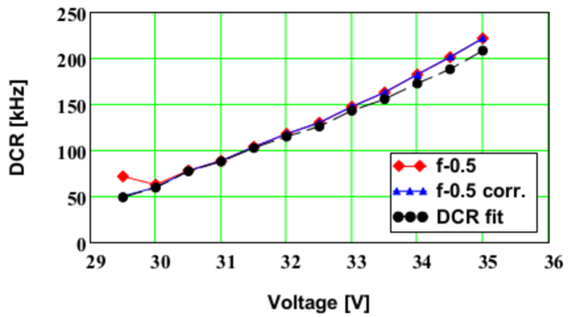
(a)

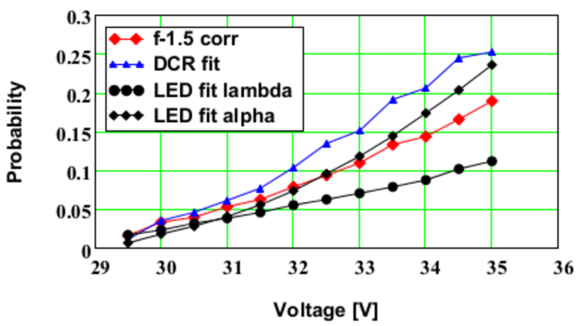
(b)

Figure 9: Comparison of the results of different methods of determining the voltage dependence of (a) the dark-count-rate, DCR, and (b) the cross-talk and after-pulse probabilities.

The correlated noise, CN, the combined effect of prompt cross-talk and after-pulsing, is determined using $CN=f_{1.5}/f_{0.5}^{corr}$, where $f_{1.5}$ is the fraction of entries in the DCR spectrum above $PH_{0}+1.5\,Gain$. The results, labeled "f-1.5 corr", are shown in Fig. 9b and compared to the results of the DCR fit, labeled "DCR fit". The DCR fit results are consistently higher, with a difference, which increases with voltage. Also shown are the results for the prompt cross-talk, labeled "LED fit lambda", and for the after-pulses, "LED fit alpha", from the fit to the LED data presented in Sect. 3.2. Shown are $1-e^{-\lambda}$ and $\alpha$, which correspond to the probability that a Geiger discharge causes one or more prompt discharges or an after-pulse, respectively. We find it difficult to interpret the differences, as they correspond to different quantities. However, as the DCR value from the fit is somewhat smaller than from the $f_{0.5}$ method, and the mean PH of the after-pulses is significantly smaller than for a single Geiger discharge, there may not be a real discrepancy.

The DCR fits also determine Gain. In Fig. 7b the results are compared to the values from the low-light fit. Typical differences are 1 to 2 %, with a maximal deviation of 2.9 %.

To summarise: A model has been developed, which attempts to describe the dark-count pulse-height spectra of SiPMs. It takes into account the random arrival times of dark pulses, multiple dark pulses and prompt cross-talk, but neglects after-pulses. The model is fitted to the data to determine the dark count rate, DCR, the gain, Gain, and the correlated noise, CN. A qualitative agreement with the measured spectra is achieved, however at higher voltages the region above the $npe=1$ peak is only approximately described. The differences are ascribed to the neglect of after-pulses. The comparison with the results of the standard method shows satisfactory agreement for DCR. For the correlated noise, differences of up to 25 % are found. We suspect that the cause is the neglect of the after-pulses, and consider the result of standard method more trustworthy. The values of Gain determined agree within < 3 % with the values determined from fits to the low-light spectra.

4 Application of the results

4.1 Resolution of photon detection and excess noise factor

The question addressed in this section is: At which voltage is the best resolution for the measurement of the number of photons from a light source achieved? This is e. g. relevant for the energy measurement using SiPMs coupled to scintillators. As a function of voltage, the photon-detection efficiency increases, but the excess noise from prompt cross-talk and after-pulsing also increases. Thus there will be an optimum. The relevant quantity for a given light source is the resolution, $Res=\sqrt{var}/mean$, where $mean$ is the mean and $var$ the variance of the PH distribution after subtracting the pedestal value. The dependence of Res on voltage for the low-light data is shown in Fig.10 a. In addition to $Res$ calculated from the moments of the measured PH spectra, labeled "Data", and from the fit curve, "Fit", the values for the Poisson distribution $Res_{Poisson}=1/\sqrt{\mu}$ and for the Generalised Poisson distribution $Res_{Gen.\,Poisson}=1/\sqrt{\mu\,(1-\lambda)}$, with the values determined in Sect. 3.2, are shown. Fig.10 a shows that between 34 and 35 V the improvement in resolution due to the relative increase of the photon-detection efficiency by 6.3 % is largely compensated by the increase in excess noise: $Res$ improves by 0.7 % only. It has been checked that the same voltage dependence of Res is obtained from the high-light data. Thus the optimal voltage is about 34 V. At higher voltages the resolution does not improve anymore, however, excess noise and dark-count rate increase significantly.

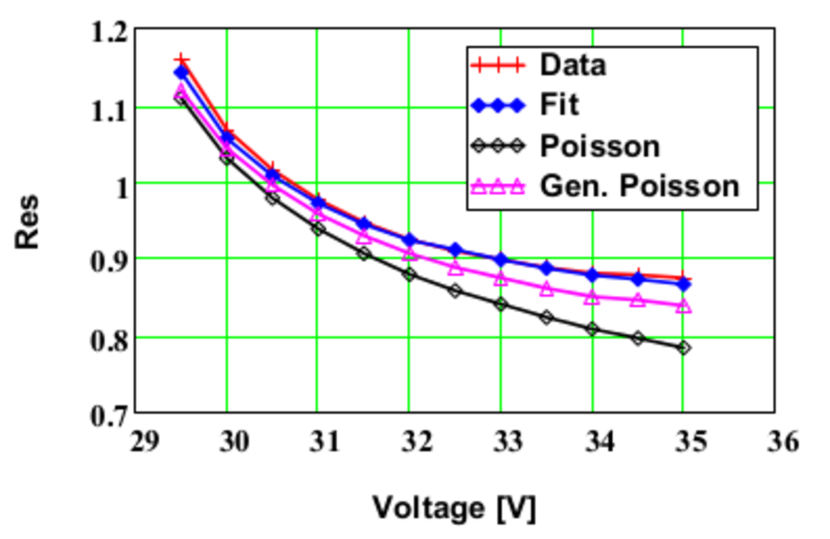
(a)

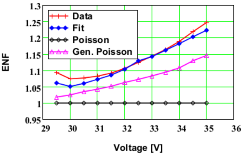
(b)

Figure 10: (a) Resolution, $Res=\sqrt{var}/mean$, for the pulse-height spectra of the low-light measurements, and (b) excess noise factor, ENF, for "Poisson", the Poisson distribution, "Gen. Poisson", the Generalised Poisson distribution with the parameters $\mu$ and $\lambda$ obtained in Sect. 3.2, "Fit", the fit function described in Sect. 3.2, and for "Data", calculated from the moments mean and var of the measured spectra.

To quantify the worsening of the resolution by excess noise, the excess-noise-factor, ENF, is commonly used. For a distribution $i$, $ENF_{i}$ is defined as

$$ENF_{i}=\big{(}var_{i}/mean_{i}^{2}\big{)}/\big{(}var_{Poisson}/mean_{Poisson}^{2}\big{)}=\mu\cdot(var_{i}/mean_{i}^{2}).$$ (14)

Fig.10b shows ENF_i of the low-light data for the Generalised Poisson distribution, "Gen. Poisson", for the fit function, "Fit", and for the measured spectra, "Data". The nonphysical increase of ENF for "Fit" and "Data" between 30 and 29.5 V is caused by the contribution of the pedestal width to var, which can be corrected by subtracting $\sigma_{0}^{2}$.

Eq. 14 also provides a simple way to determine $ENF$ using low-light spectra: Determine from the fraction of entries in the pedestal peak corrected for dark pulses, $f_{0}$, calculate $\mu=-\ln(f_{0})$ using Poisson statistics, evaluate $mean$ and $var$ from the spectrum, and use Eq. 14 to obtain ENF. The method has the advantage that it is simple to use and that no fits of pulse-height spectra are required. In Sect. 4.2 ENF is used to determine the average number of photons initiating a Geiger discharge and the SiPM gain from the moments mean and var of the pulse-height distribution measured with a pulsed light source. This method also works, when the individual npe peaks are not separated, and the standard methods of gain determination cannot be applied.

4.2 Determination of the number of detected photons and of the gain

For calibrating and monitoring a detector with many SiPMs, a simple and robust method to determine the mean number of detected photons, $\langle N_{\gamma}\rangle$, and the overall gain of the set-up is highly desirable. If the ENF values of the SiPMs are known, and the PH spectra from a pulsed light source are recorded in-situ, inverting Eq. 14 gives

$$\langle N_{\gamma}\rangle\equiv\mu=ENF\Big{(}\frac{mean^{2}}{var}\Big{)}.$$ (15)

The ENF values of the SiPMs can be determined before their installation into the detector with the method described in Sect. 4.1 using low-light PH-spectra. The proposed method also works, if the different npe peaks can not be separated, either because of a high number of photons, a coarse binning of the PH spectra, high dark-count rates e.g. due to radiation damage or operation at high temperature, or because of electronics noise. In the case of a significant noise, the variance of the pedestal distribution has to be subtracted from the variance of the spectrum recorded with light. We note that for a high number of photons, the Generalised Poisson distribution approaches a Gauss distribution, and a fit to the PH spectrum by a Gauss function can also be used for determining the mean and the variance.

In Fig. 11a the value of $\mu$ determined in Sect. 3.2, denoted "measured", is compared to the value calculated using Eq. 15, denoted "calculated", for the high-light data. Here $\sigma_{0}^{2}$ has been subtracted from $var$. The agreement is very good, demonstrating the validity of the method: The difference is 4 % at 29.5 V, and below 1 % above 30.5 V. The method described above is routinely used for the calibration of the MAGIC telescope [19].

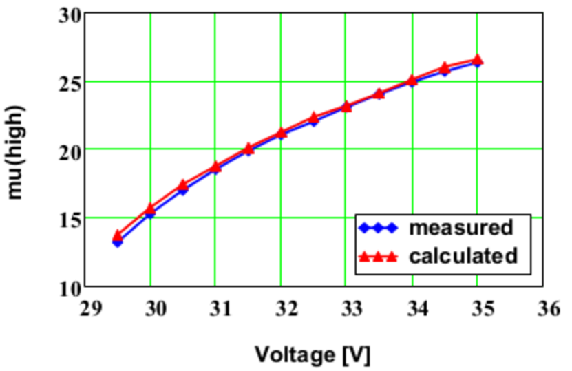
(a)

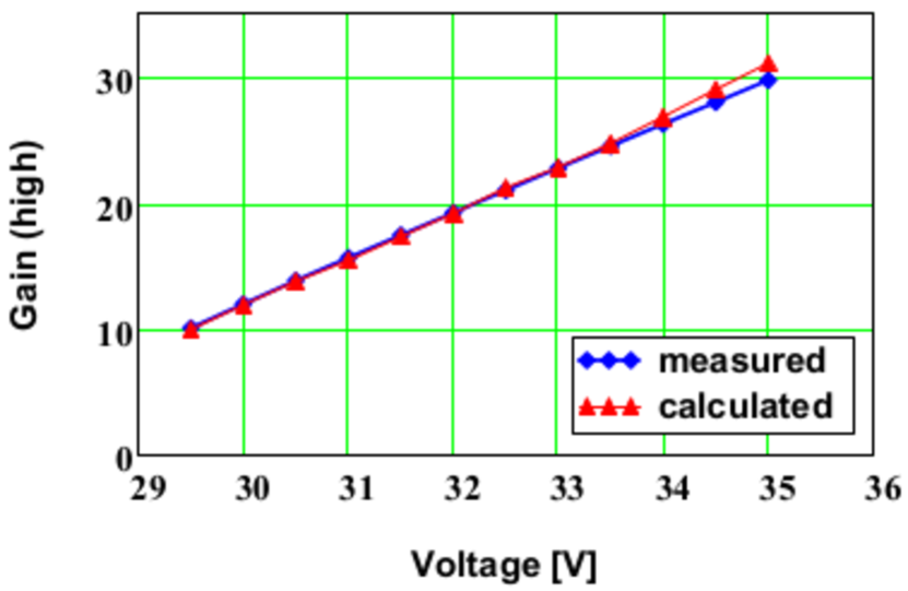
(b)

Figure 11: Comparison of (a) the mean number of detected photons, and (b) the gain for the high-light data using the fits (measured) and the method of the first and second moments of the measured pulse-height distributions, described in the text (calculated).

In a similar way, the combined gain of the SiPM and the readout, $Gain^{\prime}$, can be obtained, if the statistics of the combined effect of prompt cross-talk and after-pulsing is similar to the statistics of the Generalised Poisson distribution, GP. This is the case if the after-pulse probability $\alpha$ does not exceed $\approx 25$ %. The relation used is:

$$Gain^{\prime}=\frac{1}{ENF^{2}}\Big{(}\frac{var}{mean}\Big{)}.$$ (16)

It can be derived using the following properties of the Generalised Poisson distribution, GP: $mean_{GP}=\mu/(1-\lambda)$ and $var_{GP}=\mu/(1-\lambda)^{3}.$ Using Eq. 14 we find $ENF_{GP}=1/(1-\lambda)$. For the measured PH distribution with the gain, $Gain^{\prime}$, $var=Gain^{\prime\,2}\cdot\mu/(1-\lambda)^{3}=Gain^{\prime\,2}\cdot\mu\cdot ENF^{\,3}$, and $mean=Gain^{\prime}\cdot\mu/(1-\lambda)=Gain^{\prime}\cdot\mu\cdot ENF$, and the ratio results in Eq. 16.

In Fig. 11 b the gain values determined directly from the spectra, labeled "measured", are compared to the values "calculated" using Eq. 16. Up to a voltage of 33.5 V both values agree to within 1 %. For higher voltages, where the probability of after-pulses, $\alpha$, is higher than the probability of prompt cross-talk, $\lambda$, as shown in Fig. 7 d, the gain values are overestimated. The maximum deviation is 4.5 % at 35 V. As can be seen from Fig. 5d, for the high-light data at 35 V, the individual npe peaks are not separated, and neither $\langle N_{\gamma}\rangle$ nor $Gain^{\prime}$ could have been determined using the standard methods.

To summarise: Using the method to determine the excess-noise-factor, ENF, described in Sect. 4.1, the combined gain of the SiPM and the readout, and the mean number of detected photons, $\langle N_{\gamma}\rangle$, can be obtained from the mean and the variance of the measured pulse-height spectra. The method is simple and also applicable for high $\langle N_{\gamma}\rangle$ values, as long as saturation effects due to the finite number of pixels can be ignored. Taking saturation effect into account, appears not to be too complicated.

5 Conclusions and outlook

For a KETEK SiPM with 4384 pixels of $15\,\upmu$m$\times 15\,\upmu$m pitch, the pulse-height spectra have been measured for voltages between 2.5 and 8 V above the break-down voltage at 20^∘C for two different intensities of pulsed light and without illumination. A model for analysing the pulse-height spectra measured with pulsed light has been developed, which includes the statistics of the photons triggering Geiger discharges, the statistics of prompt cross-talk, and the pulse-height distribution and statistics of after-pulses. The model describes the measured pulse-height spectra, including the "background". As far as we know, such a description has not yet been achieved so far. From the agreement of the model with the data it is concluded: The statistics of the cross-talk from a primary Geiger discharge can be described by a Borel distribution, which results in a Generalised Poisson distribution for the combined statistics of primary Geiger discharges and cross-talk. The statistics of after-pulses from a Geiger discharge can be described by a binomial distribution. The pulse-height distribution of the after-pulses has been derived from the data.

By fitting the model to the pulse-height spectra, the voltage dependence of the SiPM gain, the number of photons initiating Geiger discharges, the cross-talk and the after-pulse probability were obtained. The results were used to determine the excess-noise factor due to prompt cross-talk and after-pulses, and the voltage for optimal light-yield resolution.

Based on the detailed understanding of the SiPM statistics, a method for calibrating and monitoring the number of photons initiating Geiger discharges and the combined gain of the system SiPM and readout is demonstrated, which appears suitable for detectors with a large number of SiPMs, like calorimeters. It uses the mean and the variance of the pulse-height spectra measured in-situ from a pulsed light source, and the excess noise factor, which can be determined in a straight-forward way as part of the pre-installation quality control of the SiPMs. For the SiPMs investigated, the accuracy of the gain and the number of photons determined agrees to better than 5 % with the fit results, when the light intensity is changed by a factor of 16.

A model for the pulse-height spectra of dark counts is developed, which takes into account the random occurrence of dark pulses and prompt cross-talk, but neglects after-pulses. It provides a good description of the peaks corresponding to zero and one Geiger discharges, and the region in-between, and allows to determine the gain, the dark-count rate and the cross-talk probability. The spectra above the one Geiger-discharge peak are only qualitatively described, indicating that also the effect of after-pulses has to be implemented in the model. It is shown that the SiPM gain can be determined from pulse-height spectra measured in the dark, without the need of a pulsed light source, which could be of interest for detectors with a large number of SiPMs.

6 List of References

Appendix A Appendix A: Pulse-height distribution for an exponential after-pulse probability

In Sect. 3.2 we have stated that that the observed exponential PH distribution for AP pulses for the KETEK SiPM was not expected. In this Appendix we derive the dependence expected for an exponential time dependence of the after-pulse probability. To simplify the formulae we assume $Gain=1$, define $PH_{AP}$ as the additional PH from the after-pulse, measure the time $t$ from the start of the Geiger discharge, which causes the after-pulse and assume that $t=0$ is also the start of the integration by the QDC. For the time dependence of the AP probability density an exponential is assumed:

$$\frac{\mathrm{d}p_{AP}}{\mathrm{d}t}=\frac{1}{\tau_{AP}}e^{-t/\tau_{AP}}.$$ (17)

For $PH_{AP}(t)$, the $PH$ of an after-pulse at time $t$ after the primary pulse

$$PH_{AP}(t)\left\{\begin{array}[]{ll}\vspace{2mm}=\big{(}1-e^{-t/\tau}\big{)}\cdot\int\limits_{0}^{t_{gate}-t}\big{(}\frac{e^{-t^{\prime}/\tau}}{\tau}\big{)}\,\mathrm{d}t^{\prime}=\\ =1+e^{-t_{gate}/\tau}-2\,e^{-t_{gate}/(2\,\tau)}\,\cosh\big{(}\frac{t_{gate}/2-t}{\tau}\big{)}\end{array}\right.$$ (18)

is assumed. The first term of the upper line of Eq. 18 describes the reduction of $PH_{AP}$ due to the recharging of the pixel with the time constant $\tau$ after a Geiger discharge, and the second term the fraction of the AP signal integrated during the QDC gate of duration $t_{gate}$. The function $PH_{AP}(t)$ is symmetric around $t=t_{gate}/2$, zero at $t=0$ and $t=t_{gate}$, and the value of the maximum at $t=t_{gate}/2$ is:

$$PH_{AP}^{max}=\big{(}1-e^{-t_{gate}/(2\,\tau)}\big{)}^{2}.$$ (19)

To derive the probability density distribution $\mathrm{d}p_{AP}/\mathrm{d}PH_{AP}$, we use $\frac{\mathrm{d}p_{AP}}{\mathrm{d}PH_{AP}}=\frac{\mathrm{d}p_{AP}}{\mathrm{d}t}/|\frac{\mathrm{d}PH_{AP}}{\mathrm{d}t}|$ to obtain

$$\frac{\mathrm{d}p_{AP}}{\mathrm{d}PH_{AP}}=\frac{\tau}{\tau_{AP}}\,\frac{e^{-t(PH_{AP})/\tau_{AP}}}{2\,e^{-t_{gate}/(2\,\tau)}|\sinh\big{(}\frac{t_{gate}/2-t(PH_{AP})}{\tau}\big{)}|},$$ (20)

which is valid in the $PH_{AP}$ range between 0 and $PH_{AP}^{max}$. The function $t(PH_{AP})$ is obtained by inverting Eq. 18. For more than one AP, the probability distribution has to be convolved with itself, and finally the complete probability density is convolved by a Gaussian to account for noise. The convolutions are performed using the Fast-Fourier-Transform. We note that in this model, for certain values of the ratio $t_{gate}/\tau$, peaks, caused by after-pulses, appear at $PH_{AP}^{max}$ in-between the $npe$ peaks. Such intermediate peaks have actually been observed for a MPPC from Hamamatsu.

Appendix B Appendix B: Fit function for the DCR spectra

In this appendix we sketch the derivation of the formulae used in Sect. 3.3 to fit the $PH_{dark}$ spectra including the $npe=4$ peak. To simplify the formulae, we use the normalised pulse height, $x$, with $x=0$ the mean of the pedestal and $x=1$ the mean of the $npe=1$ peak, and derive the formulae without smearing due to electronic noise and gain differences between pixels.

We call $f^{(1)}(x)$ the normalised $PH$ probability distribution derived from Eq. 12. For i $DCR$ pulses in the time interval between $t_{0}$ and $t_{gate}$ and no prompt cross-talk, the normalised $PH$ distribution, $f^{(i)}(x)$, is the $i$-fold convolution of $f^{(1)}(x)$, calculated using the $i$-th power of the Fourier transform of $f^{(1)}(x)$. Prompt cross-talk just stretches the $x$ values of the $PH$ probability distribution, and the distribution for the $j$-fold cross-talk of a single $DCR$ pulse is given by $h^{(j)}(x)=f^{(1)}((j+1)\cdot x)/(j+1)$. The distributions for arbitrary combinations of $DCR$ and cross-talk pulses are convolutions of $f^{(i)}(x)\otimes h^{(j)}(x)$. Examples are shown in Table 1, which presents for the $i,j$ values possible for $npe\leq 4$ the combinatoric factors and the corresponding functions. The sum of these functions multiplied with the appropriate combinatoric factors, $Comb$, and the probability products $Poisson\cdot Borel$ gives the normalised $PH$ spectrum. Finally, after the transformation $x\rightarrow PH_{0}+Gain\cdot x$ and the convolution with a Gauss function, the resulting function is fitted to the measured $PH$ distributions.

Table 1: Parameters and functions used for the fit function for the $PH_{dark}$ spectrum; $npe$: total number of Geiger discharges including prompt cross-talk in the time interval $t_{0}$ to $t_{gate}$; $P_{i}$: Poisson probability for $i$ primary dark pulses, $B_{j}$: Borel probability for $j$ prompt cross-talk pulses, $Comb$: number of permutations for the given configuration, and Function: $PH$ distribution for the given configuration.

$npe$	$Comb$	$Poisson_{i}$	$Borel_{j}$	Function
0	1	0	$-$	$\delta(x)$
1	1	$P_{0}$	$B_{0}$	$f^{(1)}$
2	1	$P_{1}$	$B_{1}$	$h^{(1)}$
2	1	$P_{2}$	$(B_{0})^{2}$	$f^{(2)}$
3	1	$P_{1}$	$B_{2}$	$h^{(2)}$
3	2	$P_{2}$	$B_{0}\cdot B_{1}$	$f^{(1)}\otimes h^{(1)}$
3	1	$P_{3}$	$(B_{0})^{3}$	$f^{(3)}$
4	1	$P_{1}$	$B_{3}$	$h^{(3)}$
4	2	$P_{2}$	$B_{0}\cdot B_{2}$	$f^{(1)}\otimes h^{(2)}$
4	1	$P_{2}$	$(B_{1})^{2}$	$h^{(1)}\otimes h^{(1)}$
4	3	$P_{3}$	$(B_{0})^{2}\cdot B_{1}$	$f^{(2)}\otimes h^{(1)}$
4	1	$P_{4}$	$(B_{0})^{4}$	$f^{(4)}$

References

- [1] P. Buzhan et al., Silicon photomultiplier and its possible applications, Nuclear Instruments and Methods in Physics Research Section A 504 (2003) 48–52, doi:10.1016/S0168-9002(03)00749-6.
- [2] J. Haba, Status and perspectives of Pixelated Photon Detector (PPD), Nuclear Instruments and Methods in Physics Research Section A 595 (2008) 154–260, doi:10.1016/j.nima.2008.07.061.
- [3] D. Renker and E. Lorenz, Advances in solid state photon detectors, 2008 JINST 4 P04004, doi10.1088/1748-0221/4/04/P04004.
- [4] P. Eckert et al., Characterisation studies of silicon photomultipliers, Nuclear Instruments and Methods in Physics Research Section A 620 (2010) 217–226, doi:10.1016/j.nima.2010.03.169.
- [5] C. Piemonte et al., Development of an automatic procedure for the characterization of silicon photomultipliers, 2012 IEEE Nuclear Science Symposium and Medical Imaging Conference Record (NSS/MIC) N1-206 428–432, 10.1109/NSSMIC.2012.6551141
- [6] A. Biland et al., Calibration and performance of the photon sensor response of FACT – the first G-APD Cherenkhov telescope, 2014 JINST 9 P10012, doi10.1088/1748-0221/9/10/P10012.
- [7] V. Arosio, al., An Educational Kit Based on a Modular Silicon Photomultiplier System, arXiv:1308.3622.
- [8] Ch. Xu et al., Influence of X-ray irradiation on the properties of the Hamamatsu silicon photomultiplier S10362-11-050C, Nuclear Instruments and Methods in Physics Research Section A 762 (2014) 149–161, doi:10.1016/j.nima.2014.05.112.
- [9] Ch. Xu, Study of the Silicon Photomultipliers and Their Applications in Positron Emission Tomography, PhD thesis, University of Hamburg, April 2014.
- [10] KETEK, Hofer Str. 3, D-81737 Munich, Germany http://www.ketek.net.
- [11] V. Chmill, E. Garutti, R. Klanner and J. Schwandt, Study of the breakdown voltage of SiPMs, Nuclear Instruments and Methods in Physics Research Section A 845 (2017) 56–59, doi:10.1016/j.nima.2016.04.047.
- [12] M. S. Nitschke, Characterization of Silicon Photomultipliers before and after Neutron Irradiation, MSc Thesis, University of Hamburg, June 2016.
- [13] Fast Pulse Preamplifier, Model 6954. Phillips Scientific, 31 Industrial Ave., Mahwah, NJ 07430.
- [14] CAEN qS srl, Via Vetraia 11, 55049 - Viareggio (LU) - Italy, http://www.caen.it.
- [15] Pulse Pattern Generator 8110A, 150 MHz, Keysight Technologies, www.keysight.com.
- [16] Digital Delay Generator DG645, Stanford Research Systems, Inc., 1290-C Reamwood Avenue, Sunnyvale, California 94089.
- [17] P. C. Consul and G. C. Jain, A generalization of the Poisson Distribution, Technometrics 15(4) (1973) 791–799.
- [18] S. Vinogradov, Analytical models of probability distribution and excess noise factor of solid state photomultiplier signals with crosstalk, Nuclear Instruments and Methods in Physics Research Section A 695 (2012) 247–251, doi:10.1016/j.nima.2011.11.086.
- [19] M. Gaug, H. Bartko, J. Cortina and J. Rico, Calibration of the MAGIC Telescope, 29th International Cosmic Ray Conference Pune (2005) 101–106.