Numerical Solution of a Coefficient Inverse Problem with Multi-Frequency Experimental Raw Data by a Globally Convergent Algorithm

Abstract

We analyze in this paper the performance of a newly developed globally convergent numerical method for a coefficient inverse problem for the case of multi-frequency experimental backscatter data associated to a single incident wave. These data were collected using a microwave scattering facility at the University of North Carolina at Charlotte. The challenges for the inverse problem under the consideration are not only from its high nonlinearity and severe ill-posedness but also from the facts that the amount of the measured data is minimal and that these raw data are contaminated by a significant amount of noise, due to a non-ideal experimental setup. This setup is motivated by our target application in detecting and identifying explosives. We show in this paper how the raw data can be preprocessed and successfully inverted using our inversion method. More precisely, we are able to reconstruct the dielectric constants and the locations of the scattering objects with a good accuracy, without using any advanced a priori knowledge of their physical and geometrical properties.

Keywords. experimental multi-frequency data, backscatter data, raw data, coefficient inverse problem, globally convergent numerical methods

AMS subject classification. 35R30, 78A46, 65C20

1 Introduction

We are interested in a Coefficient Inverse Problem (CIP) with real world applications, including the detection and identification of explosives, nondestructive testing and material characterization. A new globally convergent numerical method for solving such a CIP has been recently developed by our group in [19]. Numerical study in [19] was conducted for computationally simulated data. In this paper, we study the performance of this method for the case of experimental raw data. These data were collected using a microwave scattering facility at the University of North Carolina at Charlotte.

More precisely, we consider the CIP of reconstruction of physical and geometrical properties of three-dimensional objects from experimental multi-frequency data without using any detailed a priori knowledge of those objects. Our study is mainly motivated by potential applications in detection and identification of explosives such as, e.g., anti-personnel mines and improvised explosive devices (IEDs), see [28, 33]. These targets are placed in air, and the measured data are the backscatter corresponding to a single incident wave at multi-frequencies. In addition, we note that IEDs are also often buried under the ground for which one needs to study the corresponding inverse problem of determining buried objects. This topic is subject to a future publication.

The idea here is to determine the dielectric constants of targets. The knowledge of dielectric constants might serve in the future classification algorithms as a piece of information, which would be an additional one to those commonly currently used in the radar community. Indeed, this community relies now only on the intensity of radar images, see, e.g., [20, 29]. It is well known that the question of a reliable differentiation between explosives and clutter is not yet addressed satisfactory in the radar community. So, estimates of dielectric constants and shapes of targets combined with the image intensity and other parameters might lead in the future to such classification algorithms, which would address this question better. The second potential application of our study is in nondestructive testing and materials characterization.

A Coefficient Inverse Problem is the problem of recovering a coefficient of a partial differential equation from boundary measurements of its solutions. There is a large body of the literature on imaging methods for reconstructing geometric information about targets, such as their shapes, sizes and locations. We refer to, e.g., [3, 2, 8, 9, 11, 18, 23, 24, 22, 27] and references therein for well-known imaging techniques in inverse scattering such as level set methods, sampling methods, expansion methods, and shape optimization methods. However, for detecting or identifying, for instance, IEDs, the physical properties of the targets (in our model, the dielectric constants), would play a more important role [33]. Furthermore, determining the spatially distributed dielectric constants, which is of our main interest, is known to be a more difficult task since CIPs are, in general, highly nonlinear and severely ill-posed.

Among the inversion methods developed for solving the CIPs, the two probably most well known approaches are nonlinear approximation schemes and weak scattering approximation methods such as Born approximation and physical optics. The weak scattering approximation is not applicable to the inverse problem under consideration, where the scattering objects can be strong scatterers. Regarding the nonlinear optimization approaches or also known as iterative solution methods, we refer to, e.g., [13, 10, 14] and references therein. It is well-known that the convergence for this class of methods typically requires a good a priori initial approximation of the exact solution, that is, the starting point of iterations should be chosen to be sufficiently close to the solution. Hence, we call such methods locally convergent. We note that in our desired applications such a priori knowledge is not always available.

This limitation of nonlinear optimization approaches is avoided in the so-called approximately globally convergent method (globally convergent method, for short, or GCM), which has been recently introduced, see [4]. The GCM, which does not use optimization schemes, aims to provide a good approximation to the solution of the coefficient inverse problem without using any advanced a priori knowledge of the solution. More precisely, the concept “approximate globally convergence” can be understood in the language of functional analysis as follows: under a reasonable approximate mathematical assumption the method provides at least one point in a sufficiently small neighborhood of the exact coefficient without a priori knowledge of any point in this neighborhood. The accuracy of the approximation or the distance between those points and the exact solution depends on the error in the data and some parameters of the discretization. We point out that the fact of the proximity of that point to the correct coefficient, which was achieved without any a priori knowledge of that small neighborhood, is the main advantage of our globally convergent method over locally convergent ones. Indeed, as soon as one knows a point in a sufficiently small neighborhood of the true solution, one can refine it via a locally convergent method, see, e.g., [4, Chapter 4]. The latter, however, is outside of the scope of the current publication. We refer to [4, Theorem 2.9.4] for more details about the definition of the global convergence as well as a rigorous mathematical analysis of the global convergence of the method relying on an approximate mathematical framework.

In previous works of the GCM summarized in [4], the model of hyperbolic wave type equations is considered and the time-domain problem is converted into the pseudo-frequency domain problem via the Laplace transform. Since the Laplace transform used in the method has an exponentially decaying kernel, one likely loses some information in taking this transform of the (far field) measured data. Therefore, we exploit the Fourier transform to improve the performance of the GCM and to extend its direct application to multi-frequency data, which is common in applications to materials characterization. This leads us to study a new GCM in [19]. More precisely, in the latter paper, we developed a GCM for solving the CIP for the Helmholtz equation with multi-frequency data. The main difficulty in developing this new GCM is to work with complex-valued functions where the maximum principle, which plays an important role in the previous GCM [4], is no longer applicable.

As a continuation of the work of [19], the goal of this paper is to analyze the performance of our new GCM for multi-frequency experimental raw data. There are some major new features of the present paper:

1. The globally convergent approach together with its advantages makes this work different from previously known locally convergent methods.

2. This paper is the first one where we study the experimental multi-frequency data for the new GCM of [19].

3. For the multi-frequency raw data in this paper, we developed a new data preprocessing procedure, which is discussed later in this section. This procedure is substantially different from that of the time domain data in [30].

4. Recall that this is the CIP with a minimal amount of multi-frequency raw data (backscatter data associated to a single incident wave) and we are not aware of any literature that addresses the numerical solution of this problem without using any advanced a priori knowledge of the solution.

We also refer to [20, 4, 30] for our works on time-domain measured data for the previous GCM. Furthermore, we remark that our measured data are stable only on a small interval of frequencies surrounding the central frequency of 3.1 GHz, see section 4.2.2. Therefore, transforming these data into time domain by the inverse Fourier transform may lead to a large inaccuracy in the time-dependent data obtained. That means that time domain inversion techniques including the previous GCM [4] are not a good candidate for the inverse problem under consideration.

Keeping in mind our desired application to the detection and identification of mines and IEDs, we did not arrange any “special” conditions for our experiments, which would eliminate parasitic signals scattered by some objects, which are outside of our interest. Thus, our data have been collected in a regular room with the presence of office furniture, computers, wifi signals, air conditioning, etc., see Figure 1. Therefore, the measured data are contaminated by a significant amount of noise. The latter is a major challenge for any inversion method. We refer to section 4.2 for more details about the sources of the noise. We note that conventional data denoising techniques are not helpful here due to the rich structure of the measured data. We hence present in this paper a new heuristic data preprocessing procedure. This procedure aims to make the raw data look somewhat similar to the corresponding computationally simulated data. The latter is done basically via a sort of “distilling” signals reflected by the targets of our interest from the rest of the measured signals. The preprocessed data are then used as the input for the GCM. Our test results show that the GCM can reconstruct with a good accuracy the dielectric constants of the scattering objects as well as their geometric information such as location. In doing so, we do not use any detailed a priori knowledge on physical and geometrical properties of the targets.

We also mention reconstruction algorithms of [1, 25, 17, 16] for coefficient inverse problems, which obtain unknown coefficients without using any advanced a priori knowledge of their neighborhood. These algorithms use data resulting from multiple measurement events, i.e., the Dirichlet-to-Neumann map data. On the other hand, our GCM uses the data corresponding to a single incident plane wave.

The paper is organized as follows. In section 2, we state the forward and inverse problems. Section 3 is devoted to a short description of the globally convergent method. We describe in section 4 the data collection and the steps of data preprocessing. Section 5 contains a description of the numerical implementation of the method and a summary of reconstruction results. Summary of results can be found in section 6.

2 The forward and inverse problems

In this section we formulate the forward and inverse problems for scattering of electromagnetic waves by a penetrable inhomogeneous medium in $\mathbb{R}^{3}$ in a certain range of the frequency $\omega$. Below ${\bf x}=\left(x,y,z\right)\in\mathbb{R}^{3}.$ We assume that the scattering medium, which occupies a bounded domain $D\subset\mathbb{R}^{3}$, is isotropic, non-magnetic and that it is characterized by the spatially distributed dielectric constant $\varepsilon_{r}({\bf x})$, which is also called the relative permittivity. Our forward problem consists in finding the function $u\left({\bf x},k\right)$ from the following conditions:

$$\Delta u+k^{2}\varepsilon_{r}({\bf x})u=0,\quad{\bf x}\in\mathbb{R}^{3},$$ (1)

$$u=e^{ikz}+u_{\mathrm{sc}},$$ (2)

$$\lim_{r\rightarrow\infty}r\left(\frac{\partial u_{\mathrm{sc}}}{\partial r}-iku_{\mathrm{sc}}\right)=0,\quad r=|{\bf x}|.$$ (3)

Here $k=\omega/c$ is the wavenumber with the speed of light $c$. Here $u\left({\bf x},k\right)$ is one of components of the electric field. The total wave field $u$ is the sum of the scattered field $u_{\mathrm{sc}}$ and the incident field $u_{\mathrm{inc}}=e^{ikz}$, propagating along the $z$-direction towards the scattering medium. We note that the scattered field $u_{\mathrm{sc}}$ satisfies the Sommerfeld radiation condition (3), which guarantees that it is an outgoing wave.

Remark 1

To justify the description of the propagation of electromagnetic waves by a the single Helmholtz equation (1) rather than by the full Maxwell’s equation, we refer for instance to [6, Chapter 13]. It is shown there that if the function $\varepsilon_{r}({\bf x})$ varies slowly enough on the scales of the wavelength, then the scattering problem for the Maxwell’s equations can be approximated by the scattering problem for the Helmholtz equation for a certain component of the electric field. An additional justification comes out of the accuracy of our reconstruction results for our experimental data, see Table 2 in section 4.

We assume that the function $\varepsilon_{r}({\bf x})$ is frequency-independent, real-valued, $\varepsilon_{r}\in C^{1}(\mathbb{R}^{3})$ and that there exists a positive constant $\overline{\varepsilon}>1$ such that

$$1\leq\varepsilon_{r}({\bf x})\leq\overline{\varepsilon},\qquad\varepsilon_{r}({\bf x})=1\quad\text{for all }{\bf x}\in\mathbb{R}^{3}\setminus\overline{D}.$$ (4)

The latter condition in (4) means that the medium outside of $D$ is homogeneous. It is well-known that the forward problem (1)–(3) of finding the total field $u$, given $u_{\mathrm{inc}}$ and $\varepsilon_{r}$, is uniquely solvable for $u\in C^{2}(\mathbb{R}^{3})$, see [12, Chapter 8]. Our assumption of the frequency independence of $\varepsilon_{r}$ is justified by the fact that in our inverse algorithm of [19] we actually work on a small interval of wavenumbers $k$. Our direct experimental measurements of the dielectric constants of targets have shown that they vary slowly with respect to $k$ on small $k-$intervals.

We now formulate our inverse problem which is the main subject of the paper. To this end let us define $\Omega\subset\mathbb{R}^{3}$ as a convex bounded domain with its regular boundary $\partial\Omega$ such that $D\subset\Omega,\partial D\cap\partial\Omega=\varnothing$. Let $\underline{k}$ and $\overline{k}$ be positive constants such that $\underline{k}<\overline{k}$. Let $\Gamma\subset\partial\Omega$ be the part of the boundary $\partial\Omega$ which corresponds to the backscatter side of $\Omega$. We consider the following inverse problem or also the coefficient inverse problem:

Coefficient Inverse Problem. Assume that we are given a multi-frequency backscatter data $g({\bf x},k)$ defined by

$$g({\bf x},k):=u({\bf x},k),\quad\text{for }{\bf x}\in\Gamma,k\in[\underline{k},\overline{k}],$$ (5)

where $u({\bf x},k)$ is the total field in the forward problem (1)–(3). Determine the relative permittivity $\varepsilon_{r}({\bf x})$ for ${\bf x}\in\Omega$.

Remark 2

The mathematical justification of the globally convergent method [19] has been done only for measurements on the entire boundary $\partial\Omega$. Thus, in our theoretical derivation we assume that the function $g({\bf x},k)$ is given on $\partial\Omega$. In our numerical implementation we would need to complement the backscatter data on the rest of the boundary $\partial\Omega$. We show how this is done in section 5.2.

Since we consider only a single direction of the incident plane wave $u_{\mathrm{inc}}({\bf x},k)$, then this is an inverse problem with single measurement data. Given such data, we emphasize that in our coefficient inverse problem we aim to reconstruct the coefficient $\varepsilon_{r}({\bf x})$ using a numerical algorithm. The question whether $\varepsilon_{r}({\bf x})$ can be uniquely determined from the data is outside of the scope of this paper. This is also one of the fundamental theoretical questions in the field of inverse problems.

The first uniqueness result for multidimensional coefficient inverse problems with single measurement data was established in [7], where the authors introduced a method based on Carleman estimates. This method has been extensively studied by a number of authors for uniqueness theorems in inverse problems with a finite number of measurements. We refer to [34, 4] and references therein for surveys of this method and uniqueness results. However, the technique of [7] works only if a non-vanishing function $f({\bf x})$ stands in the right hand side of (1). Hence, we always assume below that uniqueness result holds true.

We end up this section with the Lippmann-Schwinger equation formulation for the forward problem (1)–(3). Let the wavenumber $k$ be fixed in (1)–(3). The Green’s function in free space for the forward problem is given by

$$\Phi_{k}({\bf x},{\bf y})=\frac{\exp{(ik|{\bf x}-{\bf y}|)}}{4\pi|{\bf x}-{\bf y}|},\quad{\bf x}\neq{\bf y}.$$

It is well-known that, see [12, Chapter 8], the forward problem (1)–(3) is equivalent to the Lippmann-Schwinger equation

$$u({\bf x})=e^{ikz}+k^{2}\int_{\Omega}\Phi_{k}({\bf x},{\bf y})(\varepsilon_{r}({\bf y})-1)u({\bf y})\mathrm{d}{{\bf y}},\quad{\bf x}\in\mathbb{R}^{3}.$$ (6)

We observe from (6) that if we know the function $u({\bf x})$ in $\Omega$, then we can just extend it to ${\bf x}\in\mathbb{R}^{3}\setminus\overline{\Omega}$ by the integration in (6). Hence, to solve (6), it is sufficient to find the function $u({\bf x})$ only for points ${\bf x}\in\Omega$. This integral equation plays an important role for the convergence analysis of [19] as well as for the numerical algorithm of the globally convergent method, see section 3.3.

3 The globally convergent numerical method

We describe in this section the globally convergent method together with its numerical algorithm. We essentially rely on the paper [19] where a theoretical study for this version of the method has been carried out for measurement data on the entire boundary $\partial\Omega$. Therefore, even though we are given only experimental backscatter data, we will assume that we have the complete data on $\partial\Omega$ for our description of the method.

3.1 Integro-differential equation formulation

The first crucial step for the construction of the GCM is to formulate the coefficient inverse problem as a nonlinear integro-differential equation. This is different from locally convergent methods with iterative optimization processes which typically rely on least-squares formulation. We describe in this section how to derive this integro-differential equation using the structure of the forward problem and a change of variables. To follow the theory of [19], we assume below that numbers $\underline{k},\overline{k}$, which are given in (5), are sufficiently large and $k\in[\underline{k},\overline{k}]$. It was shown in [19] that $u({\bf x},k)\neq 0$ for ${\bf x}\in\Omega$ as long as $k$ is sufficiently large.

It has been shown in [19] that there exists a function $v({\bf x},k)\in C^{2}(\overline{\Omega})$ such that $u({\bf x},k)=e^{v({\bf x},k)}$. Substitution of $u({\bf x},k)=e^{v({\bf x},k)}$ in the Helmholtz equation (1) and a simple calculation give

$$\Delta v+\nabla v\cdot\nabla v=-k^{2}\varepsilon_{r}({\bf x}).$$ (7)

From now on, for the sake of presentation, we write $a\cdot a$ as $a^{2}$ for a complex-valued vector $a\in\mathbb{C}^{3}$. We eliminate $\varepsilon_{r}({\bf x})$ from (7) by the differentiation of both sides of this equation with respect $k$, which is similar to the first step of the method of [7]. We obtain

$$\Delta\partial_{k}v+2\nabla\partial_{k}v\cdot\nabla v=\frac{2\Delta v+2(\nabla v)^{2}}{k}.$$ (8)

It is seen that if we can somehow find $v$ from the latter equation, then $\varepsilon_{r}$ can be computed via (7). We observe in (8) that $\partial_{k}v$ and $v$ are related as

$$v({\bf x},k)=-\int_{k}^{\overline{k}}\partial_{k}v({\bf x},s)\mathrm{d}s+v({\bf x},\overline{k}).$$

Defining

$$q({\bf x},k):=\partial_{k}v({\bf x},k),\quad V({\bf x}):=v(\mathbf{x},\overline{k}),$$ (9)

and substituting in (8), we obtain a nonlinear integro-differential equation for $q$

$$\frac{k}{2}\Delta q({\bf x},k)+k\nabla q({\bf x},k)\cdot\left(-\int_{k}^{\overline{k}}\nabla q({\bf x},s)\mathrm{d}s+\nabla V({\bf x})\right)$$

$$=-\int_{k}^{\overline{k}}\Delta q({\bf x},s)\mathrm{d}s+\Delta V({\bf x})+\left(-\int_{k}^{\overline{k}}\nabla q({\bf x},s)\mathrm{d}s+\nabla V({\bf x})\right)^{2}.$$ (10)

Now we complete the integro-differential equation formulation for our coefficient inverse problem by exploiting the data $g({\bf x},k)=u({\bf x},k)$ given on the boundary $\partial\Omega$. Recall that $u({\bf x},k)=e^{v({\bf x},k)},$ which deduces $\partial_{k}v({\bf x},k)=\partial_{k}u({\bf x},k)/u({\bf x},k)$. We hence have a Dirichlet boundary condition for $q({\bf x},k)$ on $\partial\Omega$ as

$$q({\bf x},k)=\psi({\bf x},k)\quad\text{on }\partial\Omega,$$ (11)

where $\psi({\bf x},k):=\partial_{k}g({\bf x},k)/g({\bf x},k)$ on $\partial\Omega$.

We have obtained a nonlinear integro-differential equation (3.1) for the function $q({\bf x},k)$ with the Dirichlet boundary condition (11). We call $V({\bf x})$ the tail function. Both functions $q$ and $V$ in (3.1) are unknown. To solve our inverse problem, both these functions need to be approximated. This is done by an iterative process, where we start the iterations from an initial approximation $V_{0}({\bf x})$ for the tail function $V({\bf x})$. We will describe later in section 3.4 how to find $V_{0}({\bf x})$, which is a crucial step in our method. Given $V_{0}$, we find $q({\bf x},k)$ by solving (3.1) and then compute $\varepsilon_{r}({\bf x})$ using (7). This ends the first iteration. The next iterations follow a similar procedure but they use an updated tail function $V$ instead of its initial approximation $V_{0}$. Here we observe that we need $\nabla V$ and $\Delta V$ instead of $V$ in our computation. The gradient of the updated tail is computed by $\nabla V({\bf x})=\nabla u({\bf x},\overline{k})/u({\bf x},\overline{k})$, where $u({\bf x},\overline{k})$ is obtained by solving the Lippman-Schwinger equation (6) in $\Omega$ with $\varepsilon_{r}$ obtained from the previous iteration. Recall that $\Delta V=\mathrm{div}(\nabla V)$. This is an analog of the well known predictor-corrector procedure, where updates for $V$ are predictors and updates for $q$ and $\varepsilon_{r}$ are correctors.

3.2 Discretization with respect to the wavenumber

To find $q$ and $V$ from (3.1)–(11) using an iterative process, we consider a discretization of (3.1)–(11) with respect to the wavenumber $k$. We divide the interval $[\underline{k},\overline{k}]$ into $N$ subintervals with the uniform step size $h=k_{n-1}-k_{n}$ as follows

$$\underline{k}=k_{N}<k_{N-1}<...<k_{1}<k_{0}=\overline{k}.$$ (12)

We approximate the function $q({\bf x},k)$ as a piecewise constant function with respect to $k\in[\underline{k},\overline{k}]$. More precisely, we assume that

$$q({\bf x},k)=q_{n}({\bf x}),\quad\text{for }k\in\left[k_{n},k_{n-1}\right).$$ (13)

For $k\in\left[k_{n},k_{n-1}\right)$, the latter approximation implies that

$$\int_{k}^{\overline{k}}q({\bf x},s)\mathrm{d}s=(k_{n-1}-k)q_{n}({\bf x})+h\sum\limits_{j=0}^{n-1}q_{j}({\bf x}),$$ (14)

where $q_{0}({\bf x})=0$. Using (13) and (14) we rewrite problem (3.1)–(11) for $k\in[k_{n},k_{n-1})$ as

$$(k_{n-1}-k/2)\Delta q_{n}-F_{n}\cdot\nabla q_{n}-k_{n-1}(k_{n-1}-k)(\nabla q_{n})^{2} =G_{n}\quad\text{in }\Omega$$ (15)

$$q_{n} =\psi_{n}\quad\text{on }\partial\Omega,$$

where

$$F_{n} =(k+2(k_{n-1}-k))(h\sum\limits_{j=0}^{n-1}\nabla q_{j}+\nabla V_{n-1}),$$

$$G_{n} =(h\sum\limits_{j=0}^{n-1}\nabla q_{j})^{2}-h\sum\limits_{j=0}^{n-1}\Delta q_{j}-2h\nabla V_{n-1}\cdot\sum\limits_{j=0}^{n-1}\nabla q_{j}+\Delta V_{n-1}+(\nabla V_{n-1})^{2}.$$

We indicate here the dependence of the tail function $V:=V_{n}$ on $n$ since we approximate $V$ iteratively as outlined in the end of section 3.1. Now assuming that the step size $h$ is sufficiently small and that $h\overline{k}\ll 1$, we ignore those terms in (15), whose absolute values are $O(h)$ as $h\rightarrow 0$. We note that these small terms include the nonlinear term $k_{n-1}(k_{n-1}-k)(\nabla q_{n})^{2}$ for $q_{n}$.

Even though the left hand side of equation (15) depends on $k$, it changes very little with respect to $k\in\left[k_{n},k_{n-1}\right)$ since the interval $\left[k_{n},k_{n-1}\right)$ is small. Hence, we eliminate this $k-$dependence by integrating both sides of (15) with respect to $k\in\left(k_{n},k_{n-1}\right)$ and then dividing both sides of the resulting equation by $h$. We obtain the Dirichlet boundary value problem

$$\Delta q_{n}-\tilde{F}_{n}\cdot\nabla q_{n} =\tilde{G}_{n}/k_{n-1}\quad\text{in }\Omega$$ (16)

$$q_{n} =\psi_{n}\quad\text{on }\partial\Omega,$$ (17)

where

$$\tilde{F}_{n} =(k_{n}/k_{n-1}+1)(h\sum\limits_{j=0}^{n-1}\nabla q_{j}+\nabla V_{n-1}),$$

$$\tilde{G}_{n} =-2h\sum\limits_{j=0}^{n-1}\Delta q_{j}-4h\nabla V_{n-1}\cdot\sum\limits_{j=0}^{n-1}\nabla q_{j}+2\Delta V_{n-1}+2(\nabla V_{n-1})^{2}.$$

We refer to the paper [19] for more details of the derivation of the Dirichlet boundary value problem (16)–(17) as well as its solvability. Now we are ready to summarize the globally convergent method as a computational algorithm in the next section.

3.3 The algorithm

In the algorithm below we use $n$ for the outer iterations and $i$ for the inner iterations, where the latter play a role in updating the tails.

Algorithm 1 Globally convergent algorithm

1:Given $\nabla V_{0}$, set $q_{0}:=0$

2:for $n=1,2,\dots,N$ do

3:     Set $q_{n,0}:=q_{n-1}$ and $\nabla V_{n,0}:=\nabla V_{n-1}$

4:     for $i=1,2,\dots,I_{N}$ do

5:         Find $q_{n,i}$ by solving the boundary value problem (16)–(17)

6:         Update $\nabla v_{n,i}:=-(h\nabla q_{n,i}+h\sum_{j=0}^{n-1}\nabla q_{j})+\nabla V_{n,i-1}$ in $\Omega$

7:         Update $\varepsilon_{rn,i}$ via (7)

8:         Find $u_{n,i}({\bf x},\overline{k})$ by solving LS equation (6) in $\Omega$ with $\varepsilon_{r}:=\varepsilon_{rn,i}$

9:         Update $\nabla V_{n,i}({\bf x}):=\nabla u_{n,i}({\bf x},\overline{k})/u_{n,i}({\bf x},\overline{k})$

10:     end for

11:     Update $q_{n}:=q_{n,I_{N}}$, $\varepsilon_{rn}:=\varepsilon_{rn,I_{N}}$ and $\nabla V_{n}:=\nabla V_{n,I_{N}}$

12:end for

13:Choose $\varepsilon_{r}$ by the-criterion-of-choice

Remark 3

(i) The criterion for choosing the final result for $\varepsilon_{r}$ and the stopping rules with respect to $n$ and $i$ in the iterations are addressed in section 5.3 of the numerical implementation. We also refer to [4, 31] for stopping criteria developed for the numerical verification for globally convergent methods. Recall that the number of iterations is often considered as a regularization parameter in the theory of ill-posed problems, see for instance [4].

(ii) We refer to section 5.1 for some details about the truncation and smoothing that is used when updating $\varepsilon_{rn,i}$ via (7).

It can be seen from the algorithm that its main computational part of the algorithm is to solve at each iteration the Dirichlet boundary value problem (16)–(17) and the Lippmann-Schwinger equation (6). Recall that the well-posedness of these two problems have been established, see [19] for the boundary value problem and [12] for Lipmann-Schwinger equation. Some details about solving these two problems can be found in the section 5.1 of the numerical implementation.

3.4 The initial approximation $V_{0}({\bf x})$ for the tail function

The initial approximation $V_{0}$ of the tail function plays an important role in both numerical implementation and the convergence analysis. We refer to [19] for more details on how the convergence of the algorithm depends on the initial tail function. Using an asymptotic expansion with respect to $k$ for the solution $u({\bf x},k)$ to the forward problem (1)–(3), it has been shown in [19] that there exists a function $p({\bf x})\in C^{2}(\overline{\Omega})$ such that

$$\log u({\bf x},k)=ik\,p({\bf x})(1+O(1/k)),\quad\text{as }k\rightarrow\infty.$$ (18)

Since $\overline{k}$ is sufficiently large, then dropping the term $O(1/k)$ in (18) for $k\geq$ $\overline{k},$ we obtain $v({\bf x},k)=\log u({\bf x},k)=ikp({\bf x})$ for $k\geq$ $\overline{k}.$ Hence, we approximate the initial tail function as

$$V({\bf x})=i\overline{k}p({\bf x}).$$ (19)

Since by (9) $q({\bf x},k)=\partial_{k}v({\bf x},k)$, then $q({\bf x},\overline{k})=ip({\bf x})$. Substituting these approximations in (3.1) and (11) at $k=\overline{k}$, we obtain that the function $p({\bf x})$ is the solution of the following Dirichlet boundary value problem for the Laplace equation

$$\Delta p({\bf x}) =0\quad\text{in }\Omega,$$ (20)

$$p({\bf x}) =i\psi({\bf x},\overline{k})\quad\text{on }\partial\Omega.$$ (21)

We refer to [19] for more details on the derivation of the latter boundary value problem as well as a discussion on its unique solvability.

Therefore, for the initial approximation $V_{0}$ of the tail function $V$ we take

$$V_{0}({\bf x})=i\overline{k}\,p({\bf x})$$ (22)

where $p({\bf x})$ is computed by solving problem (20)–(21). It has been proved in [19] that the accuracy of this initial approximation depends only on the error in the boundary data

$$\|V_{0}({\bf x})-V({\bf x})\|_{C^{2,\alpha}(\overline{\Omega})}\leq C\overline{k}\|\psi({\bf x},\overline{k})-\psi_{\mathrm{exact}}({\bf x},\overline{k})\|_{C^{2,\alpha}(\partial\Omega)},$$

where $C=C(\Omega)$ is a positive constant depending only on the domain $\Omega$ and $C^{2,\alpha}(\Omega)$ is the Hölder space. This means that the error in the first tail function depends only on the error in the boundary data. Therefore, we obtain a good approximation for the tail function already on the zero iteration of our algorithm. However, our numerical experience tells us that we need to do more iterations. The approximation (19) and, as a result, the assumption (22) form our reasonable approximate mathematical assumption mentioned in Introduction. We note that (19) and (22) are used only on the zero iteration of our algorithm and are not used for other tail functions, which are obtained in the iterative process of our algorithm.

With the choice (22) of $V_{0}$, it was proved in [19] that the algorithm proposed in section 3.3 converges in the sense that it provides a good approximation for the coefficient $\varepsilon_{r}({\bf x})$. The accuracy of this approximation depends only on the noise in the backscatter data, discretization step size $h$ and the domain $\Omega$. We note that no a priori information about a small neighborhood of the unknown coefficient is used here. Therefore we say that our algorithm is globally convergent within the approximation framework (19).

4 Experimental data and preprocessing

We describe in this section the experimental setup, how the data were collected, and an important part of this paper: the data preprocessing procedure.

4.1 Data collection

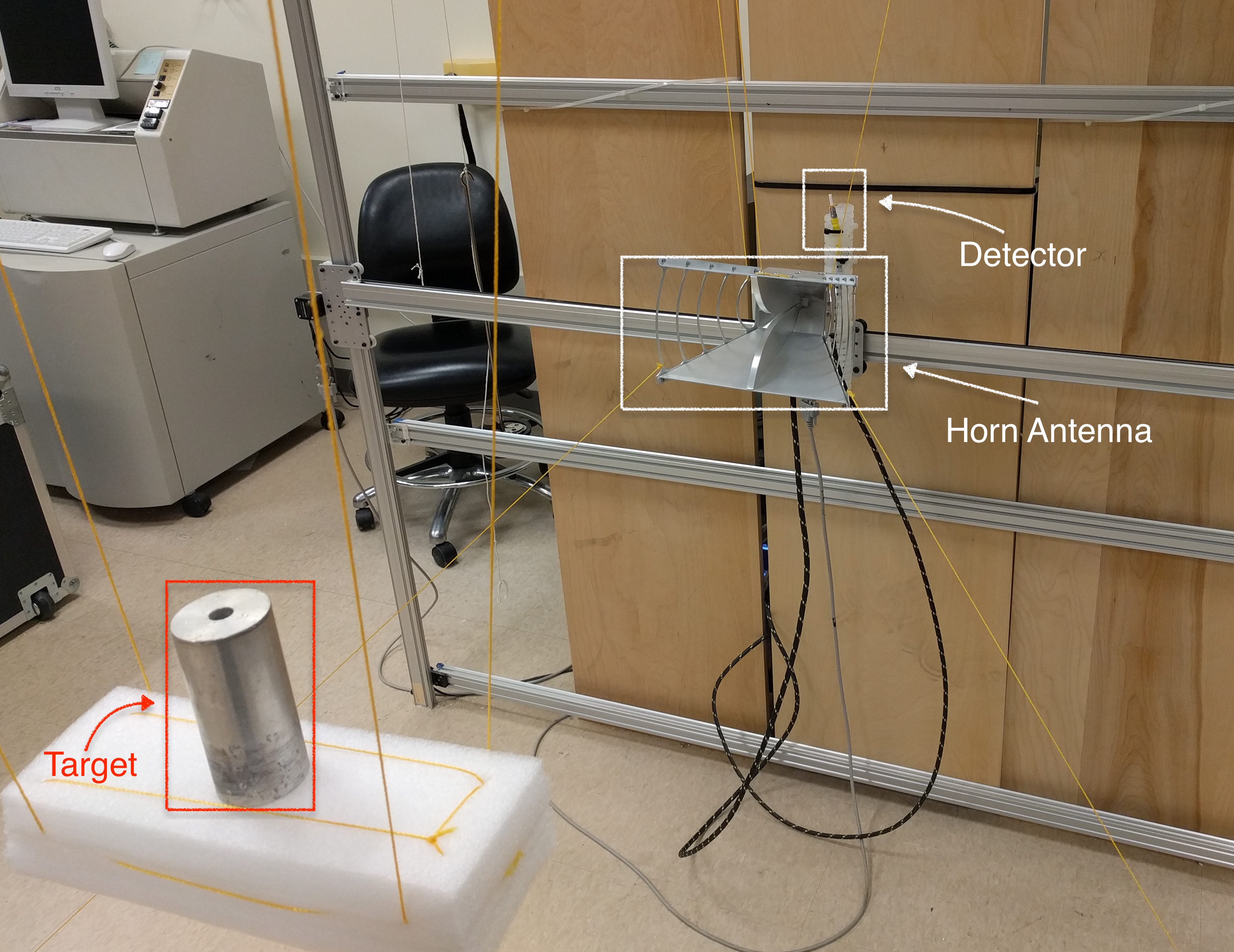
(a) A photograph of our experimental setup

(b) The schematic diagram of our setup

Figure 1: The experimental setup.

The measurement data has been collected in a regular room, see Figure 1. As mentioned in Introduction, keeping in mind our desired applications, we did not want to arrange a special anechoic chamber. On the measurement plane, which is a 1 m by 1 m area, we define that the $x$-axis and the $y$-axis are the horizontal and the vertical axis, respectively, while the $z$-axis is perpendicular to the measurement plane. The direction from the target, whose front face is positioned at $z=0$, to the measurement plane is the negative direction of the $z$-axis.

The source and receiver in the experiments are both from the same device, a 2 port Rohde $\&$ Schwarz vector network analyzer (VNA), connected by 2-meter Megaphase RF Killer Bee test cables. The broadband horn antenna and the collecting probe are both connected to the VNA. The antenna is positioned at a distance of about 75 cm from the target and 18 cm from the “wooden wall” of Figure 1(a), where the probe (i.e. detector) is located. For some technical reasons it was impossible to place the antenna behind that “wooden wall”. The VNA sends single frequency signals at frequencies ranging from 1 GHz to 10 GHz via the horn antenna. Actually by design the signal is also emitted from the probe at the same time. This probe technically collects both emitted and reflected signals, more precisely their scattering parameters ($S$-parameters). However, in our setup, the reflection in the signal to each device is calibrated when the detector is at the central position ($x=y=0$), that is, the internal reflections are removed at the position where the signal is strongest. Nevertheless, the internal reflections are not calibrated at other locations of the detector, where the signals are supposed to be weak. Therefore, the measured data are supposed to be as close to just the wave scattered by the unknown target as possible. Still, the latter approximation is only accurate at the central position, where the calibration of the internal reflections was done. For the range of frequencies from 1 GHz to 10 GHz we collect the scattered wave at 300 frequency points uniformly distributed over that range.

To obtain the backscatter data on the measurement plane for a single incident wave, the experiment is repeated for different positions of the probe on the measurement plane, which is the above mentioned wooden wall. More precisely, the probe is uniformly moved over the scanning area with the step size 2 cm, that means a total of 2550 data points. We scale to dimensionless variables by considering ${\bf x}={\bf x}/(10\,\mathrm{cm})$ for the convenience in our numerical implementation. Therefore, from now on when we see, for example $0.75$ of length, this means $7.5$ cm. Let $\mathbf{E}=(E_{x},E_{y},E_{z})$ be the electric field. The component $E_{y}$, which is the voltage, was incident upon the medium and the backscatter signal of the same component was measured. Therefore, we denote $u({\bf x},k):=E_{y}({\bf x},k)$, where the function $u({\bf x},k)$ is the above discussed solution of the problem (1)–(3). As it is stated in section 4.2.2, our central frequency is 3.1 GHz which corresponds to the wavelength $\lambda=9.67$ cm. This means that the source/target distance was 7.75 $\lambda$. Since this distance is sufficiently large in terms of $\lambda$, we have treated the incident wave as a plane wave $E_{y,inc}=e^{ikz}$.

4.2 Data preprocessing

Due to a significant amount of noise involved in the measured data, there is a considerable mismatch between these data and the computationally simulated data, see Figure 2. Here are the main indicators for the significant noise in the measured data.

• The emitted signal propagates not only towards the target but also backwards to the measurement plane.

• The measured signals are not only from the targets but also from other objects located in the room. In addition, there were some metallic parts of our device placed behind the measurement plane. So, the signals are scattered by these parts and come back to the detectors. Furthermore, these signals are affected by WiFi signals.

• The horn antenna is placed between the measurement plane and the targets to be imaged, due to technical issues in the experimental setup. Hence, a part of the wave reflected by these targets arrives back to the antenna. It is then scattered by the antenna and the latter signal propagates to the probe. This causes some additional parasitic signals.

• There is a significant difference in scales of magnitudes of experimental and computationally simulated data. One of the reasons is that it is not clear how to mathematically model the power of the emitted source.

• Due to the instability of the emitted signal, the backscatter signal is unstable.

Therefore, to invert the measured data using the above numerical method, we develop here a new heuristic data preprocessing procedure. The goal of this procedure is twofold: (1) We sort of distill the signals reflected by targets of our interest from signals reflected by other objects and (2) We also make the experimental data look somehow similar to computationally simulated data. It consists of three main steps:

1. Data propagation. This step “moves” the data closer to the target. As a result, we obtain good estimates of $x,y$ coordinates of our targets. In addition, this step allows us to reduce the computational domain $\Omega$.

2. Selection of an interval of frequencies on which the propagated data are stable. Our observation is that this is a quite narrow interval.

3. Truncation and calibration of propagated data.

Next, the so preprocessed data are used as the input for the algorithm described in section 3.3.

(a) Real part of measured data

(b) Real part of simulated data

Figure 2: The measured data (left) and the simulated data (right) on the measurement plane ($xy$-plane) for $k=6.575$.

4.2.1 Data propagation

This is one of the most important steps in data preprocessing. Given the experimental data on the measurement plane, the data propagation process aims to approximate these data on a plane which is closer to the unknown target than the measurement plane. This process firstly reduces the computational domain for our algorithm and secondly makes the scattered field data to look more focused. In addition, we have observed in our computations that the data propagation process helps us separate our target signals from the unwanted signals, see the first paragraph of section 4.2. This important observation leads to suitable truncations for the data in the last step of the data preprocessing procedure.

The data propagation process is done using a well known method in optics called the angular spectrum representation, see, e.g., [26, Chapter 2]. We note that this technique has been successfully exploited in [31] for data preprocessing for the globally convergent method of [4].

We recall that the negative $z$-direction is from the target to the measurement plane. Denote by $g({\bf x},k)$ the experimental data defined on the measurement rectangle $P_{m}=\{{\bf x}:-5<x<5,-5<y<5,z=b\}$ of the plane $\left\{z=b\right\}$ and by $f({\bf x},k)$ its approximation on the propagated rectangle $P_{p}=\{{\bf x}:-5<x<5,-5<y<5,z=a\}$ of the plane $\left\{z=a\right\}.$ We set both functions $g$ and $f$ to be equal to zero on those parts of corresponding planes $\left\{z=b\right\}$ and $\left\{z=a\right\}$ which are outside of those rectangles. Abusing notations a little bit, we call below sets $P_{m}$ and $P_{p}$ “measurement plane” and “propagated plane” respectively. We have $b<a<0$ since $P_{p}$ is closer to the target than $P_{m}$. Using the method of the angular spectrum representation, we obtain

$$f(x,y,a,k)=\frac{1}{2\pi}\iint_{k_{x}^{2}+k_{y}^{2}<k^{2}}\hat{g}(k_{x},k_{y},k)e^{-i[k_{x}x+k_{y}y-k_{z}(a-b)]}\mathrm{d}k_{x}\mathrm{d}k_{y},$$ (23)

where

$$\hat{g}(k_{x},k_{y},k)=\frac{1}{2\pi}\iint_{\mathbb{R}^{2}}g(x,y,b,k)e^{i(k_{x}x+k_{y}y)}\mathrm{d}x\mathrm{d}y$$

and $k_{z}=(k^{2}-k_{x}^{2}-k_{y}^{2})^{1/2}$. The idea of the method is that we consider the Helmholtz equation satisfied by the total wave outside the scattering medium ($\varepsilon_{r}({\bf x})=1$). Then the Fourier transform with respect to $x$ and $y$ of the total field satisfies an ordinary differential equation in the $z$-direction. Together with the radiation condition and the boundary condition on the measurement plane $P_{m}$ one can solve the 1D problem and obtain the formula (23). We refer to [26, 31] for more details on the angular spectrum representation. In Figure 3(b) we present the absolute value of the experimental data on the propagated plane

$$P_{p}=\{{\bf x}:-5<x<5,-5<y<5,z=-0.75\},$$ (24)

computed by the formula (23) for the wavenumber $k=6.575$. Comparing Figure 3(a) and Figure 3(b), we can easily see that the focusing of the scattered field is considerably improved after data propagation. From now on it is important to note that we will be only interested in the propagated data instead of the measured one.

(a) Absolute value of measured data

(b) Absolute value of propagated data

Figure 3: We respectively display in (a) and (b) the absolute value of the measured and propagated data for $k=6.575$.

4.2.2 Choosing a stable frequency interval

By manually plotting the absolute value of the propagated data for all 300 frequencies from 1 GHz to 10 GHz, we observed that the variation of the focusing (as in Figure 5(b)) of the scattered field with respect to the frequency is continuous only on a small interval of frequencies centered at around 3.1 GHz. We call this interval a stable frequency interval, which is essential for the input data for our numerical method. Equivalently, in the numerical implementation this stable frequency interval determines the corresponding small interval $[\underline{k},\overline{k}]$ for the wavenumbers that is used in our theoretical setting. We remark that this phenomenon does not exist for the computationally simulated data since the propagated field focusing varies smoothly on any interval of frequencies. The latter is one of the significant discrepancies between the simulated data and the measured data. The stable frequency interval can also be roughly estimated in Figure 4, where we plot the absolute value of the propagated data, which is written as a matrix of $300\times 2550$. The stable interval of frequencies from Figure 4 is $[2.98,3.19]$ GHz, which implies that $[\underline{k},\overline{k}]=\left[6.25,6.70\right]$. We observed that the lower and upper bounds of such intervals differ only very slightly for the data from different targets considered in this paper.

From now on, by using $[\underline{k},\overline{k}]$ we understand that this wavenumber interval corresponds to a small interval of frequencies around 3.1 GHz, which is determined from the procedure in this section.

Figure 4: The absolute value of the experimental data after propagation for all frequencies ranging from 1 GHz to 10 GHz.

4.2.3 Truncation and calibration of propagated data

We know from section 4.2.2 that the focusing of the propagated data changes continuously on $[\underline{k},\overline{k}]$. However, the behavior of the absolute value of the propagated data on this interval of wavenumbers is still not close enough to those in simulations. Indeed, we observed that after data propagation the magnitude of the simulated data has a clear peak at the $xy$-location of the target for all frequencies, see Figure 5(b). For the propagated data, although its magnitude always attains the global maximum at the $xy$-location of the target for all $k\in[\underline{k},\overline{k}]$, it does not really have a clear peak as in simulations due to local maxima at other regions of the propagated plane, see Figure 3(b). However, those latter local maxima are not located at the same locations for different frequencies. On the other hand the global maximum is located at the same place for all $k\in[\underline{k},\overline{k}]$. From this important observation we guess that the $xy$-location of the target should be actually in some small neighborhood of the point where the propagated data attains its global maximum.

To make the propagated data look more similar to those in simulations we truncate those by taking the points for which its magnitude is greater than or equal to $80\%$ of its maximum value, and setting the rest to be zero. In other words, for each $k\in[\underline{k},\overline{k}]$ we replace the function $f(x,y,a,k)$ with the function $\widetilde{f}(x,y,a,k)$ where

$$\widetilde{f}(x,y,a,k)=\begin{cases}f(x,y,a,k),&\text{ if }|f(x,y,a,k)|\geq 0.8\max_{x,y}|f(x,y,a,k)|,\\ 0,&\text{ otherwise.}\end{cases}$$ (25)

After that we smooth the function $\widetilde{f}(x,y,a,k)$ by a Gaussian filter and obtain the function $\widetilde{f}_{smth}(x,y,a,k)$. More precisely, we use the smoothing function smooth3 in Matlab with the Gaussian option. This is done for all values of $k\in[\underline{k},\overline{k}]$. We display in Figure 5 the propagated data after this procedure for $k=6.575$. It can be seen that the behavior of the absolute value of these processed data looks more similar to that of simulated data. The results are similar for other wavenumbers $k$ in $[\underline{k},\overline{k}]$.

We are now at the last step of data preprocessing called data calibration. This process is to scale the amplitude of the measured data to the same scaling as in our simulations, since the experimental data and simulated data usually have quite different amplitudes. For example, in Figure 5, we can see that the maximal value of the absolute value of measured data is about 0.0065, while this value is about 0.4 for the simulated data. To do the scaling, we need the so-called calibration factor. For estimating the calibration factor, we use the measured data of a single calibrating object whose location, shape, size, and dielectric constant are known. The word “single” is important here to ensure that the calibration procedure is unbiased, which means that we are supposed to know such information for only the calibrating object.

For $k\in[\underline{k},\overline{k}]$, where $\underline{k}$ and $\overline{k}$ are chosen from the process of choosing a stable frequency interval of section 4.2.2, let $U_{cal.obj}^{sim}({\bf x},k)$ and $U_{cal.obj}^{exp}({\bf x},k)$ be the propagated data of the simulated and measured scattered field for the calibrating object, respectively. We define our calibration factor as

$$\quad A(k)=\frac{\max{|U_{cal.obj}^{sim}({\bf x},k)|}}{\max{\ |U_{cal.obj}^{exp}({\bf x},k)|}}.$$

It can be seen that the amplitude of $A(k)U_{cal.obj}^{exp}({\bf x},k)$ has the same scale to that of the simulated data. We use the calibration factor $A(k)$ for measured data of all other objects. More precisely, given the propagated and truncated scattered field data $\widetilde{f}_{smth}(x,y,a,k)$ obtained from (25), we consider $A(k)\widetilde{f}_{smth}(x,y,a,k)+e^{ikz}$ as the input for our algorithm in section 3.3. We emphasize that this calibration factor is computed using the geometrical and physical information of only a single object: the calibrating object.

(a) Propagated data after truncation

(b) Propagated data in simulation

Figure 5: The absolute value of the propagated data after truncation and the propagated data in simulation for $k=6.575$.

5 Numerical implementation and reconstruction results

We describe in this section some details of the numerical implementation and present the reconstruction results for our experimental data using the globally convergent algorithm. We have collected experimental data for five objects. So, we test here these five data sets. Each data set corresponds to a single scattering object, numbered from 1 to 5, see Table 1. Object 1 (a piece of yellow pine) is chosen as our calibrating object.

Table 1: Scattering objects

Object ID	Name of the object
1	A piece of yellow pine
2	A piece of wet wood
3	A geode
4	A tennis ball
5	A baseball

5.1 Some computational details

In our numerical implementation the front face of the target is positioned at $\{z=0\}$. We consider the domain $\Omega$ as

$$\Omega=(-2.5,2.5)\times(-2.5,2.5)\times(-0.75,4.25).$$

Here we propagate all the measured data to the rectangle $P_{p}$ located on the plane $\{z=-0.75\}$ and search for the unknown targets in the range $(-0.75,1)$ of the $z$-direction. This search range is motivated by both: similar ranges that have been used in [30, 31] and our desired applications for detection of hidden explosives. Indeed, $z\in(-0.75,1)$ means that the linear size of the target in the $z$-direction does not exceed 17.5 cm. It is well-known that typical linear size of antipersonnel mines and IEDs are between 5 cm and 15 cm. We note that the larger range $(-0.75,4.25)$ is considered for the goal of completing the backscatter data in the next section. Also in the $xy$-plane we restrict ourselves to the smaller area $(-2.5,2.5)^{2}$ than the original measurement one $(-5,5)^{2}$. The main reason comes from the observation that the truncated data is zero outside of the area $(-2.5,2.5)^{2}$, see Figure 5, and does not contribute to the reconstruction process. This restriction helps us reduce our computational domain.

To solve the Lippmann-Schwinger integral equation (6), we use a spectral method developed in [21, 32]. This method exploits a periodization technique of the integral equation introduced by G. Vainikko, which enables the use of the fast Fourier transform and a simple numerical implementation. We use this method to find the solution in a box containing the support of the function $\varepsilon_{r}-1$. The solution in the complement of the box in $\Omega$ is then computed by the integration in (6). We solve the boundary value problem (16)–(17) by a finite element method. More precisely, we use FreeFem++ [15], a standard software designed with a focus on solving partial differential equations using finite element methods. We refer to www.freefem.org for more information about FreeFem++.

We observed from data preprocessing that the location of a target in the $xy$-plane can be roughly estimated from the propagated data. Indeed, we define $\Omega_{T}$ as

$$\Omega_{T}=\left\{(x,y):|\widetilde{f}_{smth}(x,y,-0.75,\widetilde{k})|>0.7\max|\widetilde{f}_{smth}(x,y,-0.75,\widetilde{k})|\right\}\subset P_{p},$$

where $\widetilde{f}_{smth}(x,y,-0.75,\widetilde{k})$ is the propagated data after the truncation procedure in section 4.2.3 and $\widetilde{k}$ is the wavenumber corresponding to the frequency 3.1 GHz. Note that for each target $|\widetilde{f}_{smth}(x,y,-0.75,k)|$ has a positive peak whose location is the same for all $k\in[\underline{k},\overline{k}]$, see Figure 5. The truncation value 0.7 was chosen based on trial-and-error tests on simulated and calibrating targets. We observed that $\Omega_{T}$ provides a reasonable approximation for the $xy$-location of a target. The same truncation was applied to all targets. Hence, it is not biased. Using $\Omega_{T}$ and the assumption that we seek for the target in $(-0.75,1)$ of the $z$-direction, the coefficient $\varepsilon_{rn,i}$ is truncated as follows

$$\varepsilon_{rn,i}({\bf x}):=\begin{cases}\max\left(|\varepsilon_{rn,i}({\bf x})|,1\right),&{\bf x}\in\Omega_{T}\times(-0.75,1),\\ 1,&\text{elsewhere}.\end{cases}$$

After that it is smoothed by smooth3 in Matlab with the Gaussian option as in data truncation. The so obtained $\varepsilon_{rn,i}$ is then used for solving the Lippmann-Schwinger equation in Algorithm 1.

Another important detail we would like to mention is a modification for approximating the data $\psi({\bf x},k)=\partial_{k}g({\bf x},k)/g({\bf x},k)$ on $\Gamma=\{{\bf x}\in\partial\Omega:z=-0.75\}$, where $g({\bf x},k)=A(k)\widetilde{f}_{smth}(x,y,-0.75,k)+e^{-0.75ik}$. First we calculated $\partial_{k}g({\bf x},k)$ using finite difference. The function $g({\bf x},k)$ is supposed to be as close to the total field as possible and $\psi({\bf x},k)$ should be smooth with respect to $k$. However, the variation of $\psi({\bf x},k)$ with respect to $k$ in the small interval $[\underline{k},\overline{k}]$ is actually not small, since the behavior of $g({\bf x},k)$ with respect to $k$ is not similar to that of the corresponding total field in simulations. The latter is one of discrepancies between simulated and propagated experimental data. We observe from simulations that, for each $k\in[\underline{k},\overline{k}]$, the absolute value of the function $\psi({\bf x},k)=\partial_{k}g({\bf x},k)/g({\bf x},k)$ on the propagated plane typically has a global minimum at the $xy$-location of the scatterer. Motivated by this observation, we approximate $\psi({\bf x},k)$ by $\widetilde{\psi}({\bf x},k)=\partial_{k}g({\bf x},k)/g({\bf x},k^{\ast})$, where for each $k$ we choose such a value $k^{\ast}\in[\underline{k},\overline{k}]$ for which $|\widetilde{\psi}({\bf x},k)|$ has a global minimum. However, we also observed that the choice of $k^{*}$ is independent of $k$. By doing so, we see that the variation of $\widetilde{\psi}({\bf x},k)$ in $k$ becomes small enough, when compared with those in simulations to be used in the algorithm.

5.2 Completing the backscatter data

We recall that only the backscatter signals were measured in our experiments. This means that after the above data preprocessing procedure, the function $g({\bf x},k)$ was known only on the side $\Gamma=\{\mathbf{x}\in\partial\Omega:z=-0.75\}$ of the domain $\Omega$. As in [30, 19], we replace the missing data on the other parts of $\Omega$ by the corresponding solution of the forward problem in the homogeneous medium, where $\varepsilon_{r}({\bf x})=1$. In other words, in our computation, the function $g({\bf x},k)$ is extended on the entire boundary $\partial\Omega$ as

$$g({\bf x},k):=\begin{cases}g({\bf x},k),&{\bf x}\in\Gamma,\\ e^{ikz},&{\bf x}\in\partial\Omega\setminus\Gamma.\end{cases}$$ (26)

We remark that data completion methods are widely used for inverse problems with incomplete data. The data completion (26) is a heuristic technique relying on the successful experiences of our group when working with globally convergent methods for experimental data, see [30, 5]. Other data completion methods may also be applied.

5.3 The stopping criteria and choosing the final result

Now we introduce the rules for stopping the iterations and choosing the final result for our Algorithm 1 relying on the content of the convergence theorem of [19] and trial-and-error testing for simulated data. Indeed, the global convergence theorem 7.1 of [19] only claims that functions $\varepsilon_{rn,i}$ are located in a sufficiently small neighborhood of the true solution if the number of iterations is not too large. But this theorem does not claim that these functions tend to the exact solution, also see theorem 2.9.4 in [4] and theorem 5.1 in [5]. This implies that the stopping criteria should be chosen computationally.

We have two stopping criteria: one for the inner iterations and the second one for the outer iterations. Before stating those criteria precisely we need some definitions. Denote by $e_{n,i}$ the relative error between the two computed coefficients corresponding to two consecutive inner iterations of the $n$-th outer iteration. That means

$$e_{n,i}=\frac{\|\varepsilon_{rn,i}-\varepsilon_{rn,i-1}\|_{L^{2}(\Omega)}}{\|\varepsilon_{rn,i-1}\|_{L^{2}(\Omega)}},\quad\text{for }i=2,3,\dots$$

Consider the $n$-th and $(n+1)$-th outer iterations which contain $I_{1}$ and $I_{2}$ inner iterations, respectively. We define the sequence of relative errors associated to these two outer iterations as

$$e_{n,2},\dots,e_{n,I_{1}},\widetilde{e}_{n+1,1},e_{n+1,2},\dots,e_{n+1,I_{2}},$$ (27)

where

$$\widetilde{e}_{n+1,1}=\frac{\|\varepsilon_{rn+1,1}-\varepsilon_{rn,I_{1}}\|_{L^{2}(\Omega)}}{\|\varepsilon_{rn,I_{1}}\|_{L^{2}(\Omega)}}.$$

The inner iterations with respect to $i$ of the $n$-th outer iteration in the algorithm 1 are stopped when either $e_{n,2}<10^{-6}$ or $i=3$. Note that this rule is similar to the one used for “Test 2” in [30], where the maximal number of inner iterations is set up to be 5. During our numerical experiments we observed that the reconstruction results are essentially the same when we use either 3 or 5 for the maximal number of inner iterations.

Concerning the outer iterations with respect to $n$ in Algorithm 1, it can be seen from the stopping rule for the inner iterations that each outer iteration consists of at least 2 and at most 3 inner iterations. Equivalently, the error sequence (27) has at least 3 and at most 5 elements. We stop the outer iterations if there are two consecutive outer iterations for which their error sequence (27) has three consecutive elements less than or equal to $5\times 10^{-4}$. We emphasize again that we have no rigorous justification for these stopping rules; they rely on the content of the convergence theorem [19] and trial-and-error testing for simulated data.

We choose the final result for $\varepsilon_{r}({\bf x})$ by taking the average of its approximations $\varepsilon_{rn,i}({\bf x})$ corresponding to the relative errors in (27) that meet the stopping criterion for outer iterations. The computed dielectric constant is determined as the maximal value of the computed $\varepsilon_{r}({\bf x})$. We have observed in our numerical studies that we need no more than five outer iterations to obtain the final result.

5.4 Reconstruction results

We present in Table 2 the reconstruction results for the dielectric constant of the scattering objects under consideration. The second column of the table represents the dielectric constants at 3 GHz of the scattering objects, independently measured by physicists from the Department of Physics and Optical Science at the University of North Carolina Charlotte (M. A. Fiddy and S. Kitchin). The percent number in the brackets is the error in the measurement given by the standard deviation. The measured relative permittivity of object 5 (a baseball) was not available due to some technical issues.

Our reconstruction results and their relative errors compared with measured dielectric constants are in the last two columns of the table. One can observe a good accuracy for our reconstructions: only a few percent. The dielectric constant of object 2 (wet wood) is relatively high which leads to the worst error case in computations, as anticipated. We have obtained best errors in objects 1 and 3. Note that object 1 is the calibrating object. We also observe that the computational error in object 4 is 2.5 times less than its measurement error. The computational error does not exceed a few percent in all four cases, just as in [4, 30, 31].

Table 2: Measured and computed dielectric constant of the targets

Obj. ID	Measured $\varepsilon_{r}$ (std. dev.)	Computed $\varepsilon_{r}$	Relative error
1	5.30 (1.6%)	5.44	2.6%
2	8.48 (4.9%)	7.60	10.3%
3	5.44 (1.1%)	5.55	2.0%
4	3.80 (13.0%)	4.00	5.2%
5	not available	4.76	n/a

We display in Figures 6 and 7 the 3D-visualizations of exact and reconstructed geometry of the first four targets using isosurface in Matlab. We do not display the image for object 5, which is similar to that of object 4, since both are spherically shaped. In the isosurface plotting the isovalue was chosen to be 50% of the maximal value of the computed $\varepsilon_{r}$. This choice is simply based on the calibrating object and is applied to all other objects. From the figures we can see that locations of the targets are well-reconstructed. It can also be seen that although the shape reconstruction of targets is in general not very good, the results for spherical shaped objects 3 and 4 seem to be better than those of rectangular prism ones (objects 1 and 2), which is reasonable.

6 Summary

We have presented in this paper the performance on a set of experimental data of the recently developed globally convergent numerical method [19] for a Coefficient Inverse Problems for the Helmholtz equation. This is a CIP with the backscatter multi-frequency data resulting from a single direction of the incident plane wave, i.e., this is a CIP with the minimal amount of measurement. The key advantage of this method over traditional locally convergent inversion techniques is that, under a reasonable mathematical assumption in section 3.4, it rigorously provides a good approximation for the exact coefficient without a priori knowledge of a small neighborhood of this coefficient.

Our data were intentionally collected under non-ideal conditions: to model the focus of our applications, which are detection and identification of explosive devices. Thus, our data are contaminated by a significant amount of noise. Denoising procedures are inapplicable here since our data have a rich content. Thus, we have developed a new heuristic data preprocessing procedure. The result of this procedure is used as the input for our algorithm of section 3.3. This procedure distills signals reflected by targets of our interest from parasitic signals and also makes the preprocessed data look similarly with the computationally simulated data. In particular, one can see from a comparison of Figures 3(a) and 3(b) that the data propagation step of this procedure indeed helps us separate the signal reflected by our targets from those scattered by all other objects in the room.

Table 2 shows that we come up with a good reconstruction accuracy of dielectric constants of targets with the errors not exceeding a few percent. One can also see from this table that our method can reconstruct relatively large inclusion/background contrasts, the case that is well known to be difficult for conventional least-squares approaches. Figures 6 and 7 show that locations of targets are also reconstructed with a good accuracy. This is achieved even though the data are highly noisy and we measured only the backscatter data associated with a single incident field.

(a) Exact location and shape of object 1

(b) Reconstruction result of object 1

(c) Exact location and shape of object 2

(d) Reconstruction result of object 2

Figure 6: 3D visualizations of exact (left) and reconstructed (right) geometry for objects 1 and 2.

(a) Exact location and shape of object 3

(b) Reconstruction result of object 3

(c) Exact location and shape of object 4

(d) Reconstruction result of object 4

Figure 7: 3D visualizations of exact (left) and reconstructed (right) geometry for objects 3 and 4.

References

- [1] A. D. Agaltsov and R. G. Novikov, Riemann-Hilbert problem approach for two-dimensional flow inverse scattering, J. Math. Phys., 55 (2014), p. 103502.
- [2] H. Ammari, Y. Chow, and J. Zou, Phased and phaseless domain reconstruction in inverse scattering problem via scattering coefficients, SIAM J. Appl. Math., 76 (2016), pp. 1000–1030.
- [3] H. Ammari and H. Kang, Reconstruction of Small Inhomogeneities From Boundary Measurements, vol. 1846 of Lecture Notes in Mathematics, Springer, 2004.
- [4] L. Beilina and M. V. Klibanov, Approximate Global Convergence and Adaptivity for Coefficient Inverse Problems, Springer, New York, 2012.
- [5] L. Beilina and M. V. Klibanov, A new approximate mathematical model for global convergence for a coefficient inverse problem with backscattering data, J. Inverse Ill-Posed Probl., 20 (2012), pp. 513–565.
- [6] M. Born and E. Wolf, Principles of Optics: Electromagnetic Theory of Propagation, Interference and Diffraction of Light, Cambridge University Press, 7th ed., 1999.
- [7] A. L. Bukhgeim and M. V. Klibanov, Global uniqueness of a class of multidimensional inverse problems, Soviet Math. Dokl., 24 (1981), pp. 244–247.
- [8] M. Burger and S. Osher, A survey on level set methods for inverse problems and optimal design, European J. of Appl. Math., 16 (2005), pp. 263–301.
- [9] F. Cakoni and D. Colton, Qualitative Methods in Inverse Scattering Theory. An Introduction., Springer, Berlin, 2006.
- [10] G. Chavent, Nonlinear Least Squares for Inverse Problems: theoretical foundations and step-by-step guide for applications, Springer Netherlands, 2010.
- [11] D. Colton and A. Kirsch, A simple method for solving inverse scattering problems in the resonance region, Inverse Problems, 12 (1996), pp. 383–393.
- [12] D. L. Colton and R. Kress, Inverse acoustic and electromagnetic scattering theory, Springer, 2nd ed., 1998.
- [13] H. W. Engl, M. Hanke, and A. Neubauer, Regularization of inverse problems, Kluwer Acad. Publ., Dordrecht, Netherlands, 1996.
- [14] A. V. Goncharsky and S. Y. Romanov, Supercomputer technologies in inverse problems of ultrasound tomography, Inverse Problems, 29 (2013), p. 075004 (22pp).
- [15] F. Hecht, New development in FreeFem++, J. Numer. Math., 20 (2012), pp. 251–265.
- [16] S. I. Kabanikhin, K. K. Sabelfeld, N. S. Novikov, and M. A. Shishlenin, Numerical solution of the multidimensional gelfand-levitan equation, J. Inverse and Ill-Posed Problems, 23 (2015), pp. 439–450.
- [17] S. I. Kabanikhin, A. D. Satybaev, and M. A. Shishlenin, eds., Direct Methods for Solving Multidimensional Inverse Hyperbolic Problems, VSP, Utrecht, 2004.
- [18] A. Kirsch, Characterization of the shape of a scattering obstacle using the spectral data of the far field operator, Inverse Problems, 14 (1998), pp. 1489–1512.
- [19] M. V. Klibanov, H. Liu, and L. H. Nguyen, A globally convergent method for a 3-D inverse medium problem for the generalized Helmholtz equation, arxiv:1605.06147, (2016).
- [20] A. V. Kuzhuget, L. Beilina, M. V. Klibanov, A. Sullivan, L. Nguyen, and M. A. Fiddy, Blind backscattering experimental data collected in the field and an approximately globally convergent inverse algorithm, Inverse Problems, 28 (2012), p. 095007.
- [21] A. Lechleiter and D.-L. Nguyen, A trigonometric Galerkin method for volume integral equations arising in TM grating scattering, Adv. Comput. Math., 40 (2014), pp. 1–25.
- [22] J. Li, P. Li, H. Liu, and X. Liu, Recovering multiscale buried anomalies in a two-layered medium, Inverse Problems, 31 (2015), p. 105006.
- [23] J. Li, H. Liu, and Q. Wang, Enhanced multilevel linear sampling methods for inverse scattering problems, J. Comput. Phys., 257 (2014), pp. 554–571.
- [24] J. Li, H. Liu, and J. Zou, Locating multiple multiscale acoustic scatterers, SIAM Multiscale Model. Simul., 12 (2014), pp. 927–952.
- [25] R. G. Novikov, An iterative approach to non-overdetermined inverse scattering at fixed energy, Sbornik: Mathematics, 206 (2015), pp. 120–134.
- [26] L. Novotny and B. Hecht, Principles of Nano-Optics, Cambridge University Press, Cambridge, UK, 2nd ed., 2012.
- [27] M. Pastorino, Microwave Imaging, John Wiley & Sons, Hoboken, NJ, 2010.
- [28] H. Schubert and A. Kuznetsov, eds., Detection and Disposal of Improvised Explosives, Springer, Dordrecht, 2006.
- [29] M. Soumekh, Synthetic Aperture Radar Signal Processing, John Wiley & Son, New York, 1999.
- [30] N. T. Thành, L. Beilina, M. V. Klibanov, and M. A. Fiddy, Reconstruction of the refractive index from experimental backscattering data using a globally convergent method, SIAM J. Sci. Comput., 36 (2014), pp. 273–293.
- [31] N. T. Thành, L. Beilina, M. V. Klibanov, and M. A. Fiddy, Imaging of buried objects from experimental backscattering time dependent measurements using a globally convergent inverse algorithm, SIAM J. Imaging Sci., 8 (2015), pp. 757–786.
- [32] G. Vainikko, Fast solvers of the Lippmann-Schwinger equation, in Direct and Inverse Problems of Mathematical Physics, D. Newark, ed., Int. Soc. Anal. Appl. Comput. 5, Dordrecht, 2000, Kluwer, p. 423.
- [33] J. C. Weatherall, J. Barber, and B. T. Smith, Identifying explosives by dielectric properties obtained through wide-band millimeter-wave illumination, Proc. SPIE, 9462 (2015), p. 94620F.
- [34] M. Yamamoto, Carleman estimates for parabolic equations and applications, Inverse Problems, 25 (2009), p. 123013.