subsecref \newrefsubsecname = \RSsectxt \RS@ifundefinedthmref \newrefthmname = theorem \RS@ifundefinedlemref \newreflemname = lemma
Uncertainty in Monotone Co-Design Problems
Abstract
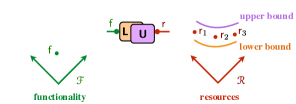
This work contributes to a compositional theory of “co-design” that allows to optimally design a robotic platform. In this framework, the user describes each subsystem as a monotone relation between “functionality” provided and “resources” required. These models can be easily composed to express the co-design constraints among different subsystems. The user then queries the model, to obtain the design with minimal resources usage, subject to a lower bound on the provided functionality. This paper concerns the introduction of uncertainty in the framework. Uncertainty has two roles: first, it allows to deal with limited knowledge of the models; second, it also can be used to generate consistent relaxations of a problem, as the computation requirements can be lowered, should the user accept some uncertainty in the answer.
Index Terms:
Co-Design; Optimization and Optimal Control; Formal Methods for RoboticsI Introduction
The design of a robotic platform involves the choice and configuration of many hardware and software subsystems (actuation, energetics, perception, control, …) in an harmonious entity. Because robotics is a young discipline, there is still little work towards obtaining systematic procedures to derive optimal designs. Therefore, robot design is a lengthly process based on empirical evaluation and trial and error.
The work presented here contributes to a theory of co-design [1, 2] that allows to optimally design a robotic platform based on formal models of its subsystems. The goal is to allow a designer to create better designs, faster. This work on “co-design” is related to and complementary to works that deal with “co-generation” (the ability of synthesizing hardware and software blueprints for entire robot platforms) [3, 4].
This paper describes the introduction of uncertainty in the theory developed so far. In this framework, the user defines “design problems” for each physical or logical subsystem. Each design problem (DP) is a relation between “functionality” provided and “resources” required by the component. The DPs can then composed in a graph, where each edge represents a “co-design constraint” between two DPs. The resulting class of problems is called Monotone Co-Design Problems (MCDPs).
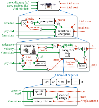
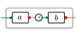
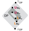
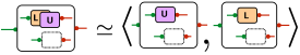
An example of MCDP is sketched in Fig. 1a. The design problem consists in finding an optimal configuration of a UAV, optimizing over actuators, sensors, processors, and batteries. In this simplified example, the functionality of the UAV is parameterized by three numbers: the distance to travel for each mission; the payload to transport; the number of missions to fly. The optimal design is defined as the one that satisfies the functionality constraints while using the minimal amount of resources (cost and mass). In the figure, the model is exploded to show how actuation and energetics are modeled. Perception is modeled as a relation between the velocity of the platform and the power required (the faster the platform, the more data needs to be processed). Actuation is modeled as a relation between lift and power/cost. Batteries are described by a relation between capacity and mass/cost. In this example, there are different battery technologies (LiPo, etc.), each specified by specific energy, specific cost, and lifetime, thus characterized by a different relation between capacity, number of missions and mass and cost. The interconnection between design problems describe the “co-design constraints”, which could be recursive: e.g., actuators must lift the batteries, the batteries must power the actuators. Cycles represent design problems that are coupled.
Once the model is defined, it can be queried to obtain the minimal solution in terms of resources — here, total cost and total mass. The output to the user is the Pareto front containing all non-dominated solutions. The corresponding optimization problem is, in general, nonconvex. Yet, with few assumptions, it is possible to obtain a systematic solution procedure, and show that there exists a dynamical system whose fixed point corresponds to the set of minimal solutions.
This paper describes how to add a notion of uncertainty in the MCDP framework. The model of uncertainty considered is interval uncertainty on arbitrary partial orders. For a partially ordered set (poset) , these are sets of the type . I will show how one can introduce this type of uncertainty in the MCDP framework by considering ordered pairs of design problems. Each pair describes lower and upper bounds for resources usage. These uncertain design problems (UDPs) can be composed using series, parallel, and feedback interconnection, just like their non-uncertain counterparts.
The output to the user is two Pareto fronts, describing the minimal resource consumptions in the best case and in the worst case according to the models specified. One or both the Pareto fronts can be empty, meaning that the problem does not have a feasible solution.
This is different from the usual formalization of “robust optimization” [5, 6], usually formulated as a “worst case” analysis, in which the uncertainty in the problem is described by a set of possible parameters, and the optimization problem is posed as finding the one design that is valid for all cases.
Uncertainty plays two roles: it can be used as a modeling tool, where the relations are uncertain because of our limited knowledge, and it can be used as a computational tool, in which we deliberately choose to consider uncertain relations as a relaxation of the problem, to reduce the computational load, while maintaining precise consistency guarantees. With these additions, the MCDP framework can describe even richer design problems and to efficiently solve them.
Paper organization
Section II and III summarize previous work. They give a formal definition of design problems (DPs) and their composition, called Monotone Co-Design Problems (MCDPs). Section IV through VI describe the notion of Uncertain Design Problem (UDP), the semantics of their interconnection, and the general theoretical results. Section VII describes three specific applications of the theory with numerical results. The supplementary materials (also available as [7]) include detailed models written in MCDPL and pointers to obtain the source code and a virtual machine for reproducing the experiments.
II Design Problems
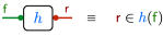
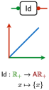
A design problem (DP) is a monotone relation between provided functionality and required resources. Functionality and resources are complete partial orders (CPO) [8], denoted and . The graphical representations uses nodes for DPs and green and red edges for functionality and resources.
Example 1.
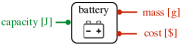
The first-order characterization of a battery is as a store of energy, in which the capacity [kWh] is the functionality (what the battery provides) and mass [kg] and cost [$] are resources (what the battery requires) (Fig. 2).
For a fixed functionality , the set of minimal resources in sufficient to perform the functionality might contain two or more elements that are incomparable with respect to . For example, in the case of a battery, one might consider different battery technologies that are incomparable in the mass/cost resource space.
A subset with “minimal”, “incomparable” elements is called “antichain”. This is the mathematical formalization of what is informally called a “Pareto front”.
Definition 2.
An antichain in a poset is a subset of such that no element of dominates another element: for all and , then .
Lemma 3.
Let be the set of antichains of . is a poset itself, with the partial order defined as
| (1) |
where “” denotes the upper closure of a set.
Definition 4.
Monotonicity implies that, if the functionality is increased, then the required resources increase as well.
III Monotone Co-Design Problems
A Monotone Co-Design Problem (MCDP) is a multigraph of DPs. An edge between a resource of a DP and a functionality of another denotes the partial order inequality constraint . Cycles and self-loops are allowed.
Example 5.
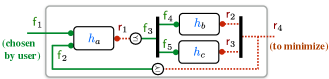
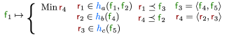
The MCDP in Fig. 4a is the interconnection of 3
DPs The semantics as an optimization
problem is shown in Fig. 4b. We will also
use an “algebraic” representation, shown in Fig. 4c,
and defined in Def. 6.
The functionality/resources parametrization is quite natural for many design engineering domains. Moreover, it allows for quantitative optimization, in contrast to qualitative modeling tools such as function structure diagrams [10]. All models considered may be nonlinear, in contrast to work such as Suh’s theory of axiomatic design [11].
III-A Algebraic definition
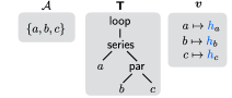
Some of the proofs rely on an algebraic representation of the graph. Series-parallel graphs (see, e.g., [12]) have widespread use in computer science. Here, we add a third operator to be able to represent loops. In the algebraic definition, the graph is a represented by a tree, where the leaves are the nodes, and the junctions are one of three operators (), as in Fig. 5. An equivalent construction for network processes is given in Stefanescu [13]. Equivalently, we are defining a symmetric traced monoidal category (see, e.g., [14] or [15] for an introduction); note that the operator is related to the “trace” operator, but not exactly equivalent, though they can be defined in terms of each other.


Let us use a standard definition of “operators”, “terms”, and “atoms” (see, e.g., [16, p.41]). Given a set of operators and a set of atoms , let be the set of all inductively defined expressions. For example, if the operator set contains only one operator with one argument, and there is only one atom , then the terms are
Definition 6 (Algebraic definition of Monotone Co-Design Problems).
An MCDP is a tuple , where:
-
1.
is any set of atoms, to be used as labels.
-
2.
The term in the algebra describes the structure of the graph:
-
3.
The valuation assigns a DP to each atom.
III-B Semantics of MCDPs
We can now define the semantics of an MCDP. The semantics is a function that, given an algebraic definition of an MCDP, returns a . Thanks to the algebraic definition, to define , we need to only define what happens in the base case (equation 2), and what happens for each operator (equations 3–5).
Definition 8 (Semantics of MCDP).
Given an MCDP in algebraic form , the semantics
is defined as follows:
(2)
(3)
(4)
(5)
The operators are defined in Def. 9–Def. 11. Please see [2, Section VI] for details about the interpretation of these operators and how they are derived.
The operator is a regular product in category theory: we are considering all possible combinations of resources required by and .
Definition 9 (Product operator ).
For two maps and , define
where is the product of two antichains.
The operator is similar to a convolution: fixed , one evaluates the resources , and for each , is evaluated. Then the minimal elements are selected.
Definition 10 (Series operator ).
For two maps and , if , define
The dagger operator is actually a standard operator used in domain theory (see, e.g., [9, II-2.29]).
Definition 11 (Loop operator ).
For a map , define
| (6) |
where is the least-fixed point operator, and is
III-C Solution of MCDPs
Def. 8 gives a way to evaluate the map for the graph, given the maps for the leaves. Following those instructions, we can compute , and thus find the minimal resources needed for the entire MCDP.
Example 12.
The MCDP in Fig. 4a is so small that we can do this explicitly. From Def. 8, we can compute the semantics as follows:
Substituting the definitions 9–11 above, one finds that with
The least fixed point equation can be solved using Kleene’s algorithm [8, CPO Fixpoint theorem I, 8.15]. A dynamical system that computes the set of solutions is given by
The limit is the set of minimal solutions, which might be an empty set if the problem is unfeasible for a particular value .
This dynamical system is a proper algorithm only if each step can be performed with bounded computation. An example in which this is not the case are relations that give an infinite number of solutions for each functionality. For example, the very first DP appearing in Fig. 1a corresponds to the relation for which there are infinite numbers of pairs for each value of travel distance. The machinery developed in this paper will make it possible to deal with these infinite-cardinality relations by relaxation.
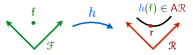
IV Uncertain Design Problems
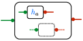
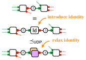
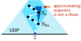
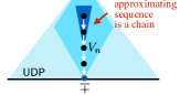
This section describes the notion of Uncertain DPs (UDPs). UDPs are an ordered pair of DPs that can be interpreted as upper and lower bounds for resource consumptions (Fig. 1b). We will be able to propagate this interval uncertainty through an arbitrary interconnection of DPs. The result presented to the user will be a pair of antichains — a lower and an upper bound for the resource consumption.
IV-A Partial order
Being able to provide both upper and lower bounds comes from the fact that in this framework everything is ordered – there is a poset of resources, lifted to posets of antichains, which is lifted to posets of DPs, and finally, to the poset of uncertain DPs.
The first step is defining a partial order on .
Definition 13 (Partial order ).
Consider two DPs . The DP precedes if it requires fewer resources for all functionality :
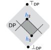
In this partial order, there is both a top and a bottom , defined as follows:
| (7) |
means that any functionality can be done with zero resources, and means that the problem is always infeasible (“the set of feasible resources is empty”).
IV-B Uncertain DPs (UDPs)
Definition 14 (Uncertain DPs).
An Uncertain DP (UDP) is a pair of DPs such that .
Definition 15 (Partial order ).
A UDP precedes another UDP if the interval is contained in the interval (Fig. 7):
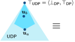
A DP is equivalent to a degenerate UDP .
A UDP is a bound for a DP if , or, equivalently, if .
V Interconnection of Uncertain Design Problems
We now define the interconnection of UDPs, in an equivalent way to the definition of MCDPs. The only difference between Def. 6 and Def. 16 below is that the valuation assigns to each atom an UDP, rather than a DP.
Definition 16 (Algebraic definition of UMCDPs).
An Uncertain MCDP (UMCDP) is a tuple , where is a set of atoms, is the algebraic representation of the graph, and is a valuation that assigns to each atom a UDP.
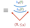
Next, the semantics of a UMCDP is defined as a map that computes the UDP. Def. 17 below is analogous to Def. 8.
Definition 17 (Semantics of UMCDPs).
Given an UMCDP , the semantics function computes a UDP
and it is recursively defined as follows:
VI Approximation results
The main result of this section is a relaxation result stated as Theorem 19 below. The following is an informal statement.
Informal statement
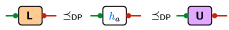
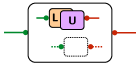
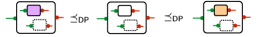
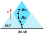
Consider an MCDP composed of many DPs, and call one (Fig. 8a). Suppose there exist two DPs , that bound the DP in the sense that (Fig. 8b). This can model either uncertainty in our knowledge of , or it can be a relaxation that we willingly introduce. The pair forms a UDP that can be plugged in the MCDP in place of (Fig. 8c). We will see that if we plug in only or separately in place of the original DP (Fig. 8d), we obtain a pair of MCDPs that form a UDP. Moreover, the solution of these two MCDPs are upper and lower bounds for the solution of the original MCDP (Fig. 8e). Therefore, we can propagate the uncertainty in the model to the uncertain in the solution. This result generalizes for any number of substitutions.
Formal statement
First, we define a partial order on the valuations. A valuation precedes another if it gives more information on each DP.
Definition 18 (Partial order on valuations).
For two valuations , say that if for all .
At this point, we have enough machinery in place that we can simply state the result as “the semantics is monotone in the valuation”.
Theorem 19 ( is monotone in the valuation).
If , then
Proof:
This follows easily from the definitions in Def. 18. As intermediate results, first prove that the lower bound is monotone in the valuation with respect to the order :
Then repeat the same reasoning for , to obtain:
These two together allow to conclude that is monotone with respect to the valuation with respect to the order :
∎
This result says that we can swap any DP in a MCDP with a UDP relaxation to obtain a UMCDP, which then we can solve to obtain inner and outer approximations to the solution of the original MCDP. This shows that considering interval uncertainty in the MCDP framework is easy because it reduces to solving a pair of problems instead of one. The rest of the paper consists of applications of this result.
VII Applications
This section shows three example applications of the theory:
-
1.
The first example deals with parametric uncertainty.
-
2.
The second example deals with the idea of relaxation of a scalar relation. This is equivalent to accepting a tolerance for a given variable, in exchange for reduced computation.
-
3.
The third example deals with the relaxation of relations with infinite cardinality. In particular it shows how one can obtain consistent estimates with a finite and prescribed amount of computation.
VII-A Parametric Uncertainty
To instantiate the model in Fig. 1a, we need to obtain numbers for energy density, specific cost, and operating life for all batteries technologies we want to examine. By browsing Wikipedia, one can find the figures in Table I.
| technology | energy density | specific cost | operating life | |
|---|---|---|---|---|
| [Wh/kg] | [Wh/$] | # cycles | ||
| NiMH | 100 | 3. | 41 | 500 |
| NiH2 | 45 | 10. | 50 | 20000 |
| LCO | 195 | 2. | 84 | 750 |
| LMO | 150 | 2. | 84 | 500 |
| NiCad | 30 | 7. | 50 | 500 |
| SLA | 30 | 7. | 00 | 500 |
| LiPo | 150 | 2. | 50 | 600 |
| LFP | 90 | 1. | 50 | 1500 |
Should we trust those figures? Fortunately, we can easily deal with possible mistrust by introducing uncertain DPs. Formally, we replace the DPs for energy density, specific cost, operating life in Fig. 1a with the corresponding Uncertain DPs with a configurable uncertainty. We can then solve the UDPs to obtain a lower bound and an upper bound to the solutions that can be presented to the user.
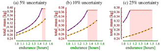
Fig. 9 shows the relation between the provided endurance and the minimal total mass required, when using uncertainty of , , on the numbers above. Each panel shows two curves: the lower bound (best case analysis) and the upper bound (worst case analysis). In some cases, the lower bound is feasible, but the upper bound is not. For example, in panel b, for 10% uncertainty, we can conclude that, notwithstanding the uncertainty, there exists a solution for endurance , while for values in , represented by the shaded area, we cannot conclude either the existence or nonexistence of a solution, because the lower bound is feasible, but the upper bound is not. This area of uncertainty depends on the parameter uncertainty injected (smaller for 5%, and larger for 25%).
VII-B Introducing Tolerances
Another application of the theory is the introduction of tolerances for any variable in the optimization problem. For example, one might not care about the variations of the battery mass below, say, . One can then introduce a uncertainty in the definition of the problem by adding a UDP hereby called “uncertain identity”.
VII-B1 The uncertain identity
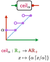
Let be a step size. Define and to be the floor and ceil with step size (Fig. 10). By construction,
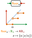
Let be the “uncertain identity”. For , it holds that
Therefore, the sequence is a descending chain that converges to as (Fig. 11).
VII-B2 Approximations in MCDP
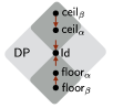
We can take any edge in an MCDP and apply this relaxation. Formally, we first introduce an identity and then relax it using (Fig. 12).
Mathematically, given an MCDP , we generate a UMCDP , where the new valuation agrees with except on a particular atom , which is replaced by the series of the original and the approximation :
Call the original and approximated DPs and :
Because (in the sense of Def. 18), Theorem 19 implies that
This means that we can solve and and obtain upper and lower bounds for . Furthermore, by varying , we can construct an approximating sequence of DPs whose solution will converge to the solution of the original MCDP.
Numerical results
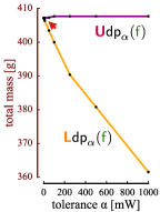
This procedure was applied to the example model in Fig. 1a by introducing a tolerance to the “power” variable for the actuation. The tolerance is chosen at logarithmic intervals between and . Fig. 13a shows the solutions of the minimal mass required for and , as a function of . Fig. 13a confirms the consistency results predicted by the theory. First, if the solutions for both and exist, then they are ordered (). Second, as decreases, the interval shrinks. Third, the bounds are consistent, in the sense that the solution for the original DP is always contained in the bounds.
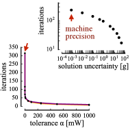
Next, it is interesting to consider the computational complexity. Fig. 13b shows the number of iterations as a function of the resolution , and the trade-off of the uncertainty of the solution and the computational resources spent. This shows that this approximation scheme is an effective way to reduce the computation load while maintaining a consistent estimate.
VII-C Relaxation for relations with antichains of infinite cardinality
Another way in which uncertain DPs can be used is to construct approximations of DPs that would be too expensive to solve exactly. For example, consider a relation like
| (8) |
which appears in the model in Fig. 1a. If we take these three quantities in (8) as belonging to , then, for each value of the travel distance, there are infinite pairs of that are feasible. On a computer, if the quantities are represented as floating point numbers, the combinations are properly not “infinite”, but, still, extremely large. We can avoid considering all combinations by creating a sequence of uncertain DPs that use finite and prescribed computation.
VII-C1 Relaxations for addition
Consider a monotone relation between some functionality and resources described by the constraint that (Fig. 14). For example, this could represent the case where there are two batteries providing the power , and we need to decide how much to allocate to the first () or the second ().
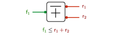
The formal definition of this constraint as an DP is
Note that, for each value , is a set of infinite cardinality. We will now define two sequences of relaxations for with a fixed number of solutions .
Using uniform sampling
We will first define a sequence of UDPs based on uniform sampling. Let consist of points sampled on the segment with extrema and . For , sample points on the segment and take the meet of successive points (Fig. 15).
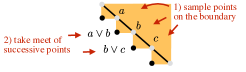
The first elements of the sequences are shown in Fig. 16. One can easily prove that , and thus is a relaxation of , in the sense that . Moreover, converges to as .
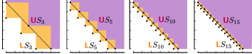
However, the convergence is not monotonic, in the sense that The situation can be represented graphically as in Fig. 19a. The sequence eventually converges to , but it is not a descending chain. This means that it is not true, in general, that the solution to the MCDP obtained by plugging in gives smaller bounds than .
Relaxation based on Van Der Corput sequence
We can easily create an approximation sequence that converges monotonically using Var Der Corput (VDC) sampling [17, Section 5.2]. Let be the VDC sequence of elements in the interval . The first elements of the VDC are . The sequence is guaranteed to satisfy and to minimize the “discrepancy”, a measure of uniform coverage.
The upper bound is defined as sampling the segment with extrema and using the VDC sequence:
The lower bound is defined by taking meets of successive points, according to the procedure in Fig. 15.
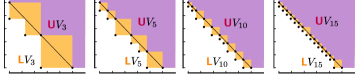
For this sequence, one can prove that not only , but also that the convergence is uniform, in the sense that The situation is represented graphically in Fig. 19b: the sequence is a descending chain that converges to .
VII-C2 Dual of multiplication
The case of multiplication can be treated analogously to the case of addition. By taking the logarithm, the inequality can be rewritten as So we can repeat the constructions done for addition. The VDC sequence are shown in Fig. 18.
VII-C3 Numerical example
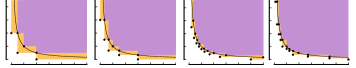
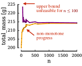
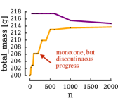
This relaxation strategy was applied to the relation in the MCDP in Fig. 1a. Thanks to the theory, we can obtain estimates of the solutions using bounded computation, even though that relation has infinite cardinality.
Fig. 19c shows the result using uniform sampling, and Fig. 19d shows the result using VDC sampling. As predicted by the theory, uniform sampling does not give monotone convergence, while VDC sampling does.
VIII Conclusions and future work
Monotone Co-Design Problems (MCDPs) provide a compositional theory of “co-design” that describes co-design constraints among different subsystems in a complex system, such as a robotic system.
This paper dealt with the introduction of uncertainty in the framework, specifically, interval uncertainty. Uncertainty can be used in two roles. First, it can be used to describe limited knowledge in the models. For example, in Section VII-A, we have seen how this can be applied to model mistrust about numbers from Wikipedia. Second, uncertainty allows to generate relaxations of the problem. We have seen two applications: introducing an allowed tolerance in one particular variable (Section VII-B), and dealing with relations with infinite cardinality using bounded computation resources (Section VII-C).
Future work includes strengthening these results. For example, we are not able to predict the resulting uncertainty in the solution before actually computing it; ideally, one would like to know how much computation is needed (measured by the number of points in the antichain approximation) for a given value of the uncertainty that the user can accept.
References
- [1] Andrea Censi “Monotone Co-Design Problems; or, everything is the same” In Proceedings of the American Control Conference (ACC), 2016
- [2] Andrea Censi “A Mathematical Theory of Co-Design” In CoRR abs/1512.08055, 2015 URL: http://arxiv.org/abs/1512.08055
- [3] A. M. Mehta, J. DelPreto, B. Shaya and D. Rus “Cogeneration of mechanical, electrical, and software designs for printable robots from structural specifications” In Proceedings of the IEEE/RSJ International Conference on Intelligent Robots and Systems (IROS), 2014, pp. 2892–2897 DOI: 10.1109/IROS.2014.6942960
- [4] Ankur M. Mehta et al. “Robot Creation from Functional Specifications” In The International Symposium on Robotics Research (ISRR), 2015
- [5] Dimitris Bertsimas, David B. Brown and Constantine Caramanis “Theory and Applications of Robust Optimization.” In SIAM Review 53.3, 2011, pp. 464–501 DOI: 10.1137/080734510
- [6] Aharon Ben-Tal, Laurent El Ghaoui and Arkadi Nemirovski “Robust Optimization” Walter de Gruyter GmbH, 2009 DOI: 10.1515/9781400831050
- [7] Andrea Censi “Handling Uncertainty in Monotone Co-Design Problems” Extended version on Arxiv with supplementary materials URL: http://tiny.cc/mcdp_uncertainty_extended
- [8] B.A. Davey and H.A. Priestley “Introduction to Lattices and Order” Cambridge University Press, 2002 DOI: 10.1017/cbo9780511809088
- [9] G. Gierz et al. “Continuous Lattices and Domains” Cambridge University Press, 2003 DOI: 10.1017/cbo9780511542725
- [10] Gerhard Pahl, W. Beitz, Jörg Feldhusen and Karl-Heinrich Grote “Engineering Design: A Systematic Approach” Springer, Hardcover, 2007
- [11] N.P. Suh “Axiomatic Design: Advances and Applications” Oxford University Press, 2001
- [12] R.J Duffin “Topology of series-parallel networks” In Journal of Mathematical Analysis and Applications 10.2 Elsevier BV, 1965, pp. 303–318 DOI: 10.1016/0022-247x(65)90125-3
- [13] Gheorghe Ştefănescu “Network Algebra” Springer Science + Business Media, 2000 DOI: 10.1007/978-1-4471-0479-7
- [14] André Joyal, Ross Street and Dominic Verity “Traced monoidal categories” In Math. Proc. Camb. Phil. Soc. 119.03 Cambridge University Press (CUP), 1996, pp. 447 DOI: 10.1017/s0305004100074338
- [15] David I. Spivak “Category Theory for the Sciences” MIT, 2014
- [16] Jarda Jezek “Universal Algebra”, 2008
- [17] Steven M. LaValle “Planning Algorithms” Cambridge University Press, Hardcover, 2006 URL: http://planning.cs.uiuc.edu/
Appendix A Appendix
A-A Proofs
A-A1 Proofs of well-formedness of 17
As some preliminary business, we need to prove that 17 is well formed, in the sense that the way the semantics function is defined, it returns a UDP for each argument. This is not obvious from 17.
For example, for , the definition gives values for and separately, without checking that
The following lemma provides the proof for that.
Lemma 20.
Proof:
Lemma 21.
.
Proof:
Lemma 22.
.
Proof:
Lemma 23.
.
Proof:
This follows from the fact that is monotone (27). ∎
A-A2 Monotonicity lemmas for DP
These lemmas are used in the proofs above.
Lemma 24.
is monotone on .
Proof:
In 10, is defined as follows for two maps and :
It is useful to decompose this expression as the composition of three maps:
where “” is the usual map composition, and and are defined as follows:
and
From the following facts:
-
•
is monotone.
-
•
is monotone in .
-
•
is monotone in each argument if the other argument is monotone.
Then the thesis follows. ∎
Lemma 25.
is monotone on .
Proof:
The definition of (9) is:
Because of symmetry, it suffices to prove that is monotone in the first argument, leaving the second fixed.
We need to prove that for any two DPs such that
| (12) |
and for any fixed , then
Let . Then we have that
Because of (LABEL:Ikno), we know that
So the thesis follows from proving that the product of antichains is monotone (26). ∎
Lemma 26.
The product of antichains is monotone.
Lemma 27.
is monotone on .
Proof:
Let . Then we can prove that . From the definition of (11), we have that
with defined as
The least fixed point operator is monotone, so we are left to check that the map
is monotone. That is the case, because if then
∎
A-A3 Monotonicity of semantics
Lemma 28 ( is monotone in the valuation).
Suppose that are two valuations for which it holds that . Then .
A-A4 Proof of the main result, 19
We restate the theorem.
Appendix B Software
B-A Source code
The implementation is available at the repository http://github.com/AndreaCensi/mcdp/, in the branch “uncertainty_sep16”.
B-B Virtual machine
A VMWare virtual machine is available to reproduce the experiments at the URL https://www.dropbox.com/sh/nfpnfgjh9hpcgvh/AACVZfdVXxMoVqTYiHWaOwHAa?dl=0.
To reproduce the figures, log in with user password “mcdp”/”mcdp”. Then execute the following commands:
[] $ cd ~/mcdp
$ source environment.sh
$ cd libraries/examples/uav_energetics/
droneD_complete_templates.mcdplib
$ make clean
$ make paper-figures
See pages - of mcdp_icra_uncertainty_models.pdf