Stochastic predator-prey dynamics of transposons in the human genome

Abstract

Transposable elements, or transposons, are DNA sequences that can jump from site to site in the genome during the life cycle of a cell, usually encoding the very enzymes which perform their excision. However, some transposons are parasitic, relying on the enzymes produced by the regular transposons. In this case, we show that a stochastic model, which takes into account the small copy numbers of the transposons in a cell, predicts noise-induced predator-prey oscillations with a characteristic time scale that is much longer than the cell replication time, indicating that the state of the predator-prey oscillator is stored in the genome and transmitted to successive generations. Our work demonstrates the important role of number fluctuations in the expression of mobile genetic elements, and shows explicitly how ecological concepts can be applied to the dynamics and fluctuations of living genomes.

Transposable elements (TE) McClintock (1950, 1953) or transposons are DNA sequences that can migrate from site to site in a host genome. These mobile genetic elements are found in all three domains of life, but especially compose a significant fraction of eukaryotic genomes, for example, occupying 45% of the human genomic sequence International Human Genome Sequencing Consortium (2001). Transposons are regarded as a major driver of adaptation and evolution Kazazian (2004), since they can induce both beneficial and deleterious transformations in the host genome, by inserting into encoding or regulation sequences, or causing misaligned pairing and unequal crossovers of chromosomes. In most cases, the modifications are disadvantageous to the host, for example causing hemophilia A in humans Dombroski et al. (1991). The activity of TEs has historically been observed through detailed population level assays, but recent measurements have demonstrated their activity in real time in living cells, using sophisticated fluorescence techniques Kim et al. (2016), quantifying in detail how the stochastic processes of excision are not purely random, but reflect a cell’s environment and genetic history. The interplay between transposon dynamics and replication, the cell’s genotype and phenotype and the interactions with the environment are all reminiscent of population dynamics of organisms within an ecosystem, and this perspective is one that we explore and quantify here.

The dynamics of TEs are complex, but can be conveniently separated into two types of edit operation on the host genome: copy-and-paste, and cut-and-paste Wicker et al. (2007). DNA transposons cut themselves out of the original site on the genome and later reintegrate at another site, thus performing a “cut-and-paste” operation which leaves the genome size invariant. Retrotransposons first transcribe into mRNA intermediates and then retrotranscribe to a new site on the genome sequence. This “copy-and-paste” dynamics leads to the growth of the genome size. Some transposons (autonomous) encode the very enzymes which perform their excision, while others are parasitic (non-autonomous), relying on the enzymes produced by the regular TEs.

Several theoretical approaches have been proposed to study the dynamics of transposons. Population genetics models Charlesworth and Charlesworth (1983); Charlesworth et al. (1994); Langley et al. (1983); Brookfield and Badge (1997); Le Rouzic and Capy (2006); Le Rouzic and Deceliere (2005) were first developed to describe the equilibrium distribution of transposons in a population. Recent development views the genome as an ecosystem, with genetic elements of different types playing the role of individuals from different species Brookfield (2005); Venner et al. (2009); Le Rouzic et al. (2007a, a, b); Serra et al. (2013); Linquist et al. (2015). In the case of non-autonomous transposons, a mean-field predator-prey type model describes their parasitic relationship with an autonomous transposon Le Rouzic et al. (2007a, b). However, these models do not account for the molecular level interactions between transposable elements and the dynamic behavior turns out to be sensitively dependent on these details. Furthermore, in a cell the copy number fluctuations are large, since the number of active (expressed) transposons is usually of order ten to a hundred Brouha et al. (2003). Thus, the next generation of transposon models needs to take into account molecular details and stochasticity.

The purpose of this Letter is to develop a minimal individual-level model based on the specific interaction mechanism between a pair of autonomous-non-autonomous transposons. We begin with a model of the interactions between the TEs, and then use techniques from statistical mechanics to derive stochastic differential equations McKane and Newman (2005). Our model predicts that number fluctuations generate persistent, noisy oscillations in the populations of the TEs, with a characteristic time scale that is much longer than the cell replication time, indicating that the state of the predator-prey oscillator is stored in the genome and transmitted to successive generations. Our work builds upon recent results that have shown how demographic stochasticity in ecosystems, where population size is integer-valued and locally finite, can lead to minimal models of persistent population cycles McKane and Newman (2005) or spatial patterns Butler and Goldenfeld (2009); Biancalani et al. (2010); Täuber (2012); Houchmandzadeh (2014); Fort (2013) without extra assumptions about the details of predation.

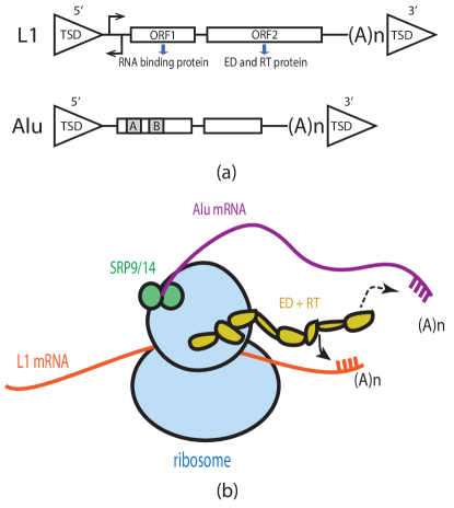
Figure 1: (Color online.) (a) shows the structure of L1 and Alu elements. L1 has a pol II promoter (the right-pointing arrow) and an antisense promoter (the left-pointing arrow) followed by two open reading frames (ORFs) encoding a RNA binding protein and a protein that consists of an endonuclease (ED) and a reverse transcriptase (RT), respectively. Alu is composed of two non-coding monomers, with the left one bearing A and B boxes (the shaded area in the figure) as the pol III promoter. L1 and Alu elements share similar poly-A tails and are both flanked by target site duplicates (TSDs). (b) shows the cis and trans effects of L1 elements. When an ED+RT protein is translated at the ribosome, it cis-preferentially binds with the L1 mRNA that codes it, indicated by the solid arrow. An Alu mRNA can bind with two signal recognition proteins SRP9 and SPR14, and then attach to the ribosome. The nascent ED+RT protein then can trans-bind to the Alu mRNA, which has a similar poly-A tail (indicated by the dashed arrow), presumably with a similar probability to binding to L1 mRNA.

Detailed model for transposon dynamics:- Retrotransposons consist of two subgroups: LTR-transposons that have a long terminal repeat (LTR) structure, and non-LTR transposons that do not Wicker et al. (2007). There are two types of non-LTR elements that show especially interesting interaction: the autonomous long interspersed nuclear elements (LINEs), and the non-autonomous short interspersed nuclear elements (SINEs) Singer (1982). In the human genome, the only active LINEs are LINE1 (L1) elements, which take up 17% of the entire genome International Human Genome Sequencing Consortium (2001). They help SINEs, such as Alu elements, to transpose by providing critical enzymes used in the copy-and-paste dynamics Mills et al. (2007). We take L1 and Alu elements in the human genome as an example of a LINE-SINE pair and build a model of their interaction.

When a protein is produced at a ribosome coded by an L1 mRNA, it tends to bind with that particular mRNA, presumably by recognizing its polyadenine (poly-A) tail Doucet et al. (2015), and later retrotranscribes it into the genome. This is known as the cis-preference of L1 elements Wei et al. (2001). However, if an Alu mRNA attaches to the same ribosome, then it can bind with the nascent protein by faking the L1 mRNA poly-A tail Boeke (1997). In this way, Alu elements steals the transposition machinery designed by L1 elements Weiner (2002); Dewannieux et al. (2003). This is known as the trans-effect of L1 elements Wei et al. (2001). The mechanism is sketched in Fig. 1(b).

Minimal model for transposon dynamics:- Based on the above detailed interaction, an individual level minimal model can be made, discarding all details about how proteins are made and how complexes are formed. The individual reactions are shown in Eq. (1), where $L$ stands for an active LINE, $S$ for an active SINE, and $R_{L}$ for the complex of the ribosome, LINE mRNA and nascent protein. Deactivated transposons do not participate in the transposition events and thus are excluded from the model.

An $L$ element encodes the complex $R_{L}$ at the rate $b_{R}$. The complex $R_{L}$ retro-transposes to produce a new $L$ element at the rate $b_{L}$, if there is no interruption. $S$ element hijacks the complex $R_{L}$ to duplicate itself at the rate $b_{S}/V$, where $V$ is the system size. The complex $R_{L}$ decays at the rate $d_{R}$. $L$ and $S$ elements are deactivated, at the rates $d_{L}$ and $d_{S}$, respectively. $\emptyset$ stands for null. The reactions for this minimal model, with the corresponding forward rates are as follows:

$$L \rightarrow L+R_{L}, b_{R}$$ (1a)

$$R_{L} \rightarrow L, b_{L}$$ (1b)

$$R_{L}+S \rightarrow 2S, b_{S}/V$$ (1c)

$$R_{L} \rightarrow\emptyset, d_{R}$$ (1d)

$$L \rightarrow\emptyset, d_{L}$$ (1e)

$$S \rightarrow\emptyset, d_{S}$$ (1f)

We assume the system is well mixed because mixing of reactants is faster, happening constantly within the cell lifetime, than the reactions.

We first use the Gillespie algorithm Gillespie (1976) to simulate the above reactions. Copy number vs time curves are plotted in Fig. 2. As shown in the figure, LINE and SINE copy numbers fluctuate around constant values, in the form of quasi-cycles. The circular envelope of the trajectory on the $L$-$S$ plane indicates a phase difference of roughly $\pi/2$, with SINE lagging LINE, supporting the identification of SINEs as predators on the LINEs.

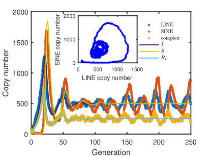
Figure 2: (Color online.) Results of a typical stochastic simulation with illustrative parameters $b_{R}=2$, $b_{L}=1$, $b_{S}=1$, $d_{R}=2$, $d_{L}=0.5$, $d_{S}=0.5$, and the system size $V=500$. The main figure shows the copy numbers of active LINEs, SINEs and ribosome/L-mRNA/protein complexes as a function of time, in the unit of a cell generation. Copy numbers fluctuate around constant values, demonstrating quasi-cycles with period $\sim 25$ generations. Solid lines are obtained by evolving the deterministic equations and show oscillatory decay toward steady values. Demographic noise induces quasi-cycles by constantly stimulating the deterministic oscillation mode. The inset shows the trajectory on the $L$-$S$ plane. The circular envelope indicates a phase difference of roughly $\pi/2$.

System size expansion:- Let the copy number concentrations of active LINEs, SINEs and complexes be $L$, $S$ and $R_{L}$ respectively. Then, with the system size being $V$, $VL$, $VS$ and $VR_{L}$ are equal to the actual copy numbers of the corresponding groups. The master equation about the probability $\mathcal{P}(L,S,R_{L})$ of the system being in the state $(L,S,R_{L})$ is written down as follows,

$$\frac{\mathrm{d}}{\mathrm{d}t}\mathcal{P}(L,S,R_{L})$$

$$= V\Bigl{\{}(\mathcal{E}_{R_{L}}^{-}-1)b_{R}L+(\mathcal{E}_{R_{L}}^{+}\mathcal{E}_{L}^{-}-1)b_{L}R_{L}$$

$$+(\mathcal{E}_{R_{L}}^{+}\mathcal{E}_{S}^{-}-1)b_{S}R_{L}S+(\mathcal{E}_{R_{L}}^{+}-1)d_{R}R_{L}$$

$$+(\mathcal{E}_{L}^{+}-1)d_{L}L+(\mathcal{E}_{S}^{+}-1)d_{S}S\Bigr{\}}\mathcal{P},$$ (2)

with the raising and lowering operators given by

$$\mathcal{E}_{X}^{\pm}f(X)\equiv f(\frac{N_{X}\pm 1}{V})\approx f(X)\pm\frac{1}{V}\partial_{X}f+\frac{1}{2V^{2}}\partial_{X}^{2}f,$$ (3)

where $f$ is an arbitrary function of the concentration $X$, and $X$ stands for $L$, $S$ or $R_{L}$.

Substituting the expansions of operators into the master Eq. (Stochastic predator-prey dynamics of transposons in the human genome), and saving terms up to order $O(V^{-1})$, we obtain a non-linear Fokker-Planck equation. The corresponding Langevin equations about concentrations $L$, $S$ and $R_{L}$ are nonlinear with multiplicative noises.

To obtain a set of linearized Langevin equations for concentration fluctuations, we perform the van Kampen’s system size expansion, separating concentrations into deterministic part, $\bar{L}$, $\bar{S}$ and $\bar{R}_{L}$, and stochastic part, $\xi$, $\eta$ and $\theta$, as follows.

$$L=\bar{L}+\frac{\xi}{\sqrt{V}},\quad S=\bar{S}+\frac{\eta}{\sqrt{V}},\quad R_{L}=\bar{R}_{L}+\frac{\theta}{\sqrt{V}}.$$ (4)

Writing

$$\Pi(\xi,\eta,\theta)\equiv\mathcal{P}(L,S,R_{L}),$$ (5)

we find that

$$\frac{\mathrm{d}}{\mathrm{d}t}\mathcal{P}=\partial_{t}\Pi-\sqrt{V}\frac{\mathrm{d}\bar{L}}{\mathrm{d}t}\partial_{\xi}\Pi-\sqrt{V}\frac{\mathrm{d}\bar{S}}{\mathrm{d}t}\partial_{\eta}\Pi-\sqrt{V}\frac{\mathrm{d}\bar{R}_{L}}{\mathrm{d}t}\partial_{\theta}\Pi.$$ (6)

Substituting the system size expansion expressions Eq. (4) into the nonlinear Fokker-Planck equation and matching orders of $V$, we obtain to $O(\sqrt{V})$

$$\frac{\mathrm{d}\bar{L}}{\mathrm{d}t} =b_{L}\bar{R}_{L}-d_{L}\bar{L},$$ (7a)

$$\frac{\mathrm{d}\bar{S}}{\mathrm{d}t} =b_{S}\bar{S}\bar{R}_{L}-d_{S}\bar{S},$$ (7b)

$$\frac{\mathrm{d}\bar{R}_{L}}{\mathrm{d}t} =b_{R}\bar{L}-b_{L}\bar{R}_{L}-b_{S}\bar{S}\bar{R}_{L}-d_{R}\bar{R}_{L}.$$ (7c)

These are the deterministic, or mean field, equations. The coexistence steady state, where $\bar{L}$, $\bar{S}$ and $\bar{R}_{L}$ are all non-zero, is always exponentially stable, according to linear stability analysis. We have verified numerically that the imaginary part of the linear stability matrix eigenvalues provides a reasonable estimate for the angular frequency of quasi-cycles. Specifically, for the parameters used to generate Fig. 2 and Fig. 3, the eigenvalue imaginary part is equal to $0.2330$, and agrees well with the Gillespie simulation value for the peak angular frequency, $0.23$ generation^-1, of the quasi-cycle power spectra shown in Fig. 3.

By matching $O(1)$ terms, we obtain the linearized Langevin equations for $\xi$, $\eta$ and $\theta$ using Ito’s Lemma Itô (1944):

$$\frac{\mathrm{d}\xi}{\mathrm{d}t} =b_{L}\theta-d_{L}\xi+r(t),$$ (8a)

$$\frac{\mathrm{d}\eta}{\mathrm{d}t} =b_{S}\bar{R}_{L}\eta+b_{S}\bar{S}\theta-d_{S}\eta+s(t),$$ (8b)

$$\frac{\mathrm{d}\theta}{\mathrm{d}t} =b_{R}\xi-b_{L}\theta-b_{S}\bar{R}_{L}\eta-b_{S}\bar{S}\theta-d_{R}\theta+h(t).$$ (8c)

$r(t)$, $s(t)$ and $h(t)$ are noises in $\xi$, $\eta$ and $\theta$, respectively. The correlations between these noises are given by

$$\langle h(t)h(t^{\prime})\rangle =\delta(t-t^{\prime})(b_{R}\bar{L}+b_{L}\bar{R}_{L}+b_{S}\bar{S}\bar{R}_{L}+d_{R}\bar{R}_{L}),$$ (9a)

$$\langle r(t)r(t^{\prime})\rangle =\delta(t-t^{\prime})(b_{L}\bar{R}_{L}+d_{L}\bar{L}),$$ (9b)

$$\langle s(t)s(t^{\prime})\rangle =\delta(t-t^{\prime})(b_{S}\bar{S}\bar{R}_{L}+d_{S}\bar{S}),$$ (9c)

$$\langle h(t)r(t^{\prime})\rangle =\delta(t-t^{\prime})(-b_{L}\bar{R}_{L}),$$ (9d)

$$\langle h(t)s(t^{\prime})\rangle =\delta(t-t^{\prime})(-b_{S}\bar{S}\bar{R}_{L}),$$ (9e)

$$\langle r(t)s(t^{\prime})\rangle =0.$$ (9f)

These Langevin equations describe the fluctuations of concentrations around the steady state values.

Persistent oscillations:- The power spectra $P_{\xi\xi}(\omega)$ and $P_{\eta\eta}(\omega)$ can be calculated by manipulating the Fourier transform of Eq. (8) and the correlations Eq. (9). The result is a complicated fraction, of which the numerator is a fourth order polynomial of $\omega$ and the denominator a sixth order polynomial of $\omega$. Asymptotically, the power spectra have a tail in the form of $\omega^{-2}$. Figure 3 shows a comparison between the power spectra obtained from simulation and the analytic calculation, which demonstrates a satisfactory agreement. This minimal model shows that the negative feedback of SINEs on LINE transposition rate results in a predator-prey like dynamics McKane and Newman (2005), with noise induced quasi-cycles.

Figure 3: (Color online.) Power spectra of the LINE and SINE concentration fluctuations. Circles stand for the power spectra obtained by averaging over 1000 replicates. Solid lines stand for the calculated spectra. The dash line is a reference function $\sim\omega^{-2}$. Parameters are $b_{R}=2$, $b_{L}=1$, $b_{S}=1$, $d_{R}=2$, $d_{L}=0.5$, $d_{S}=0.5$, $V=500$. The peak angular frequency is equal to $0.23$ generation^-1, corresponding to a period of $27$ generations. The straight tail, in log-log scale, has a slope of $-2$, indicating a $\omega^{-2}$ asymptotic behavior.

Estimation of parameters:- For the human genome, transposition rates of L1 and Alu elements measured by the mutation accumulation method are of order 1 in $O(10)\sim O(100)$ births Rosenberg et al. (2003); Huang et al. (2012); Cordaux et al. (2006). The deactivation rates have a lower limit set by the base pair point mutation rate, which is roughly $10^{-8}$ per base pair per generation Nachman and Crowell (2000); Roach et al. (2010). These rates seem to be too slow to generate any experimentally detectable dynamical behaviors. However, this estimate only accounts for fixed mutations that are not lethal, and thus underestimates the actual mutation rates. In a recent experiment Kim et al. (2016) on real-time transposition events in living bacterium cells, the actual transposition rate directly observed was $10^{3}$ times higher than that obtained by the mutation accumulation method. Moreover, the point mutation rate can be raised by a factor of $10^{2}$ by deactivating the base pair mismatch repair machinery Elez et al. (2010). Thus, for a single-cell experiment rather than a large population, the relevant estimate is: $b_{R}=2$, $b_{L}=1\times 10^{-2}$, $b_{S}=1\times 10^{-2}$, $d_{R}=1$, $d_{L}=1\times 10^{-2}$, $d_{S}=1\times 10^{-2}$, with units being generation^-1. The resultant quasi-cycle period should be roughly $1\times 10^{3}$ generations. Such oscillations could potentially be observed by integration of the LINE/SINE elements into a host microbial cell, E. coli for example, and using novel reporter techniques Kim et al. (2016); Kuhlman .

In conclusion, we have shown that the dynamics of transposons can fruitfully be analyzed using analogy to ecological models, equipped with tools from statistical physics. Our calculations predict the existence of potentially observable, persistent and noisy oscillations in the populations of active SINEs and LINEs.