Finite-size scaling study of dynamic critical phenomena in a vapor-liquid transition

Abstract

Via a combination of molecular dynamics (MD) simulations and finite-size scaling (FSS) analysis, we study dynamic critical phenomena for the vapor-liquid transition in a three dimensional Lennard-Jones system. The phase behavior of the model has been obtained via the Monte Carlo simulations. The transport properties, viz., the bulk viscosity and the thermal conductivity, are calculated via the Green-Kubo relations, by taking inputs from the MD simulations in the microcanonical ensemble. The critical singularities of these quantities are estimated via the FSS method. The results thus obtained are in nice agreement with the predictions of the dynamic renormalization group and mode-coupling theories.

I Introduction

Understanding of the anomalous behavior of various static and dynamic quantities, in the vicinity of the critical points 2MEFisher1 ; 2MEFisher2 ; 2MEFisher3 ; 2HEStanley ; 2PCHohenberg ; 2AOnuki1 ; 2VPrivman ; rev_sengers ; 2DPLandau ; 2MAnisimov ; 2LMistura ; 2HCBurstyn1 ; 2RAFerrell1 ; 2HCBurstyn2 ; 2RAFerrell2 ; 2GAOlchowy ; 2RFolk1 ; 2JLStrathmann ; 2AOnuki2 ; 2RFolk2 ; 2JZJustin ; 2HHao ; 2JKBhattacharjee1 ; 2JKBhattacharjee2 , is of fundamental importance. The critical behavior of the static quantities have been understood to a good extent via analytical theories, experiments and computer simulations 2MEFisher1 ; 2MEFisher2 ; 2MEFisher3 ; 2HEStanley ; 2AOnuki1 ; 2VPrivman ; 2DPLandau . On the other hand, the situation with respect to dynamics is relatively poor. Simulation studies, that helped achieving the objective for the static phenomena, gained momentum in the context of dynamic critical phenomena only recently 2KJagannathan1 ; 2KMeier ; 2KJagannathan2 ; 2AChen ; 2SKDas1 ; 2SKDas2 ; 2KDyer ; 2SRoy1 ; 2MGross ; 2SRoy2 ; 2SRoy3 ; 2SRoy4 ; 2SRoy5 ; 2JWMutoru . Such a status is despite the fact that adequate information on the equilibrium transport phenomena is very much essential for the understanding of even nonequilibrium phenomena like the kinetics of phase transitions 2AOnuki1 ; 2AJBray . For example, the crossovers and amplitudes in the growth-laws during phase transitions are often directly connected to the quantities like diffusivity and viscosity 2AJBray ; 2HFurukawa .

The static correlation length, $\xi$, diverges at the critical point 2HEStanley , i.e., $\xi\rightarrow\infty$ as the temperature $T\rightarrow T_{c}$, $T_{c}$ being the critical point value for the latter. As a result, various other static as well as dynamics quantities show singularities in approach to the criticality. These singularities are of power-law type, in terms of the reduced temperature ($\epsilon=|T-T_{c}|/T_{c}$), such as 2MEFisher1 ; 2MEFisher2 ; 2MEFisher3 ; 2HEStanley ; 2AOnuki1

$$\xi\sim\epsilon^{-\nu},~{}~{}\psi\sim\epsilon^{\beta},~{}~{}C\sim\epsilon^{-\alpha},~{}~{}\chi\sim\epsilon^{-\gamma}.$$ (1)

Here, $\psi$, $C$ and $\chi$ are the order-parameter, specific heat and susceptibility, respectively. Typically, singularities for various dynamic quantities, viz., mutual or thermal diffusivity ($D$), shear viscosity ($\eta$), bulk viscosity ($\zeta$), thermal conductivity ($\lambda$), etc., are expressed in terms of $\xi$ as 2PCHohenberg ; 2VPrivman ; 2MAnisimov

$$D\sim\xi^{-x_{D}},~{}~{}\eta\sim\xi^{x_{{}_{\eta}}},~{}~{}\zeta\sim\xi^{x_{{}_{\zeta}}},~{}~{}\lambda\sim\xi^{x_{{}_{\lambda}}}.$$ (2)

The static critical exponents do not depend upon the choice of material and the type of transition. In a particular dimension ($d$), if the interaction among the particles or spins are of same type, i.e., either of short or long range, and the order parameters have the same number of components, the exponents will have the same values, giving rise to well defined universality classes. For short range interactions with one component order-parameters, the exponents belong to the Ising universality class 2MEFisher1 ; 2MEFisher2 ; 2MEFisher3 ; 2HEStanley ; 2JZJustin . The universality of the critical exponents in statics, thus, is very robust, viz., paramagnetic to ferromagnetic, liquid-liquid, vapor-liquid transitions will all have the same set of exponent values depending upon the interaction range. Values of the above mentioned static exponents for the $d=3$ Ising class are 2JZJustin

$$\nu\simeq 0.63,~{}~{}\alpha\simeq 0.11,~{}~{}\beta\simeq 0.325,~{}~{}\gamma\simeq 1.239.$$ (3)

On the other hand, the universality of the dynamic exponents is considerably weaker. For example, the value of the exponent $z$, related to the longest relaxation time 2DPLandau

$$\tau\sim\xi^{z},$$ (4)

can vary depending upon the choice of statistical ensemble 2PCHohenberg ; 2AOnuki1 ; 2DPLandau . Nevertheless, the exponents for liquid-liquid and vapor-liquid transitions should be same, given by the fluid or model H universality class 2PCHohenberg ; 2AOnuki1 ; rev_sengers . The values of these exponents for this class are

$$x_{{}_{\lambda}}\simeq 0.902,~{}~{}x_{{}_{\eta}}\simeq 0.068,~{}~{}x_{{}_{\zeta}}\simeq 2.893,~{}~{}x_{{}_{D}}\simeq 1.068.$$ (5)

These numbers are obtained via the dynamic renormalization group and mode-coupling theoretical calculations and found to be in agreement with experiments 2PCHohenberg ; 2AOnuki1 ; 2MAnisimov ; 2LMistura ; 2HCBurstyn1 ; 2RAFerrell1 ; 2HCBurstyn2 ; 2RAFerrell2 ; 2GAOlchowy ; 2RFolk1 ; 2JLStrathmann ; 2AOnuki2 ; 2RFolk2 ; 2HHao ; 2JKBhattacharjee1 ; 2JKBhattacharjee2 ; rev_sengers . Like the static case, the dynamic exponents are also not all independent of each other, they follow certain scaling relations. E.g. starting from the generalized Stokes-Einstein-Sutherland relation 2HEStanley ; 2AOnuki1 ; 2JLStrathmann ; 2JPHansen

$$D=\frac{R_{D}k_{B}T}{6\pi\eta\xi},$$ (6)

$k_{B}$ being the Boltzmann constant and $R_{D}$ another universal constant 2JLStrathmann , one obtains 2HEStanley

$$x_{{}_{D}}=1+x_{{}_{\eta}}.$$ (7)

Unlike the static case, the computational estimation of the dynamic critical exponents started only recently, as mention above. In this work, we have presented simulation results for the critical dynamics of a three dimensional single component Lennard-Jones (LJ) fluid that exhibits vapor-liquid transition. We focus on the bulk viscosity and the thermal conductivity. There, of course, exist simulation studies on dynamics in vapor-liquid transitions 2KMeier ; 2AChen ; 2KDyer ; Sear1 . In fact, in some previous studies 2KMeier ; Sear1 both these transport properties were calculated in the vicinity of critical points. However, presumably due to computational difficulty with respect to the calculation of collective transport properties, corresponding critical exponents were not quantified in those 2KMeier ; Sear1 works. On the other hand, even though the critical behavior of the thermal diffusion constant was studied in Ref. 2AChen , the associated conductivity was not separately looked at.

For this purpose, we have performed molecular dynamics (MD) simulations and analyzed the results via appropriate application of the finite-size scaling (FSS) theory 2MEFisher4 . Prior to that, we have studied the phase behavior of the model by using the Gibbs ensemble Monte Carlo (GEMC) simulation method 2AZPanagiotopoulos as well as successive umbrella sampling technique Virnau1 in $NPT$ ensemble Wilding1 ; Panagio1 ($N$ and $P$ are the total number of particles and pressure, respectively). The critical temperature ($T_{c}$) and critical density ($\rho_{c}$) were estimated accurately via appropriate FSS analyses Wilding2 ; Kim1 ; Claud1 .

The rest of the paper has been organized as follows. In section II we have discussed the model and methodologies. The results are presented in section III. Finally, in section IV we have summarized our results.

II Model and Methods

As stated, we have considered a single component LJ fluid. In our model, a pair of particles, $i$ and $j$, separated by a distance $r$ ($=|\vec{r}_{i}-\vec{r}_{j}|$), interact via the potential 2MPAllen

$$U(r) = u(r)-u(r_{c})-(r-r_{c})\frac{du}{dr}\Big{|}_{r=r_{c}},~{}~{}\mbox{for}~{}r\leq r_{c}$$ (8)

$$= 0,~{}~{}\mbox{for}~{}r>r_{c},$$

where $r_{c}$ ($=2.5\sigma,\sigma$ being the particle diameter) is a cut-off distance, introduced to accelerate the computation. In Eq. (8), $u(r)$ is the standard LJ potential 2MPAllen ; 2DFrankel

$$u(r)=4\varepsilon\Big{[}\Big{(}\frac{\sigma}{r}\Big{)}^{12}-\Big{(}\frac{\sigma}{r}\Big{)}^{6}\Big{]},$$ (9)

with $\varepsilon$ being the interaction strength. For the sake of convenience we set $\sigma$ and $\varepsilon$ to unity. The last term in the first part of Eq. (8) was introduced to correct for the discontinuity in the force at $r=r_{c}$ that occurs after the cutting and shifting of the potential.

The GEMC simulations 2DFrankel ; 2AZPanagiotopoulos , for the study of the phase behavior of the model, were performed in two separate boxes, as discussed below. The total number of particles in and the total volume ($V$) of the two boxes were kept fixed, though the numbers of particles ($N_{1}$ and $N_{2}$) in as well as the volumes ($V_{1}$ and $V_{2}$) of the individual boxes were varied during the simulations. We considered three types of perturbations or trial moves, viz., particle displacement in each of the boxes, volume change of the individual boxes and particle transfer between the boxes. Thus, this is a combination of simulations in constant $NVT$, $NPT$ and $\mu_{c}VT$ ensembles, $\mu_{c}$ being the chemical potential. At a late time, one observes coexistence of the vapor phase (in one of the boxes) with the liquid phase (in the other box), if a simulation is performed at a temperature $T<T_{c}$. Thus, by running the simulations at different temperatures and obtaining the equilibrium densities ($\rho_{\alpha}=N_{\alpha}/V_{\alpha}$, $\alpha$ standing for liquid or vapor) of the individual phases, the whole phase diagram can be drawn, which, of course, will provide information about the critical temperature and critical density.

The phase diagram was also obtained via successive umbrella sampling Virnau1 MC simulations in $NPT$ ensemble Wilding1 ; Panagio1 . Like the grandcanonical case, the overall density fluctuates in this ensemble as well. While in the former the fluctuation is a result of particle addition and deletion moves, in the case of $NPT$ simulations the volume moves give rise to the fluctuation. The $NPT$ ensemble has advantage over the former when overall density is rather high. In the implementation of successive umbrella sampling technique, for overall density $\in[0,1]$, the corresponding volume range is divided into small windows. In each of these windows simulations were performed over long periods of time. For $T<T_{c}$, these simulations provide double-peak distribution for specific volume $v_{\rm sp}$ ($=V/N$). The peak at the smaller value of $v_{\rm sp}$, at a particular temperature, corresponds to a point on the liquid branch of the coexistence curve. The coexisting vapor density is given by the position of the peak at the higher value of $v_{\rm sp}$. While the coexistence curve data will be presented from the GEMC simulations, for the estimation of critical parameters, particularly $\rho_{c}$, we will rely on the simulations in $NPT$ ensemble. Here note that our results on the phase behavior are consistent with the data from the simulations in grandcanonical ensemble which are made available online NIST1 .

To study the transport properties we have performed MD simulations 2MPAllen ; 2DFrankel ; 2DCRapaport . There we first thermalize the systems, using the stochastic Andersen thermostat 2DFrankel , to generate the initial configurations. Finally, for the production runs we performed MD simulations in the microcanonical (constant $NVE$, $E$ being the total energy) ensemble that preserves hydrodynamics, essential for the calculations of transports in fluids 2DFrankel .

The transport quantities have been calculated by using the Green-Kubo (GK) formulae 2JPHansen ; 2MPAllen . The GK relations for the viscosities and the thermal conductivity are connected to the expressions 2JPHansen ; 2MPAllen

$$\mathcal{Y}=\frac{1}{k_{B}TV}\int_{0}^{t}dt^{\prime}<\sigma^{\prime}_{\mu s}(t^{\prime})\sigma^{\prime}_{\mu s}(0)>;~{}\mu,s\in[x,y,z],$$ (10)

and

$$\lambda=\frac{1}{k_{B}T^{2}V}\int_{0}^{t}dt^{\prime}<j^{s}_{T}(t)j^{s}_{T}(0)>;~{}s\in[x,y,z].$$ (11)

In Eq. (10), $\sigma^{\prime}_{\mu s}$ is related to the pressure tensor $\sigma_{\mu s}$, defined as

$$\sigma_{\mu s}=\sum_{i=1}^{N}\Big{[}m_{i}v_{i\mu}v_{is}+\sum_{j=i+1}^{N}(\mu_{i}-\mu_{j})F_{sj}\Big{]},$$ (12)

where $F_{sj}$ is the $s^{\mbox{th}}$ component of the force on the $j^{\mbox{th}}$ particle, $m_{i}$ is the mass of the $i^{\mbox{th}}$ particle (chosen to be equal to $m$ for all), $v_{i\mu(s)}$ is the $\mu(s)^{\mbox{th}}$ component of velocity for particle $i$ and $\mu_{i(j)}$ is the Cartesian coordinate for particle $i$($j$) along the $\mu$-axis. For the diagonal elements $\sigma^{\prime}_{\mu\mu}=\sigma_{\mu\mu}-<\sigma_{\mu\mu}>$ and $\mathcal{Y}=\zeta+4/3\eta$, whereas for the off-diagonal elements ($\sigma^{\prime}_{\mu s}=\sigma_{\mu s}$) $\mathcal{Y}=\eta$. In Eq. (11), $j_{T}^{s}$ is the thermal flux along any particular axis, defined as

$$j_{T}^{s}=\frac{1}{2}\sum_{i=1}^{N}v_{is}\Big{[}m|v_{i}|^{2}+\sum_{j\neq i}^{N}U(r)\Big{]}-\frac{1}{2}\sum_{i=1}^{N}\sum_{j\neq i}^{N}\vec{v}_{i}\cdot\vec{r}\frac{\partial U(r)}{\partial s},$$ (13)

where $v_{is}$ is the velocity component of the $i^{\mbox{th}}$ particle along $s$-axis. In $U(r)$ it is understood that the energy comes from the interaction between particles $i$ and $j$, vector distance between them being represented by $\vec{r}$. This justifies the summation over $j$ in the last equation.

All our simulations were performed in cubic systems of linear dimension $L$ and in the presence of periodic boundary conditions in all possible directions. In our MD simulations, time was measured in an LJ unit $t_{0}$ ($=\sqrt{m\sigma^{2}/\epsilon}$) and the integration time step was set to $dt=0.005t_{0}$. All the results related to transport properties are presented after averaging over 64 initial realizations. From here on, for the sake of convenience, we set $m$, $k_{B}$ and $t_{0}$ to unity. Note that the time in MC simulations is expressed in units of number of Monte Carlo steps (MCS). In the case of GEMC method, each step consists of $75\%$ displacement moves, $10\%$ volume moves, and $15\%$ particle transfer moves, of a total of $N$ trials. There was no particular order for the execution of these moves. Results for the coexistence curve are presented after averaging over 15 initial configurations.

III Results

A. Phase Behavior

In Fig. 1 we show the density profiles inside the two boxes, vs time, obtained from a typical run in the GEMC simulations 2AZPanagiotopoulos at $T=0.86$. For each of the studied temperatures, we started with density $\rho=0.3$, in each of the boxes. Gradually, the density in one of the boxes increases with time, while it decreases in the other box, if $T<T_{c}$. Finally, the densities inside both the boxes saturate and fluctuate around the mean values, as shown in this figure. The distribution of the densities, obtained from the profiles in Fig. 1, has been presented in Fig. 2. The appearance of the two peaks is expected (given that the profiles are well separated) and implies the coexistence of vapor and liquid phases. There the locations of the peaks correspond to the equilibrium density values of the vapor and liquid phases, for the studied temperature.

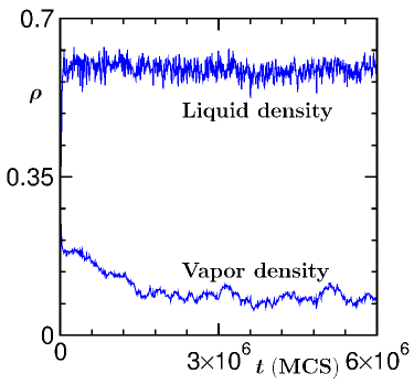
Figure 1: Density profiles inside the two boxes, during a Gibbs ensemble Monte Carlo run with $V=2\times 12^{3}$, are plotted vs time. The results correspond to $T=0.86$.

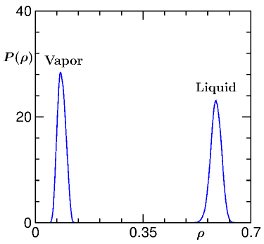
Figure 2: Plot of the density distribution function, $P(\rho)$, vs $\rho$, for the density profiles in Fig. 1.

In Fig. 3 (a) we have presented the phase diagram for the model, in the temperature vs density plane. We obtained this by plotting the equilibrium coexistence densities of the two phases at different temperatures. Accuracy of these results are checked by comparing with the ones obtained from umbrella sampling simulations in the $NPT$ ensemble. From this figure, it is clear that the value of the order-parameter $\psi$ ($=\rho_{\ell}-\rho_{v}$, $\rho_{\ell}$ and $\rho_{v}$ being respectively the liquid and vapor densities) is approaching zero with the increase of temperature. In Fig. 3 (a), we do not present data from temperatures very close to critical point, since they suffer from the finite-size effects. The finite-size effects were appropriately identified by comparing the results from different system sizes.

The values of $T_{c}$ and $\rho_{c}$ can be calculated by using the equations 2DFrankel

$$\psi=\rho_{\ell}-\rho_{v}=A(T-T_{c})^{\beta},$$ (14)

and

$$\rho_{d}=\frac{\rho_{\ell}+\rho_{v}}{2}=\rho_{c}+B(T-T_{c}),$$ (15)

where $A$ and $B$ are constants. For fitting the simulation data to Eq. (14), to obtain $T_{c}$, we choose $\beta=0.325$, which, as already mentioned, is its value for the $d=3$ Ising universality class. Since LJ potential is a short-range one, this value is expected. For the same reason, we will adopt the Ising value for $\nu$, while analyzing the transport properties. This exercise provides $T_{c}=0.939\pm 0.004$. This is in good agreement with a previous estimate via grandcanonical simulations, for the same model Errin1 .

Estimation of $\rho_{c}$, on the other hand, will suffer from error, if made via fitting to Eq. (15). This is because, Eq. (15) should contain additional terms in powers of ($T_{c}-T$), due to field mixing Wilding2 ; Kim1 ; Claud1 . Accurate finite-size scaling analyses Wilding2 ; Kim1 have been performed to extract $\rho_{c}$, that take care of these singularities. In some of these previous studies Wilding2 ; Errin1 only the term proportional to $\epsilon^{1-\alpha}$ have been considered. More recently, it has been stressed that the leading singularity Kim1 ; Claud1 is $\epsilon^{2\beta}$ and should be considered for more accurate estimation of $\rho_{c}$. Here we perform finite-size scaling analysis using this dominant contribution. For this exercise we have used data from NPT simulations at $T_{c}$. Recall that, like $L$ in the grandcanonical ensemble, here $N$ is kept fixed and we treat it as $L^{3}$.

In Fig. 3 (b) we show $\rho_{d}$ (upper curve) as a function of $L^{-2\beta/\nu(=1.032)}$. This scaling form comes from the fact that $\xi\sim L$ at $T_{c}$. Linear extrapolation of the data set to $L=\infty$ provides $\rho_{c}\simeq 0.317$. In this figure we have also included the mean value of $\rho$ ($\bar{\rho}$) (see lower plot), estimated from the inverse of the average specific volume. This also exhibits a linear behavior, extrapolation of which leads to $\rho_{c}\simeq 0.315$. From these exercises we take $\rho_{c}=0.316$. In Fig. 3 (a), the cross mark is the location of the critical point. The simulation data in this figure show nice consistency with the continuous line, which has the Ising behavior. Our estimation of $\rho_{c}$ is reasonably consistent with the previous Errin1 grandcanonical estimate ($0.320$). Little more than $1\%$ difference that exists may well be due to the fact that in this earlier work data were not analyzed by considering the leading singularity. Nevertheless, in view of this difference, we have calculated transport properties over a wide range of density, viz. $[0.31,0.32]$. While we will present results at our estimated value of $\rho_{c}$, outcomes from other densities will be mentioned in appropriate place.

Note that the values of $T_{c}$ and $\rho_{c}$ were estimated previously 2DFrankel ; Wilding2 for the vapor-liquid transitions in similar LJ models. However, those studies either used different values of $r_{c}$ or did not consider the term related to force correction. The difference in the numbers between our study and these previous ones are related to these facts. In fact, the cut-off dependence of the critical temperature is nicely demonstrated by Trokhymchuk and Alejandre Trokh1 . However, we cannot use the information from this work because of the force correction that we use.

Before proceeding to show the results for dynamics, in Fig. 4 we show the two-dimensional cross-sections of two typical equilibrium configurations at $T=0.95$ and $1.4$. Structural difference between the two snapshots is clearly visible. The one at $T=0.95$ shows density fluctuations at much larger length scale, implying critical enhancement in $\xi$. The values of $\xi$, as well as $\chi$, can be calculated from the density-density structure factors by fitting the small wave-vector data to the Ornstein-Zernike form 2HEStanley .

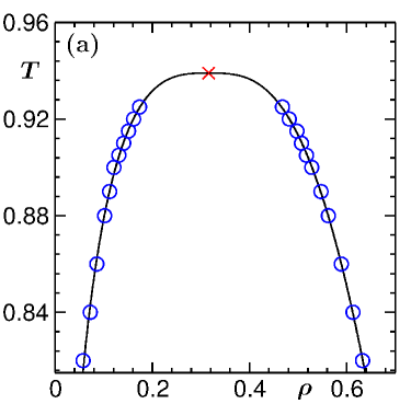
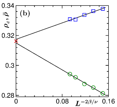
Figure 3: (a) Phase diagram of the 3D LJ fluid in the $T-\rho$ plane, obtained via the Gibbs ensemble Monte Carlo simulations. The cross mark in the figure is the location of the critical point. The continuous line represents the Ising critical behavior of the order parameter. The results correspond to $V=2\times 12^{3}$. (b) Demonstration of the estimation of $\rho_{c}$ via finite-size scaling analysis. Here we have plotted $\rho_{d}$ (upper curve) and $\bar{\rho}$ (lower curve), obtained from $NPT$ simulations at $T_{c}$, vs $L^{-2\beta/\nu}$

.

B. Dynamics

All the results for dynamics are presented from temperatures above the critical value, by fixing $\rho$ to $\rho_{c}$. In Fig. 5, we show the plots of $\zeta+\frac{4}{3}\eta$ and $\lambda$, vs time, as obtained from the GK formulas, at $T=0.96$, on a semi-log scale. We extract the final values for these quantities from the flat regions. From this figure it is clear that a transport quantity having higher critical exponent settles down to a flat plateau at a later time. This states about the difficulty of calculating a transport coefficient with strong critical divergence, like the bulk viscosity ($\zeta$), particularly close to $T_{c}$. The difficulty gets pronounced with the increase of system size, consideration of which is essential to avoid the finite-size effects in the critical vicinity. However, in our simulations we have used relatively small system sizes and relied on the FSS theory 2MEFisher4 for the estimation of the critical exponents.

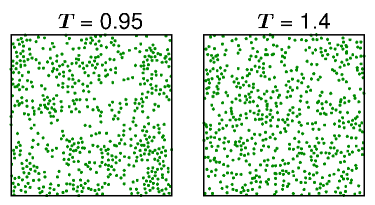
Figure 4: Two-dimensional slices of typical equilibrium configurations at $T=0.95$ and $1.4$. The dots mark the locations of the particles.

The temperature dependence of the bulk viscosity and the thermal conductivity, obtained from the plateaus of GK integrations, have been presented in Fig. 6 and Fig. 7, respectively. The enhancement in these quantities can be observed for both the presented system sizes, mentioned in the figure, close to $T_{c}$, represented by the dashed lines. Weaker enhancement for the smaller system, for both $\zeta$ and $\lambda$, signify finite-size effects.

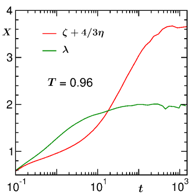
Figure 5: Plots of $X$ ($\zeta+\frac{4}{3}\eta,\lambda$) vs $t$, in a semi-log scale, at $T=0.96$, with $L=30$.

In Fig. 8 we show the plot of $\zeta$ vs $\epsilon$, using data from the larger system size that has been used in Fig. 6, on a log-log scale. We observe that the simulation data are in disagreement with the theoretically predicted solid line (having exponent $x_{{}_{\zeta}}\nu=1.82$). The reasons for the disagreement could be the finite-size effects as well as the presence of a background contribution 2HCBurstyn3 , the latter arising from small wavelength fluctuations. We observe similar disagreement for $\lambda$, presented in the inset of Fig. 8, for the same system size. These two serious issues, viz., finite-size effects and background contributions, have to be appropriately taken care of during the estimation of the critical exponents, along the line discussed below.

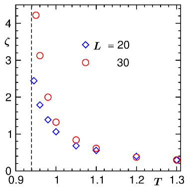
Figure 6: Plots of $\zeta$ vs $T$ for two different system sizes. Close to the critical point the error bars are of the order of the symbol sizes. The dashed line in the figure is the location of the critical temperature.

A quantity, say $X$, that exhibits singularity at the critical point, can be decomposed into two parts 2JLStrathmann ; 2SKDas1 ; 2SKDas2 ; 2HCBurstyn3 as

$$X=\Delta X(T)+X_{{}_{b}},$$ (16)

where $\Delta X(T)$ comes from the critical fluctuations and is strongly temperature dependent. On the other hand, $X_{b}$, the background, is only weakly temperature dependent and is often treated as a constant 2SKDas1 ; 2SKDas2 . This latter contribution should also be independent of the system size. The presence of such a term, particularly in computer simulations, where one works with finite systems, can lead to a misleading conclusion. To extract the correct critical divergence one needs to subtract it appropriately from the total value, such that

$$\Delta X(T)=X-X_{b}\sim\xi^{x},$$ (17)

where $x$ is the critical exponent for $X$. We have estimated $X_{b}$ by treating it as an adjustable parameter in the FSS analysis that we describe below. One might as well have aimed to obtain the background contributions from Fig. 8 by looking at the behavior of the data sets far away from $T_{c}$. Even though these plots certainly provide hint on the presence of nonzero $X_{b}$, even a weak temperature dependence of the latter may cause significant error while analyzing data close to $T_{c}$, if estimated from high $T$ convergence.

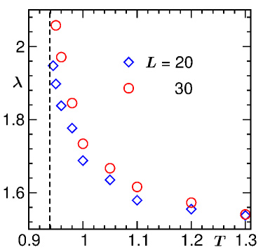
Figure 7: Plots of $\lambda$ vs $T$. Data from two different system sizes are shown. Close to the critical point the error bars are of the order of the symbol sizes. The dashed line marks the location of the critical temperature.

As stated above, at the critical point the correlation length is restricted by the system size, i.e., $\xi\sim L$ at $T=T_{c}$, so that 2DPLandau

$$\Delta X(T_{c})\sim L^{x}.$$ (18)

Far from $T_{c}$, the finite-size effects will be absent, i.e., the data will be independent of $L$. To describe the thermodynamic limit ($L\gg\xi$) and finite-size limit data by a single equation, one should introduce a bridging or FSS function $Y(y)$, to write

$$\Delta X(T)\sim Y(y)L^{x}.$$ (19)

In Eq. (19), $Y(y)$ is independent of the system size and depends upon the scaling variable $y$ ($=(L/\xi)^{1/\nu}\sim\epsilon L^{1/\nu}$), the latter being a dimensionless quantity. In the limit $y\rightarrow 0$, i.e., $T\rightarrow T_{c}$, $Y$ must be a constant so that Eq. (18) is recovered. On the other hand, in the limit $y\rightarrow\infty$ ($\xi<<L,~{}\epsilon\gg 0$), $Y$ should exhibit a power-law decay

$$Y(y)\sim y^{-x\nu},$$ (20)

so that the data are described by Eq. (17). A plot of $Y$ vs $y$, obtained by taking data from different system sizes, will exhibit data collapse, for appropriate choices of $X_{b}$, $x$ and $\nu$. Also, for the best data collapse, the large $y$ behavior of $Y$ will be consistent with Eq. (20).

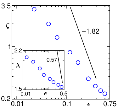
Figure 8: Plot of $\zeta$ vs $\epsilon$, on a log-log scale, for $L=30$. The solid line corresponds to the theoretical expectation. Inset shows the same exercise for $\lambda$.

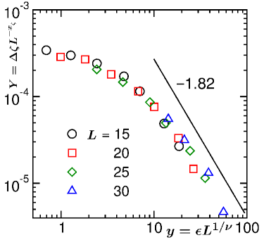
Figure 9: Finite-size scaling plot for the bulk viscosity. The scaling function $Y$ ($=\Delta\zeta L^{-x_{{}_{\zeta}}}$) is plotted vs the scaling parameter $y$ ($=\epsilon L^{1/\nu}$), on a log-log scale, using data from different system sizes. The solid line in the figure represents a power-law with the exponent being mentioned next to it.

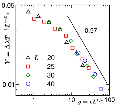
Figure 10: Finite-size scaling exercise for the thermal conductivity. Here we show $Y$ ($=\Delta\lambda T^{-1}L^{-x_{{}_{\lambda}}}$) vs $y$ ($=\epsilon L^{1/\nu}$) on a log-log scale. The solid line is a power-law, exponent of which is mentioned next to the line.

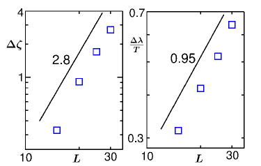
Figure 11: Log-log plots of critical parts of bulk viscosity (left) and thermal conductivity (right), vs $L$, at $T_{c}^{\rm eff}(f,L)$ with $f=1$. The solid lines are power laws. Corresponding exponent values are mentioned.

In Fig. 9, we have presented the FSS analysis result for $\zeta$, by plotting $Y(y)$ vs $y$, using data from different system sizes, mentioned on the figure. To show consistency with the theoretical predictions, in this analysis we have used $\zeta_{b}$ (background contribution for $\zeta$) as adjustable parameter and fixed $\nu$ and $x_{\zeta}$ to their theoretical values. The presented result corresponds to best collapse which is obtained for $\zeta_{b}=0.40$. Given the difficulty one encounters in calculating bulk viscosity, even a reasonably better collapse would require significant additional effort. In the limit $y\rightarrow 0$, the master curve approaches a constant value, as expected from the construction of $Y$. On the other hand, for $y\rightarrow\infty$, the master curve is showing a power-law decay with the exponent $x_{\zeta}\nu=1.82$. Similar exercise we have performed for $\lambda$, the results for which are presented in Fig. 10. Here note that, since $\Delta\lambda\sim T\epsilon^{-0.57}$, the ordinate contains the factor $T^{-1}$. In this case we have obtained best collapse for $\lambda_{{}_{b}}=1.34$.

To justify the correctness of the background values obtained above, we perform further analysis 2SRoy1 ; DKF1 ; DKF2 . This, in addition to achieving the stated objective, will provide direct information on the critical exponents as well. For this purpose, we define finite-size effective critical points as

$$T_{c}^{\rm eff}(f,L)=T_{c}+f(T_{c}^{L}-T_{c}).$$ (21)

Even though we do not have estimates of the finite-size critical points $T_{c}^{L}$, $T_{c}^{\rm eff}$ can be estimated from the fact 2MEFisher4 that $(T_{c}^{L}-T_{c})\sim L^{-1/\nu}$. Data at $T_{c}^{\rm eff}(f,L)$, for various values of $f$, will have same scaling form as that at $T_{c}^{L}$. Thus, we expect $\Delta X$ to behave as $\Delta X\sim L^{x}$, when extracted at $T_{c}^{\rm eff}(f,L)$ for a fixed value of $f$. In Fig. 11 we have performed this exercise for both $\zeta$ and $\lambda$ for $f=5$. In this process we have subtracted the values of background that we obtained above. The value of $f$ was chosen in such a way that the effective finite-size critical points do not fall in the finite-size coexistence region and corresponding values of $\epsilon$ do not exceed $0.1$. Results at various values of $T_{c}^{\rm eff}(f,L)$ were obtained by suitable interpolation using the existing temperature dependent data for different values of $L$. These results are presented on log-log scales. The data are consistent with the theoretical expectations, within about $5\%$ deviation. We could as well have estimated the backgrounds from this exercise and used the numbers in the FSS analyses of Figs. 9 and 10.

All the results on dynamics have been presented for $\rho=\rho_{c}$. As stated above, we have accumulated data over a wide range of density. Similar FSS analyses have been performed for $\rho=0.31$ and $0.32$. For these values of $\rho$, we observe that the exponent values are in reasonable agreement with the ones for $\rho=\rho_{c}$. Such small difference is consistent with the data presented in Ref. Sear1 . In this latter work, over a density range of about $5\%$ on either side of $\rho_{c}$, the thermal conductivity data showed quite flat behavior.

IV Summary

We have studied the phase behavior and the dynamic critical phenomena for vapor-liquid transition in a single component Lennard-Jones fluid in space dimension $d=3$. The phase behavior was obtained via Monte Carlo simulations 2AZPanagiotopoulos . To study the dynamic critical phenomena, we performed molecular dynamics simulations 2MPAllen ; 2DFrankel ; 2DCRapaport in microcanonical ensemble. The Green-Kubo relations 2JPHansen were used to calculate the transport quantities, viz., the bulk viscosity and the thermal conductivity. We observe strong finite-size effects, similar to the case of liquid-liquid transitions 2SKDas1 ; 2SRoy1 . Our finite-size scaling analyses, however, show that the simulation data are consistent with the theoretically predicted critical divergences. In fact, to the best of our knowledge, this is the first time the critical exponents for bulk viscosity and thermal conductivity have been quantified for a vapor-liquid transition.

Our results, along with the ones for the binary fluid 2SKDas1 ; 2SRoy1 , are compatible with the expectation that the dynamic critical phenomena of the vapor-liquid and liquid-liquid transitions belong to the same universality class, defined by model H 2PCHohenberg . Here note that the theoretical numbers for $x_{{}_{\zeta}}$ for vapor-liquid and liquid-liquid transitions are slightly different 2JKBhattacharjee1 ; 2JKBhattacharjee2 . This difference is within the error bars of computation via molecular dynamics.

Despite the similar critical exponents in vapor-liquid and liquid-liquid transitions, we have observed some differences between the two cases. Our observation of the critical range in this work is less wide compared to that of the liquid-liquid transition 2SKDas1 ; 2SRoy1 . We also have observed that the background contribution for the bulk viscosity is nonzero (though small), whereas in the liquid-liquid transition it was not needed in the analysis 2SRoy1 . Similarly, for thermal conductivity the background term plays very important role. These differences may have some connection with the symmetry of the model in the liquid-liquid case, but further investigations will be needed to confirm it.

Acknowledgment: SKD and JM acknowledge financial supports from the Department of Science and Technology, Government of India, and Marie Curie Actions plan of the European Union (FP7-PEOPLE-2013-IRSES Grant No. 612707, DIONICOS). JM is grateful to the University Grants Commission, India, for research fellowship. The $NPT$ simulation code was written with the objective of obtaining vapor-liquid coexistence curve in binary mixtures, in collaboration with J. Horbach (JH). We thank JH for important inputs with respect to this.
* das@jncasr.ac.in

References

- (1) M.E. Fisher, Rep. Prog. Phys. 30, 615 (1967).
- (2) H.E. Stanley, Introduction to Phase Transitions and Critical Phenomena (Oxford University Press, Oxford, 1971).
- (3) M.E. Fisher, Rev. Mod. Phys. 46, 597 (1974).
- (4) V. Privman, P.C. Hohenberg, and A. Aharony, in Phase Transitions and Critical Phenomena, edited by C. Domb and J.L. Lebowitz (Academic Press, New York, 1991), Vol. 14, Chap. I.
- (5) M.E. Fisher, Rev. Mod. Phys. 70, 653 (1998).
- (6) J. Zinn-Justin, Phys. Rep. 344, 159 (2001).
- (7) D.P. Landau and K. Binder, A Guide to Monte Carlo Simulations in Statistical Physics (Cambridge University Press, Cambridge, 2009).
- (8) P.C. Hohenberg and B.I. Halperin, Rev. Mod. Phys. 49, 435 (1977).
- (9) A. Onuki, Phase Transition Dynamics (Cambridge University Press, Cambridge, England, 2002).
- (10) J.V. Sengers and R.A. Perkins, “Fluids near critical points”, in Transport Properties of Fluids: Advances in Transport Properties, edited by M.J. Assael, A.R.H. Goodwin, V. Vesovic, and W.A. Wakeham (IUPAC, RSC Publishing, Cambridge, 2014), pp. 337-361.
- (11) M.A. Anisimov and J.V. Sengers, in Equations of State for Fluids and Fluid Mixtures, edited by J.V. Sengers, R.F. Kayser, C.J. Peters, and H.J. White, Jr., (Elsevier, Amsterdam, 2000), p. 381.
- (12) L. Mistura, J. Chem. Phys. 62, 4571 (1975).
- (13) H.C. Burstyn and J.V. Sengers, Phys. Rev. Lett. 45, 259 (1980).
- (14) R.A. Ferrell and J.K. Bhattacharjee, Phys. Lett. A 88, 77 (1982).
- (15) H.C. Burstyn and J.V. Sengers, Phys. Rev. A 25, 448 (1982).
- (16) R.A. Ferrell and J.K. Bhattacharjee, Phys. Rev. A 31, 1788 (1985).
- (17) G.A. Olchowy and J.V. Sengers, Phys. Rev. Lett. 61, 15 (1988).
- (18) R. Folk and G. Moser, Phys. Rev. Lett. 75, 2706 (1995).
- (19) J. Luettmer-Strathmann, J.V. Sengers, and G.A. Olchowy, J. Chem. Phys. 103, 7482 (1995).
- (20) A. Onuki, Phys. Rev. E 55, 403 (1997).
- (21) R. Folk and G. Moser, Phys. Rev. E 58, 6246 (1998).
- (22) H. Hao, R.A. Ferrell, and J.K. Bhattacharjee, Phys. Rev. E. 71, 021201 (2005).
- (23) J.K. Bhattacharjee, I. Iwanowski, and U. Kaatze, J. Chem. Phys. 131, 174502 (2009).
- (24) J.K. Bhattacharjee, U. Kaatze, and S.Z. Mirzaev, Rep. Prog. Phys. 73, 066601 (2010).
- (25) K. Jagannathan and A. Yethiraj, Phys. Rev. Lett. 93, 015701 (2004).
- (26) K. Meier, A. Laesecke, and S. Kabelac, J. Chem. Phys. 122, 014513 (2005).
- (27) K. Jagannathan and A. Yethiraj, J. Chem. Phys. 122, 244506 (2005).
- (28) A. Chen, E.H. Chimowitz, S. De, and Y. Shapir, Phys. Rev. Lett. 95, 255701 (2005).
- (29) S.K. Das, M.E. Fisher, J.V. Sengers, J. Horbach, and K. Binder, Phys. Rev. Lett. 97, 025702 (2006).
- (30) S.K. Das, J. Horbach, K. Binder, M.E. Fisher, and J.V. Sengers, J. Chem. Phys. 125, 024506 (2006).
- (31) K. Dyer, B.M. Pettitt, and G. Stell, J. Chem. Phys. 126, 034501 (2007).
- (32) S. Roy and S.K. Das, Europhys. Lett. 94, 36001 (2011).
- (33) M. Gross and F. Varnick, Phys. Rev. E 85, 056707 (2012).
- (34) S. Roy and S.K. Das, J. Chem. Phys. 139, 064505 (2013).
- (35) S. Roy and S.K. Das, J. Chem. Phys. 141, 234502 (2014).
- (36) S. Roy and S.K. Das, Eur. Phys. J. E 38, 132 (2015).
- (37) S. Roy, S. Dietrich, and F. Höfling, J. Chem. Phys. 145, 134505 (2016).
- (38) J.W. Mutoru, W. Smith, C.S. O’Hern, and A. Firozabadi, J.Chem. Phys. 138, 024317 (2013).
- (39) A.J. Bray, Adv. Phys. 51, 481 (2002).
- (40) H. Furukawa, Phys. Rev. E 36, 2288 (1987).
- (41) J.-P. Hansen and I.R. McDonald, Theory of Simple Liquids (Academic Press, London, 2008).
- (42) D.J. Searles, D.J. Evans, H.J.M. Hanley and S. Murad, Molecular Simulation 20, 385 (1998).
- (43) M.E. Fisher, in Critical Phenomena, edited by M.S. Green (Academic Press, London) 1971, p. 1.
- (44) A.Z. Panagiotopoulos, Molec. Phys. 61, 813 (1987).
- (45) P. Virnau and M. Müller, J. Chem. Phys. 120, 10925 (2004).
- (46) N.B. Wilding and K. Binder, Physica A 231, 439 (1996).
- (47) A.Z. Panagiotopoulos, J. Phys.: Condens. Matter 12, R25 (2000).
- (48) N.B. Wilding, J. Phys.: Condens. Matter 9, 585 (1997).
- (49) Y.C. Kim, E. Luijten and M.E. Fisher, Phys. Rev. Lett. 91, 065701 (2003).
- (50) C.A. Cerdeiriña, G. Orkoulas and M.E. Fisher, Phys. Rev. Lett. 116, 040601 (2016).
- (51) M.P. Allen and D.J. Tildsely, Computer Simulations of Liquids (Clarendon, Oxford, 1987).
- (52) D. Frankel and B. Smit, Understanding Molecular Simulations: From Algorithms to Applications (Academic Press, San Diego, 2002).
- (53) https://www.nist.gov/mml/csd/ chemical-informatics-research-group/ sat-tmmc-liquid-vaor-coexistence-properties-linear-2.
- (54) D.C. Rapaport, The Art of Molecular Dynamics Simulations (Cambridge University Press, Cambridge, England, 2004).
- (55) J.R. Errington and P.G. Debenedetti, J. Chem. Phys. 118, 2256 (2003).
- (56) A. Trokhymchuk and J. Alejandre, J. Chem. Phys. 111, 8510 (1999).
- (57) H.C. Burstyn, J.V. Sengers, J.K. Bhattacharjee, and R.A. Ferrell, Phys. Rev. A 28, 1567 (1983).
- (58) S.K. Das, Y.C. Kim, M.E. Fisher, Phys. Rev. Lett. 107, 215701 (2011).
- (59) S.K. Das, Y.C. Kim, M.E. Fisher, J. Chem. Phys. 137, 074902 (2012).