Dispersive Jaynes-Cummings Hamiltonian describing a two-level atom interacting with a two-level single mode field

Abstract

We investigate the time evolution of statistical properties of a single mode radiation field after its interaction with a two-level atom. The entire system is described by a dispersive Jaynes-Cummings Hamiltonian assuming the atomic state evolving from an initial superposition of its excited and ground states, $|e\rangle+|g\rangle,$ and the field evolving from an initial superposition of two excited levels, $|n_{1}\rangle+|n_{2}\rangle$. It is found that the field evolution is periodic, the period depending on the ratio $n_{2}/n_{1}.$ The energy excitation oscillates between these two states and the statististics can be either sub- or super-Poissonian, depending on the values $n_{1},$ $n_{2}$.

I Introduction

More than 50 years ago a very simple model Hamiltonian was proposed by E.T. Jaynes and F.W. Cummings (JC) to study the interaction between a two-level atom and a quantized single mode field Jaynes . The aim of the authors was to compare the quantum theory with the semi-classical one for the radiation field. Initially, no difference was observed, either using a classical field $E(t)=E_{0}cos(\omega t)$ or a quantized field assumed in one of the most nonclassical state, as the number state $|n\rangle$. Next, 17 years later a new calculation by Eberly et al in 1980 Eberly was implemented assuming the field initially in a coherent state; they showed the atom exhibiting a new nonclassical effect, then named as “collapse and revival” of the atomic inversion. The effect was observed experimentally in 1987 by G. Rempe et. al Rempe .

The JC model is written in the form ($\hbar=1$),

$$\mathcal{\hat{H}}=\omega\hat{a}^{\dagger}\hat{a}+\frac{1}{2}\omega_{0}\hat{\sigma}_{z}+\lambda(\hat{\sigma}_{+}\hat{a}+\hat{a}^{\dagger}\hat{\sigma}_{-}).$$ (1)

In the Eq.(1) $\hat{a}$ ($\hat{a}^{{\dagger}}$) stands for the annihilation (creation) operator, $\sigma_{-}$ ($\sigma_{+}$) is the lowering (raising) operator, $\hat{n}=\hat{a}^{{\dagger}}\hat{a}$ is the number operator, $\omega$ $(\omega_{0})$ is the field (atomic) frequency, and $\lambda$ stands for the atom-field coupling. One identifies $\mathcal{\hat{H}}_{0}=\omega\hat{a}^{\dagger}\hat{a}+\frac{1}{2}\omega_{0}\hat{\sigma}_{z}$ as the “free Hamiltonian” whereas $\hat{V}=$ $\lambda(\hat{\sigma}_{+}\hat{a}+\hat{a}^{\dagger}\hat{\sigma}_{-})$ is the “interaction Hamiltonian”. When $\omega=$ $\omega_{0}$ the atom and the radiation field are resonant and we have $[\mathcal{\hat{H}}_{0},\hat{V}]=0$; as consequence the interaction $\hat{V}$ in the interaction picture is the same, namely, $\hat{V}^{I}=\hat{V}$, and this makes easier the subsequent calculations. Now, when $\Delta\omega=\omega_{0}-\omega\neq 0$ the atom and the field are no longer in resonance; in this case two alternatives may occur: they can be either near the resonance, which means $\frac{\Delta\omega}{\lambda}\approx 1,$ or far from resonance, $\frac{\Delta\omega}{\lambda}\gg 1$. In the first case we sum and subtract $(\omega\hat{\sigma}_{z}/2)$ to the resonant case and obtain,

$$\mathcal{\hat{H}}^{\prime}=\omega(\hat{a}^{\dagger}\hat{a}+\frac{1}{2}\hat{\sigma}_{z})+\frac{1}{2}\Delta\omega\hat{\sigma}_{z}+\lambda(\hat{\sigma}_{+}\hat{a}+\hat{a}^{\dagger}\hat{\sigma}_{-}).$$ (2)

In Eq.(2), the following changes took place:
the new “free Hamiltonian” is $\mathcal{\hat{H}}_{0}^{\prime}=\omega(\hat{a}^{\dagger}\hat{a}+\frac{1}{2}\hat{\sigma}_{z})$ whereas $\hat{V}^{\prime}=\frac{1}{2}\Delta\omega\hat{\sigma}_{z}+\lambda(\hat{\sigma}_{+}\hat{a}+\hat{\sigma}_{-}\hat{a}^{{\dagger}})$ stands for the new and effective interaction. Then, while $[\mathcal{\hat{H}}_{0},\hat{V}]\neq 0$ we have that $[\mathcal{\hat{H}}_{0}^{\prime},\hat{V}^{\prime}]=0$ and, as consequence, the subsequent calculations become easier again, since $\hat{V}^{\prime I}=\hat{V}^{\prime}$. In both previous cases (in-resonance and off-resonance) we get exact solutions.

Now, when the detuning $\Delta\omega$ is large, namely: $\frac{\Delta\omega}{\lambda}\gg 1$, the mentioned easiness to solve the problem no longer occurs. In this case a good approximation can be obtained from an equivalent interaction Hamiltonian $\hat{V}^{\prime\prime}$, constructed from the Eq.(2), named dispersive JC model, given by

$$\hat{V}^{\prime\prime}=\lambda^{\prime}\hat{n}(|i\rangle\langle i|+|e\rangle\langle e|),$$ (3)

where $\lambda^{\prime}$ is the effective coupling involving the parameter $\lambda$ and the frequency shift $\Delta\omega$ of the cavity (detuning $\Delta\omega\gg\lambda$).

II Dispersive JC Model

The Eq.(3) represents the dispersive JC model: it describes the field interacting with a 2-level atom, with respect to the levels $|e\rangle$ and $|i\rangle$, where $|i\rangle$ represents a virtual state. Hence, when initially an atom previously prepared in a superposed state $|\psi_{A}\rangle=(|e\rangle+|g\rangle)/\sqrt{2}$ Nota enters a microwave cavity that contains a field in an arbitrary normalized state $|\psi_{F}\rangle,$ there is no exchange of energy between the atom and the field with respect to the atomic levels $|e\rangle$ and $|g\rangle$.

In this scenario, the unitary operator $\hat{U}(t)=\exp(-it\hat{V}^{\prime\prime})=\exp[-it\lambda^{\prime}\hat{n}(|i\rangle\langle i|+|e\rangle\langle e|)]$ describes in which way the atom-field system evolves in time. Thus we have,

$$|\psi_{AF}(t)\rangle=\frac{1}{\sqrt{2}}\hat{U}(t)[(|e\rangle+|g\rangle)|\psi_{F}\rangle].$$ (4)

Next, after using some algebra involving the equality $(\hat{V}^{\prime\prime})^{n}=\omega^{n}\hat{n}^{n}(|i\rangle\langle i|+(-1)^{n}|e\rangle\langle e|)$ we obtain the entangled state, with $\phi(t)=\lambda^{\prime}t,$

$$|\psi_{AF}(t)\rangle=|g\rangle|\psi_{F}\rangle+|e\rangle(e^{i\phi(t)\hat{n}}|\psi_{F}\rangle).$$ (5)

The Eq.(5) shows that the dispersive interaction affects only the phase of the field, thus no exchange of energy occurs between the atom and the field. Also, the Eq.(5) corresponds to the state of the combined atom-field system right after the atom has crossed the cavity, at an intant of time $t=\tau$. The evolution of the field state occurs during the atom-field interaction in the time interval $0\leq t\leq\tau$; $\tau$ is defined by the speed of the atom and the length of the cavity.

The JC model in these three versions: resonant, near resonance, and far from resonance, has been explored by many researchers. As examples of works in the first scenario we mention the Refs. Simon ; Meystre ; in the second scenario Scully ; Knight and in the third Bertet ; Peixoto . In the latter case, the approach became important to treat the Schrödinger cat problem Haroche1 ; Kuklinski . It is worth mentioning that the JC model may include various extensions: one of them adds the counter rotating term $\lambda^{\prime}(\hat{a}^{\dagger}\hat{\sigma}_{+}+\hat{a}\hat{\sigma}_{-})$ to the usual interaction Walls ; it comes from the original interaction, $\hat{V}=\mathbf{\hat{d}}\cdot\mathbf{\hat{E},}$ where $\mathbf{\hat{d}\sim(}\hat{\sigma}_{+}+\hat{\sigma}_{-})$ and $\mathbf{\hat{E}\sim(}\hat{a}^{\dagger}+\hat{a})$; another extension treats the case of multiphoton interaction $\lambda[\hat{a}^{p}\hat{\sigma}_{+}+(\hat{a}^{\dagger})^{p}\hat{\sigma}_{-}],$ $p=2,3,4,...$ Singh ; Chaba ; Gerry ; etc. Other kinds of extensions also appear in the literature: one of them extends the JC model to another, named Buck-Sukumar model Buck ; another interpolates between the JC model to the Sivakumar model Siva ; yet another going from the JC model to the Rodríguez–Lara model Lara ; a model that includes ‘quonic’ particles was also proposed: it extends the JC Model to the Shanta-Chaturvedi-Arinivasan model Shanta . A generalized model (VB model) that includes all these previous (bosonic) models has been proposed Valverde . Although not very usual, the JC model is also treated in the Heisenberg picture Stenholm . Now, according to the Eq.(5),if we let the traveling atom traverse a second Ramsey zone Haroche2 , this apparatus leads the atom in the state $|e\rangle$ to the superposed state $(|e\rangle+|g\rangle)$ and leads the atom in the state $|g\rangle$ to $(|g\rangle-|e\rangle)$. Then we get,

$$|\psi_{AF}(t)\rangle=|g\rangle(|\psi_{F}\rangle+|\psi_{F}^{\prime}\rangle)+|e\rangle(|\psi_{F}^{\prime}\rangle-|\psi_{F}\rangle),$$ (6)

where $|\psi_{F}^{\prime}\rangle=e^{i\phi\hat{n}}|\psi_{F}\rangle$. Next, if the atom is detected in its ground state $|g\rangle$, the field inside cavity is projected in the even superposition $|\psi_{F}(t)\rangle=|\psi_{F}\rangle+e^{i\phi\hat{n}}|\psi_{F}\rangle$. As an application we assume the field state initially in the normalized superposition of two excited number state malboui : $|\psi_{F}(0)\rangle=(|n_{1}\rangle+|n_{2}\rangle)/\sqrt{2}$. Substituting this state in the Eq.(6) we obtain the evolved field in the state, with $\phi=\phi(t)=\lambda^{\prime}t$,

$$|\psi_{F}(t)\rangle = \frac{1}{\sqrt{2}}[(|n_{1}\rangle+|n_{2}\rangle)+(e^{i\phi\hat{n}_{1}}|n_{1}\rangle+e^{i\phi\hat{n}_{2}}|n_{2}\rangle)]$$

$$= \frac{2}{\sqrt{2}}[e^{\frac{i\phi n_{1}}{2}}(\cos\frac{\phi n_{1}}{2})|n_{1}\rangle+e^{\frac{i\phi n_{2}}{2}}(\cos\frac{\phi n_{2}}{2})|n_{2}\rangle].$$

We now can write the normalized state as

$$|\psi_{F}(t)\rangle=\eta[e^{\frac{i\phi n_{1}}{2}}(\cos\frac{\phi n_{1}}{2})|n_{1}\rangle+e^{\frac{i\phi n_{2}}{2}}(\cos\frac{\phi n_{2}}{2})|n_{2}\rangle],$$ (8)

where $\eta=(\cos^{2}\theta_{1}+\cos^{2}\theta_{2})^{-1/2}$ is the normalization factor, with $\theta_{i}=\phi n_{i}/2,$ $i=1,2.$

III Statistical Properties

The result in Eq.(8) allows us to obtain statistical properties of the field, as follows:

III.1 Statistical Distribution

From the Eq.(8) we obtain the time evolution of the statistical distribution $P_{n}(t)$. We have,

$$P_{n}(t) = |\langle n|\psi_{F}(t)\rangle|^{2}$$

$$= \eta^{2}|e^{\frac{i\phi n_{1}}{2}}(\cos\frac{\phi n_{1}}{2})\delta_{n,n_{1}}+e^{\frac{i\phi n_{2}}{2}}(\cos\frac{\phi n_{2}}{2})\delta_{n,n_{2}}|^{2}.$$

Since in this case we find that $P_{n}(t)=1$ for all times, then the relevant behavior concerns the statistics $P_{n_{1}}(t)$ and $P_{n_{2}}(t):$ they show in which way the exchange of excitations occurs between the components $|n_{1}\rangle$ and $|n_{2}\rangle$. Figs.1(a), 1(b), 1(c) and 1(d) show the time evolution of the statistical distributions $P_{n_{1}}(t)$ and $P_{n_{2}}(t)$ for the field in the state $|\psi_{F}(t)\rangle$, for various values of the excitations $n_{1}$ and $n_{2}$. The behaviors of these distributions are oscillatory, e.g., with period $\tau=2\pi$ for the pairs ($n_{1}=1$, $n_{2}=3$) and ($n_{1}=1$, $n_{2}=2$) and $\tau=\pi$ for the pair ($n_{1}=2$, $n_{2}=6$) and $\tau=2\pi/5$ for the pair ($n_{1}=5$, $n_{2}=10$). We note that, although having different periods, all pairs $(n_{1},n_{2})$ and $(n_{1}^{\prime},\,n_{2}^{\prime})$ have the same behavior when $n_{1}^{\prime}/n_{1}=n_{2}^{\prime}/n_{2}=p$, with $p=2,\,3,\,4,...\,$In addition we observe that when $P(n_{i})=1$ all field excitation concentrates into the component $|n_{i}\rangle$, as it should. For example, the state $|n_{1}\rangle=|1\rangle$ becomes pure at $\tau^{\prime}=1.05$ and $\tau^{\prime\prime}=5.24$ (in Fig.1(a)) and at $\tau^{\prime}=\pi/2$ and $\tau^{\prime\prime}=3\pi/2$ (in Fig.1(c)). At these points the entire field state becomes a number state, $|\psi_{F}(t)\rangle=|n_{1}\rangle.$

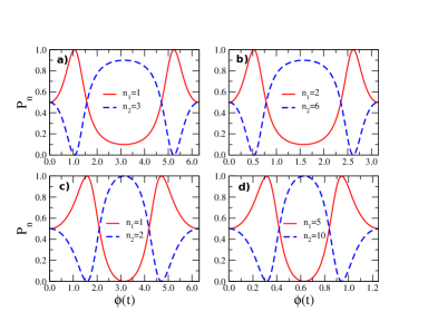
Figure 1: Time evolution of statistical distribution for the two field components $|n_{1}\rangle$ and $|n_{2}\rangle$, it shows in which way these components exchange their energies: (a) for $n_{1}=1$ and $n_{2}=3$; (b) for $n_{1}=2$ and $n_{2}=6$; (c) for $n_{1}=1$ and $n_{2}=2$; (d) for $n_{1}=5$ and $n_{2}=10$.

III.2 Mandel Parameter

The Mandel parameter informs whether the statistics is either Poissonian, sub-Poissonian or super-Poissonian Mandel . To this end we must first calculate the variance of photon number, $\langle(\triangle\hat{n})^{2}\rangle=\langle\hat{n}^{2}\rangle-\langle\hat{n}\rangle^{2}.$ From the Eq.(8) we obtain, for $\langle\hat{n}(\phi)\rangle$, $\langle\hat{n}^{2}(\phi)\rangle$ and $\langle\hat{n}(\phi)\rangle^{2}$, with $\phi=\phi(t)=\lambda^{\prime}t$,

$$\langle\hat{n}(\phi)\rangle=\eta^{2}[n_{1}\cos^{2}(\frac{\phi n_{1}}{2})+n_{2}\cos^{2}(\frac{\phi n_{2}}{2})],$$ (10)

$$\langle\hat{n}^{2}(\phi)\rangle=\eta^{2}[n_{1}^{2}\cos^{2}(\frac{\phi n_{1}}{2})+n_{2}^{2}\cos^{2}(\frac{\phi n_{2}}{2})],$$ (11)

and $\langle\hat{n}(\phi)\rangle^{2}$ is obtained from the Eq.(10). Thus, from Eqs.(10) and (11) we obtain the Mandel parameter.

$$Q = \frac{\langle(\Delta\hat{n})^{2}\rangle-\langle\hat{n}\rangle}{\langle\hat{n}\rangle}$$ (12)

$$= \frac{1}{\langle\hat{n}\rangle}\{\eta^{2}[n_{1}^{2}\cos^{2}(\frac{\phi n_{1}}{2})+n_{2}^{2}\cos^{2}(\frac{\phi n_{2}}{2})]$$

$$-\eta^{4}[n_{1}^{2}\cos^{4}(\frac{\phi n_{1}}{2})+n_{2}^{2}\cos^{4}(\frac{\phi n_{2}}{2})$$

$$+2n_{1}n_{2}\cos^{2}(\frac{\phi n_{1}}{2})\cos^{2}(\frac{\phi n_{2}}{2})]-\langle\hat{n}\rangle\}.$$

Figs.2(a), 2(b) and 2(c) show the evolution of the Mandel parameter for various excitation values of the initial excitations in the components $|n_{1}\rangle$ and $|n_{2}\rangle$.

Figure 2: (a)-Plots for the Mandel parameters for the pairs $(n_{1},n_{2})=(4,5)$ and $(8,10)$ respectively; (b)- Same as in Fig.2(a), for $(n_{1},n_{2})=(1,3)$ and $(3,9)$; (c) Same as in Fig.2(a), for $(n_{1},n_{2})=(1,5)$ and $(2,10)$.

All plots in Fig.2(a) exhibit the sub-Poissonian effect ($-1<Q<0$) during their respective periods $\tau=2\pi$ and $\tau=\pi$ for the pairs $(n_{1},n_{2})$: $(4,5)$ and $(8,10)$, respectively. In Fig.2(b) the pair $(1,3)$ exhibit sub-Poissonian effect during all period, however, the pair ($3,9$) exhibit sub- and super-Poissonian effect during the period $\tau=2\pi/3$. The sub-Poissonian effect is shown for very short time intervals in Fig.2(c); Concerning the Fig.2(c), the state remains sub-Poissonian for times in the respective periods, as also shown in Fig.2(b).

Now, all results obtained above can be extended to initial field states with two Fock components having unequal weights, e.g., $|\psi_{F}(0)\rangle=c_{1}|n_{1}\rangle+c_{2}|n_{2}\rangle$ with $|c_{1}|^{2}+$ $|c_{2}|^{2}=1$. At this point a few words should be devoted on how to get an available initial superposed state of the type used here, as $|\psi_{F}(0)\rangle=(|n_{1}\rangle+|n_{2}\rangle)/\sqrt{2}$ or one of its extensions. In Fig.(3) below, the Fig.3(a) represents a coherent state $|\alpha\rangle$ inside a good cavity. As well known, by making a conveniently prepared two-level atom that crosses the cavity and interacts with a coherent state, it transforms the coherent state into a superposition of two coherent states, including the so called “Schrodinger-cat” state when a rotation by an angle $\theta=\pi$ in the phase space affects the coherent state Haroche1 .

Figure 3: Photon number distribition displaying the creation of the superposition of two number states. a) $\alpha=3.0$ and $N=2;$ b) $\alpha=1.009$ and $N=2;$ c) $\alpha=3.482$ and $N=3;$ d) $\alpha=4.899$ and $N=4.$

Now, as one example, the Ref.malboui studied the generation of various superposition states when $N$ atoms cross the cavity, $N=1,2,3,...$ suscessively with convenient speeds $\upsilon_{N}=\upsilon_{N-1}/2.$ The wavefunction describing the system is given by,

$$\left|\Psi_{N}^{\pm}(\alpha)\right\rangle=\sum\limits_{n=0}^{\infty}C_{N}^{\pm}(n;\alpha)\left|n\right\rangle,$$ (13)

where,

$$C_{N}^{\pm}(n;\alpha) = \left\langle n|\Psi_{N}^{\pm}(\alpha)\right\rangle,$$ (14)

$$= [2^{2N}\exp(\alpha^{2})\beta_{N}^{\pm}(\alpha^{2})]^{-1/2}\exp(-\left|\alpha\right|^{2}/2)\alpha^{n}$$

$$\times\frac{(-1)^{n}\pm 1}{\sqrt{n!}}\sum\limits_{j=0}^{2^{N-1}-1}\exp(\frac{in\pi j}{2^{N-1}}),$$

with $\beta_{N}^{\pm}(\alpha^{2})$ for $N>1,$ standing for,

$$\beta_{N}^{\pm}(\alpha^{2}) = \frac{1}{2^{N-1}}\beta_{1}^{\pm}(\alpha^{2})+\frac{1}{2^{2(N-1)}}\sum\limits_{k=0}^{2^{N-1}-1}\{(2^{N}-2k)$$

$$\times\cos[\alpha^{2}\sin(\pi k/2^{N-1})]\beta_{1}^{\pm}[\alpha^{2}\cos(\pi k/2^{N-1})]\},$$

and $\beta_{1}^{\pm}(\alpha^{2})=\frac{1}{2}[\exp(\alpha^{2})\pm\exp(-\alpha^{2})]$  for $N=1$. Thus the probability of photon number distribution is obtained from the expression,

$$P_{N}^{\pm}(n;\alpha)=\left|\left\langle n|\Psi_{N}^{\pm}(\alpha)\right\rangle\right|^{2},$$ (16)

the sign $(+)$ standing for the even state and sign $(-)$ for the odd state.

From convenient choices of values of $\alpha$ and $N$ one gets the results displayed in Fig.3(b), 3(c), and 3(d). Fig.3(b) is one of the results when passing two atoms, for the states $|1\rangle$ and $|3\rangle$; Fig.3(c) concerns the case of three atoms, leading to the states $|8\rangle$ and $|16\rangle$; Fig.3(d) is the case of four atoms leading to the states $|16\rangle$ and $|32\rangle$. Other pairs of Fock components can also be obtained, as the approximate pair $|4\rangle$ and $|8\rangle$ shown in Fig.4(a) of Ref.malboui , using two atoms.

IV Conclusion

The plots of the statistical distributions $P_{n_{1}}$ and $P_{n_{2}}$ show in which way the field state $|\psi_{F}(t)\rangle$ shares its excitation to components $|n_{1}\rangle$ and $|n_{2}\rangle$. We note the similarities that occur for the pairs of components $|n_{1}\rangle,$ $|n_{2}\rangle$ and $|n_{1}^{\prime}\rangle,$ $|n_{2}^{\prime}\rangle$ when $n_{1}^{\prime}/n_{1}=n_{2}^{\prime}/n=p,$ $p=1,2,3,...$; they show the same behavior, but in different periods, e.g., one of them being $\tau$ the other is $\tau^{\prime}=\tau/p.$ The plots of the Mandel parameter show the occurrence of sub-Poissonian statistics in Fig.2(a) and (partial) super-Poissonian statistics in Fig.2(b) and 2(c). Moreover, we verify that the larger the difference between the values $n_{1}$ and $n_{2}$ $(n_{2}-n_{1}\gg 1)$, the larger is the super-Poissonian character of the statistics. Again, the same similarities found in Fig.1 is also observed in Fig.2 for the case $n_{1}^{\prime}/n_{1}=n_{2}^{\prime}/n=p$. During all the state evolution no squeezing effect was observed and, according to the Ref.Mandel , one would observe this effect only when the field state $|\psi_{F}(t)\rangle$ can distribute his excitation to more than two Fock components. Finally, some words were dedicated on how to prepare a generalized initial state $|\psi_{F}(0)\rangle=c_{1}|n_{1}\rangle+c_{2}|n_{2}\rangle,$ as one of them assumed in this report.

V Acknowledgements

We thank the Brazilian funding agencies CAPES, CNPq and FAPEG for partial supports.

References

- (1) E.T. Jaynes, F.W. Cummings, Comparison of quantum and semiclassical radiation theories with application to the beam maser, Proc. IEEE, 51, 89 (1963).
- (2) J.H. Eberly, N.B. Narozhny, J.J. Sanchez-Mondragon, Periodic spontaneous collapse and revival in a simple quantum model, Phys. Rev. Lett. 44, 1323 (1980).
- (3) G. Rempe, H. Walther, and N. Klein, Observation of quantum collapse and revival in one atom maser, Phys. Rev. Lett. 58, 353 (1987).
- (4) This superposed state is obtained by making the atom in its excited state crossing a Ramsey zone.
- (5) Simon J. D. Phoenix, P. L. Knight, Establishment of an entangled atom-field state in the Jaynes-Cummings model, Phys. Rev. A 44, 6023 (1991).
- (6) P. Meystre, M.S. Zubairy, Squeezed states in the Jaynes-Cummings model, Phys. Lett. A, 89, 390 (1982).
- (7) Shi-Yao Zhu, Marlan O. Scully, Evolution of squeezed states in the Jaynes-Cummings model, Phys. Lett. A 130, 101 (1988).
- (8) P.L. Knight and P.M. Radmore, Quantum Revival of a two-level system driven by chaotic radiation, 90A, Phys. Lett. 90A, 26, 342 (1982).
- (9) P. Bertet, A. Auffeves, P. Maioli, S. Osnaghi, T. Meunier, M. Brune, J. M. Raimond, and S. Haroche, Direct Measurement of the Wigner Function of a One-Photon Fock State in a Cavity, Phys. Rev. Lett. 89, 200402 (2002).
- (10) J. G. Peixoto de Faria and M. C. Nemes, Dissipative dynamics of the Jaynes-Cummings model in the dispersive approximation: Analytical results, Phys. Rev. A 59, 3918 (1999).
- (11) S. Haroche, Nobel Lecture: Controlling photons in a box and exploring the quantum to classical boundary, Rev. Mod. Phys. 85, 1083 (2013).
- (12) J. R. Kuklinski and J. L. Madajczy, Strong sneezing in the Jaynes-Cimmings model, Phys. Rev. A, 37, 3175 (1988).
- (13) D. F. Walls, G. J. Milburn, Quantum Optics, Springer-Verlag, NY (1994), p.16.
- (14) Surendra Singh, Field statistics in some generalized Jaynes-Cummings models, Phys. Rev. A 25, 3206 (1982).
- (15) Chaba, A.; Baseia, B.; Wang, C. ; Vyas, R. ; Baseia, Multiphoton interaction of a phased atom with a single mode field, Physica A, 232, 273 (1996).
- (16) Cristopher C. Gerry, Two photon Jaynes Cummings model interactiong with the squeezed vacuum, Phys. Rev. A 37, 2683 (1988).
- (17) B. Buck, C. V. Sukumar; Exactly soluble model of atom-phonon coupling showing periodic decay and revival, Phys. Lett. A, 81, 132 (1981).
- (18) S. Sivakumar, Interpolating coherent states for Heisenberg–Weyl and single-photon SU(1,1) algebras, J. Phys. A: Math. Gen. 35, 6755–6766 (2002).
- (19) B. M. Rodríguez–Lara, Intensity-dependent quantum Rabi model: spectrum, supersymmetric partner, and optical simulation, J. Opt. Soc. Am. B 31, 1719 (2014).
- (20) P. Shanta, S. Chaturvedi, V. Srinivasan, A Model Which Interpolates Between the Jaynes-Cummings Model and the Buck-Sukumar Model, J. Mod. Opt., 39, 1301 (1992).
- (21) C. Valverde, B. Baseia, On the paradoxical evolution of the number of photons in a new model of interpolating Hamiltonians, arXiv:1609.01665v1 [quant-ph].
- (22) S. Stenholm, Quantum theory of electromagnetic fields interacting with atoms and molecules, Physics Reports, 6, 1-121 (1973).
- (23) M. Brune, S. Haroche, J. M. Raimond, L. Davidovich, and N. Zagury, Manipulation of photons in a cavity by dispersive atom-field coupling: Quantum-nondemolition measurements and generation of “Schrödinger cat” states, Phys. Rev. A 45, 5193 (1992).
- (24) J.M.C. Malbouisson, B. Baseia, Higher generation of Schrodinger cat states in cavity QED, J. Mod. Optics, 46, 2015 (1999), p. 2022.
- (25) Mandel, L., Sub-Poissonian photon statistics in resonance fluorescence, Opt. Lett. 4:205 (1979).