Experimental time-optimal universal control of spin qubits in solids

Abstract

Quantum control of systems plays an important role in modern science and technology. The ultimate goal of quantum control is to achieve high fidelity universal control in a time-optimal way. Although high fidelity universal control has been reported in various quantum systems, experimental implementation of time-optimal universal control remains elusive. Here we report the experimental realization of time-optimal universal control of spin qubits in diamond. By generalizing a recent method for solving quantum brachistochrone equations [X. Wang et al., Phys. Rev. Lett. 114, 170501 (2015)], we obtained accurate minimum time protocols for multiple qubits with fixed qubit interactions and a constrained control field. Single- and two-qubit time-optimal gates are experimentally implemented with fidelities of $99\%$ obtained via quantum process tomography. Our work provides a time-optimal route to achieve accurate quantum control and unlocks new capabilities for the emerging field of time-optimal control in general quantum systems.

Time-optimal control (TOC), including the famous examples of the brachistochrone problem IEEEControlSystMag_Sussmann and the Zermelo navigation problem ZAngewMathMech_Zermelo , has been widely investigated for over three centuries. TOC of quantum systems has recently attracted great interest due to the rapid development of quantum information processing and quantum metrology. Because the ever-present noise from the environment degrades quantum states or operations over time, generating the fastest possible evolution by TOC becomes a preferable choice for realizing precise quantum control in the presence of noise. To obtain accurate TOC protocols is difficult because both the fidelity and time should be optimized. Analytical methods utilizing the Pontryagin maximum principle or the geometry of the unitary group are applicable only to specific problems and constraints PRA_Glaser_2001 ; PRA_Brockett ; PRA_Yuan_2005 ; PRA_Fisher_2009 ; PRA_Boozer ; PRL_Hegerfeldt ; PRA_Garon ; PRA_Yuan_2015 . Recently, the quantum brachistochrone equation (QBE) has been proposed to provide a general framework for finding time-optimal state evolutions or unitary operations PRL_Carlini ; PRA_Carlini ; PhDThesis_Okudaira ; PRL_Rezakhani ; JPA_Carlini_2011 ; PRA_Carlini_2012 ; JPA_Carlini_2013 ; PRL_Mohseni . The QBE has been applied to some cases where analytic solutions exist JPA_Carlini_2011 ; PRA_Carlini_2012 ; JPA_Carlini_2013 . For problems where the QBE cannot be analytically solved, an effective numerical method has been developed PRL_Mohseni . The relationship between TOC and gate complexity has also been explored Science_Nielsen ; PRA_Koike . Experimental TOC has been implemented only in single-qubit systems NaturePhys_Morsch ; PRL_Sugny ; PRB_Gershoni , while experimental time-optimal universal control, which requires universal single-qubit gates as well as a non-trivial two-qubit gate, has not been reported.

Here, we demonstrate the first experimental time-optimal universal control of a two-qubit system, which consists of an electron spin and a nuclear spin of a nitrogen-vacancy (NV) center in diamond. High-fidelity single- and two-qubit gates are realized with fidelities of $99\%$ obtained via quantum process tomography. Our results show that TOC provides a novel route to achieve precise universal quantum control. The approach to realize time-optimal control of multiple qubits can be applied to other quantum systems.

As shown in Fig. 1, the quantum system is driven by the Hamiltonian $H(t)$, which is described by the Schrödinger equation $\dot{U}=-iH(t)U$, with boundary conditions $U(0)=I$ and $U(T)=U_{F}$ (we set $\hbar=1$). Different Hamiltonians $H(t)$ make the evolutions of the system follow different paths (labeled by $\Gamma_{i}$) to the same unitary operation $U_{F}$. The path with the minimal time cost can be obtained by solving the QBE PRA_Carlini together with the Schrödinger equation. The QBE is written as

$$\dot{F}=-i[H,F],$$ (1)

where $F=\partial L_{C}/\partial H$ and $L_{C}=\sum_{j}\lambda_{j}f_{j}(H)$, with $\lambda_{j}$ the Lagrange multiplier. One physically relevant constraint is the finite energy bandwidth described as $f_{0}(H)\equiv[{\rm Tr}(H^{2})-E^{2}]/2=0$, where $E$ is a constant. Reference PRL_Mohseni, provides a method to obtain the accurate minimum-time protocol by solving the QBE.

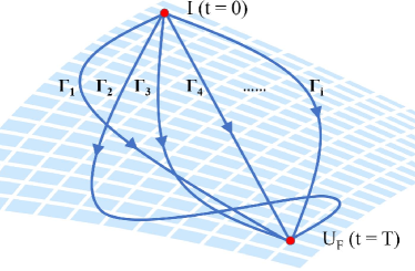
Figure 1: (color online). Schematic representation of quantum TOC. Blue lines represent paths of quantum evolution in the SU($2^{n}$) operator space, where $n$ stands for the number of qubits. To realize a target evolution operator $U_{\textrm{F}}$ at $t=T$ starting from the identity operator $I$ at $t=0$, there are several choices of evolution path $\Gamma_{i}~{}(i=1,2\ldots)$. The goal of TOC is to figure out which evolution costs the minimum time $T$.

In realistic physical systems, part of the Hamiltonian $H$ is usually time independent (e.g., fixed couplings between spin qubits), and the reasonable constraint for the energy is actually for the time variable part (e.g., the shaped microwave pulse with bounded power). These have been recently recognized and investigated as the quantum Zermelo navigation problem PRL_Meier ; PRA_Stepney . The original QBE is not able to provide a solution to this problem directly. Here, we rewrite the Hamiltonian $H(t)$ as $H=H_{0}+H_{c}(t)$, where the drift Hamiltonian $H_{0}$ stands for the time invariable part and $H_{c}(t)$ stands for the control Hamiltonian. The drift Hamiltonian $H_{0}$ can be the fixed spin couplings or nonzero constant external magnetic field. The control Hamiltonian $H_{c}(t)$ can be a controllable external magnetic field or adjustable couplings between qubits. The constraint of the finite energy bandwidth is modified to $f_{0}(H_{c})=0$. Then, the TOC of multiple qubits, which is experimentally feasible, can be obtained by solving the QBE with the mentioned improvements (see Section II in Supplementary Material). This method can be taken as the generalization of the method in Ref. PRL_Mohseni, , which is the case of $H_{0}=0$.

We experimentally demonstrate TOC of single- and two-qubit on an NV center in diamond. The NV center is composed of an electron spin and a nitrogen nuclear spin. A static magnetic field of about 500 G is applied along the NV symmetry axis ([1 1 1] crystal axis) and removes the degeneracy between the $|m_{S}=+1\rangle$ and $|m_{S}=-1\rangle$ electron spin states. Under such a magnetic field, the spin state of the NV center is effectively polarized to $|m_{S}=0,m_{I}=+1\rangle$ when a 532 nm laser pulse is applied PRL_Wrachtrup . Microwave pulses driving the electron spin transition $|m_{S}=0\rangle$ to $|m_{S}=-1\rangle$ and radio-frequency pulses driving the nuclear spin transition $|m_{I}=+1\rangle$ to $|m_{I}=0\rangle$ are utilized to manipulate the spin states. The $|m_{S}=+1\rangle$ electron spin level and $|m_{I}=-1\rangle$ nuclear spin level remain idle due to large detuning. TOC is demonstrated on the two-qubit system composed by $|m_{S}=0,m_{I}=+1\rangle$, $|m_{S}=-1,m_{I}=+1\rangle$, $|m_{S}=0,m_{I}=0\rangle$, and $|m_{S}=-1,m_{I}=0\rangle$ without considering the other spin levels (see Section I and Fig. S1 in Supplementary Material).

The experiment was implemented on an NV center in $[100]$ face bulk diamond. The nitrogen concentration in the diamond was less than 5 ppb and the abundance of ¹³C was at the natural level of 1.1%. The NV center was optically addressed by a home-built confocal microscope. Spin-state initialization and detection of the NV center were realized with a 532 nm green laser controlled by an acousto-optic modulator (ISOMET, power leakage ratio $\sim$1/1000). To preserve the NV center’s longitudinal relaxation time from laser leakage effects, the laser beam was passed twice through the acousto-optic modulator before going through an oil objective (Olympus, PLAPON 60*O, NA 1.42). The phonon sideband fluorescence (wavelength 650$\sim$800 nm) went through the same oil objective and was collected by an avalanche photodiode (Perkin Elmer, SPCM-AQRH-14) with a counter card. A solid immersion lens was created around the NV center to increase the fluorescence collection efficiency. The magnetic field was provided by a permanent magnet and aligned by monitoring the variation of fluorescence counts. The spin states of the NV center were manipulated with microwave and radio-frequency pulses. The microwave and radio-frequency pulses were generated by an arbitrary waveform generator (Keysight M8190A), amplified individually with power amplifiers (Mini Circuits ZHL-30W-252-S+ for microwave pulses and LZY-22+ for radio-frequency pulses), and combined with a diplexer (Marki DPX-1). An ultra-broadband coplanar waveguide with $15~{}$GHz bandwidth was designed and fabricated to feed the microwave and radio-frequency pulses.

Universal control of a single qubit requires the ability to realize rotations around two different axes of the Bloch sphere. The evolution operator is denoted with $R(\hat{\mathbf{n}},\theta)$, corresponding to a rotation of angle $\theta$ around axis $\mathbf{\hat{n}}=\mathbf{\hat{x}}\sin\gamma\cos\varphi+\mathbf{\hat{y}}\sin\gamma\sin\varphi+\mathbf{\hat{z}}\cos\gamma$. The method to realize TOC gates, which rotate the quantum states along two different axes, is detailed in Section II in Supplementary Material. We take a target unitary transformation $R(\hat{\mathbf{z}},\theta)$ on the electron spin qubit as an example. In the rotating frame, $H_{0}=2\pi\delta S_{z}$, $H_{c}(t)=2\pi\nu_{1}[\cos\phi(t)S_{x}+\sin\phi(t)S_{y}]$, where $S_{x}$, $S_{y}$, and $S_{z}$ are effective spin operators of the electron spin qubit, $\delta$ is the detuning term, $\nu_{1}>0$ stands for the amplitude of the microwave pulse, and $\phi(t)$ is the phase of microwave pulse. The control Hamiltonian $H_{c}$ satisfies two constraints, which are $f_{0}(H_{c})\equiv[{\rm Tr}(H_{c}^{2})-2\pi^{2}\nu_{1}^{2}]/2=0$ and $f_{1}(H_{c})\equiv{\rm Tr}(H_{c}S_{z})=0$. The solution to the QBE is $\phi(t)=2\pi\eta t+\phi(0)$, where $\eta$ is a constant. Then the detailed parameters of the control Hamiltonian [e.g., $\eta$ and $\phi(t)$] and the minimum evolution time $T$ can be obtained by further solving the Schrödinger equation. By following the procedure described above, we can derive the explicit analytical solutions to the TOC for realizing $R(\hat{\mathbf{z}},\theta)$. Without loss of generality, we present the analytical solution when $\delta\geq 0$ and $\theta\in[0,2\pi)$. If $\theta<\pi(1+\sqrt{3}\delta/\nu_{1})$, the minimum evolution time $T=[\delta(\theta/2\pi-1)+\sqrt{\nu_{1}^{2}+\delta^{2}-\nu_{1}^{2}(\theta/2\pi-1)^{2}}]/(\nu_{1}^{2}+\delta^{2})$; otherwise, the minimum evolution time becomes $T=[\delta\theta/2\pi+\sqrt{\nu_{1}^{2}+\delta^{2}-\nu_{1}^{2}(\theta/2\pi)^{2}}]/(\nu_{1}^{2}+\delta^{2})$. The minimum evolution time $T$ versus $\theta$ and $\delta/\nu_{1}$ is shown in Supplementary Fig. S2. The case when $\delta\neq 0$ is of importance to those systems where it is challenging to adjust the detuning, such as the singlet-triplet spin qubit in a double-quantum-dot system NaturePhys_Foletti ; NatureCommun_XinWang . When $\delta=0$, our result reduces to that in Ref. PRA_Boozer, .

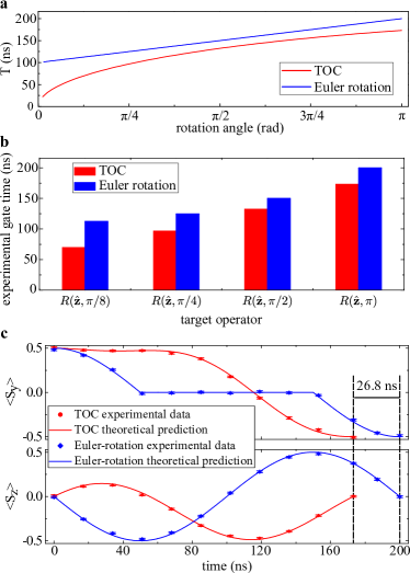
Figure 2: (color online). Comparison on time costs for target gate operator $R(\hat{\mathbf{z}},\theta)$ between the derived TOC and the Euler rotations. The parameters are set to be $\delta=0$ and $\nu_{1}=5$ MHz. (a) Theoretical comparison on time with $\theta\in(0,\pi]$. (b) Comparison of experimental gate time for $\theta=\pi/8,\pi/4,\pi/2,$ and $\pi$. The gate time for TOC is considerably shorter than that for Euler rotation. (c) State evolutions during $R(\hat{\mathbf{z}},\pi)$ with TOC and Euler rotation. The initial state is $(|m_{s}=0\rangle+i|m_{s}=-1\rangle)/\sqrt{2}$. The gate time of TOC is 26.8 ns shorter than that of Euler rotation.

The realization of a target $R(\hat{\mathbf{z}},\theta),\theta\in(0,\pi]$ when $\delta=0$ is taken as an example to compare the time cost between the derived TOC and a non-optimized evolution path with Euler rotation: $R(\hat{\mathbf{z}},\theta)=R(\hat{\mathbf{x}},\pi/2)R(\hat{\mathbf{y}},\theta)R(-\hat{\mathbf{x}},\pi/2)$. The experimental amplitude of control field is set to be $\nu_{1}=5$ MHz. Theoretical comparison of the time cost for gate operations between TOC and Euler rotation is shown in Fig. 2a. It is clear that the time cost with TOC is considerably shorter than that with Euler rotation for all the rotation angles. We experimentally implement the target gate operators $R(\hat{\mathbf{z}},\pi/8)$, $R(\hat{\mathbf{z}},\pi/4)$, $R(\hat{\mathbf{z}},\pi/2)$, and $R(\hat{\mathbf{z}},\pi)$ with both methods. Figure 2b shows the comparison of the experimental gate time. The time durations for gate operations with TOC are 69.6, 96.8, 132.3, and 173.2 ns, which are 42.9, 28.1, 17.7, and 26.8 ns shorter than those with Euler rotation, respectively. Figure 2c shows the state evolution during $R(\hat{\mathbf{z}},\pi)$. The initial state is prepared to $(|m_{s}=0\rangle+i|m_{s}=-1\rangle)/\sqrt{2}$. We performed measurements of $\langle S_{y}\rangle$ and $\langle S_{z}\rangle$ on the states during the evolution. As shown in Fig. 2c, the target evolution of $R(\hat{\mathbf{z}},\pi)$ is realized at 173.2 ns with TOC and at 200 ns with Euler rotation. All the gate fidelities PLA_Nielsen are measured to be above 0.99 via quantum process tomography Nielsen .

The case when $\delta\neq 0$ has also been experimentally implemented. Both $R(\hat{\mathbf{z}},\theta)$ and $R(\hat{\mathbf{x}},\theta)$ with various values of $\theta$ have been demonstrated. Furthermore, time-optimal universal single-qubit control with other constraints on $H_{c}$ is also experimentally demonstrated. The implementations are characterized utilizing quantum process tomography (see Section III in Supplementary Material). The experimental results for the cases are presented in Section II, Fig. S3, Fig. S4, and TABLE I of the Supplementary Material. Our results show the universality of our approach to perform time-optimal universal control for a single qubit.

Universal control of qubits also requires a non-trivial two-qubit gate JAJones . In our experiment, we demonstrate a controlled-U gate with

$$U_{c}=\left(\begin{array}[]{cccc}1&0&0&0\\ 0&0&0&1\\ 0&0&1&0\\ 0&-1&0&0\\ \end{array}\right),$$ (2)

which is also a non-trivial two-qubit gate JAJones . In our experiment, we have demonstrated this two-qubit gate in a time-optimal way with the system consisting of the electron and nuclear spins. Electron (nuclear) spin states $|m_{S}=0\rangle$ and $|m_{S}=-1\rangle$ ($|m_{I}=+1\rangle$ and $|m_{I}=0\rangle$) are encoded as the electron (nuclear) spin-qubit. The quantum state of the two-qubit system is denoted as $|m_{S},m_{I}\rangle$, with corresponding population denoted as $P_{m_{S},m_{I}}$ hereafter. The drift Hamiltonian, $H_{0}=2\pi AS_{z}I_{z}$, is the hyperfine coupling between the spins, where $I_{z}$ is the effective spin operator of the nuclear spin qubit and the hyperfine coupling strength is $A=-2.16~{}$MHz. We consider a model in which only controls with bounded strength on the electron spin are applied, while the control Hamiltonian takes the form $H_{c}(t)=2\pi\nu_{1}[\cos\phi(t)S_{x}+\sin\phi(t)S_{y}]$. The strength of the control field $\nu_{1}$ is set to $2.5~{}$MHz. The constraints on the control Hamiltonian can be described by $f_{0}(H_{c})=0$ and $f_{k}(H_{c})\equiv Tr(H_{c}B_{k})=0$, where $\{B_{k}\}=\{I_{x},I_{y},I_{z},S_{x}I_{x},S_{x}I_{y},S_{x}I_{z},S_{y}I_{x},S_{y}I_{y},S_{y}I_{z},S_{z},S_{z}I_{x},\\ S_{z}I_{y},S_{z}I_{z}\}$. The target evolution operator is a controlled unitary gate which flips the electron spin qubit iff the nuclear spin qubit is in the state $|m_{I}=0\rangle$. The time-optimal control Hamiltonian is obtained by numerically solving the QBE together with the Schrödinger equation (see Section II in Supplementary Material). If the dephasing effect and the imperfection of the control field are taken into account NatCommun_Du , the theoretical fidelity of $U_{c}$ is estimated to be $0.9933$. The detailed experimental pulse for time-optimal control and the fidelity estimation are included in Section II and Fig. S5 in Supplementary Material. The time duration of the controlled-U gate with TOC is 446 ns. A conventional method to implement the controlled-U gate with the constraint control field is to apply a selective pulse PRA_Dorai ; JMR_Mahesh . With $\nu_{1}=2.5$ MHz (the same as that in TOC), the time duration to implement the controlled-U gate with a selective pulse is 612.4 ns (see Section II in Supplementary Material), which is more than 160 ns longer than that with TOC.

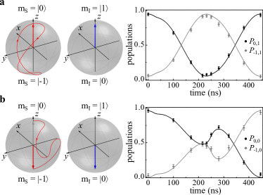
Figure 3: (color online). State trajectories under the two-qubit controlled-U gate by TOC with initial states (a) $|0,1\rangle$ and (b) $|0,0\rangle$. The left panels show the state evolutions of the nuclear and electron spins on the Bloch spheres. When the nuclear spin qubit is in the state $|1\rangle$ ($|0\rangle$) labeled by the blue arrows, the electron spin qubit undergoes the paths labeled by red lines to the state $|0\rangle$ ($|-1\rangle$). The right panels show the experimental dynamics of state populations $P_{0,m_{I}}$ (black circles) and $P_{-1,m_{I}}$ (grey diamonds), and lines are theoretical predictions of the populations. The error bars on the data points are the standard deviations from the mean.

Figure 3 shows the state evolutions under $U_{c}$ via TOC. In Fig. 3a and b, the initial states are prepared into $|0,1\rangle$ and $|0,0\rangle$, respectively. The left panel of Fig. 3a (b) shows the state trajectory of the electron spin qubit on the Bloch sphere, while the nuclear spin state is $|m_{I}=+1\rangle$ ($|m_{I}=0\rangle$). It is clear that the electron spin qubit is flipped to the state $|-1\rangle$ with the nuclear spin qubit in $|m_{I}=0\rangle$, and the state of the electron spin qubit returns to the state $|0\rangle$ with the nuclear spin qubit in $|m_{I}=+1\rangle$. In the right panels of Fig. 3a and b, experimental populations of $|0,m_{I}\rangle$ and $|-1,m_{I}\rangle$ (i.e., $P_{0,m_{I}}$ and $P_{-1,m_{I}}$) during the $U_{c}$ gate are recorded. The experimental results represented by symbols are in agreement with theoretical predictions represented as lines. The small deviation from $1$ ($0$) of $P_{0,m_{I}}$ ($P_{-1,m_{I}}$) at $t=0$ is due to imperfect polarization of the electron spin (about 0.95, which is measured with sequences described in Section IV and Fig. S6 in Supplementary Material).

We further perform quantum process tomography (see Section III in Supplementary Material) to characterize the $U_{c}$ gate. A set of 16 initial states is prepared, after which the $U_{c}$ is applied, and quantum state tomography is applied to reconstruct the final state corresponding to each initial state. With the information of the $16$ final states, the process matrix $\chi$ is determined in the Pauli basis $\{\sigma_{i}\otimes\sigma_{j}\}$, where $\sigma_{i(j)}\in\{I,X,Y,Z\}$, $I$ is the identity operator, and $X=\sigma_{x}$, $Y=\sigma_{y}$, and $Z=\sigma_{z}$ are Pauli operators. Figure 4 shows the real and imaginary parts of the experimental process matrix. The average gate fidelity of the two-qubit gate in our experiment is $0.99(1)$, which reaches the threshold of fault-tolerant quantum computations Nature_Barends . The shortest possible time duration of the gate operation by TOC is advantageous to high fidelity due to the reduction of the dephasing effect. The relatively small strength of the control field also contributes to the high fidelity, as the noise induced from the control field is proportional to the control field NatCommun_Du ; PRL_Du .

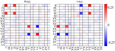
Figure 4: (color online). Quantum process tomography for controlled-U gate by TOC. The left and right panels are the real and imaginary parts of the reconstructed process matrix $\chi$. The error bar of each point is about $0.01$ due to the statistics of photon counts. An average gate fidelity of 0.99(1) can be obtained from the process matrix.

Discussion.—Manipulation of quantum systems is of fundamental significance in quantum computing Nielsen , quantum metrology PRL_Giovannetti , and high-resolution spectroscopy Nature_Maze ; Nature_Balasubramanian ; Science_Schmidt_2005 . It is desirable to achieve universal control with high fidelity and in a minimal time interval in the presence of decoherence. High fidelity universal control has been reported in various quantum systems, including trapped ions Natphy_Benhelm , superconducting circuits Nature_Barends , NV centers in diamond Nature_Hanson ; NatCommun_Du , and spins in silicon Nature_Veldhorst ; Nature_Pla . However, experimental demonstration of universal control, when high fidelity and minimal time are satisfied simultaneously, were not achieved in previous work. We have realized the time-optimal universal control of the two-qubit system in diamond with high fidelity. Our results provide an experimental validation of TOC casting a high-fidelity control operation on multi-qubit systems. The approach developed in this work to realize accurate minimum time control of multiqubits can be applied to other important physical systems.

We are grateful to C. K. Duan and C. Y. Ju for valuable discussions. This work was supported by the National Basic Research Program of China (Grants No. 2013CB921800 and No. 2016YFB0501603), the National Natural Science Foundation of China (Grants No. 11227901, No. 31470835, and No. 11275183) and the Strategic Priority Research Program (B) of the CAS (Grant No. XDB01030400). F.S. and X.R. thank the Youth Innovation Promotion Association of Chinese Academy of Sciences for support. X. W. is supported by NSF project No. CCF-1350397.

J. G. and Y. W. contributed equally to this work.

Supplmentary Material

I I. Hamiltonian of the NV system

The Hamiltonian of the NV center can be written as

$$H_{NV}=2\pi(DS_{z,3}^{2}+\omega_{S}S_{z,3}+PI_{z,3}^{2}-\omega_{I}I_{z,3})+H_{hf},$$ (EqS1)

where $\omega_{S}=-\gamma_{e}B_{0}/2\pi(\omega_{I}=\gamma_{N}B_{0}/2\pi)$ is the Zeeman splitting of the electron (¹⁴N nuclear) spin, $\gamma_{e}(\gamma_{N})$ is the electronic (¹⁴N nuclear) gyromagnetic ratio, $S_{z,3}$ and $I_{z,3}$ are the electron and nitrogen nuclear spin operators of spin-1 systems. The zero field splitting $D=2870$ MHz and the nuclear quadrupolar splitting $P=-4.95$ MHz. The hyperfine interaction between the NV electron and the ¹⁴N nuclear spin is

$$H_{hf}=2\pi[A_{\perp}(S_{x,3}I_{x,3}+S_{y,3}I_{y,3})+AS_{z,3}I_{z,3}],$$ (EqS2)

where $A=-2.16$ MHz. Because of the strong zero field splitting and Zeeman splitting terms of the electron spin, the effect of the interaction term $S_{x,3}I_{x,3}+S_{y,3}I_{y,3}$ can be neglected. In the secular approximation, the Hamiltonian is

$$H_{NV}=2\pi(DS_{z,3}^{2}+\omega_{S}S_{z,3}+AS_{z,3}I_{z,3}+PI_{z,3}^{2}-\omega_{I}I_{z,3}),$$ (EqS3)

The spin energy levels of the NV center are shown in Fig. S1. The electron (nuclear) spin states $|m_{S}=0\rangle$ and $|m_{S}=-1\rangle$ ($|m_{I}=1\rangle$ and $|m_{I}=0\rangle$) are encoded as the electron (nuclear) spin qubit. The Hamiltonian can be simplified to that of a two-qubit system.

Figure S1: Spin energy level diagram of the NV center. The experiments are implemented on the two-qubit system composed with the energy levels boxed with dashed lines (i.e. $|m_{S}=0,m_{I}=1\rangle$, $|m_{S}=0,m_{I}=0\rangle$, $|m_{S}=-1,m_{I}=1\rangle$, and $|m_{S}=-1,m_{I}=0\rangle$).

In the single-qubit case, the experiments are implemented on the electron spin qubit while the nuclear spin is kept in state $|m_{I}=1\rangle$. When microwave (MW) pulses with the frequency of $f_{MW}$ are applied, the total Hamiltonian of the electron spin qubit is

$$H_{1}=2\pi(-(D-\omega_{S}-A)S_{z}+2\nu_{1}\cos(2{\pi}f_{MW}t-\phi)S_{x}),$$ (EqS4)

where $\phi$ is the phase of the MW pulse, $\nu_{1}$ is the amplitude of the MW pulse, $S_{x}$, $S_{y}$, and $S_{z}$ are electron spin operators of a spin-1/2 system. The Hamiltonian can be transformed into the rotating frame as

$$H_{rot1}=U_{trans1}H_{1}U_{trans1}^{\dagger}-iU_{trans1}\frac{dU_{trans1}^{\dagger}}{dt},$$ (EqS5)

with

$$U_{trans1}=e^{-i2{\pi}f_{MW}tS_{z}}.$$ (EqS6)

With rotating-wave approximation, the Hamiltonian in the rotating frame can be simplified as

$$H_{rot1}=2{\pi}({\delta_{0}}S_{z}+\nu_{1}(\cos\phi S_{x}+\sin\phi S_{y})),$$ (EqS7)

where $\delta_{0}=-(D-\omega_{S}-A-f_{MW})$.

The two-qubit experiments are implemented on the two-qubit system comprised with the electron and nuclear spin qubits. The two-qubit states can be manipulated with MW and radio-frequency (RF) pulses. The frequency of the RF pulse is denoted by $f_{RF}$. When only MW pulses are applied, the total Hamiltonian is

$$H_{2}=2\pi(-(D-\omega_{S}-A/2)S_{z}+(P-\omega_{I}-A/2)I_{z}+AI_{z}S_{z}+2\nu_{1}\cos(2{\pi}f_{MW}t-\phi)S_{x}),$$ (EqS8)

where $I_{x}$, $I_{y}$, $I_{z}$ are nuclear spin operators of a spin-1/2 system. The Hamiltonian can be transformed into the rotating frame as

$$H_{rot2}=U_{trans2}H_{2}U_{trans2}^{\dagger}-iU_{trans2}\frac{dU_{trans2}^{\dagger}}{dt},$$ (EqS9)

with

$$U_{trans2}=e^{-i2{\pi}f_{MW}tS_{z}}e^{-i2{\pi}f_{RF}tI_{z}}.$$ (EqS10)

With rotating-wave approximation, the Hamiltonian in the rotating frame can be simplified as

$$H_{rot2}=2\pi[AS_{z}I_{z}+\nu_{1}(\cos{\phi}S_{x}+\sin{\phi}S_{y})],$$ (EqS11)

with $f_{MW}=D-\omega_{S}-A/2$, $f_{RF}=-P+\omega_{I}+A/2$.

II II. Time-optimal control with quantum brachistochrone equation

The goal of quantum time-optimal control (TOC) is to complete the quantum control task(e.g., to generate a unitary gate or to prepare an entangled state) in the shortest time. In general, there are two constraints for the quantum TOC problem: (i) due to the finite energy bandwidth of the quantum system, its evolution under the Schrödinger equation cannot be arbitrarily fast; (ii) the Hamiltonian of a realistic quantum device usually takes a given form, and the way we can vary the Hamiltonian must satisfy this form, implying we cannot generate arbitrary quantum trajectory. Under these two constraints, it has been found that the quantum TOC problem can be solved by solving the so-called quantum brachistochrone equation (QBE) PRL_Carlini_S ; PRA_Carlini_S .

Specifically, let $H(t)$ be the Hamiltonian of the quantum device that can be varied over time. In the most general case, $H(t)=H_{0}+H_{c}(t)$, where $H_{0}$ is known as the drift term which cannot be varied over time (e.g., $H_{0}=2\pi AS_{z}I_{z}$ in (EqS11)), and $H_{c}$ is the control Hamiltonian in a fixed form (e.g., $H_{c}(t)=2\pi\nu_{1}(\cos{\phi(t)}S_{x}+\sin{\phi(t)}S_{y})$ in (EqS11)). Then the above two constraints can be expressed as the following:
(i) $f_{0}(H)\equiv||H_{c}(t)||^{2}-E^{2}=\operatorname{Tr}(H_{c}^{2}(t))-E^{2}=0$
(ii) $f_{k}(H)\equiv\operatorname{Tr}(H_{c}(t)B_{k})=0,\text{ where }k=1,\cdots,m$
where $\{B_{k}\}$ is a basis of the matrix subspace $\mathcal{Q}$ satisfying $\operatorname{Tr}(H_{c}(t)\mathcal{Q})=0$. Notice that, in principle, the constraint for finite energy bandwidth should be expressed as the inequality (i’) $||H_{c}(t)||^{2}\leq E^{2}$, but we find that (i’) leads to (i) in many cases, including the problems discussed in this work.

For the gate generation problem, the objective is to find the appropriate control Hamiltonian $H_{c}(t)$ such that the evolution $U(t)$ under the Schrödinger equation $\dot{U}=-iH(t)U$ satisfies $U(0)=I$ and $U(T)=U_{F}$, where $U_{F}$ is the target unitary and $T$ is the total evolution time. This control solution $(H(t),U(t))$ is not unique, and numerically we can use optimization method to find many such solutions. However, if the control objective also requires the total time $T$ to be minimized, then the time-optimal control can be mathematically characterized: defining the Lagrangian $\mathcal{L}$ under the constraints (i) and (ii), the time-optimal solution $(H(t),U(t))$ must satisfy the Euler-Lagrange equation for $\mathcal{L}$:

$$\dot{F}=-i[H,F],$$ (EqS12)

where $L_{c}\equiv\sum_{j}\lambda_{j}f_{j}(H)$, $j=0,1\cdots m$, $\lambda_{j}$ are Lagrange multipliers and $F=\frac{\partial L_{c}}{\partial H}=\frac{\partial L_{c}}{\partial H_{c}}$ since $H_{0}$ is constant.

Since the QBE is a first-order ordinary differential equation (ODE), in order to solve the time-optimal gate generation problem for $U_{F}$, it is sufficient to find the initial value $(H(0),\lambda_{j}(0))$ satisfying $U(T)=U_{F}$. This is a boundary value nonlinear problem. Except a few special cases where analytic solutions exist, one has to resort numerical method to solve it. Unfortunately, the standard method (e.g. the shooting method) of numerically solving a boundary value nonlinear equation soon becomes inefficient as the dimension of the problem grows. This forces us to think of new method to solve the QBE.

Fortunately, for the special case where $H_{0}=0$, the QBE has an intuitive geometric interpretation, i.e., it can be considered as the limit of a family of 1-parameter geodesics under the so-called $q$-metric PRL_Wang_S . Such brachistochrone-geodesic connection provides a very efficient way of solving the QBE even for the system with a large dimension. Analogously, for the more general case where $H_{0}\neq 0$, we can develop a similar method to solve the QBE.

Specifically, let $\mathcal{P}$ be the matrix subspace where $H_{c}(t)$ can choose values in, so we have $\operatorname{Tr}(\mathcal{P}\mathcal{Q})=0$. Notice that the key point to solve the first-order QBE (EqS12) is to find a good guess of the initial value $(H_{c}(0),\lambda_{j}(0))$. This can be achieved by the following approach:

First, assume $H_{c}(t)$ is only chosen from the control space $\mathcal{P}$. The time-optimal problem is equivalent to solving the following two-objective optimization problem: maximizing the fidelity of evolution operator with the target operator, $\mathrm{Fi}(U(T),U_{F})$, and minimizing the evolution time, $T=\int_{0}^{T}dt$. Meanwhile, the control Hamiltonian is subjected to the constraint $||H_{c}(t)||=E$. In order to solve it, we can use weighted summation to convert the two-objective problem into a single-objective minimization problem ($\kappa>0$), with the objective function:

$$J=-\mathrm{Fi}(U(T),U_{F})+\kappa\int_{0}^{T}dt$$ (EqS13)

We expect that this combined optimization problem will give us a reasonably good approximation of time-optimal solution $H_{c}(t)$. Thus, we can get a good guess for $H_{c}(0)$, but this is not sufficient to solve the QBE, as the initial values for the Lagrange multipliers $\lambda_{j}(0)$ are still unknown.

To overcome this problem, we introduce a family of 1-parameter brachistochrone equations under the $q$-metric, which is similar to the family of the geodesic equations in Ref. PRL_Wang_S, . In this frame, the time-optimal curves are reformulated in the following way: allowing the control Hamiltonian $H_{c}(t)$ to take components from both $\mathcal{P}$ and $\mathcal{Q}$ but with a penalty when taking components from $\mathcal{Q}$. Specifically, we define the $q$-norm, characterizing the penalty: $||H_{c}||_{q}^{2}=||\mathcal{P}(H_{c})||^{2}+q||\mathcal{Q}(H_{c})||^{2}$, $q\geq 1$, where $\mathcal{P}(H_{c})$ ($\mathcal{Q}(H_{c})$) indicate the projection of $H_{c}$ in subspace $\mathcal{P}$ ($\mathcal{Q}$). Then we study the time-optimal solution under the following constraint: $||H_{c}||_{q}=E$. As $q\to+\infty$, the component of $H_{c}(t)$ on the subspace $\mathcal{Q}$ decreases to zero, we will recover the brachistochrone equation for the original problem. Thus, we can solve the weighted-sum optimization problem shown in (EqS13), with the constraint $||H_{c}(t)||_{q}=E$. The optimal solution provides a good initial guess of $(H_{c}(0),q\lambda_{j}(0))$, which can be used to find the solution of the $q$-metric brachistochrone equation for $q\gg 1$, which then provides a good guess to solve the original QBE. The detailed procedure is similar to that in the Ref. PRL_Wang_S, .

II.1 A. Single-qubit case

The entire Hamiltonian is $H(t)=H_{0}+H_{c}(t)$, with $H_{0}=2\pi{\delta}S_{z}$ and $H_{c}(t)=2\pi\nu_{1}[\cos\phi(t)S_{x}+\sin\phi(t)S_{y}]$. The target operator is $U_{F}=R(\hat{\mathbf{n}},\theta)\equiv\exp(-i\theta\hat{\mathbf{n}}\cdot\textbf{S})$, with $\hat{\mathbf{n}}=\hat{\mathbf{x}}\sin\gamma\cos\varphi+\hat{\mathbf{y}}\sin\gamma\sin\varphi+\hat{\mathbf{z}}\cos\gamma$ being a unit vector. From QBE, we have $\phi(t)=2\pi\eta t+\phi_{0}$. The parameter $\eta$ characterizing the control Hamiltonian and the minimum evolution time $T$ can be obtained by solving the Schrödinger equation with boundary conditions. The solution to the Schrödinger equation reduces the boundary conditions to the following equations.

$$\left\{\begin{aligned} &\cos(\pi\eta T)\cos(\pi\sqrt{\nu_{1}^{2}+(\delta-\eta)^{2}}T)\\ &~{}~{}~{}~{}~{}~{}~{}-\sin(\pi\eta T)\sin(\pi\sqrt{\nu_{1}^{2}+(\delta-\eta)^{2}}T)\frac{\delta-\eta}{\sqrt{\nu_{1}^{2}+(\delta-\eta)^{2}}}=\pm\cos\frac{\theta}{2}\\ &\sin(\pi\eta T)\cos(\pi\sqrt{\nu_{1}^{2}+(\delta-\eta)^{2}}T)\\ &~{}~{}~{}~{}~{}~{}~{}+\cos(\pi\eta T)\sin(\pi\sqrt{\nu_{1}^{2}+(\delta-\eta)^{2}}T)\frac{\delta-\eta}{\sqrt{\nu_{1}^{2}+(\delta-\eta)^{2}}}=\pm\cos\gamma\sin\frac{\theta}{2}\\ &\frac{\nu_{1}}{\sqrt{\nu_{1}^{2}+(\delta-\eta)^{2}}}\cos(\pi\eta T+\phi_{0})\sin(\pi\sqrt{\nu_{1}^{2}+(\delta-\eta)^{2}}T)=\pm\sin\gamma\cos\varphi\sin\frac{\theta}{2}\\ &\frac{\nu_{1}}{\sqrt{\nu_{1}^{2}+(\delta-\eta)^{2}}}\sin(\pi\eta T+\phi_{0})\sin(\pi\sqrt{\nu_{1}^{2}+(\delta-\eta)^{2}}T)=\pm\sin\gamma\sin\varphi\sin\frac{\theta}{2}\end{aligned}\right.$$ (EqS14)

As an example, we give analytic solution to $U_{F}=R(\hat{\mathbf{z}},\theta),\theta\in(0,2\pi)$. Without loss of generality, $\delta\geq 0$ and $\nu_{1}>0$ is supposed.

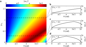
Figure S2: Analytic solution of single-qubit TOC for target evolution operator $R(\hat{\mathbf{z}},\theta)$. (a) The minimum evolution time analytically calculated from QBE with $H_{c}\in\mathrm{span}\{S_{x},S_{y}\}$ and target evolution operator $R(\hat{\mathbf{z}},\theta)$ with $\theta\in[0,2\pi)$. (b - d) show the minimum evolution time as a function of rotation angle for different ratios between $\delta$ and $\nu_{1}$.

When $\theta<\pi(1+\sqrt{3}\delta/\nu_{1})$

$$T=\frac{\delta(\frac{\theta}{2\pi}-1)+\sqrt{\nu_{1}^{2}+\delta^{2}-\nu_{1}^{2}(\frac{\theta}{2\pi}-1)^{2}}}{\nu_{1}^{2}+\delta^{2}}$$ (EqS15)

$$\eta=-\frac{2\pi-\theta}{2\pi T}.$$ (EqS16)

When $\theta\geq\pi(1+\sqrt{3}\frac{\delta}{\nu_{1}})$

$$T=\frac{\delta\frac{\theta}{2\pi}+\sqrt{\nu_{1}^{2}+\delta^{2}-\nu_{1}^{2}(\frac{\theta}{2\pi})^{2}}}{\nu_{1}^{2}+\delta^{2}}$$ (EqS17)

$$\eta=-\frac{\theta}{2\pi T}.$$ (EqS18)

The minimum time $T$ as a function of $\theta$ and $\delta/\nu_{1}$ (equation EqS15 and EqS17) is shown in Fig. S2. When $\delta=0$, our result reduces to that in Ref. PRA_Boozer_S, . In this case, we compare the time duration with TOC and that with Euler rotation. The experimental results is shown in the main text.

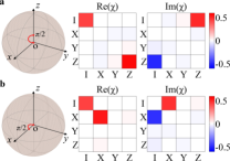
Figure S3: Experimental implementation of single-qubit TOC for target evolution operators (a) $R(\hat{\mathbf{z}},\pi/2)$ and (b) $R(\hat{\mathbf{x}},\pi/2)$. The left panels show the time-optimal evolution paths. The spheres in the left column stand for the rotation groupPRL_Meier_S . The center of the sphere O stands for the identity gate operation. The direction of the vector joining the center O to any other point represents the axis of rotation, whereas the length of the vector represents the angle of rotation. The right panels are experimental operations characterized by quantum process tomography. The results show average gate fidelities of (a) 1.00(1) and (b) 0.99(1), respectively.

Then we experimentally demonstrate the case of $\delta\not=0$. In this experiment we set $\delta=1.5~{}$MHz and $\nu_{1}=5~{}$MHz. To visualize the evolution path of the TOC, the evolution operator $R(\hat{\mathbf{n}},\theta)$ is mapped to the point $(\theta\sin\gamma\cos\varphi,\theta\sin\gamma\sin\varphi,\theta\cos\gamma)$ in a three-dimensional frame of $\theta\in[0,2\pi]$. All single-qubit evolution operators can be mapped to points within the sphere with radius of $2\pi$ PRL_Meier_S . The time-optimal evolution paths of the TOC for target evolution operators $R(\hat{\mathbf{z}},\pi/2)$ and $R(\hat{\mathbf{x}},\pi/2)$ are represented in the left panels of Fig. S3a and b, respectively. To characterize the performance of the TOC, quantum process tomography Nielsen_S is utilized (see Section III). The reconstructed process matrices for $R(\hat{\mathbf{z}},\pi/2)$ and $R(\hat{\mathbf{x}},\pi/2)$ are shown in the right panels of Fig. S3a and b, respectively. The corresponding average gate fidelities PLA303_249_S are measured to be $1.00(1)$ and $0.99(1)$.

We further exhibit the state evolutions during the time-optimal $R(\hat{\mathbf{z}},\pi/2)$ and $R(\hat{\mathbf{x}},\pi/2)$. The initial state is prepared to $|m_{S}=0\rangle$. State populations of $|m_{S}=0\rangle$ during the evolutions are recorded. As shown in Fig. S4, experimental results are in great agreement with theoretical predictions.

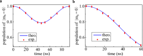
Figure S4: State evolution under (a) $R(\hat{\mathbf{z}},\pi/2)$ and (b) $R(\hat{\mathbf{x}},\pi/2)$ by single-qubit TOC with initial state $|m_{s}=0\rangle$. The control Hamiltonian $H_{c}\in\mathrm{span}\{S_{x},S_{y}\}$, with other parameters set to be $\delta=1.5$ MHz, $\nu_{1}=5$ MHz. The symbols are experimentally recorded state population of $|m_{S}=0\rangle$, and solid lines are theoretical predictions. The error bars on the data points are the standard deviations from the mean.

In addition to the experiments mentioned above, more single-qubit gate operators with TOC are experimentally demonstrated. Our method also applies to TOC with other constraints on $H_{c}$ (e.g. $H_{c}(t){\in}\mathrm{span}\{S_{x},S_{y},S_{z}\}$). We also implement single-qubit TOC with constraint $H_{c}(t){\in}\mathrm{span}\{S_{x},S_{y},S_{z}\}$. All the experimental results are summarized in TABLE 1. Our results show the universality of our approach to perform time-optimal universal control for single qubit.

Table 1: Summarization of the results of single-qubit TOC. Average gate fidelity ($F_{\textrm{a}}$) and evolution time ($T\mathrm{(ns)}$) is shown for different cases with experimental parameter $\nu_{1}=5$ MHz.

$\delta/\nu_{1}$	Control space	Target operator	$F_{\textrm{a}}$	$T\mathrm{(ns)}$
$\delta/\nu_{1}=0$	$H_{c}\in\mathrm{span}\{S_{x},S_{y}\}$	$R(\hat{\mathbf{z}},\pi/2)$	0.99(1)	132.3
		$R(\hat{\mathbf{z}},5\pi/4)$	0.98(1)	156.1
		$R(\hat{\mathbf{z}},7\pi/4)$	0.98(1)	96.8
$\delta/\nu_{1}=0.3$	$H_{c}\in\mathrm{span}\{S_{x},S_{y},S_{z}\}$	$R(\hat{\mathbf{z}},\pi/2)$	0.99(1)	38.5
		$R(\hat{\mathbf{z}},5\pi/4)$	0.98(1)	96.2
		$R(\hat{\mathbf{z}},7\pi/4)$	0.99(1)	35.7
		$R(\hat{\mathbf{x}},\pi/4)$	0.98(1)	26.1
		$R(\hat{\mathbf{x}},\pi/2)$	0.99(1)	51.9
	$H_{c}\in\mathrm{span}\{S_{x},S_{y}\}$	$R(\hat{\mathbf{z}},\pi/2)$	1.00(1)	92.0
		$R(\hat{\mathbf{z}},5\pi/4)$	0.98(1)	158.1
		$R(\hat{\mathbf{z}},7\pi/4)$	0.99(1)	152.7
		$R(\hat{\mathbf{x}},\pi/4)$	0.98(1)	63.2
		$R(\hat{\mathbf{x}},\pi/2)$	0.99(1)	59.6
$\delta/\nu_{1}=1.1$	$H_{c}\in\mathrm{span}\{S_{x},S_{y},S_{z}\}$	$R(\hat{\mathbf{z}},\pi/2)$	0.99(1)	23.8
		$R(\hat{\mathbf{z}},5\pi/4)$	0.99(1)	59.5
		$R(\hat{\mathbf{z}},7\pi/4)$	0.99(1)	83.3
		$R(\hat{\mathbf{x}},\pi/4)$	0.99(1)	95.4
		$R(\hat{\mathbf{x}},\pi/2)$	0.98(1)	96.0
	$H_{c}\in\mathrm{span}\{S_{x},S_{y}\}$	$R(\hat{\mathbf{z}},\pi/2)$	0.99(1)	41.5
		$R(\hat{\mathbf{z}},5\pi/4)$	0.98(1)	92.9
		$R(\hat{\mathbf{z}},7\pi/4)$	0.99(1)	121.6
		$R(\hat{\mathbf{x}},\pi/4)$	0.98(1)	122.9
		$R(\hat{\mathbf{x}},\pi/2)$	0.99(1)	111.7

II.2 B. Two-qubit case

We exhibit the approach to obtain the time-optimal control of two-qubit system in NV center. The drift Hamiltonian is the hyperfine coupling between electron and nuclear spin qubits. The system is steered by control pulse on the electron spin-qubit with finite strength. Thus, $H_{0}=2\pi{A}S_{z}I_{z}$ and $H_{c}(t)=2\pi\nu_{1}[\cos\phi(t)S_{x}+\sin\phi(t)S_{y}]$. The hyperfine coupling strength is $A=\mathrm{-2.16}$MHz. The strength of the control field $\nu_{1}$ is set to 2.5 MHz. The constraints on the control Hamiltonian can be described by $f_{0}(H)=0$ and $f_{k}(H)=0$, where $\{B_{k}\}=\{I_{x},I_{y},I_{z},S_{x}I_{x},S_{x}I_{y},S_{x}I_{z},S_{y}I_{x},S_{y}I_{y},S_{y}I_{z},S_{z},S_{z}I_{x},S_{z}I_{y},S_{z}I_{z}\}$. The target evolution operator is a controlled-U gate which flips the electron spin qubit iff the nuclear spin is in state $|m_{I}=0\rangle$. The form of this gate is shown in equation 2 in the main text. This gate is a non-trivial two-qubit gate JAJones_S , which can convert a product state to an entangled state.

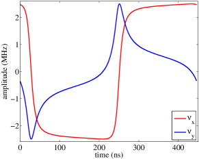
Figure S5: Pulse sequence for non-trivial two-qubit gate, $U_{c}$, via TOC in NV system. The amplitude of the control pulse is $\nu_{1}=2.5$ MHz. The x- and y-components of the control amplitude are denoted by $\nu_{x}$ and $\nu_{y}$.

The time-optimal control Hamiltonian $H_{c}(t)$ can be numerically obtained by steps mentioned above, with $\mathcal{P}=$span$\{S_{x},S_{y}\}$, $\mathcal{Q}=$span$\{B_{k}\}$ and $q=1000$. Figure S5 shows the time-optimal pulse sequence, where $\nu_{x}={\nu_{1}}\cos\phi(t)$ and $\nu_{y}={\nu_{1}}\sin\phi(t)$ are x- and y-components of the control amplitude. Although the time-optimal sequence is derived for a closed system, high fidelity is expected when applying it to realistic systems. For example, if considering dephasing effect and imperfection of control field NatCommun_Du_S , an fidelity of 0.9933 is estimated. The high fidelity benefits from the least possible accumulation of errors during the shortest possible time, which is 446.1 ns.

We compare the time duration of controlled-U gate with TOC and that with a conventional method of applying a selective pulsePRA_Dorai_S ; JMR_Mahesh_S . The frequency of the pulse is matched to the energy difference between $|m_{S}=0,m_{I}=0\rangle$ and $|m_{S}=-1,m_{I}=0\rangle$. By choosing an appropriate control strength, the controlled-U gate can be realized with conditional rotation of the electron spin, i.e. a rotation of $(2k_{1}+1)\pi$ for $|m_{I}=0\rangle$ and $2k_{2}\pi$ for $|m_{I}=1\rangle$, where $k_{1}$ and $k_{2}$ are integers. With $\nu_{1}=2.5$ MHz, the controlled-U gate can be realized by $k_{1}=1$ and $k_{2}=2$. The time duration with this method is 612.4 ns, which is more than 160 ns longer than that with TOC.

III III. Quantum process tomography

We use standard quantum process tomography Nielsen_S to evaluate the experimentally realized quantum gates. An unknown process $\mathcal{E}$ acting on the initial state $\rho$ and generating the final state ${\mathcal{E}}(\rho)$ can be described as

$$\mathcal{E}(\rho)=\sum_{m,n=1}^{d^{2}}\chi_{mn}A_{m}{\rho}A_{n}^{\dagger},$$ (EqS19)

where $A_{m}\in SU(d)$ represents a full set of orthogonal basis operators and $\chi_{mn}$ is the coefficient of the process matrix $\chi$ which completely describes the process $\mathcal{E}$. In our experiments the process matrix $\chi$ is determined in the Pauli basis $A_{n}$, where $A_{n}=\{\sigma_{i}\}$ for single-qubit case and $A_{n}=\{\sigma_{i}\otimes\sigma_{j}\}$ for two-qubit case, $\sigma_{i(j)}\in\{I,X,Y,Z\}$, and $I$ is the identity operator, $X=\sigma_{x}$, $Y=\sigma_{y}$, and $Z=\sigma_{z}$ are Pauli operators. We prepare a complete set of basis states $\rho_{1}\ldots\rho_{d^{2}}$ with microwave (MW) and radio frequency (RF) pulses. The MW pulse is applied after RF pulse to depress the decoherence of the electron spin in the preparation of two-qubit initial states. The fidelity of the quantum process is then given by the average gate fidelity PLA303_249_S ,

$$F_{\textrm{a}}(\mathcal{E},U)=\frac{\sum_{j}\mathrm{tr}(UU_{j}^{\dagger}U^{\dagger}\mathcal{E}(U_{j}))+d^{2}}{d^{2}(d+1)},$$ (EqS20)

where $U$ is the theoretically ideal transformation and $U_{j}$ is a basis of unitary operators.

IV IV. Normalization of the experimental data

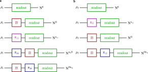
Figure S6: Schematic normalization sequences in the two-qubit experiment. Here $\rho_{\textrm{i}}$ denotes the initialized state after a laser pulse, $\rho_{\textrm{f}}$ denotes the final state after applying control sequence to $\rho_{\textrm{i}}$. $\pi_{12}$ ($\pi_{34}$) is a selective $\pi$ pulse on transition between states $|m_{S}=0,m_{I}=1\rangle$ and $|m_{S}=0,m_{I}=0\rangle$ (transition between states $|m_{S}=-1,m_{I}=1\rangle$ and $|m_{S}=-1,m_{I}=0\rangle$). $\Pi$ indicates a non-selective $\Pi$ pulse on the electron spin-qubit. The length of non-selective $\Pi$ pulse is $20~{}$ns. $N^{x}$ indicates the detected photoluminescence intensity after applying the pulse sequence $x$.

In the single-qubit experiment,the normalization is carried out by performing a nutation experimentPRL112_050503_S . The normalized data corresponds to the population of $\mathrm{|0\rangle}$ for the final state.

In the two-qubit experiment, the population of $\mathrm{|0,1\rangle}$, $\mathrm{|0,0\rangle}$, $\mathrm{|-1,1\rangle}$ and $\mathrm{|-1,0\rangle}$ ($P_{0,1}$, $P_{0,0}$, $P_{-1,1}$and $P_{-1,0}$) for the final state is obtained by normalization. According to Ref. Nat484_82_S, , each occupied energy level contributes to the measured photoluminescence intensity $(I_{PL})$ with a different PL rate and these different PL rates are measured and used to determine the population of the levels with several sequences. Here we describe this set of measurements. For brevity of notation in the following equations, we relabel the states $\mathrm{|0,1\rangle}$, $\mathrm{|0,0\rangle}$, $\mathrm{|-1,1\rangle}$, $\mathrm{|-1,0\rangle}$ as 1,2,3,4 respectively.

The number of photons we detect upon PL readout of the initialized state is

$$N^{0}=enN_{1}+e(1-n)N_{2}+(1-e)N_{3}+(1-e)(1-n)N_{4},$$ (EqS21)

where $N_{i}$ is the number of detected photons if all of the population within the two-qubit subspace occupies level $i$, and $e(n)$ is the fraction of the population within the two-qubit subspace in the levels 1 and 2 (1 and 3). We determine $N_{i}$ and $e$, while $n$ is approximated to 1, by applying a set of pulse sequences to the initial state and measuring the PL as shown in Fig. S6. This yields

$$\begin{bmatrix}e&0&1-e&0\\ 1-e&0&e&0\\ 0&e&1-e&0\\ 0&1-e&e&0\\ 1-e&0&0&e\\ \end{bmatrix}\begin{bmatrix}N_{1}\\ N_{2}\\ N_{3}\\ N_{4}\\ \end{bmatrix}=\begin{bmatrix}N^{0}\\ N^{\Pi}\\ N^{\pi_{12}}\\ N^{\pi_{34}\Pi}\\ N^{\Pi\pi_{34}}\\ \end{bmatrix},$$ (EqS22)

where $N^{x}$ indicates the detected PL after applying the pulse sequence $x$, $\pi_{ij}$ indicates a selective $\pi$ pulse on transition $i\Leftrightarrow j$, and $\Pi$ indicates a non-selective $\Pi$ pulse on the electronic transition (which flips both transitions $\mathrm{1}\Leftrightarrow\mathrm{3}$ and $\mathrm{2}\Leftrightarrow\mathrm{4}$). Knowing the $N_{i}$ we can determine the occupation probabilities of an arbitrary state of the system. The PL of an arbitrary state with level occupation probabilities $p_{i}$ is

$$N^{0}=p_{1}N_{1}+p_{2}N_{2}+p_{3}N_{3}+p_{4}N_{4}.$$ (EqS23)

By flipping populations within the two-qubit subspace and measuring the resulting PL we can calculate the $p_{i}$ from

$$\begin{bmatrix}N_{1}&N_{2}&N_{3}&N_{4}\\ N_{2}&N_{1}&N_{3}&N_{4}\\ N_{3}&N_{4}&N_{1}&N_{2}\\ N_{4}&N_{3}&N_{1}&N_{2}\\ \end{bmatrix}\begin{bmatrix}p_{1}\\ p_{2}\\ p_{3}\\ p_{4}\\ \end{bmatrix}=\begin{bmatrix}N^{0}\\ N^{\pi_{12}}\\ N^{\Pi}\\ N^{\Pi\pi_{12}}\\ \end{bmatrix}.$$ (EqS24)

The set of pulse sequences is shown in Fig. S6.

Supplementary References

Carlini, A., Hosoya, A., Koike, T $\&$ Okudaira, Y. Time-optimal quantum evolution. Phys. Rev. Lett 96, 060503 (2006)

Carlini, A., Hosoya, A., Koike, T $\&$ Okudaira, Y. Time-optimal unitary operation. Phys. Rev. A 75, 042308 (2007)

Wang, X., et al. Quantum brachistochrone curves as geodesics: Obtaining accurate minimum-time protocols for the control of quantum systems. Phys. Rev. Lett 114, 170501 (2015)

Boozer, A. D. Time-optimal synthesis of SU(2) transformations for a spin-1/2 system. Phys. Rev. A 85, 012317 (2012)

Brody, D. C. $\&$ Meier, D. M. Solution to the quantum Zermelo navigation problem. Phys. Rev. Lett. 114, 100502 (2015)

Nielsen, M. A. $\&$ Chuang, I. L. Quantum Computation and Quantum Information (Cambridge University Press, Cambridge, UK, 2000)

K. Dorai, Arvind and A. Kumar, Phys. Rev. A 61, 042306 (2000)

T. S. Mahesh, K. Dorai, Arvind and A. Kumar, J. Magn. Reson. textbf148, 95-103 (2001)

Nielsen, M. A. A simple formula for the average gate fidelity of a quantum dynamical operation. Phys. Lett. A 303, 249-252 (2002)

Jones, J. A. $\&$ Jaksch. D Quantum information, Computation and Communication (Cambridge University Press, Cambridge, UK, 2012)

X. Rong, et al. Experimental fault-tolerant universal quantum gates with solid-state spins under ambient conditions. Nature Commun. 6, 8748 (2015)

Rong, X. et al. Implementation of dynamically corrected gates on a single electron spin in diamond. Phys. Rev. Lett. 112, 050503 (2014)

van der Sar, T. et al. Decoherence-protected quantum gates for a hybrid solid-state spin register. Nature 484, 82-86 (2012)

References

- (1) H. J. Sussmann and J. C. Willems, IEEE Control Syst. Mag. 17, 32-44 (1997)
- (2) E. Zermelo, Z. Angew. Math. Mech. 11, 114-124 (1931)
- (3) N. Khaneja, R. Brockett and S. J. Glaser, Phys. Rev. A 63, 032308 (2001)
- (4) N. Khaneja, S. J. Glaser and R. Brockett, Phys. Rev. A 65, 032301 (2002)
- (5) H. Yuan and N. Khaneja, Phys. Rev. A 72, 040301 (2005)
- (6) R. Fisher, H. Yuan, A. Spörl and S. Glaser, Phys. Rev. A 79, 042304 (2009)
- (7) A. D. Boozer, Phys. Rev. A 85, 012317 (2012)
- (8) G. C. Hegerfeldt, Phys. Rev. Lett. 111, 260501 (2013)
- (9) A. Garon, S. J. Glaser and D. Sugny, Phys. Rev. A 88, 043422 (2013)
- (10) H. Yuan, R. Zeier, N. Pomplun, S. J. Glaser and N. Khaneja, Phys. Rev. A 92, 053414 (2015)
- (11) A. Carlini, A. Hosoya, T. Koike and Y. Okudaira, Phys. Rev. Lett. 96, 060503 (2006)
- (12) A. Carlini, A. Hosoya, T. Koike and Y. Okudaira, Phys. Rev. A 75, 042308 (2007)
- (13) Y. Okudaira, Quantum Brachistochrone (Ph.D thesis to Tokyo Institute of Technology, 2008)
- (14) A. T. Rezakhani, W.-J. Kuo, A. Hamma, D. A. Lidar, and P. Zanardi, Phys. Rev. Lett. 103, 080502 (2009)
- (15) A. Carlini, A. Hosoya, T. Koike and Y. Okudaira, J. Phys. A: Math. Theor. 44, 145302 (2011)
- (16) A. Carlini and T. Koike, Phys. Rev. A 86, 054302 (2012)
- (17) A. Carlini and T. Koike, J. Phys. A: Math. Theor. 46, 045307 (2013)
- (18) X. Wang, et al., Phys. Rev. Lett. 114, 170501 (2015)
- (19) M. A. Nielsen, M. R. Dowling, M. Gu and A. C. Doherty, Science 311, 1133 (2006)
- (20) T. Koike and Y. Okudaira, Phys. Rev. A 82, 042305 (2010)
- (21) M. Lapert, Y. Zhang, M. Braun, S. J. Glaser and D. Sugny, Phys. Rev. Lett. 104, 083001 (2010)
- (22) M. G. Bason, et al., Nature Phys 8, 147-152 (2012)
- (23) C. Avinadav, R. Fischer, P. London and D. Gershoni, Phys. Rev. B 89, 245311 (2014)
- (24) D. C. Brody and D. M. Meier, Phys. Rev. Lett. 114, 100502 (2015)
- (25) B. Russell and S. Stepney, Phys. Rev. A 90, 012303 (2014)
- (26) V. Jacques, et al., Phys. Rev. Lett. 102, 057403 (2009)
- (27) S. Foletti, H. Bluhm, D. Mahalu, V. Umansky and A. Yacoby, Nature Phys. 5, 903-908 (2009)
- (28) X. Wang, et al., Nature Commun. 3, 997 (2012)
- (29) M. A. Nielsen, Phys. Lett. A 303, 249-252 (2002)
- (30) M. A. Nielsen and I. L. Chuang, Quantum Computation and Quantum Information (Cambridge University Press, Cambridge, UK, 2000)
- (31) J. A. Jones and D. Jaksch, Quantum Information, Computation and Communication (Cambridge University Press, Cambridge, UK, 2012)
- (32) X. Rong, et al., Nature Commun. 6, 8748 (2015)
- (33) K. Dorai, Arvind and A. Kumar, Phys. Rev. A 61, 042306 (2000)
- (34) T. S. Mahesh, K. Dorai, Arvind and A. Kumar, J. Magn. Reson. textbf148, 95-103 (2001)
- (35) R. Barends, et al., Nature 508, 500-503 (2014)
- (36) X. Rong, et al., Phys. Rev. Lett. 112, 050503 (2014)
- (37) V. Giovannetti, S. Lloyd and L. Maccone, Phys. Rev. Lett. 96, 010401 (2006)
- (38) P. O. Schmidt, et al., Science 309, 749-752 (2005)
- (39) J. R. Maze, et al., Nature 455, 644-647 (2008)
- (40) G. Balasubramanian, et al., Nature 455, 648-651 (2008)
- (41) J. Benhelm, et al., Nature Physics 4, 463-466 (2008)
- (42) T. van der Sar, et al., Nature 484, 82-86 (2012)
- (43) J. J. Pla, et al., Nature 496, 334-338 (2013)
- (44) M. Veldhorst, et al., Nature 526, 410-414 (2015)