Radiation of Relativistic Particles in a Quasi-Homogeneous Magnetic Field

Abstract

Spectrum of radiation of a relativistic particle moving in a nonhomogeneous magnetic field is considered. The spectrum depends on the pitch-angle $\alpha$ between the velocity direction and a line tangent to the field line. In case of very small $\alpha$ the particle generates so-called curvature radiation, in an intermediate case undulator-kind radiation is produced. In this paper we present the calculations of radiation properties in a case when both curvature and undulator radiation is observed.

It is well known that the spectrum of radiation of a relativistic particle depends on the pitch-angle $\alpha$ between the velocity direction and a line tangent to the field line. One can distinguish three specific cases

1. $\alpha\gg\gamma^{-1}$ synchrotron radiation,

2. $\alpha\leq\gamma^{-1}$ undulator radiation,

3. $\alpha\ll\gamma^{-1}$ curvature radiation,

where $\gamma=(1-v^{2}/c^{2})^{-1/2}$, $v$ is the particle velocity, $c$ is the speed of light.

Radiation of the particle in the first case is assumed to be synchrotrone one with the radius of the orbit equal to the radius of a helix. The maximum in the radiation spectrum falls on high number of harmonics.

The radiation in the second case is formed along all path of the particle and is assumed to be of undulator type, when the main part of radiation power is emitted in some few first harmonics. The third case is usually realized in a strong magnetic field when the orthogonal component of velocity vanishes quickly due to synchrotron radiation and the particle moves almost along the field line. This approximation is usually accepted for the particles in the pulsar magnitosphere. Corresponding radiation is called curvature radiation. General formula for the cases 1 and 3 were obtained in refs [1, 2]. The principle point of these papers is that the equations of motion were expanded in power series with respect to time $t$ in the vicinity of fixed moment $t=0$. But if $\alpha\leq\gamma^{-1}$, the radiation spectrum is formed along rather great part of the particle path. This part can include several loops of the helix. In this case one can expand in a series only slowly varying functions in equation of motion. The rapidly oscillating part of motion produces radiation of undulator type.

In this paper we present the calculations of radiation properties in a case when both curvature and undulator radiation is observed.

In a general case the curved magnetic field line can be approximated with an arc of a circle. If the magnetic field does not depend on the coordinate orthogonal to the plane of magnetic line, the field $\vec{H}(\vec{r})$ can be represented in a form $H_{r}=0$, $H_{\varphi}=H(r)$, $H_{z}=0$, where $r$,$\varphi$,$z$ are the cylindrical coordinates.

It follows immediately from the condition $\operatorname{rot}\vec{H}=0$, that $H(r)=I/r$, where $I=const$. This is the field of a straight current or the field of toroidal solenoid in its inner part.

Let us consider equations of motion of a charged particle in such field. It is easy to find three first integrals of motion: energy, axial momentum and z-component of momentum. Thus, we can rewrite the equations of motion in terms of first-order equations

$$\dot{r}^{2} = V^{2}-U(r),$$ (1)

$$\dot{\varphi} = V_{0\varphi}\frac{r_{0}}{r^{2}},$$

$$\dot{z} = V_{0z}+{\cal E}c\ln\frac{r}{r_{0}},$$

where $V=const$ is the particle velocity, $V_{0\varphi}$ and $V_{0z}$ are axial and z-components of velocity respectively, $r_{0}$ is the initial coordinate, ${\cal E}=eI/mc^{2}\gamma$, $e$ and $m$ are the charge and mass of the particle.

The function

$$U(r)=\left(V_{0z}-{\cal E}c\ln\frac{r}{r_{0}}\right)^{2}+\frac{V_{0\varphi}^{2}r_{0}^{2}}{r^{2}}$$

plays the role of effective potential energy. It has the only minimum at $r=r_{m}$, which is given by equation

$$r_{m}^{2}\left(V_{0z}+{\cal E}c\ln\frac{r_{m}}{r_{0}}\right)=\frac{V_{0\varphi}^{2}r_{0}^{2}}{{\cal E}c}.$$ (2)

Solution of eqs (1) gives a great variety of trajectories, which are rather complicated. We are interested only in motion in a quasi-uniform magnetic field. It means that the particle path lies in a small interval $\bigtriangleup{r}\ll r_{0}$. Thus, we consider the particle motion in the vicinity of minimum of effective potential energy. If the initial state is $r_{0}=r_{m}$, $\stackrel{{\scriptstyle\cdot}}{{r_{0}}}=0$, then the solution of eqs (1) is

$$r(t)=r_{0},\;\;\;\varphi(t)=\frac{V_{0\varphi}}{r_{0}}t,\;\;\;z(t)=V_{0z}.$$ (3)

Note that this solution is valid for arbitrary $r_{0}$. It follows from eq.(2) that the only condition realizing the motion of eq.(3) is that

$$V_{0z}=\frac{V_{0\varphi}^{2}}{{\cal E}c},\;\;\;V_{0r}=0.$$

In this case the particle moves along a helix with radius $r_{0}$ and constant angle $\eta$ between the magnetic field line and velocity direction.

$$\tan\eta=\frac{V_{0\varphi}}{{\cal E}c}.$$ (4)

It is usually assumed in astrophysical applications that after the particle radiates out all the transversal energy, it moves along the magnetic field line. Eq. (4) shows that it is true only if $V_{0\varphi}\ll{\cal E}c$. Generally speaking, the angle $\eta$ can significantly differ from zero.

We assume further that the magnetic field is quasi-uniform, i.e. ${\cal E}\gg 1$ and $\eta\ll 1$. Expanding the function $U(r)$ in a power series with respect to small $(r-r_{m})/r_{m}$ we obtain the following solution of eqs (1)

$$r = r_{m}+a\sin(\omega_{0}t+\delta),$$ (5)

$$\varphi = \frac{V_{0\varphi}}{r_{m}}t,$$

$$z = a\cos(\omega_{0}t+\delta),$$

with $a=r_{m}\sqrt{V^{2}-V_{0\varphi}^{2}}\,/{\cal E}c$, $\omega_{0}={\cal E}c/r_{m}$ and $\delta$ is an arbitrary initial phase. According to eqs (5), the particle moves along a curved helix.

Let us calculate the spectral and angular distribution of radiation. We start with a well known formulae [3]

$$\frac{d{\cal E}_{j}}{d\Omega d\omega}=\frac{cR^{2}}{4\pi^{2}}|E_{j}(\omega)|^{2},$$ (6)

$$E_{j}(\omega)=\frac{ei\omega}{cR}e^{ikR}\int\limits_{-\infty}^{\infty}\beta_{j}(t)e^{i(\omega t-\vec{k}\vec{r})}dt,$$ (7)

where $\beta_{j}(t)=(\vec{V}\vec{e}_{j})/c$, $\vec{e}_{j}$ are the unite vectors of polarization. Let the wave vector $\vec{k}$ lay in the coordinate pane $yz$ and denote by $\chi$ the angle between $\vec{k}$ and axis $y$. Then $\vec{e}_{\sigma}=(-1,0,0)$, $\vec{e}_{\pi}=(0,\sin\chi,\cos\chi)$.

We assume that the particle is ultrarelativistic one and the pitch- angle satisfies the inequality $\alpha\ll\gamma^{-1}$. This allows us to expand expression (7) in a power series with respect to small $\frac{V_{0\varphi}}{r_{0}}t$, but keeping unexpanded functions of $\omega_{0}t$. As a result we obtain

$$\omega t-\vec{k}\vec{r} = \frac{\omega t}{2}(\gamma^{-2}+\chi^{2})+\frac{\omega V_{0\varphi}}{6r_{0}}t^{3},$$ (8)

$$\beta_{\sigma}(t) = \frac{V_{0\varphi}}{r_{0}}t-\frac{a\omega_{0}}{c}\cos(\omega_{0}t-\delta),$$ (9)

$$\beta_{\pi}(t) = \chi-\frac{a\omega_{0}}{c}\sin(\omega_{0}t-\delta).$$ (10)

After integration in equation (7) and substitution in eq. (6) we find

$$\frac{d{\cal E}_{\sigma}}{d\Omega d\omega} = A[(1+\psi^{2})^{2}K_{2\over 3}^{2}(q)-k\sin\delta K_{2\over 3}(q)f(v)+\frac{1}{4}k^{2}f^{2}(p)],$$ (11)

$$\frac{d{\cal E}_{\pi}}{d\Omega d\omega} = A[\psi^{2}(1+\psi^{2})K_{1\over 3}^{2}(q)+k\sin\delta K_{1\over 3}(q)f(v)+\frac{1}{4}k^{2}f^{2}(p)],$$

where

$$A = \frac{4e^{2}\omega_{0}^{2}\nu^{2}r_{0}^{2}}{3c\pi^{2}V_{0\varphi}^{2}},\;\;\;\psi=\gamma\chi,\;\;\;k=\frac{a\omega_{0}\gamma}{V_{0\varphi}},\;\;\;\nu=\frac{\omega}{2\gamma^{2}\omega_{0}},$$

$$q = \frac{r_{0}\omega(1+\psi^{2})^{3/2}}{3\gamma^{3}V_{0\varphi}},\;\;\;N=\frac{\omega_{0}r_{0}}{V_{0\varphi}\gamma}.$$

The function $f(p)$ is defined by following expression

$$f(p) = \left\{\begin{array}[]{lll}\frac{\pi}{\sqrt{3}}\sqrt{-\eta}[J_{-1/3}(p)+J_{1/3}(p)],&p=\frac{2}{3}\nu N(-\eta)^{3/2},&\eta\leq 0,\\ \sqrt{\eta}K_{1/3}(p),&p=\frac{2}{3}\nu N\eta^{3/2},&\eta\geq 0,\end{array}\right.$$

$$\eta=1+\psi^{2}-\nu^{-1}.$$

We see that equations (11) consist of three terms. The first gives the typical synchrotron radiation emitted from an arc of a circle of radius $r_{0}$. Thus, it is a curvature radiation. The third term is proportional to transversal part of the particle velocity $V_{\perp}=a\omega_{0}$. Parameter $k=V_{\perp}\gamma/V_{0\varphi}$ is the well known undulator parameter [4, 5]. Hence, the third term in eqs (11) represents the undulator radiation. It is evident that the second term describes some kind of interference of curvature and undulator radiation.

Let us estimate the characteristic frequencies of each part of radiation. The main part of curvature radiation is emitted at frequencies defined by $q\sim 1$, i.e. $\omega\sim\omega_{cr}\sim\frac{V_{0\varphi}}{r_{0}}\gamma^{3}$. The undulator part of radiation is generated at frequencies, at which $p\sim 1$, i.e.

$$\nu\left|1+\psi^{2}-1/\nu\right|^{3/2}\sim 1.$$

This gives

$$\nu\sim\frac{1}{1+\psi^{2}}\pm\frac{1}{N},$$

thus, $\nu\sim 1$, or $\omega\sim\omega_{ur}\sim\omega_{0}\gamma^{2}$. This means that in adopted assumptions $(k\ll 1)$ the undulator radiation contains only first harmonic of basic frequency $\omega_{0}$ shifted by Doppler effect. The ratio $\omega_{ur}/\omega_{cr}\sim N\gg 1$ shows that the curvature and undulator radiation are far separated in spectrum. It means that even when the intensity of one part of radiation is much less then another one, we can distinguish the curvature and undulator radiation.

The intermediate part of radiation, which is given by the second term in eqs (11) strongly depends on the initial phase $\delta$. If we observe radiation of an incoherent bunch of particles then this term should be averaged over $\delta$. As a result this term vanishes.

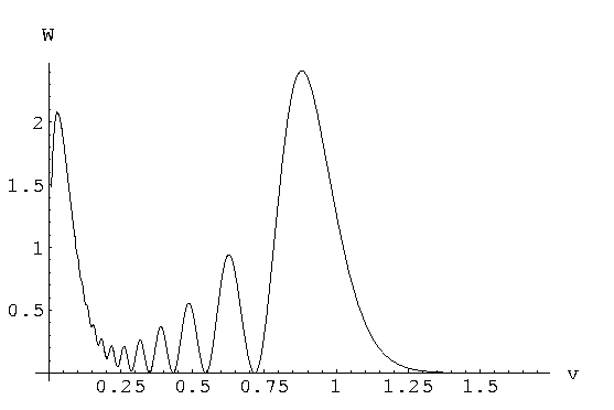
Figure 1: Spectrum of radiation for $\sigma$-component at an angle $\chi=0$. The initial phase is $\delta=0$

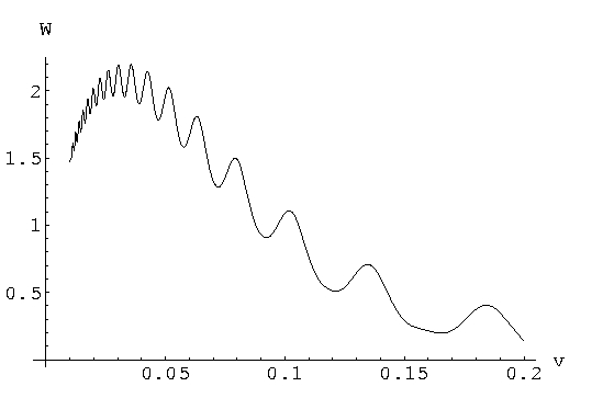
Figure 2: Spectrum of radiation for $\sigma$-component at an angle $\chi=0$. The initial phase is $\delta=\pi/6$.

Figures 1 and 2 show the dependence of spectrum of radiation on parameters $k$, $\delta$ and $N$. The low-frequency part exhibits the curvature radiation while the high-frequency part represents the undulator radiation. We see that the undulator radiation is emitted at basic harmonic $\nu\approx 1$, and the curvature radiation is situated around frequency $\omega_{cr}\approx\omega_{ur}/N$, i.e. $\nu\approx 0.05$. Figure 2 demonstrates the influence of initial phase upon the shape of the spectrum. The small oscillations of the spectrum curve is highly dependent on the value of the initial phase $\delta$.

The dependence on the pitch-angle $\alpha$ is included in the undulator parameter $k$. Formula (11) shows that the undulator part of radiation increases with increasing $\alpha$.

References

[1] J.L.Zhang and K.S.Cheng, Phys. Lett.A 208,
47 (1995).
[2] K.S.Cheng and J.L.Zhang, ApJ 463, 271 (1996).
[3] L.Landau and E.Lifshitz, The Classical Theory of
Fields (Pergamon, London), 1962.
[4] M.M.Nikitin and V.Ya.Epp, Undulator Radiation
(Energoatomizdat, Moscow), 1988.
[5]Synchrotron Radiation Theory and Its
Development. Ed. by V.A. Bordovitsyn. (World Scientific, Singapore),
1999.