Microphysics in the gamma ray burst central engine

Abstract

We calculate the structure and evolution of a gamma ray burst central engine where an accreting torus has formed around the newly born black hole. We study the general relativistic, MHD models and we self-consistently incorporate the nuclear equation of state. The latter accounts for the degeneracy of relativistic electrons, protons, and neutrons, and is used in the dynamical simulation, instead of a standard polytropic $\gamma$-law. The EOS provides the conditions for the nuclear pressure in the function of density and temperature, which evolve with time according to the conservative MHD scheme. We analyze the structure of the torus and outflowing winds, and compute the neutrino flux emitted through the nuclear reactions balance in the dense and hot matter. We also estimate the rate of transfer of the black hole rotational energy to the bipolar jets. Finally, we elaborate on the nucleosynthesis of heavy elements in the accretion flow and the wind, through computations of the thermonuclear reaction network. We discuss the possible signatures of the radioactive elements decay in the accretion flow. We suggest that further detailed modeling of the accretion flow in GRB engine, together with its microphysics, may be a valuable tool to constrain the black hole mass and spin. It can be complementary to the gravitational wave analysis, if the waves are detected with an electromagnetic counterpart.

1. Introduction

Gamma Ray Bursts (GRB), are extremely energetic transient events, visible from the most distant parts of the Universe (Piran , 2004; Kumar & Zhang , 2015). When a newly born black hole forms, either via the core collapse supernova, or after the merger of two compact stars, a large amount of matter is accreted onto it within the timescale between tens of milliseconds, to thousands of seconds, with hyper-Eddington rates (Woosley , 1993; Paczynski , 1998). In such conditions, the nuclear reactions inside the plasma lead to creation of neutrinos, mainly via the electron-positron capture on nucleons, which acts in the so-called NDAF models (Narayan et al. , 2000; Lei et al. , 2009; Cao et al. , 2014). The annihilation of neutrino-antineutrino pairs is a source of power to the relativistic jets launched along the axis of the disk-black hole system. This can be comparable to the power extracted on the cost of the black hole spin, with the disk mediated by the magnetic fields. Both neutrinos and magnetic fields in the accreting matter can drive the wind outflow from the disk surface, and act as a collimation mechanism for the relativistic jets (see, e.g., Lee & Ramirez-Ruiz 2007 and references therein). The latter, are then the sites of the high-energy radiation produced at large distances from the engine, on the cost of the magnetic reconnection and conversion of the jet electromagnetic energy flux into heat (e.g., Bromberg & Tchekhovskoy 2016).

Numerical computations of the structure and evolution of the accretion flow in the gamma ray bursts engine begun with steady-state, and time-dependent models, which were axially and vertically averaged, and based on the classical prescription for viscosity with the so-called $\alpha$-parameter (Popham et al. , 1999; Di Matteo et al. , 2002; Kohri & Mineshige , 2002; Kohri et al. , 2005; Reynoso et al. , 2006; Chen & Beloborodov , 2007; Janiuk et al. , 2004, 2007; Janiuk & Yuan , 2010). More recently, these accretion flows are being described by fully relativistic, MHD computations (Shibata et al. , 2007; Nagataki , 2009; Barkov & Komissarov , 2010; Barkov & Baushev , 2011; Rezzolla et al. , 2011; Janiuk et al. , 2013; Kiuchi et al. , 2015).

In the outer parts of the disc, the heavy elements can be formed, and then the isotopes are prone to the radioactive decay (Fujimoto et al. , 2004). This may in the future bring observable effects on the measured hard X-ray spectra of GRBs (Janiuk , 2014) as well as the additional peaks in the blue and infrared bands a few days after the prompt GRB emission (Martin et al. , 2015). In addition, the gamma ray bursts contribute in this way to the galactic chemical evolution (Surman et al. , 2014). The physical conditions in this engine, its density, temperature, and electron fraction, depend on the global parameters of the flow, such as the amount of matter and accretion rate, black hole mass and its spin, and the magnetic field. These conditions in turn will affect the total abundances of heavier elements synthesized within the flow. Therefore, a possible detection of the signatures of the radioactive decay of these species, and quantitative modeling of nucleosynthesis together with the central engine structure and evolution, and the jets gamma ray fluence, could give a constraint on the black hole parameters. These, in turn, can now be independently estimated, if the black hole is born via a merger event, detectable in the gravitational wave interferometer.

In this work, we study the central engine of a gamma ray burst, which is composed of a stellar mass, rotating black hole and accreting torus that has formed from the remnant matter at the base of the GRB jet. We compute the time-dependent, two dimensional model of the rotationally supported, magnetized disc, rapidly accreting onto the center. The simulation is based on the HARM (High Accuracy Magnetohydrodynamics) scheme, which works on the stationary metric around black hole. The code integrates the total energy equation and updates the set of ’conserved’ variables, i.e. comoving density, energy-momentum, and magnetic field (Gammie et al. , 2003).

The basic version of the HARM scheme was designed to model the accretion flows in the centers of galaxies, where the gas equation of state is with a good accuracy given by that of an ideal gas, and can be described using an adiabatic relation (e.g., Moscibrodzka & Falcke 2013). In our current dynamical model, we use the non-ideal equation of state, computed on the basis of the $\beta$-equilibrium (Janiuk et al. , 2007). We allow for the partial degeneracy of relativistic nucleons, electrons and positrons in the accreting plasma, and we compute the neutrino cooling rate due to the weak interaction processes, electron-positron pair anihillation, as well as bremsstrahlung and plasmon decay. Here, we for the first time incorporate this detailed microphysics into the heart of the GR MHD scheme. The neutrino cooling was computed already from the nuclear reaction balance in the context of gamma ray bursts in our previous work (Janiuk et al. , 2013). However, in that work, still the simple, adiabatic relation for the pressure ($p=(\gamma-1)u$, with $\gamma=4/3$) was used, and only the internal energy of the gas was updated during the simulation. In the current model, we mainly address the question of microphysics in the accretion flow, and we are now also able to self-consistently estimate the efficiency of the disk neutrino cooling. We check if it is capable of powering the relativistic jets in the gamma ray bursts, now in the case of a rather weak magnetic field. We also check the effect of the rotation speed of the black hole. In addition, we analyze the structure, velocity and amount of mass loss through the uncollimated winds launched from the accretion disc. Finally, we examine the resulting nucleosynthesis in the body of the disk, which can occur already at small distances from the black hole, as well as in the winds, and we show that the accretion flow can be the site of significant production of heavy element.

The article is organized as follows. In § 2, we describe our MHD model of the GRB central engine. In § 3, we present the results, describing the structure of the torus and the effects of adopted microphysics treatment. We also compute the power transferred to the GRB jets via the neutrino anihillation and compare it to the energy extracted by the magnetic fields dragged through the BH horizon. In § 4 we describe the process of heavy elements formation in the outskirts of the torus in the GRB engine. We present the resulting abundances of elements computed under the assumption of nuclear statistical equilibrium. Finally, we compare our results with the previous simulations. We discuss the results in § 5.

2. Model of the hyperaccreting disk

The model computations are based on the axisymmetric, general relativistic MHD code HARM-2D, described by Gammie et al. (2003) and Noble et al. (2006). It uses a conservative, shock-capturing scheme, and provides solver for the continuity and energy-momentum conservation equations, assuming a force-free approximation. Here we use our own version of this code, which we supplemented with the numerical routines to compute the equation of state and rate of cooling by neutrinos.

2.1. Equation of state and neutrino cooling

The neutrino cooling processes adopted in our computations are the reactions of electron and positron capture on nucleons, the electron-positron pair anihillation, nucleon bremsstrahlung and plasmon decay. The capture reactions are:

$$p+e^{-}\to n+\nu_{\rm e}$$

$$p+\bar{\nu}_{\rm e}\to n+e^{+}$$

$$p+e^{-}+\bar{\nu}_{e}\to n$$

$$n+e^{+}\to p+\bar{\nu}_{\rm e}$$

$$n\to p+e^{-}+\bar{\nu}_{\rm e}$$

$$n+\nu_{\rm e}\to p+e^{-},$$ (1)

and their reaction rates are given by appropriate integrals (Reddy et al. , 1998; Janiuk et al. , 2007). In addition, the neutrinos are produced due to the electron-positron pair anihillation, bremsstrahlung, plasmon decay, in the following reactions:

$$e^{-}+e^{+}\to\nu_{\rm i}+\bar{\nu}_{\rm i}\\$$

$$n+n\to n+n+\nu_{\rm i}+\bar{\nu}_{\rm i}\\$$

$$\tilde{\gamma}\to\nu_{\rm e}+\bar{\nu}_{\rm e}.\\$$

We calculate their rates numerically, with proper integrals over the distribution function of relativistic, partially degenerate species. Finally, the total neutrino cooling rate is given by the two-stream approximation (Di Matteo et al. , 2002), and it includes the scattering and absorptive optical depths for neutrinos of the three flavors:

$$Q^{-}_{\nu}={{7\over 8}\sigma T^{4}\over{3\over 4}}\sum_{i=e,\mu,\tau}{1\over{\tau_{\rm a,\nu_{i}}+\tau_{\rm s}\over 2}+{1\over\sqrt{3}}+{1\over 3\tau_{\rm a,\nu_{i}}}}\times{1\over H}\;,$$ (2)

and is expressed in the units of erg s^-1cm^-3.

The structure of a magnetized accreting torus in which the above reactions take place and the gas looses energy via neutrino cooling, was investigated in our previous paper (Janiuk et al. , 2013). In that work, however, the neutrino cooling rate was used to update in every time step only the internal energy in the plasma, and the pressure was still approximately computed from the adiabatic relation, $p=(\gamma-1)u$, with constant $\gamma=4/3$, which simplifies a lot the GR MHD scheme.

The leptons and baryons are relativistic in the GRB engine, and may have an arbitrary degeneracy level, so we compute the gas pressure using the Fermi-Dirac distribution of the species. Also, neutrinos may contribute to the pressure due to the fact that they are scattered and absorbed, similarly to the photons and (rather negligibly small in the GRB case) radiation pressure component. In the total pressure, we include now the contributions from the free nucleons, pairs, radiation, trapped neutrinos, and also from the Helium nuclei.

$$P_{\rm gas}=P_{\rm nucl}+P_{\rm He}+P_{\rm rad}+P_{\nu}$$ (3)

where $P_{\rm nucl}$ includes free neutrons, protons, and the electron-positrons:

$$P_{\rm nucl}=P_{\rm e-}+P_{\rm e+}+P_{\rm n}+P_{\rm p}$$ (4)

with

$$P_{\rm i}={2\sqrt{2}\over 3\pi^{2}}{(m_{i}c^{2})^{4}\over(\hbar c)^{3}}\beta_{i}^{5/2}\left[F_{3/2}(\eta_{\rm i},\beta_{\rm i})+{1\over 2}\beta_{\rm i}F_{5/2}(\eta_{\rm i},\beta_{\rm i})\right].$$ (5)

Here, $F_{\rm k}$ are the Fermi-Dirac integrals of the order $k$, and $\eta_{\rm e}$, $\eta_{\rm p}$ and $\eta_{\rm n}$ are the reduced chemical potentials, $\eta_{i}=\mu_{i}/kT$ is the degeneracy parameter, where $\mu_{i}$ is the standard chemical potential. Reduced chemical potential of positrons is $\eta_{\rm e+}=-\eta_{\rm e}-2/\beta_{\rm e}$. Relativity parameters are defined as $\beta_{\rm i}=kT/m_{\rm i}c^{2}$. The total pressure is computed numerically by solving the balance of nuclear reactions (Yuan , 2005; Janiuk & Yuan , 2010).

2.2. Initial conditions and dynamical model

The numerically computed nuclear EOS is incorporated now into the MHD scheme, with the pressure determined as a function of density and temperature. The MHD scheme solves for the inversion between the so called ’primitive’ and ’conserved’ variables at every time-step (see e.g., Noble et al. 2006). The code HARM-2D provides solver for continuity and energy-momentum conservation equations:

$$(\rho u^{\mu})_{;\mu}=0$$ (6)

and

$${T^{\mu}}_{\nu;\mu}=0,$$ (7)

where:

$$T^{\mu\nu}=T^{\mu\nu}_{\rm gas}+T^{\mu\nu}_{\rm EM}$$

$$T^{\mu\nu}_{\rm gas}=\rho hu^{\mu}u^{\nu}+pg^{\mu\nu}=(\rho+u+p)u^{\mu}u^{\nu}+pg^{\mu\nu}$$

$$T^{\mu\nu}_{\rm EM}=b^{2}u^{\mu}u^{\nu}+\frac{1}{2}b^{2}g^{\mu\nu}-b^{\mu}b^{\nu};~{}~{}b^{\mu}=u_{\nu}{{}^{{}^{*}}\!\!F}^{\mu\nu}$$

and $u^{\mu}$ is the four-velocity of gas, $u$ is the internal energy density, $b^{\mu}=\frac{1}{2}\varepsilon^{\mu\nu\rho\sigma}u_{\nu}F_{\rho\sigma}$ is the magnetic four-vector, and $F$ is the electromagnetic stress tensor. Assuming the force-free approximation, we have $E_{\nu}=u_{\mu}F^{\mu\nu}=0$.

The conservative numerical scheme which is used in this code, in general solves ${\partial}_{t}{\bf U}({\bf P})=-{\partial}_{i}{\bf F}^{i}({\bf P})+\mathbf{S}({\bf P})$ where ${\bf U}$ is a vector of “conserved” variables (momentum, energy density, number density, taken in the coordinate frame), ${\bf P}$ is a vector of ’primitive’ variables (rest mass density, internal energy), ${\bf F}^{i}$ are the fluxes, and $\mathbf{S}$ is a vector of source terms.

In contrast to the non-relativistic MHD, where ${\bf P}\rightarrow{\bf U}$ and ${\bf U}\rightarrow{\bf P}$ have a closed-form solution, in relativistic MHD, ${\bf U}({\bf P})$ is a complicated, nonlinear relation. Inversion ${\bf P}({\bf U})$ is calculated therefore, in every time step, numerically. The inverse transformation requires to solve a set of 5 non-linear equations, which is done by a multi-dimensional Newton-Raphson routine. The procedure is simple, if the pressure is given by an adiabatic relation with density. However, for a general equation of state, one must compute also $dp/dw$, $dp/dv^{2}$, and $p(W,v^{2},D)$ (here we have enthalpy, $w=p+u+\rho$; $W=\gamma^{2}w$; $D=\sqrt{-g}\rho u^{t}$). In our scheme, we have tabulated pressure and internal energy as a function of density and temperature, $(p,u)(\rho,T)$, and we interpolate over this table. In addition, density and temperature in the flow give us a unique determination of the neutrino cooling rate. The Jacobian $\partial{\bf U}/\partial{\bf P}$ is computed numerically, and the conserved variables are evolved in time. To speed up the computations, our version of this code was parallelized using the MPI technique, for the hydro-evolution, and we also implemented the shared memory hyper-threading for the EOS-table interpolation.

The simulations are conducted in 2D, on the spherical grid with the resolution of 256x256 cells in the $r$ and $\theta$ directions, and typically run up to t=2000-3000 M in dimensionless units (c=G=1). The grid is spaced logarithmically in radius and concentrated towards the equatorial plane, defined as in Gammie et al. (2003).

The initial conditions for the accretion flow are given by the equilibrium torus solution, defined as in Fishbone & Moncrief (1976) and Abramowicz et al. (1978). The parameters of the model are the black hole mass and its spin. The torus mass is defined by the radius of the pressure maximum, and it is also supplemented with the density scaling, which is necessary to compute the pressure and temperature in the torus in physical units. The model is seeded by the initial magnetic field. The magnetic field in our current computations is adopted to have a standard, poloidal configuration given with the $\phi$-component of its vector potential scaling with the density, $A_{\phi}=(\rho/\rho_{max})$, and is weakly magnetized, with an initial $\beta=P_{\rm gas}/P_{\rm mag}=50$ (see e.g., McKinney, Tchekhovskoy & Blandford (2012) for the discussion of various other field configurations).

3. Structure of the flow

3.1. Accreting torus and wind outflow

Our choice of the setup and parameters is meant to reproduce the properties of the typical engine of a short gamma ray burts, however, to some extent, the computations are scalable with the black hole and accretion disk mass. Nevertheless, in the discussed models, we assume no matter supply through the outer boundary to the computational domain, which would result, e.g., from a fallback of the collapsar’s envelope in case of long GRBs. We choose in this Section a fiducial value of $M_{\rm BH}=3M_{\odot}$, as an order of magnitude adequate to be a result of a compact binary merger. The torus mass is taken here to be of about 0.1 $M_{\odot}$, so that the accretion rate in physical units is on the order of 1 Solar mass per second (Kluzniak & Lee , 1998). The initial conditions introduced from the pressure equilibrium solution are relaxed after about $1000M$ (we express the time in dimensionless units, with $G=c=1$, so that the physical unit of time in seconds will be $t_{\rm unit}=GM/c^{3}$), and then the torus evolves to the form the dynamically driven, geometrically thin flow, which is accreting through the black hole horizon. In the example Figure 1, we plot the radial profiles of the torus thickness for the cooled torus, at four time snapshots. The initial condition represents the equilibrium torus (a ’doughnut’) and this profile spreads with time into larger radii. The torus thickness is computed from the pressure scale-height, as follows

$$H={1\over\Omega}c\sqrt{P\over\rho c^{2}+e},$$ (9)

where $\Omega={c^{3}\over GM}{1\over(a+r^{3/2})}$ is the Keplerian frequency and the sound speed is approximately given by its relativistic form (see Ibanez et al. (2015)). The thickness of the torus is about $H/r\sim 0.2$. The exact value depends on the black hole spin, both in the initial equilibrium and time-dependent solution. The maximum thickness of the torus, defined above, reaches the values from 7 to 9 $r_{\rm g}$ in the initial model, for the spins from 0.6, to 0.98. The maximum thickness at the time $t=2000M$ increases to about 10-14 $r_{\rm g}$, for this range of spins. Also, as the Figure 1 shows, it is shifted to the outer boundary, while the torus no longer keeps its equilibrium ’doughnut’ shape.

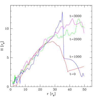
Figure 1.— Thickness of the torus in the function of radius, at four different time snapshots during the simulation, t=0, 1000, 2000, and 3000 M, as labelled in the plot and marked by different colors. The model includes numerical EOS and neutrino cooling. Parameters of the model are $M_{\rm BH}=3M_{\odot}$, $M_{\rm torus}\approx 0.1M_{\odot}$. Black hole spin is $a=0.9$.

In Figure 2 we plot the accretion rate through the black hole horizon in the function of time. The mean rate of accretion is about 0.3-0.4 $M_{\odot}$ s^-1, for the black hole mass of 3 $M_{\odot}$, depending slightly on the black hole spin (see Table 1). The instantaneous peaks which appear in the states of a highly variable accretion rate, reach the values up to several Solar mass per second. These flares disappear as the initial condition is evolved, and then the accretion rate varies only by a few per cent. The flares in the local accretion rate do not necessarily correspond to the observable luminosity flares. In fact, the neutrino luminosity which we derive by integrating the emissivity over the whole simulation volume, has a smooth dependence on time. In case if the high accretion rate through the black hole horizon affects somehow the jet production, this rapid variability might have observable consequences. The direct predictions however are not possible with the current model.

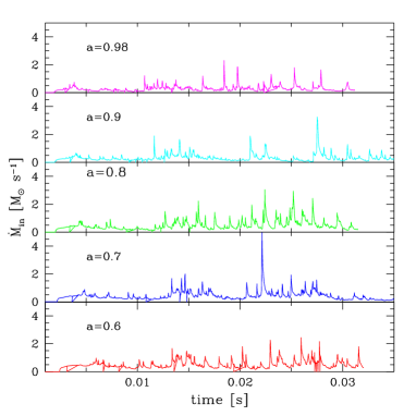
Figure 2.— Accretion rate as a function of time, in the models with neutrino cooling. The models were calculated for a range of black hole spin parameters: a=0.6, 0.7, 0.8, 0.9, and 0.98, with red, blue, green, yellow, and magenta lines, respectively. The black hole mass is equal to $3M_{\odot}$, and the initial disk mass is about $0.1M_{\odot}$

In Figure 3 we show the two-dimensional maps of the torus structure, in the $r-\theta$ plane, obtained from the calculations with the black hole mass of 3 $M_{\odot}$ and spin of $a=0.6$. The snapshots from our simulation were taken at time $t=2000M$, which for the adopted black hole mass is equivalent to about 0.03 s. The maps present the rest mass density $\rho$, gas temperature $T$, and magnetic pressure to gas pressure ratio $\beta$, over-plotted with magnetic field lines. We also show the distribution of the neutrino emissivities within the flow, as computed from the equation of state of matter with these profiles of temperature and density. The last panel to the right in Figure 3, presents the velocity field in the flow. The arrows (with normalized length) show the direction of velocity, while the color map presents the ratio of the flow velocity to the speed of light, $v/c=\sqrt{g^{\mu\nu}u^{\mu}u^{\nu}}$. The turbulent velocity field in the torus is changing into a uniform outflow which is launched above the torus surface at high latitudes.

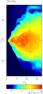
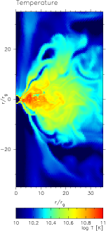
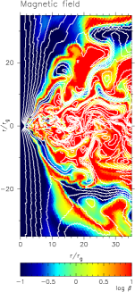
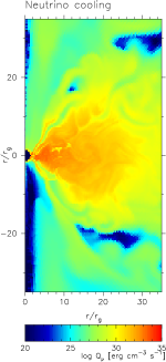
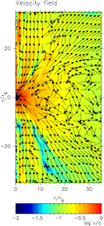
Figure 3.— Structure of accretion disk at the end of the simulation. The model accounts for the neutrino cooling and nuclear EOS. The maps show: (i) density, (ii) temperature of the plasma, (iii) ratio of gas to magnetic pressure, with field lines topology, (iv) neutrino emissivity $Q_{\nu}$, and (v) velocity field (from left to right). The snapshots are taken at time t=2000 M, which is equivalent to $t\approx 0.03$ s. Parameters of the model: black hole mass $M_{\rm BH}=3M_{\odot}$, torus mass $M_{\rm t}=0.1M_{\odot}$, and BH spin $a=0.6$.

The disk winds are sweeping the gas out from the system, both in the equatorial plane and at higher latitudes. We identified the regions of the wind in the computation domain by defining three conditions that must be satisfied simultaneously. In order to distinguish the wind from the torus main body, and from the magnetized jets: (i) the radial velocity of the plasma is positive (ii) the density is smaller than $10^{9}$ g cm³ and (iii) the gas pressure is dominant, $\beta>1.0$. The winds are located approximately at radii above 10 $R_{\rm g}$ and latitudes between about $30^{\circ}-60^{\circ}$ and $120^{\circ}-150^{\circ}$. The velocity in the wind is typically $v/c\sim 0.06-0.5$, and its maximum value is only slightly depending on the black hole spin. The density in the wind, by definition, is below $10^{9}$ g sm^-3, but may drop down to $10^{5}$ g cm^-3. The temperature of the wind in the neutrino cooled models is in the range of $6\times 10^{9}-5.7\times 10^{10}$ K. Such high temperatures, above the threshold for electron-positron pair production, $T=m_{\rm e}c^{2}\approx 5\times 10^{9}$ K, are the key condition for neutrino emission processes. The neutrino cooling is then efficient, as it only weakly depends on density. In the clumps with $\rho>\sim 10^{8}$ g cm^-3, the nuclear processes lead to neutrino production, while the optical depths for their absorption are very small.

The effect of the wind is the mass loss from the system. We estimated quantitatively the evolution of the mass during the simulation. The total mass removed from the torus during the simulation, calculated by integrating the density over the total volume, differs from the total mass accreted onto the black hole (i.e. the time integrated mass accretion rate through the inner boundary, subtracted from the initial mass). This may depend on the black hole spin. For the model with $a=0.6$, the simulation was ended when the total mass in the volume dropped below $0.089M_{\odot}$. The starting mass at $t=0$, was equal to $0.11M_{\odot}$. During the simulation, about 0.014 Solar masses was accreted onto the black hole (which makes 20% of the initial mass), and the rest, about 6%, was lost from the computation domain in the outflows. For larger black hole spins, the fraction of mass lost through wind can reach about 10%. The values for all the models are collected in Table 1.

The hot, magnetized, transient polar jets appear as well, and they form on both sides of the black hole, as can be seen in the maps in Figs. 3. They are present in a narrow region along the polar axis, where the open magnetic field lines have formed. Velocity field is directed there outwards, and the gas is expelled from the black hole region with the velocity that is nearly at the speed of light.

3.2. Neutrino luminosity and Blandford-Znajek energy extraction

The total neutrino luminosity in the function of time is shown in Figure 4, where we present the results for the black hole mass of 3 $M_{\odot}$ and torus mass of $\approx 0.1M_{\odot}$. The luminosities are plotted for a range of black hole spins: $a=0.6,0.7,0.8,0.9$, and 0.98. Initially, the total integrated neutrino luminosity is in the range of $6\times 10^{52}$-$2\times 10^{53}$ erg s^-1, and temporarily drops, when the matter starts accreting. As the initial state is evolved, the luminosity grows to over $10^{53}$ erg s^-1 and at time $t=0.03$ s reaches roughly a constant level, which is scaling with the black hole spin. The exact values of $L_{\nu}$ at the end of the simulation are given in Table 1.

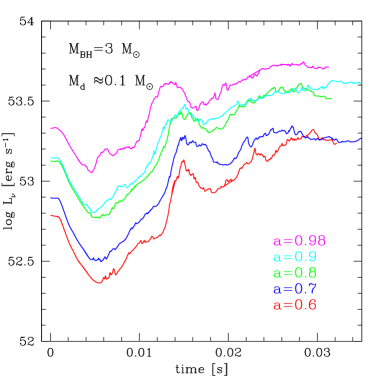
Figure 4.— Total neutrino luminosity as a function of time. The black hole mass is $M_{\rm BH}=3M_{\odot}$ and torus initial mass is $M_{\rm d}\sim 0.1M_{\odot}$. The models were calculated for a range of black hole spin parameters, $a=0.98,0.9,0.8,0.7$, and 0.6, as marked with magenta, yellow, green, blue, and red lines, respectively.

The neutrinos are emitted from the torus as well as from the hot, rarefied wind. The wind contribution to the total luminosity is of about 10-11% for all the models. The luminosity of the densest parts of the torus, estimated by weighing the total emissivity by the plasma density, is only on the order of $10^{48}-10^{49}$ erg s^-1. This is because the total opacity for neutrino absorption and scattering in this regions reaches $\tau\sim 1-5$, and the neutrinos are trapped in the dense plasma.

The power and luminosity available through the Blandford-Znajek process (Blandford & Znajek , 1977) is calculated from the electromagnetic stress tensor, given by

$$T^{\mu\nu}_{\rm EM}=b^{2}u^{\mu}u^{\nu}+\frac{b^{2}}{2}g^{\mu\nu}-b^{\mu}b^{\nu},$$ (10)

where $b^{\mu}$ is the magnetic four-vector, with $b^{t}=g_{i\mu}B^{i}u^{\mu}$ and $b^{i}=(B^{i}+u^{i}b^{t})/u^{t}$ and $u^{\mu}$ is the four-velocity. We compute the radial electromagnetic flux through the horizon as in McKinney & Gammie (2004):

$$\dot{E}=2\pi\int_{0}^{\pi}d\theta\sqrt{-g}F_{\rm EM},$$ (11)

where $F_{\rm EM}=-T^{r}_{t}$ and $g$ is the metric determinant. We consider only the flux, which is dragged inwards through the black hole horizon, and we also check the magnetization of the plasma there, $\beta(r_{\rm in})=B^{2}/\rho(r_{\rm in})$, where $\rho$ is the rest mass density of the gas. We impose a condition of $\beta(r_{\rm in})\geq 1.0$, otherwise the Blandford-Znajek power is set to be zero. This is because we want to focus on the energy extracted to the magnetically dominated polar jets. The outward directed energy flux can be in fact present also close to the equator, at moderate altitudes, where the matter is dense and weakly magnetized. The contribution of this equatorial flux to the total power is only about 5-15%, if the black hole spin is $a\geq 0.9$, however it can be dominant for the models with small black hole spins, when the magnetized jets are not formed. In some runs, the dense and transient clumps of matter temporarily appear in the polar regions, so that the jet is contaminated and its BZ luminosity temporarily vanishes (see Figure 5). Our condition is therefore numerically equivalent to the method of jet ’cleaning’, used by other authors (see e.g. Tchekhovskoy & Bromberg 2016).

The resulting BZ luminosities in the function of time for the range of black hole spin values in different models are presented in Figure 5. As the Figure shows, the continuous power supply to the jet of above $10^{52}$ erg s^-1 is available only for the highly spinning black holes. If the spin is moderate, $a=0.6-0.8$, then the power $L_{\rm BZ}\approx 10^{51}$ erg s^-1 is injected. Episodically, the power drops to zero, when there is no magnetization on the black hole horizon. Therefore, the power injection can be separated by the intervals of the ’BZ-quiescence’, which can be longer if the black hole spin is small.

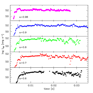
Figure 5.— Power extracted from the black hole rotation through Blandford-Znajek process, and resulting luminosity as a function of time. The model includes numerical EOS and neutrino cooling. Parameters of the model are $M_{\rm BH}=3M_{\odot}$, torus mass $M_{\rm t}\approx 0.1M_{\odot}$. The black hole spin values are marked in the panels, and range from a=0.6, to a= 0.98, from bottom to top panels

The exact values of the BZ-luminosity at the end of the simulations are given in Table 1.

Table 1Summary of the models. Black hole mass is $3M_{\odot}$. The mass of the torus is given in $M_{\odot}$, accretion rate in $M_{\odot}$s^-1, the time is in seconds, and luminosity in erg s^-1.

Model	$a$	$R_{\rm max}$	$t_{\rm e}$	$M_{\rm t}(t_{0})$	$M_{\rm t}(t_{\rm e})$	$<\dot{M}>$	$\dot{M}(t_{\rm e})$	$\Delta M_{\rm w}$	$L^{\rm tot}_{\nu}(t_{\rm e})$	$L_{\rm BZ}(t_{\rm e})$
sAc	0.6	11.8	0.028	0.11	0.082	0.49	0.30	0.012	$1.69\times 10^{53}$	$1.83\times 10^{50}$
sBc	0.7	11.0	0.029	0.10	0.072	0.45	0.29	0.014	$1.67\times 10^{53}$	$2.99\times 10^{51}$
sCc	0.8	10.5	0.029	0.12	0.086	0.46	0.35	0.018	$3.40\times 10^{53}$	$5.45\times 10^{50}$
sDc	0.9	9.75	0.028	0.10	0.075	0.31	0.22	0.015	$3.62\times 10^{53}$	$2.59\times 10^{52}$
sEc	0.98	9.1	0.028	0.11	0.083	0.28	0.20	0.017	$5.25\times 10^{53}$	$6.6\times 10^{51}$
sAnc	0.6	11.8	0.032	0.11	0.090	0.46	0.31	0.005	–	$1.0\times 10^{49}$
sBnc	0.7	11.0	0.031	0.10	0.084	0.37	0.18	0.004	–	$2.8\times 10^{50}$
sCnc	0.8	10.5	0.044	0.12	0.108	0.24	0.04	0.004	–	$4.43\times 10^{50}$
sDnc	0.9	9.75	0.041	0.10	0.089	0.23	0.177	0.003	–	$2.52\times 10^{51}$
sEnc	0.98	9.1	0.035	0.11	0.097	0.18	0.109	0.007	–	$7.62\times 10^{51}$

3.3. Comparison to the models without neutrino cooling

To quantify the effect of microphysics, equation of state, and the neutrino cooling in 2D MHD simulations, we ran a set of test models with no cooling and adiabatic equation of state with $\gamma=4/3$, as in the standard HARM models. The model parameters and initial conditions were otherwise the same.

In Figure 6 we plot the rate of matter accretion through the inner boundary, as a function of time for a set of models with various black hole spins. The average accretion rate onto black hole is slightly lower in the adiabatic models than in the cooled models, for the same model parameters. The initial conditions are evolved slower in the adiabatic case, and the flaring peaks in the accretion rate appear for a longer time. The highest peak in this set of models appeared for $a=0.6$, and not for $a=0.7$, which was the case in the neutrino cooled torus. The quasi-stationary, almost constant accretion rate appears after $t\approx 0.04$, and the mean value of the accretion rate is on the same order as in neutrino cooled models, but somewhat lower (see Table 1 for exact values).

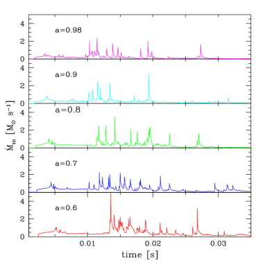
Figure 6.— Accretion rate as a function of time, in the models without neutrino cooling, with polytropic EOS adopted with $\gamma=4/3$. The values of black hole mass, spin, and disk mass are denoted in the figure.

In the adiabatic models, the neutrino luminosity is set to zero, by definition. The only source of the energy extraction and power supply to the jets is therefore the rotation of the black hole and magnetic flux. In Figure 7 we show the Blandford-Znajek luminosity in the function of time for this set of models, with various spins. We note that for the highest black hole spins, $a=0.9-0.98$, the BZ luminosity is equally large as for the neutrino cooled tori, and it is almost constant with time. However, for the models with black hole spins of $a=0.6-0.8$, the BZ power drops later in the evolution, and after $t\approx 0.02$ it is smaller than about $10^{50}$ erg s^-1. In other words, the energy extraction from the moderately rotating black hole by magnetic fields is less efficient, when the torus is not cooled by neutrinos.

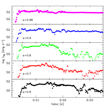
Figure 7.— Power extracted from the black hole rotation through Blandford-Znajek process, and resulting luminosity as a function of time. The model is based o the adiabatic EOS, with $\gamma=4/3$, and no neutrino cooling. Parameters of the model are $M_{\rm BH}=3M_{\odot}$, torus mass $M_{\rm t}\approx 0.1M_{\odot}$. The black hole spin values are marked in the panels, and range from a=0.6, to a= 0.98, from bottom to top panels

The maps of the density, temperature, velocity and magnetic field in the exemplary model with $a=0.6$, are shown in Figure 8. The density of the disk in the models without cooling is larger in the equatorial plane, while the disk seems to be compact (i.e., denser and geometrically thinner) close to the black hole. Due to the lack of neutrino cooling, it is also hotter than that presented in the Figure 3. The highest temperatures are achieved in the regions below 10 $r_{\rm g}$ in the disk, and also in the outflows (winds). Open magnetic field lines are formed, even for the small black hole spin, but in general the flow is less magnetized and the gas pressure is large both in the disk and in the winds. The velocity field map shows the cooler, low density outflowing clumps, confined along the vertical axis.

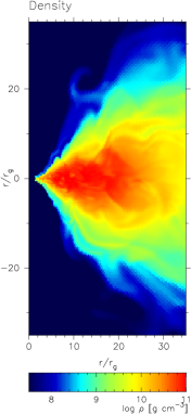
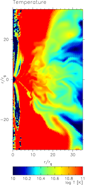
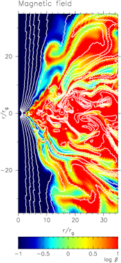
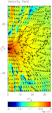
Figure 8.— Model without neutrino cooling and with adiabatic equation of state. The parameters are: $a=0.6$, $M_{\rm BH}=3M_{\odot}$, $\beta_{\rm init}=50$, torus mass $M_{\rm t}\approx 0.1M_{\odot}$. The maps, from left to right, show the distribution of density, temperature, ratio of gas to magnetic pressure with field lines topology, and velocity field. The snapshots are taken at $t=2000M$, which is equivalent to $t\approx 0.03$ s of the dynamical simulation.

The thickness of the torus, measured by the scale height given by Eq. 9 is shown in the Figure 9. In the adiabatic models, the disk is thicker geometrically, and at outer regions the ratio $H/r$ saturates at the value of about 0.3-0.4. The mass loss rate is smaller than in the case of neutrino cooled tori, and typically only 1-3% of the torus mass is lost in the wind during the simulation. For the model with black hole spin close to maximal, $a=0.98$, the total mass loss in the wind outflow is completely negligible, within our numerical accuracy.

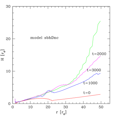
Figure 9.— Thickness of the torus as a function of radius, in the models without neutrino cooling, with polytropic EOS adopted with $\gamma=4/3$. The model is with the black hole spin $a=0.9$.

4. Nucleosynthesis of heavy elements

In the astrophysical plasma, thermonuclear fusion occurs due to the capture and release of particles ($n$, $p$, $\alpha$, $\gamma$). Reaction sequence produces further isotopes, and the set of non-linear differential equations is solved by the Euler method (Meyer , 1994; Wallerstein et al. , 1999). The nuclear reactions may proceed with 1 (decays, electron-positron capture, photodissociacion), 2 (encounters), or 3 (triple alpha reactions) nuclei. Abundances of the isotopes are calculated under the assumption of nucleon number and charge conservation for a given density, temperature and electron fraction ($T\leq 1MeV$). Integrated cross-sections depending on temperature $kT$ are determined with the Maxwell-Boltzmann or Planck statistics, and the background screening and degeneracy of nucleons must be taken into account.

We use the thermonuclear reaction network code http://webnucleo.org, and determine the relative abundances of heavy elements in the accreting torus. Given the density, temperature, and electron fraction, the nuceq library is used, and we compute the nuclear statistical equilibria established for the thermonuclear fusion reactions, taking the reaction rates available on JINA reaclib online database (Hix & Meyer , 2006; Seitenzahl et al. , 2008). This network is appropriate for temperatures below $1MeV$, which is the case at the outer radii of accretion disks in GRB engines. The mass fraction of the isotopes is solved for converged profiles of density, temperature and electron fraction in the disk, defined as:

$$Y_{\rm e}=\frac{n_{\rm e^{-}}-n_{e^{+}}}{n_{\rm b}}.$$ (12)

We use here a standard, publicly available software, and a more detailed description of our procedure can be found in Janiuk (2014).

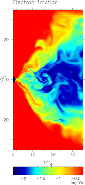
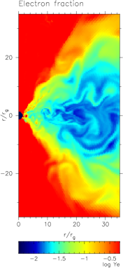
Figure 10.— Electron fraction distribution. The snapshots are taken at $t=2000M$. Models shown in the left and right panels are $sAc$ and $sDc$, as labeled in the Table 1, respectively, and differ with the black hole spin.

In Figure 10 we plot the electron fraction in the 2-D maps of the accretion flow. The parameters of this simulation were: the black hole of mass equal to $3M_{\odot}$, torus mass of about $0.11M_{\odot}$, and the black hole spins of 0.6 and 0.9, as shown in the left and right panels, respectively. Distributions are plotted for the evolved simulation, at $t=2000M$.

In Figure 11 we show the abundances of heavy elements, for these two models, which are produced in the torus and wind. The numbers are integrated up to the distance of $1000R_{\rm g}$ from the black hole. The first setup corresponds to a weak GRB scenario, as the power extracted from the black hole rotation is in this case of only about $10^{50}$ erg s^-1, and the total energy emitted by neutrinos is of about $10^{53}$ erg s^-1. Taking into account the efficiency of conversion between neutrino-antineutrino annihilation process and the kinetic energy of the GRB jet, these two sources of power would result in a rather faint gamma ray burst. In this GRB engine, along with the abundant light elements such as Carbon, and then Silicon, Sulfur and Calcium isotopes, we expect also to find copious amounts of Titanium, Iron, and Nickel isotopes. The amount of the heavy elements decreases with time, and after about $0.02$ second, the abundances of these isotopes will drop by even 10-100 times.

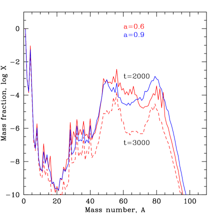
Figure 11.— Volume integrated abundance distribution of elements synthesized in the accretion disk in 2D simulation with The black hole spin in the simulation was $a=0.9$ (blue line), and $a=0.6$ (red lines). The distributions of density, temperature, and electron fraction in the flow were taken at two time snapshots: $t=2000M$ and $t=3000M$, as marked with solid and dashed lines, respectively.

The second setup corresponds to a bright GRB scenario, when the power available from the Blandford-Znajek process is 100 times higher, than in the first case, and also the power from the neutrino annihillation is almost 3 times higher. In this engine, similarly to the previous one, there will be produced isotopes of Iron and Vanadium, as well as Selenium, Manganese, Strontium, and Krypton. The latter are about 10 times more abundant, than in the case of a faint GRB engine, and they can be produced efficiently in the engine for a longer time.

The isotopes synthetized in the GRB central engine accreting torus and its outflows during the prompt emission phase, should be detectable via the X-ray emission that originates from their radioactive decay. These isotopes, such as ${}^{45}Ti$, ${}^{57}Co$, ${}^{58}Cu$, ${}^{62}Zn$, ${}^{65}Ga$, ${}^{60}Zn$, ${}^{49}Cr$, ${}^{65}Co$, ${}^{61}Co$, ${}^{61}Cu$, and ${}^{44}Ti$, might give the signal in the 12-80 keV energy band, which could in principle be observed by current instruments with a good energetic resolution, such as e.g., NuSTAR.

5. Summary and discussion

We calculated the structure and short-term evolution of a gamma ray burst central engine in the form of a magnetized torus accreting onto a black hole. Our computations were performed in a fixed background metric around a spinning black hole, and the physical conditions in the plasma driven by the hyper-Eddington accretion rate were taken into account by the adopted microphysics. We describe the flow properties using the numerical equation of state of dense and hot matter, where the free nucleons and electron-positron pairs are relativistic and partially degenerate. We estimate the resulting neutrino luminosity, which cools the flow via the nuclear reactions in which neutrinos of the three flavors are produced. We conclude that the total integrated luminosity is larger than the power possibly extracted from the rotating black hole via the Blandford-Znajek process. Taking into account the uncertainty of the efficiency of the neutrino anihillation in the bi-polar jets (Zalamea & Beloborodov, 2011), we still find that the power supply to the jets by neutrinos is plausible and energetically competitive to the magnetic extraction of the black hole rotation energy.

The discussion of interplay between the Blandford-Znajek mechanism versus neutrino power supply to the GRB jets has been proposed in a number of works based on the so-called NDAF disk, e.g., Liu et al. (2015). These conclusions are however far from robust, regarding the very simplified treatment of accretion flows in these models, which is described by a classical 1-dimensional steady state accretion flow with $\alpha$ viscosity, and pseudo-Newtonian gravity. Our computations realistically treat the nuclear equation of state, together with other relevant physical ingredients, like the general relativity and magnetic fields. The latter is still lacking in some of the otherwise advanced, three-dimensional dynamical simulations of neutrino-cooled accretion flows in the short GRB engines (Dessart et al. , 2009; Perego et al. , 2014). The essentially inviscid nature of such models might lead to their somewhat underestimated results for the accretion speed, dissipation and cooling rates.

On the other hand, the relativistic models which are based on the ideal gas EOS (e.g., Rezzolla et al. (2011) use the adiabatic EOS with index of 2), can predict overestimated profiles of the disk scaleheight. Also, as noted by Kiuchi et al. (2015), who use the gamma index of 1.8 in their accretion flow computations, the value of this index will affect the amount of matter ejected in the torus wind. By accounting for the proper microphysics, instead of the simplistic EOS, we can get therefore most reliable description of the conditions in neutrino driven winds. The exact determination of the accretion disk thickness is crucial with respect to the possible gravitational or thermal instabilities (Perna et al. , 2006; Janiuk et al. , 2007), which can lead to the episodic accretion events and hence observable flares. As it was shown by Begelman & Pringle (2007), the strong magnetic fields can be important for the stabilisation of the accretion flow against self-gravity. The ordered magnetic field configuration, which is mostly toroidal in the accretion torus with but predominantly poloidal and jet-like along the BH spin axis, is produced in simulation of Rezzolla et al. (2011) at time about 6 ms after the black hole formation. In our simulations the poloidal field lines appear after about 15 ms for the black hole of a 3 $M_{\odot}$, so the results are consistent within an order of magnitude. The difference in the timescale may be connected to some extent with the interplay between magnetic field dynamics and gas properties, but also affected by the 2-dimensional setup which is used in our model. We plan to expand the current computations into 3-dimensions in the future work, and then test quantitatively the resulting models against the observables of GRBs, such as their time variability, duration, and energetics. The ultimate impact of such simulations can also lead to the constraints on the magnetic fields strengths and configuration in the cosmic environment related to GRB progenitors.

Finally, based on the computed structure of the flow, its density, temperature, and electron fraction, we are able to estimate the integrated abundances of heavy elements which are synthetized in the flow via the subsequent nuclear reaction chain. These elements, if decaying radioactively at some distance from the central engine, will then contribute to the heating of the circum-burst medium, and afterglow emission.

As shown by Sekiguchi et al. (2015), the dynamical ejecta including neutrino transport may develop the shock waves, and related heating is responsible for enhanced reaction rates. The electron fraction is then increased, and their nuclear reaction networks are able to produce the r-process elements up to A=195. This was however not encountered in the Newtonian simulations, which produce elements up to A=130 (Goriely et al. , 2011). Neutron star mergers are therefore expected to produce significant quantities of neutron-rich radioactive species, whose decay should result in a faint transient emission. The latter is called a ‘kilonova’, and should appear in the days following the burst. The term refers to the luminosity peak in the near infrared band, rather than UV or Optical (Li & Paczynski , 1998), and the emission produced in the regions of the opacities much higher than in the case of of supernovae. An observational support for such event has been reported e.g. by Tanvir et al. (2013) for a short duration GRB 130603B. Recently, re-examination of the observed long burst emission in GRB 060614 has shown that it is consistent with the ’kilonova’ scenario, rather than an undelying supernova (Yang et al. , 2015).

The gamma ray bursts can play a unique role in the metal enrichment of the Universe, as they are the brightest sources at all redshifts, and, for long GRBs, they occur in the star forming regions. Because the nucleosynthesis yields from the explosions of stars in different populations could differ by orders of magnitude, the metal abundance patterns, imprinted in the interstellar medium, should depend on the initial mass function (Heger & Woosley , 2010). The abundance patterns measured with distant GRBs can be used to determine the typical masses of the early stars (Pop III), and disentangle them from the younger Pop II SNe. Such studies are planned e.g. with the newly developing instruments, e.g., on-board the Athena X-ray satellite, which is aiming to probe the GRB afterglow spectra, in combination with the studies of the quasars on the line of sight (Jonker et al. , 2013). The GRBs can be observed up to the highest redshifts (e.g., z=9.4, for GRB 090429, Cucchiara et al. (2011)) and hence the old stellar populations can be traced in their X-ray afterglow spectra, e.g., with absorption lines of Fe, Mg, Si, S, Ar, from the ionized gas in the GRB environment. Nevertheless, these data can be contaminated by the effects of the intergalatic medium and hence the observed absorption column is a combined effect of the warm-hot intergalactic medium, Lyman alpha clouds, as well as the circumburst medium intrinsic to the host galaxy (Starling et al. , 2013).

From the point of view of stellar evolution models, Heger & Woosley (2010) computed the nucleosynthesis yields of elements produced in the massive metal-free stars, but they ignored both the neutrino-powered winds and the gamma-ray bursts accretion disks. The latter, as studied by Surman et al. (2006), have large overproduction factors in their outflows for the nuclei like ${}^{44}Ti$, ${}^{45}Sc$, and ${}^{64}Zn$. Also, the light p-nuclei, such as ${}^{92}Mo$, and ${}^{94}Mo$, are produced in the rapidly accreting disks, as found by Fujimoto et al. (2003)). The neutrino-driven winds, on the other hand, were modeled recently by Perego et al. (2014) in the context of binary neutron star mergers. They found that the wind can successfully contribute to the weak r-process in the range of atomic masses from 70 to 110.

Obviously, the long GRBs are only a fraction of the massive star explosions and luminous supernovae (Guetta & Della Valle , 2007; Hjorth & Bloom , 2012), and their impact for the majority of elements may not be crucial. However, verifying the signatures of these elements which are produced mainly in the GRB engines, may in the future occur to be a prospective tool to study the chemical evolution in the Universe due to the collapsing massive stars, via the available GRB afterglow X-ray spectra. Also, some of the bursts may be connected with peculiar type of events, such as the burst GRB 111209A/SN 2011kl (Kann et al. , 2016). In such case, the conditions in GRB central engine, determined during the explosion, can also lead to peculiar distributions of electron fraction, and affect the synthesis process for neutron-rich isotopes.

Table 2Summary of the models with a massive black hole, $M_{\rm BH}=62M_{\odot}$, as estimated for the first LIGO-detected black hole. The mass of the torus is given in $M_{\odot}$, accretion rate in $M_{\odot}$s^-1, the time is in seconds, and luminosity in erg s^-1.

Model	$a$	$R_{\rm max}$	$t_{\rm e}$	$M_{\rm t}(t_{0})$	$M_{\rm t}(t_{\rm e})$	$<\dot{M}>$	$\dot{M}(t_{\rm e})$	$L^{\rm tot}_{\nu}(t_{\rm e})$	$L_{\rm BZ}(t_{\rm e})$
lbhAc	0.6	9.1	0.91	16.8	14.36	5.01	4.06	$4.80\times 10^{53}$	0
lbhBc	0.7	8.4	0.91	13.0	11.17	4.64	1.99	$6.18\times 10^{53}$	0
lbhCc	0.8	7.5	0.92	10.6	9.02	4.07	3.59	$6.60\times 10^{53}$	$1.93\times 10^{51}$
lbhDc	0.9	7.0	0.91	10.4	8.89	3.98	2.55	$9.72\times 10^{53}$	$3.30\times 10^{51}$
lbhEc	0.98	6.6	0.91	16.4	15.23	2.93	1.85	$5.64\times 10^{54}$	$3.31\times 10^{52}$

The synthesized heavy elements can also be the source of a faint emission of a kind of an ’orphan’ afterglow, if the main GRB jet is directed off-axis, or it is intrinsically very weak in its gamma ray fluence. Still, the detection of such an afterglow emission will be a hint of the existence of a black hole in the engine site. Measurements of nucleosynthesis signatures may therefore help constrain the model parameters for such engine, namely the black hole spin and its mass.

The recent detections of the gravitational wave signal (Abbott et al. , 2016) confirmed independently the existence of black holes in the Universe. The analysis of the gravitational wave signal allows to constrain the black hole mass and spin (with some uncertainty). In the case of the source GW150914, it was found that the signal is related to the merger of a binary black hole. So far, the electromagnetic counterpart for this first event was tentatively reported only by Fermi satellite, who gave a limit for detection of a weak gamma ray signal (Connaughton et al. , 2016). No infrared emission was reported, and also the signal was not confirmed by other gamma-ray missions for the case of this burst (Greiner , 2016).

Nevertheless, the detection of the electromagnetic counterpart of a gravitational wave source in the future events is appealing. The related estimates for the heavy elements synthesized in the ejecta could help constrain the parameters for the GRB engine, if the latter happens to coincide with the gravitational wave source. In particular, if the binary black holes merge within a remnant circumbinary disk, which is a leftover after the past supernova explosion (Perna et al. , 2016), then the nucleosynthesis of elements within the disk engine and ejected winds can also be responsible for an infrared counterpart. Direct measurements of the escaping gamma-rays, which will be produced at larger distance in the r-process nucleosynthesis, are probably difficult with current X-ray and gamma-ray missions (Hotokezaka et al. , 2016).

The black hole, which was the product of the merger of two black holes of about 29 and 36 Solar mass black holes, was also a moderately spinning one. The constraints for its dimensionless spin parameter obtained from the amplitude and phase evolution of the observed gravitational waveform gave a value of $0.67^{+0.05}_{-0.07}$, while the final black hole mass was equal to $62^{+4}_{-4}\ M_{\odot}$. As can be shown, such a binary black hole merger, if accompanied by the matter accretion onto a rotating black hole, which happens either before, or after the merger, can lead to an unusual gamma ray burst (Janiuk et al. , 2013b, 2017). In the case of the relatively small rate of the black hole rotation, such as in GW150914, the accretion will result in a very small electromagnetic flux dragged through the black hole horizon and hence a negligibly small power of the Blandford-Znajek process.

We computed an additional set of the gamma ray burst engine models, with parameters taken to be representative for the above scenario (see Table 2).

Figure 12.— Heavy elements synthesized in the torus and its wind, for the model lbhBc and lbhDc in the Table 2. The black hole mass is $M_{\rm BH}=62M_{\odot}$, and its spin is a=0.9 (blue), or a=0.7 (red). The torus mass is about 15 $M_{\odot}$ and results were taken at time $t=2000M$ in the dynamical simulation.

We have also computed the mass fraction distribution of heavy elements produced in this putative engine (Figure 12). We found, that contrary to the presented in the previous Section ’fiducial’ models, with a standard (small) black hole mass and accretion torus, here the nuclear conditions preferably lead to production of mainly Iron peak elements. In the model lbhD (see Table 2), the mass fraction of Iron 56 reached almost 1.0, while the isotopes from the group of Selenium and Manganese were $10^{3}$ times less abundant. This result suggests a possible additional test for the conditions present in the GRB engine, e.g., if the event happened to be coincident with a merger of the two $\sim 30M_{\odot}$ black holes with masses of about $\sim 30M_{\odot}$ each. It is also worth to notice that the supernova explosion which might have left a 30 Solar mass black hole, should have originated from at least 80 Solar mass star on zero-age main sequence, in a low-metallicity environment (Spera et al. , 2015). Even if a significant amount of the star’s mass was ejected during the evolution and explosion, some remnant disk is plausible, but detailed modeling of its structure should be also confronted with the supernova theory.

More generally, the gravitational waves discovery, GW150914, may reveal the new population of weak gamma ray bursts originating from the low Lorentz factor jets. In this case, the prompt electromagnetic emission may be difficult to discover, but the observation of a radioactive decay of elements produced in the engine of the GRB may be confronted with the engine simulation predictions. The black hole parameters, namely its spin and mass, determine the shape of the gravitational wave signal and hence can be independently constrained. As shown in Figure 12, the results for nucleosynthesis yields somewhat depend on the black hole spin value. The abundance of isotopes produced in the accreting torus around a faster spinning black hole, is about 10 times higher at about $A=80$ (Selenium group) than for a slowly spinning black hole. Thus, the predictive power of our models is worth exploring in the future work, if only the accreting black hole parameters are determined and the nucleosynthesis yields constrained with some future observations, i.e. X-ray probes.

References

- Abbott et al. (2016) Abbott, et al., 2016, Phys. Rev. Lett., 116.061102
- Abramowicz et al. (1978) Abramowicz M.A., Jaroszynski M., Sikora M., 1978, A&A, 63, 221
- Barkov & Baushev (2011) Barkov, M.V., Baushev, A.N., 2011, New Astr., 16, 46
- Barkov & Komissarov (2010) Barkov, M.V., Komissarov, S.S., 2010 MNRAS, 401, 1644
- Begelman & Pringle (2007) Begelman M., Pringle J., 2007, MNRAS, 375, 1070
- Blandford & Znajek (1977) Blandford, R.D., Znajek, R.L., 1977, MNRAS, 179, 433
- Bromberg & Tchekhovskoy (2016) Bromberg, O., Tchekhovskoy, A., 2016, MNRAS, 456, 1739
- Cao et al. (2014) Cao X.-W., Liang E.-W., Yuan Y.-F., 2014, ApJ, 789, 129
- Chen & Beloborodov (2007) Chen W.-X. & Beloborodov A., 2007, ApJ, 657, 383
- Connaughton et al. (2016) Connaughton V., et al., 2016, arXiv:1602.03920
- Cucchiara et al. (2011) Cucchiara A., Levan A.J., Fox D.B., et al., 2011, ApJ, 736, 7
- Dessart et al. (2009) Dessart L., Ott C. D., Burrows A.; Rosswog S., Livne E., 2009, ApJ, 690, 1681
- Di Matteo et al. (2002) Di Matteo T., Perna R., Narayan R., 2002, ApJ, 579, 706
- Fishbone & Moncrief (1976) Fishbone L.G., Moncrief V., 1976, ApJ, 207, 962
- Fujimoto et al. (2003) Fujimoto, S., Hashimoto, M., Koike, O., Arai K., Matsuba R., 2003, ApJ, 585, 418
- Fujimoto et al. (2004) Fujimoto, S., Hashimoto, M., Arai, K., Matsuba, R., 2004, ApJ, 614, 847
- Gammie et al. (2003) Gammie C.F., McKinney J.C. & Toth G., 2003, ApJ, 589, 444
- Goriely et al. (2011) Goriely, S., Bauswein, A., Janka, H.-Th., 2011, ApJ, 738, L32
- Greiner (2016) Greiner, J., Burgess J. M., Savchenko V., Yu H.-F., 2016, ApJ, 827, L38
- Guetta & Della Valle (2007) Guetta D., Della Valle M., 2007, ApJ, 657, L73
- Heger & Woosley (2010) Heger A., Woosley S.E., 2010, ApJ, 724, 341
- Hix & Meyer (2006) Hix W.R., Meyer B.S., 2006, Nucl Phys., 777, 188
- Hjorth & Bloom (2012) Hjorth J., Bloom J.S., 2012, Chapter 9 in ”Gamma-Ray Bursts”, Cambridge Astrophysics Series 51, eds. C. Kouveliotou, R. A. M. J. Wijers and S. Woosley, Cambridge University Press (Cambridge), p. 169-190
- Hotokezaka et al. (2016) Hotokezaka, K.; Wanajo, S.; Tanaka, M.; Bamba, A.; Terada, Y.; Piran, T., 2016, MNRAS, 459, 35
- Ibanez et al. (2015) Ibanez, J.-M., Cordero-Carrión I., Aloy M.-A., Marti J.-M., Miralles J.-A., 2015, Class Q. Grav, 32, 095007
- Janiuk et al. (2004) Janiuk, A.; Perna, R., Di Matteo, T.; Czerny, B., 2004, MNRAS, 355, 950
- Janiuk et al. (2007) Janiuk A., Yuan Y.-F., Perna R., Di Matteo T., 2007, ApJ, 664, 1011
- Janiuk & Yuan (2010) Janiuk A., Yuan Y.-F., 2010, A&A, 509, 55
- Janiuk et al. (2013) Janiuk A., Mioduszewski P., Moscibrodzka M., 2013, ApJ, 776, 105
- Janiuk et al. (2013b) Janiuk A., Charzynski S., Bejger M.., 2013, A&A, 560, 25
- Janiuk (2014) Janiuk A., 2014, A&A, 568, 105
- Janiuk et al. (2017) Janiuk A., Bejger M., Charzynski S., Sukova P., 2017, New Astr., 51, 7
- Jonker et al. (2013) Jonker P., O’Brien P., Amati L., et al., Supporting paper for the science theme ”The Hot and Energetic Universe” to be implemented by the Athena+ X-ray observatory (http://www.the-athena-x-ray-observatory.eu), (arXiv:1306.2336)
- Kann et al. (2016) Kann D.A., et al., 2016, submitted arXiv:1606.06791
- Kluzniak & Lee (1998) Kluzniak W., Lee W.H., 1998, ApJ, 494, 53
- Kohri & Mineshige (2002) Kohri, K., Mineshige, S., 2002, ApJ, 577, 311
- Kohri et al. (2005) Kohri, K.; Narayan, R.; Piran, T., 2005 ApJ, 629, 341
- Kumar & Zhang (2015) Kumar P., Zhang B., 2015, Phys. Reports, 561, 1.
- Kiuchi et al. (2015) Kiuchi, K., Sekiguchi, Y., Kyutoku, K., Shibata, M., Taniguchi, K., Wada, T., 2015, Phys. Rev. D, 92, 064034
- Li & Paczynski (1998) Li, L.-X., Paczynski, B., 1998, ApJ, 507, L59
- Lopez-Camara et al. (2009) Lopez-Camara D., Lee W.H., Ramirez-Ruiz E., 2009, ApJ, 692, 804
- Lee & Ramirez-Ruiz (2007) Lee W.H., Ramirez-Ruiz E., 2007, New Journal of Physics, 9, 17
- Lee et al. (2009) Lee W.H., Ramirez-Ruiz E., Lopez-Camara D., 2009, ApJ, 699, L93
- Lei et al. (2009) Lei W. H., Wang D. X., Zhang L., Gan Z.M., Zou Y. C., Xie Y., 2009, ApJ, 700, 1970
- Liu et al. (2015) Liu T., Lin Y.-Q., Hou S., Gu W.-M., 2015, ApJ, 806, L58
- Martin et al. (2015) Martin, D.; Perego, A.; Arcones, A.; Thielemann, F.-K.; Korobkin, O.; Rosswog, S., 2015, ApJ, 813, 2
- McKinney & Gammie (2004) McKinney J.C., Gammie C.F., 2004, ApJ, 611, 977
- McKinney (2006) McKinney J.C., 2006, MNRAS, 368, 1561
- McKinney & Blandford (2009) McKinney J.C., Blandford R., 2009, MNRAS, 394, L126
- McKinney, Tchekhovskoy & Blandford (2012) McKinney J.C., Tchekhovskoy A., Blandford R. D., 2012, MNRAS, 423, 3083
- Meyer (1994) Meyer, B. S., 1994, ARA&A, 32, 153
- Moscibrodzka & Falcke (2013) Moscibrodzka M., Falcke H., 2013, A&A, 559, L3
- Nagataki (2009) Nagataki S., 2009, ApJ, 704, 937
- Narayan et al. (2000) Narayan R., Piran T., Kumar P., 2000, ApJ, 557, 949
- Noble et al. (2006) Noble S.C., Gammie C.F., McKinney J.C., & Del Zanna L., 2006, ApJ, 641, 626
- Paczynski (1998) Paczynski B., 1998, ApJL, 494, 45
- Paschalidis et al. (2011) Paschalidis V., Etienne Z., Liu Y.T., Shapiro S.L., 2011, Phys. Rev. D, 83, 064002
- Perego et al. (2014) Perego A., Rosswog S., Cabezon R.M., et al., 2014, MNRAS, 443, 3134
- Perna et al. (2006) Perna R., Armitage P., Zhang B., 2006, ApJ, 636, 29
- Perna et al. (2016) Perna R., Lazzati D., Giacomazzo B., 2016, ApJ, 821, L18
- Piran (2004) Piran T., 2004, Reviews of Modern Physics, 76, 1143
- Popham et al. (1999) Popham, R.; Woosley S.E.; Fryer, C., 1999, ApJ, 518, 356
- Reynoso et al. (2006) Reynoso, M. M.; Romero, G. E.; Sampayo, O. A., 2006, A& A, 454, 11
- Reddy et al. (1998) Reddy S., Prakash M., Lattimer J.M., 1998, Phys. Rev. D, 58, 013009
- Rezzolla et al. (2011) Rezzolla L., Giacomazzo B., Baiotti L., et al., 2011, ApJ, 732, 6
- Schwab et al. (2012) Schwab J., Shen, K.J., Quataert E., Dan M., Rosswog S., 2012, MNRAS, 427, 190
- Sekiguchi et al. (2015) Sekiguchi, Y., Kiuchi, K., Kyutoku, K., Shibata, M., 2015, Phys. Rev D, 91, 064059
- Seitenzahl et al. (2008) Seitenzahl, I. R., Timmes, F. X., Marin-Laflèche, A., et al. 2008, ApJL, 685, 129
- Shibata et al. (2007) Shibata M., Sekiguchi Y., Takahashi R., 2007, Progress of Theoretical Physics, 118, 2
- Shibata et al. (2011) Shibata M., Taniguchi K., 2011, ApJL, 734, L36
- Shibata & Taniguchi (2011) Shibata M., Suwa Y., Kiuchi K., Ioka K., 2011, Living Rev. in Relativity, 14, 6
- Spera et al. (2015) Spera M., Mapelli M., & Bressan A., 2015, MNRAS, 451, 4086
- Starling et al. (2013) Starling R.L.C., Willingale R., Tanvir N.R., et al., 2013, MNRAS, 431, 3159
- Surman et al. (2006) Surman R., McLaughlin G.C., Hix W.R., 2006, ApJ, 643, 1057
- Surman et al. (2014) Surman R., Caballero O.L., McLaughlin G.C., Just O., Janka H.-Th., 2014, J. Phys. G, 41, 044006
- Tanvir et al. (2013) Tanvir, N.R., Levan, A. J., Fruchter, A. S., Hjorth, J., Hounsell, R. A., Wiersema, K., Tunnicliffe, R. L. 2013, Nature, 500, 547
- Tchekhovskoy et al. (2008) Tchekhovskoy, A., McKinney, J.C., Narayan, R., 2008, MNRAS, 388, 551
- Tchekhovskoy & Bromberg (2016) Tchekhovskoy, A., Bromberg O., 2016, MNRAS, 461, L46
- Wallerstein et al. (1999) Wallerstein, G. et al., 1997, Rev. Mod. Phys., 69, 995
- Woosley (1993) Woosley S.E., 1993, ApJ, 405, 273
- Yang et al. (2015) Yang B., Jin Z.P., Li X., et al., Nature Comm., 6, 7323
- Yuan (2005) Yuan Y.-F., 2005, Phys. Rev. D, 72, 013007
- Zalamea & Beloborodov (2011) Zalamea I., Beloborodov A.M., MNRAS, 410, 2302