From 6D SCFTs to Dynamic GLSMs

Abstract

Compactifications of 6D superconformal field theories (SCFTs) on four-manifolds generate a large class of novel 2d quantum field theories. We consider in detail the case of the rank one simple non-Higgsable cluster 6D SCFTs. On the tensor branch of these theories, the gauge group is simple and there are no matter fields. For compactifications on suitably chosen Kähler surfaces, we present evidence that this provides a method to realize 2d SCFTs with $\mathcal{N}=(0,2)$ supersymmetry. In particular, we find that reduction on the tensor branch of the 6D SCFT yields a description of the same 2d fixed point that is described in the UV by a gauged linear sigma model (GLSM) in which the parameters are promoted to dynamical fields, that is, a “dynamic GLSM” (DGLSM). Consistency of the model requires the DGLSM to be coupled to additional non-Lagrangian sectors obtained from reduction of the anti-chiral two-form of the 6D theory. These extra sectors include both chiral and anti-chiral currents, as well as spacetime filling non-critical strings of the 6D theory. For each candidate 2d SCFT, we also extract the left- and right-moving central charges in terms of data of the 6D SCFT and the compactification manifold.

1 Introduction

One of the notable predictions of string theory is the existence of 6D superconformal field theories (SCFTs) [1, 2, 3]. Though a microscopic formulation of these theories remains elusive, it is especially remarkable that upon compactification to lower dimensions, simple geometric operations of the compactification space lead to highly non-trivial dualities. This includes the well-known case of compactification of the $(2,0)$ SCFTs on a $T^{2}$, and the corresponding S-duality of $\mathcal{N}=4$ Super Yang-Mills theory [4, 5]. Compactifying on Riemann surfaces with punctures leads to $\mathcal{N}=2$ dualities [6, 7, 8]. Similar considerations hold for compactification to three, two and one dimension (for a partial list of examples, see [9, 10, 11, 12, 13]).

It is natural to ask whether similar structures persist for compactifications of 6D SCFTs with minimal, i.e., $(1,0)$ supersymmetry. Recent work on 6D SCFTs with a tensor branch [14, 15, 16, 17, 18, 19, 20] has produced a classification of nearly all such theories. See also [24, 25] for a classification of theories with a holographic dual.

Compactifications of these $(1,0)$ SCFTs to lower dimensions have the potential to provide access to strong coupling dynamics in the resulting lower-dimensional theories. One complication is that due to the reduced amount of supersymmetry, any such theory will be subject to more quantum corrections than their $(2,0)$ counterparts. Nevertheless, it is still possible to extract some data for the 4d theories obtained from compactification, as in references [26, 27, 28, 29, 30, 31, 32, 33, 34, 35, 36].

In this work we begin the study of the resulting 2d effective theories obtained by compactification of $(1,0)$ SCFTs on a four-manifold. We find that the resulting 2d theories are often 2d SCFTs, and moreover, are characterized by an appropriate UV gauged linear sigma model (GLSM) in which some of the parameters of the model are promoted to dynamical chiral and anti-chiral bosons. These gauge theories are often coupled to additional chiral / anti-chiral currents as well as spacetime filling strings of the 6D theory (see figure 1 for a depiction). We also use this geometric characterization to produce parametric families of 2d SCFTs.

Now, although these $(1,0)$ theories have reduced supersymmetry when compared with their $(2,0)$ counterparts, this is compensated by the fact that the theory on the tensor branch typically has more structure. One of the central points of this work will be to exploit this description on the tensor branch to achieve a better understanding of the microscopic ingredients of the resulting 2d effective field theories. Figure 2 shows the different RG flow trajectories: we can either directly compactify our 6D SCFT on a four-manifold, reaching a 2d effective theory, or we can first flow on the tensor branch and then compactify the theory on this branch, yielding an a priori different 2d effective theory. In spite of their differences in six dimensions, we will present evidence that the two a priori different 2d theories obtained from compactification are in fact one and the same.

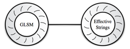
Figure 1: Compactification of the tensor branch deformation of a 6D SCFT on a four-manifold yields a DGLSM, i.e. a gauged linear sigma model in which the couplings are dynamical. These theories are also coupled to chiral / anti-chiral currents and spacetime filling strings.

Indeed, for $(1,0)$ theories, the tensor branch is governed by a weakly coupled 6D gauge theory coupled to tensor multiplets and possibly exotic matter fields. The scalar of the tensor multiplet promotes the gauge coupling to a dynamical field, and the 6D anti-chiral two-form potential is crucial for 6D anomaly cancellation via the Green-Schwarz mechanism [37, 38, 39, 40].

Upon compactification on a four-manifold, the 6D vector multiplet and matter fields reduce to fields present in a 2d non-abelian GLSM. More striking, however, is that the gauge coupling of the GLSM will be dynamical, and the anti-chiral two-forms will reduce to 2d chiral and anti-chiral bosons which couple to the fields of the GLSM. Additionally, the presence of spacetime filling effective strings (as dictated by the tadpole for the anti-chiral two-form) provides additional chiral sectors which couple to the GLSM.

What then is the relation of this 2d theory to the one obtained by directly compactifying the 6D SCFT on a four-manifold? We propose the following answer. There is one theory with dynamical couplings that depends on fields of an underlying non-linear sigma model with non-compact target space. The target space is non-compact due to unsuppressed contributions of large values of the tensor scalar field, and precisely in this regime we have a description in terms of a weakly coupled theory fibered over the non-linear sigma model target space. Of course no such weakly coupled description can be given at the origin of the tensor branch, and experience with similar strongly coupled systems might at first suggest these two theories are at infinite distance from one another. On the contrary, we will present evidence that the origin is at finite distance in the target space metric.

The primary evidence we provide comes from compactifying on a Kähler surface, where we expect to get a 2d SCFT with $(0,2)$ supersymmetry. In this case, we can calculate the anomaly polynomial for the 2d theory by dimensional reduction of the 6D answer. We compare this with the anomaly polynomial obtained from reduction of the 6D theory on the tensor branch, and we obtain a perfect match.

The fact that this picture hangs together in a consistent fashion also helps to address questions of interest in a purely 2d context. For example, although $(0,2)$ GLSMs are widely studied, the case where the parameters of the model are promoted to dynamical fields (let alone chiral fields) is not well understood, even though, as we discuss below, it is actually the generic case! While there are many such theories one might write down, a priori it is entirely unclear which of them will yield sensible results. The top–down approach provides us with candidates with which we can begin to explore this wider world of 2d dynamics, and even in these relatively simple theories, we find a rich structure including the following features:

1. Gauge degrees of freedom with dynamical couplings.

2. A non-compact target space and therefore no normalizable vacuum state.

3. A rich current algebra, part of which is gauged, that originates from reduction of the 6D anti-chiral two-form.

4. Marginal couplings that originate from the geometry of the compactification manifold.

Figure 2: Depiction of the different theories starting from compactification of a 6D theory. We can either begin with a 6D SCFT and compactify directly to two dimensions, obtaining a strongly coupled candidate 2d SCFT indicated by $\ast$. Alternatively, we can instead consider compactification of the 6D theory far out on its tensor branch, arriving at a weakly coupled dynamic GLSM (the coupling is indicated by the radius of the circle) fibered over the tensor non-linear sigma model. The match in anomalies for the two 2d theories so obtained suggests that $\ast$ is at finite distance in the appropriate sigma model metric.

To provide more details of this picture, our focus in this work will be on compactification of a class of 6D SCFTs we refer to as “simple non-Higgsable clusters.” The non-Higgsable clusters (NHCs) of reference [41] are the building blocks used in the construction of all 6D SCFTs via F-theory [14, 19]. In F-theory terms, these theories are characterized by a collection of $\mathbb{P}^{1}$’s in the base such that the generic elliptic fibration over these curves is singular. Non-Higgsable clusters consist of up to three $\mathbb{P}^{1}$’s, with the specific configuration of gauge groups and matter fully dictated by the self-intersection of the curve. In particular, the simple NHCs (SNHCs) consist of a single $\mathbb{P}^{1}$ of self-intersection $-n$ with $n\in\{3,4,6,8,12\}$. For these choices, the gauge group is simple and there are no matter fields. An additional feature of these cases is that the F-theory model can be written (for appropriate moduli) as an orbifold $\mathbb{C}^{2}\times T^{2}/\mathbb{Z}_{n}$.

Reduction of the 6D Green-Schwarz terms leads to an intricate anomaly cancellation mechanism in two dimensions for these theories. In addition to the chiral and anti-chiral bosons obtained from reduction of the 6D anti-chiral two form, we also find spacetime filling strings. These theories are in turn defined by the dimensional reduction of a strongly coupled $\mathcal{N}=2$ superconformal field theory on $\mathbb{R}^{1,1}\times\mathbb{P}^{1}$. The number of such spacetime filling strings is dictated by the precise coefficients appearing in the 6D Green-Schwarz terms. For recent work on the structure of these spacetime filling strings, see references [42, 43, 44, 45].

To perform precision checks on our proposal, we also specialize to the case of a Kähler surface so that the resulting 2d effective theory enjoys $(0,2)$ supersymmetry. In this case, a putative superconformal field theory will have a $U(1)$ R-symmetry. Assuming the absence of emergent abelian symmetries in the infrared, this R-symmetry descends from symmetries already present in the 6D description. For the simple NHCs there are in fact no continuous flavor symmetries – abelian or non-abelian – in six dimensions. This in particular makes an analysis of the infrared R-symmetry particularly tractable. Matching all of the data of the anomalies including the infrared R-symmetry, we obtain a non-trivial match between the two a priori different 2d theories.

The fact that the anomalies of the two theories match is a strong indication that we are simply describing the same branch of a single SCFT. While it is indeed quite plausible that compactifying a 6D SCFT will produce a 2d SCFT, it is quite non-trivial that the massive tensor branch flows back to the same fixed point upon further compactification. We take this to mean that the distinction between these two theories is erased once we integrate out the massive Kaluza-Klein states.

Indeed, from the perspective of the F-theory realization of these models, in both phases we have a seven-brane wrapped over a Kähler threefold $M_{4}\times\mathbb{P}^{1}$. To reach the compactification of the 6D SCFT, we first collapse the $\mathbb{P}^{1}$ factor to zero size. To instead reach the DGLSM description, we first collapse $M_{4}$ to zero size. This also motivates a physical picture in which the complexified geometric moduli of $M_{4}$ parameterize a family of 2d SCFTs.

The rest of this paper is organized as follows. First, in section 2, we introduce the class of 6D SCFTs we shall study, i.e. the simple NHCs. We also study the twist of the 6D SCFT, and the reduction of the anomaly polynomial to two dimensions. One of our goals will be to reproduce this answer directly from the 2d theory obtained from reduction on the tensor branch. Next, in section 3 we discuss some general aspects of DGLSMs, and in particular how the 6D perspective helps in understanding various aspects of the quantum dynamics. In section 4 we turn to the explicit F-theory realization of DGLSMs. Section 5 shows that all gauge anomalies for the DGLSMs vanish, and moreover, calculates the anomaly polynomial for the resulting theories wrapped on a Kähler surface. We present our conclusions and directions for future investigation in section 6. Some additional details on the reduction of free 6D supermultiplets to two dimensions are given in Appendix A. Additional details on the spacetime filling strings of the simple NHCs are provided in Appendix B.

2 6D SCFTs on a Four-Manifold

In this section we review some of the salient points of 6D SCFTs, and their compactification on a four-manifold. The primary evidence for the existence of higher-dimensional conformal fixed points comes from string theory, so we shall mainly adhere to stringy conventions in our construction and study of such models. An important feature of all known 6D SCFTs is that they admit a flow onto a tensor branch where all stringlike excitations have finite tension. This is actually where we realize a string construction, and then by taking an appropriate degeneration limit, we pass to the conformal fixed point.

Our aim will be to study the effective field theory obtained from compactifying a 6D SCFT on a four-manifold. Compactifications of 6D SCFTs with $\mathcal{N}=(2,0)$ supersymmetry have been studied for example in references [12, 46, 47].

Experience from higher-dimensional examples strongly suggests that for suitable compactification manifolds (for example, when the curvature of the internal space is negative), we should expect to realize a 2d superconformal field theory. This is also borne out by the fact that 6D SCFTs with a holographic dual [24, 25] realize, upon compactification on a negatively curved space, an $AdS_{3}$ holographic dual (see e.g. [48, 49, 50, 51, 52]). Even so, due to the non-Lagrangian nature of the UV fixed point, this provides only indirect data about the resulting 2d theory such as various anomalies of global symmetries.

Along these lines, we will also study the tensor branch deformation of the 6D theory. On the tensor branch, the strings of the model couple to anti-chiral two-form potentials with anti-self-dual three-form field strengths. Reduction of this theory to two dimensions thus leads to a 2d supersymmetric gauge theory coupled to additional sectors such as chiral and anti-chiral currents, and spacetime filling strings.

Even though the 6D SCFT and tensor branch are distinct in six dimensions, it is natural to ask how their compactifications are related in two dimensions. Here, the peculiariaties of 2d systems show themselves. Since we expect the tensor branch system to also flow to a 2d SCFT, we will actually get two a priori distinct 2d SCFTs. However, using the 6D perspective, we will also see that the anomalies for these two theories are the same, suggesting that in spite of appearances, we are dealing with a single 2d SCFT. This will lead us to the notion of a “dynamic GLSM,” a construct we discuss further in section 3.

The rest of this section is organized as follows. First, we discuss in general terms how to construct 6D SCFTs via F-theory. We then discuss the partial twist of 6D SCFTs on a four-manifold, and then for the tensor branch deformation of these theories. We then compute the reduction of the 6D anomaly polynomial to two dimensions.

2.1 6D SCFTs from F-theory

To provide concrete examples of 6D SCFTs, we will find it convenient to use the F-theory realization of these models. Recently there has been substantial progress in understanding the general structure of 6D SCFTs via compactifications of F-theory on elliptically fibered Calabi-Yau threefolds.

Recall that in F-theory, we work with a ten-dimensional spacetime, but one in which the axio-dilaton of type IIB string theory can have non-trivial position dependence. For the purposes of engineering 6D superconformal field theories, our primary interest will be spacetimes of the form: $\mathbb{R}^{5,1}\times\mathcal{B}$, where the base $\mathcal{B}$ is a non-compact Kähler surface. To reach a 6D SCFT, we must take some collection of $\mathbb{P}^{1}$’s in $\mathcal{B}$ and simultaneously contract them to zero size at finite distance in moduli space. This in turn requires that the intersection pairing for these $\mathbb{P}^{1}$’s is negative definite [14]. The condition that we have a consistent F-theory background requires that $\mathcal{B}$ is actually the base of a (non-compact) elliptically fibered Calabi-Yau threefold. An important result from [41] is that when the self-intersection $-n$ of the $\mathbb{P}^{1}$ satisfies:

$$3\leq n\leq 12~{},$$ (2.1)

then the elliptic fibration is singular over the curve. The upper bound of $12$ comes about from the condition that we can place the elliptic fiber in standard Kodaira-Tate form. For $n=1,2$ we instead have a generic fiber type which is smooth. Collapsing this $\mathbb{P}^{1}$ generates a 6D SCFT [14, 53].

Each value of $n$ determines a minimal singularity type of the elliptic fiber and thus a 6D effective field theory with a UV cutoff. The effective field theory consists of a single tensor multiplet because there is just one $\mathbb{P}^{1}$. The volume of this $\mathbb{P}^{1}$ is the vev of $t$, the scalar in the corresponding tensor multiplet. Additionally, we have a gauge group, and in some limited cases, matter fields. Let us remark that in addition to the rank one non-Higgsable clusters, there are also NHCs with two and three curves, consisting of related intersection patterns $3,2$ as well as $2,3,2$ and $3,2,2$.

All of the bases which appear in an F-theory model are constructed from “gluing” these NHCs together to form larger structures. In physical terms, this comes from taking the theory on a $-1$ curve, which has $E_{8}$ flavor symmetry, and gauging a product subalgebra. For further details on this gluing procedure in the context of 6D SCFTs, see [14, 19].

We shall primarily focus on this class of theories, and in particular the ones with values $n=3,4,6,8,12$. These are the cases where the seven-brane has a simple gauge group, and there are no matter fields. An additional feature of these cases is that for appropriate moduli, the elliptically fibered Calabi-Yau threefold is simply the orbifold $\mathbb{C}^{2}\times T^{2}/\mathbb{Z}_{n}$ [14, 53]. See table 1 for a list of the simple NHCs.

$n=3$	$n=4$	$n=6$	$n=8$	$n=12$
$SU(3)$	$SO(8)$	$E_{6}$	$E_{7}$	$E_{8}$

Table 1: List of Simple NHCs

2.2 Twisting a 6D SCFT

Suppose then, that we have realized a 6D SCFT via a compactification of F-theory. We now turn to the study of their compactification on a four-manifold $M_{4}$. At first, we consider a general Riemannian four-manifold, though we shall see that to preserve at least $\mathcal{N}=(0,2)$ supersymmetry we will need to specialize to the case of a Kähler surface.

To begin, recall that since we have a field theory, there is a local stress energy tensor. As such, we should expect that with sufficient supersymmetry, it is possible to perform a topological twist of the theory. Recall that a 6D SCFT has an $\mathfrak{su}(2)\simeq\mathfrak{sp}(1)_{R,6D}$ R-symmetry, so in compactifying on a four-manifold, we seek possible ways to retain a covariantly constant spinor on the internal space. The supercharges of the 6D $\mathcal{N}=(1,0)$ theory transform as a symplectic Majorana-Weyl spinor in the representation $(\mathbf{4},\mathbf{2})$ of $\mathfrak{so}(5,1)\times\mathfrak{sp}(1)_{R,6D}$. Making the further decomposition to $\mathfrak{so}(1,1)\times\mathfrak{so}(4)\times\mathfrak{sp}(1)\simeq\mathfrak{so}(1,1)\times\mathfrak{su}(2)_{L}\times\mathfrak{su}(2)_{R}\times\mathfrak{sp}(1)_{R,6D}$, we have the decomposition:

$$\mathfrak{so}(5,1)\times\mathfrak{sp}(1)_{R,6D} \supset\mathfrak{so}(1,1)\times\mathfrak{su}(2)_{L}\times\mathfrak{su}(2)_{R}\times\mathfrak{sp}(1)_{R,6D}$$ (2.2)

$$(\mathbf{4},\mathbf{2}) \rightarrow(+1/2,\mathbf{2},\mathbf{1},\mathbf{2})\oplus(-1/2,\mathbf{1},\mathbf{2},\mathbf{2}).$$ (2.3)

In accord with our 2d $\mathcal{N}=(0,2)$ conventions used in reference [54], we refer to fermions with spin $+1/2$ by a $-$ subscript, i.e. $\lambda_{-}$, and fermions with spin $-1/2$ by a $+$ subscripts, i.e. $\psi_{+}$. To avoid overloading the notation, we shall also sometimes drop these subscripts and respectively write $\widetilde{\lambda}$ and $\psi$, respectively.

To perform a twist, we consider activating a background value for the gauge field associated with the $\mathfrak{sp}(1)$ R-symmetry. Our aim is to activate this field strength in such a way that the combined holonomy for the spin connection and the R-symmetry connection retains a covariantly constant spinor of the uncompactified 2d effective theory. On a general four-manifold, we have available to us the standard “Donaldson twist,” introduced in reference [55]. In terms of representations, we take the diagonal subalgebra of $\mathfrak{su}(2)_{R}\times\mathfrak{sp}(1)_{R,6D}$ which we refer to as $\mathfrak{su}(2)_{\text{diag}}$. The structure group retained is now $\mathfrak{su}(2)_{L}\times\mathfrak{su}(2)_{\text{diag}}$. The 6D supercharge now decomposes as:

$$\mathfrak{so}(5,1)\times\mathfrak{sp}(1)_{R,6D} \supset\mathfrak{so}(1,1)\times\mathfrak{su}(2)_{L}\times\mathfrak{su}(2)_{\text{diag}}$$ (2.4)

$$(\mathbf{4},\mathbf{2}) \rightarrow(+1/2,\mathbf{2},\mathbf{2})\oplus(-1/2,\mathbf{1},\mathbf{3})\oplus(-1/2,\mathbf{1},\mathbf{1}),$$ (2.5)

so that now, our twisted supercharges transform as a vector, and a self-dual two form, and a scalar. We thus conclude that on a general four-manifold, we can twist to retain $\mathcal{N}=(0,1)$ supersymmetry in two dimensions.

To retain $\mathcal{N}=(0,2)$ supersymmetry, we can specialize further to the case where $M_{4}$ is a Kähler surface. Since the structure algebra of the holonomy is now reduced to $\mathfrak{u}(2)=\mathfrak{su}(2)_{L}\times\mathfrak{u}(1)_{R}$, this is tantamount to simply taking a further decomposition of $\mathfrak{su}(2)_{\text{diag}}$ to its Cartan subalgebra:

$$\mathfrak{so}(5,1)\times\mathfrak{sp}(1)_{R,6D} \supset\mathfrak{so}(1,1)\times\mathfrak{su}(2)_{L}\times\mathfrak{u}(1)_{\text{diag}}$$ (2.6)

$$(\mathbf{4},\mathbf{2}) \rightarrow(-1/2,\mathbf{1},\mathbf{0})\oplus(+1/2,\mathbf{2,+1})\oplus(+1/2,\mathbf{2,-1})$$ (2.7)

$$\oplus(-1/2,\mathbf{1},\mathbf{+2})\oplus(-1/2,\mathbf{1},\mathbf{0})\oplus(-1/2,\mathbf{1},\mathbf{-2})$$ (2.8)

so as claimed, we now see two real supercharges which are internally scalars, which are also of the same chirality, i.e. we have $(0,2)$ supersymmetry. We now have a continuous 2d R-symmetry with algebra $\mathfrak{so}(2)_{R,2d}$.

Specializing further, we can also consider the case where $M_{4}$ is Calabi-Yau, (i.e. for compact manifolds we have a K3 surface). In this case, we need not twist the theory at all since the Calabi-Yau space already admits covariantly constant spinors. Indeed, since the structure algebra of the holonomy is now further reduced to $\mathfrak{su}(2)_{L}$, we can effectively perform the same decomposition, but with an additional degeneracy due to the $\mathfrak{sp}(1)$ R-symmetry:

$$\mathfrak{so}(5,1)\times\mathfrak{sp}(1)_{R,6D} \supset\mathfrak{so}(1,1)\times\mathfrak{su}(2)_{L}\times\mathfrak{sp}(1)_{R,6D}$$ (2.9)

$$(\mathbf{4},\mathbf{2}) \rightarrow(+1/2,\mathbf{2},\mathbf{2})\oplus(-1/2,\mathbf{1},\mathbf{2})\oplus(-1/2,\mathbf{1},\mathbf{2}),$$ (2.10)

that is, we have a system with $\mathcal{N}=(0,4)$ supersymmetry and the R-symmetry algebra is now $\mathfrak{so}(4)_{R,2d}$.

For additional details on the explicit decomposition of the various spinor representations, and in particular the relation to 6D $\mathcal{N}=(1,0)$ supermultiplets, we refer the interested reader to Appendix A.

As a brief aside, given the fact that our starting point is a theory with conformal symmetry, one might naturally ask whether there are more general possibilities for retaining a conformal Killing spinor. We leave this interesting possibility for future work, perhaps along the lines of references [56, 57, 58].

2.3 Twisting on the Tensor Branch

For suitable choices of four-manifold, we expect the compactification of the 6D SCFT to realize a 2d SCFT. It is also natural to consider the class of 2d theories obtained by compactifying the tensor branch deformation of this SCFT, which will also lead to a 2d SCFT.

An important aspect of the tensor branch is that it retains the $\mathfrak{sp}(1)_{6D,R}$ R-symmetry of the 6D theory, so that the twisting procedure introduced in the previous section can also be applied in this case as well.

On the tensor branch, we have a 6D effective field theory built from consistently combining tensor multiplets, vector multiplets and hypermultiplets. The field content of these modes is:

Tensor Multiplet $$\text{: }t_{6D}\oplus\psi_{L}\oplus B_{MN}^{(-)}$$ (2.11)

Vector Multiplet $$\text{: }A_{M}\oplus\mu_{R}$$ (2.12)

Hypermultiplet $$\text{: }Q\oplus Q^{c}\oplus\chi_{L},$$ (2.13)

where here, bosons are indicated by latin letters and fermions by greek letters. For the hypermultiplet, the $c$ superscript indicates a complex scalar transforming in the conjugate gauge group representation to $Q$. The subscript $L$ and $R$ refers to whether the fermion has the same (L) or opposite (R) chirality to the 6D supercharge.

In the tensor multiplet, we have $t_{6D}$ a real scalar, $B_{MN}^{(-)}$ an anti-chiral two-form and $\psi_{L}$ a left-handed spinor with the same chirality as our $\mathcal{N}=(1,0)$ supercharge which transforms in the $(\mathbf{4},\mathbf{2})$ of $\mathfrak{so}(5,1)\times\mathfrak{sp}(1)_{6D,R}$. Geometrically, the vacuum expectation value (vev) of $t_{6D}$ is associated with the volume of the $\mathbb{P}^{1}$, and the origin of the tensor branch (where the 6D SCFT resides) comes about from collapsing the $\mathbb{P}^{1}$’s to zero size. The anti-chiral two-form $B_{MN}^{(-)}$ has a three-form field strength which satisfies $H^{(3)}=-\ast_{6}H^{(3)}$.

In a string construction this mode comes about from reduction of the four-form potential of type IIB string theory on this collapsing $\mathbb{P}^{1}$. The relative sign convention is fixed by IIB conventions; there we have a self-dual five-form, so since the $(1,1)$ form $\beta_{\mathbb{P}^{1}}^{(1,1)}$ which is Poincaré dual to the collapsing $\mathbb{P}^{1}$ in the local geometry $\mathcal{O}(-n)\rightarrow\mathbb{P}^{1}$ is anti-self-dual, we can expand:

$$F^{(5)}=H^{(3)}\wedge\beta_{\mathbb{P}^{1}}^{(1,1)},$$ (2.14)

i.e. $F^{(5)}=\ast_{10}F^{(5)}$ descends to our sign convention.

Let us now consider the effects of the twist on the content of the various 6D supermultiplets. We mainly focus on the case of reduction of the tensor multiplet, since this is the most unfamiliar case. We focus on the case of compactification on a general four-manifold, preserving just $\mathcal{N}=(0,1)$ supersymmetry. The remaining cases of $\mathcal{N}=(0,2)$ and $\mathcal{N}=(0,4)$ supersymmetry are obtained from further specialization on the internal index structure of our modes. To this end, we denote by $M$ and $N$ internal vector indices, and $\mu$ a vector index on $\mathbb{R}^{1,1}$. Here, then, is the resulting form content for a tensor multiplet after applying the twist on a general four-manifold:

$$\text{Tensor Multiplet}\text{: }B_{\mu\nu}\oplus(t_{6D}\oplus\psi)\oplus(B_{\mu M}\oplus\widetilde{\psi}_{M})\oplus\left(B_{MN}\oplus\psi_{MN}^{(+)}\right).$$ (2.15)

where in the above, we denote left-handed 2d spinors with decoration by a tilde, and right-handed ones by no tilde. Here, $\psi_{MN}^{(+)}$ transforms as a right-handed fermion and internally as a self-dual two-form on $M_{4}$. In the above, we have grouped the terms according to $\mathcal{N}=(0,1)$ supermultiplets, as indicated by the various parentheses. Note that $B_{\mu\nu}$ does not really pair with a fermion. This is acceptable because it is non-dynamical in 2d. Rather, it functions as a chemical potential for spacetime filling strings of the 6D theory, and each of these sectors comes with its own set of complete $\mathcal{N}=(0,1)$ supermultiplets.

The case of $\mathcal{N}=(0,2)$ supersymmetry amounts to making further restrictions on the index structure of the model. We defer the analysis of the corresponding supermultiplet structure to section 4 where we place it in the context of couplings to modes of a DGLSM.

2.4 Anomaly Reduction

One of the calculable quantities of all known 6D SCFTs is its anomaly polynomial. In six dimensions, the anomaly polynomial is specified by a formal eight-form constructed from the characteristic classes of the associated curvatures for these background fields. It has the general form:

$$I_{6D}^{(8)}=\alpha c_{2}(R_{6D})^{2}+\beta c_{2}(R_{6D})p_{1}(T)+\gamma p_{1}(T)^{2}+\delta p_{2}(T)+\ldots~{}.$$ (2.16)

where $c_{2}(R_{6D})$ denotes the second Chern class of an $SU(2)$ R-symmetry bundle, $p_{1}(T)$ is the integrated first Pontryagin class of the tangent bundle, and $p_{2}(T)$ is the second Pontryagin class. The ellipsis “…” refers to the possibility of having additional global flavor symmetries.

The reason this is calculable is that it can also be determined on the tensor branch of the theory. In particular, for theories with an equal number of simple gauge group factors and tensor multiplets, anomaly cancellation via the Green-Schwarz mechanism yields a unique answer for the result. Now, from the classification results of references [14, 16, 19], all known 6D SCFTs admit a partial tensor branch description in terms of just such a generalized quiver gauge theory (with conformal matter), so it follows that the anomaly polynomial can be calculated in all these theories [59, 60]. This has been used for example to analyze various RG flows, see for example [61, 62, 63].

Now, the very fact that we get the same answer at the conformal fixed point and the tensor branch means that we are guaranteed to also get the same answer for the two theories obtained from dimensional reduction. Indeed, the 2d theory will also have an anomaly polynomial, and by activating an appropriate background field strength for the $Sp(1)$ R-symmetry bundle as dictated by the twist, we reduce to a formal four-form:

$$I_{2d}^{(4)}=\underset{M_{4}}{\int}I_{6D}^{(8)}(\text{twist)}.$$ (2.17)

Here then is the point. A priori we get two distinct 2d theories, with anomaly polynomials $I_{2d}^{\text{SCFT}}$ and $I_{2d}^{\text{Tensor}}$. What anomaly matching guarantees is that we actually have:

$$I_{2d}^{\text{SCFT}}=I_{2d}^{\text{Tensor}}.$$ (2.18)

The crucial difference from the 6D case, however, is that in many cases, we expect the reduction of the tensor branch theory to also produce a 2d SCFT. What this means is that our two candidate SCFTs actually have identical anomaly polynomials. This is non-trivial, and has to do with the fact that we are in two dimensions. Indeed, in higher-dimensional vacua obtained from a 6D parent, there is no guarantee that compactification of the 6D tensor branch and conformal fixed point will lead to identical anomaly polynomials.

Additionally, we can also see how these two theories may in fact be one and the same. In 6D, we move between the SCFT to the tensor branch by activating a vev for $t_{6D}$, the tensor multiplet scalar. This scalar persists as a non-compact real scalar $t_{2d}$ in two dimensions. Its vev parametrizes the target space of a (strongly coupled) 2d NLSM, and different choices of $t_{6D}$ simply correspond to different points in this target space. The matching of the anomaly polynomials provides strong evidence that these candidate theories are actually part of the same connected branch of a single SCFT! This is particularly persuasive since the match works for all choices of the background Kähler manifold as well as starting 6D theory that we consider.

This fact is perhaps the single most important distinction between the heavily studied case of compactifications of the $(2,0)$ theories and the comparatively less studied $(1,0)$ theories. In the latter, we have less supersymmetry, but as compensation, we have a potentially tractable description of the SCFT for large non-zero values of $t_{2d}$.

Turning the discussion around, we can use this relation to extract various details about the resulting 2d SCFTs. Consider, for example the anomaly polynomial of a 2d SCFT with $\mathcal{N}=(0,2)$ supersymmetry. This depends on the background values of the $U(1)$ R-symmetry and the background tangent bundle. Written as a formal four-form on a four-manifold $Z$, we have:

$$I_{2d}=\frac{k_{RR}}{2}\times c_{1}(R_{2d,R})^{2}-\frac{k_{\text{grav}}}{24}p_{1}(TZ)+...,$$ (2.19)

where the additional terms will depend on various background flavor field strengths. Here, the quantity :

$$k_{\text{grav}}=-(c_{L}-c_{R})$$ (2.20)

is the gravitational anomaly. The infrared R-symmetry will typically be a linear combination of the $U(1)$ associated with the UV quantity $R_{2d,R}$ inherited from the Cartan of the $Sp(1)_{6D,R}$ R-symmetry, and other abelian flavor symmetries. In the cases where there is no mixing, i.e. where there are no additional abelian flavor symmetries, we have $c_{R}=3k_{RR}$. When there is mixing, one must use other methods such as $c$-extremization [64, 65] to extract this information.

2.4.1 Twisting and Reduction

Let us now turn to the explicit form of the background field strengths needed to reduce the anomaly polynomial of a 6D SCFT. To this end, we note that the characteristic classes of the 6D theory are formally defined on an eight-manifold $W$, and the characteristic classes of the 2d theory are formally defined on a four-manifold $Z$. The reduction to two dimensions amounts to making the further restriction $W=Z\times M_{4}$. We need to specify for each choice of twist how the different field strengths break up. For simplicity we switch off all flavor symmetry field strengths. The generalization to this case is also straightforward, but will not concern us in the context of reduction of the SNHCs.

As a warmup, let us review the analogous calculation for the reduction of Pontryagin classes. Recall that for a general curvature two-form $\Omega$ of a real vector bundle $E$, the Pontryagin classes are defined via the formal polynomial:

$$p(E)=\left[1-\frac{\text{Tr}(\Omega^{2})}{2}+\frac{\text{Tr}(\Omega^{2})^{2}-2\text{Tr}\left(\Omega^{4}\right)}{8}+...\right]$$ (2.21)

where in the above, we have absorbed a factor of $(2\pi)$ into the definition of the curvature to adhere with 6D SCFT conventions for the anomaly polynomial. Letting $\Omega_{W}$ denote the curvature form on $W$ for the tangent bundle, we have the decomposition:

$$\Omega_{W}=\Omega_{Z}+\Omega_{M},$$ (2.22)

so, since Tr$(\Omega)=0$, we get:

$$p(TW)=1+p_{1}(TZ)+p_{1}(TM)+p_{1}(TZ)p_{1}(TM).$$ (2.23)

Let us now turn to the reduction of the 6D R-symmetry field strength. This is fully determined by the choice of twist we enact. We shall first consider the case of compactification on a general four-manifold, i.e., we retain just $\mathcal{N}=(0,1)$ supersymmetry. Then, we turn to the case of compactification on a Kähler surface, i.e., we retain $\mathcal{N}=(0,2)$ supersymmetry.

Consider first the twist which preserves $\mathcal{N}=(0,1)$ supersymmetry. Here, the 2d anomaly polynomial consists of a single term associated with the gravitational anomaly:

$$I_{2d}=\frac{c_{L}-c_{R}}{24}p_{1}(TZ),$$ (2.24)

where $c_{L}-c_{R}$ are the left- and right-moving central charges. We now show how to compute this for reduction on a four-manifold. In what follows, we switch off all flavor symmetry contributions. To proceed, we use the isomorphism $SO(4)\simeq SU(2)_{L}\times SU(2)_{R}/\mathbb{Z}_{2}$ to decompose the field strength on $M_{4}$ as:

$$\Omega_{M}=\Omega_{M}^{(L)}+\Omega_{M}^{(R)}.$$ (2.25)

We can express the relevant field strengths in terms of the first Pontryagin class and the Euler density:

$$p_{1}(TM) =-2c_{2}(TM^{(L)})-2c_{2}(TM^{(R)})$$ (2.26)

$$\chi(TM) =c_{2}(TM^{(L)})-c_{2}(TM^{(R)}),$$ (2.27)

in the obvious notation. In the twist to preserve $\mathcal{N}=(0,1)$ supersymmetry, we make the specific choice:

$$c_{2}(R_{6D})=c_{2}(TM^{(R)})=-\frac{1}{2}\chi(TM)-\frac{1}{4}p_{1}(TM).$$ (2.28)

Reduction of the 6D anomaly polynomial to 2d is now straightforward. Since there is no continuous R-symmetry for these models, it suffices to consider the term proportional to the first Pontryagin class on $Z$. We find:

$$\underset{M_{4}}{\int}I_{6D}\text{(twist}_{(0,1)}\text{)}=\left(-\frac{1}{4}\left(P+2\chi\right)\beta+2P\gamma+P\delta\right)p_{1}(TZ).$$ (2.29)

Here, $\chi$ is the topological Euler character of and $p_{1}(TZ)$ is the first Pontryagin class of $M_{4}$.

Let us now turn to the case of models with $\mathcal{N}=(0,2)$ supersymmetry, i.e., compactification on a Kähler surface. Here, the structure group of the manifold is reduced to $U(2)=SU(2)_{L}\times U(1)_{R}/\mathbb{Z}_{2}$. The twist now involves activating an abelian field strength valued in the Cartan subalgebra of $Sp(1)_{6D,R}$. In terms of bundles, the rank two bundle with $Sp(1)_{6D,R}$ structure group decomposes as the sum of two line bundles:

$$R_{6D}=\left(R_{2d,R}\otimes K_{M_{4}}^{1/2}\right)\oplus\left(R_{2d,R}\otimes K_{M_{4}}^{1/2}\right)^{\vee}.$$ (2.30)

Although the above expressions involve $K_{M_{4}}^{1/2}$, the formulae given below for counting spectra and anomaly computations continue to apply even when $M_{4}$ fails to be $Spin$ and is just $Spin_{C}$. For the spectrum this is the case because the fields continue to be sections of well–defined bundles (we will comment on this again below); for anomalies this is the case because only characteristic classes of $K_{M_{4}}$ enter into the anomaly polynomials, as can be seen below.

Now, decompose the second Chern class of $R_{6D}$ by expanding in the associated field strengths. This yields:

$$c_{2}(R_{6D})=-\left(c_{1}(R_{2d,R})+\frac{1}{2}c_{1}(K_{M_{4}})\right)^{2}.$$ (2.31)

We now turn to the reduction of the anomaly polynomial to two dimensions. Integrating the Pontryagin classes yields the same result as for the $(0,1)$ twist. Integrating over the internal space, we have:

$$\underset{M_{4}}{\int}c_{2}(R_{6D})^{2}=\frac{3}{2}c_{1}(R_{2d,R})^{2}\underset{M_{4}}{\int}c_{1}(K_{M_{4}})^{2}$$ (2.32)

and:

$$\underset{M_{4}}{\int}c_{2}(R_{6D})p_{1}(TW)=-c_{1}(R_{2d,R})^{2}\underset{M_{4}}{\int}p_{1}(TM)-\frac{1}{4}p_{1}(TZ)\underset{M_{4}}{\int}c_{1}(K_{M_{4}})^{2}.$$ (2.33)

Now, since we also have:

$$\underset{M_{4}}{\int}c_{1}(K_{M_{4}})^{2}=P+2\chi,$$ (2.34)

we learn that the anomaly polynomial integrates to:

$$\underset{M_{4}}{\int}I_{6D}\text{(twist}_{(0,2)}\text{)}=\left(\frac{3}{2}(P+2\chi)\alpha-P\beta\right)c_{1}(R_{2d,R})^{2}+\left(-\frac{1}{4}\left(P+2\chi\right)\beta+P(\gamma+\delta)\right)p_{1}(TZ).$$ (2.35)

So in other words:

$$k_{RR} =(3P+6\chi)\alpha-2P\beta$$ (2.36)

$$k_{\text{grav}} =\left(6P+12\chi\right)\beta-24P(2\gamma+\delta).$$ (2.37)

2.4.2 Simple NHCs

To illustrate the above calculation, we now consider the anomaly polynomial for the simple NHCs and their reduction to two dimensions.

Consider first the 6D anomaly polynomial. The key feature which makes this quantity calculable is that, as noted in reference [60] (see also [40]), when the number of tensor multiplets and irreducible gauge group factors is the same, there is a unique answer compatible with anomaly cancellation via the Green-Schwarz mechanism. As we shall need it later, let us summarize the structure of the anomaly polynomial for all of the simple NHCs. The total anomaly polynomial is a sum of two terms:

$$I_{6D}(\text{SNHC})=I_{\text{1-loop}}(\text{SNHC})+I_{\text{GS}}(\text{SNHC}),$$ (2.38)

where:

$$I_{\text{1-loop}}(\text{SNHC}) =\frac{1}{5760}\left(\begin{array}[c]{l}240(1-d_{G})c_{2}(R_{6D})^{2}-120(d_{G}-1)c_{2}(R_{6D})p_{1}(T)\\ +(23-7d_{G})p_{1}(T)^{2}+4(d_{G}-29)p_{2}(T)\\ -120h_{G}^{\vee}(12c_{2}(R_{6D})+p_{1}(T))\text{Tr}F^{2})-180n\text{Tr}F^{2}\end{array}\right)$$ (2.42)

$$I_{\text{GS}}(\text{SNHC}) =\frac{n}{2}\left(\frac{1}{4}\text{Tr}F^{2}+\frac{h_{G}^{\vee}}{n}\left(c_{2}(R_{6D})+\frac{p_{1}(T)}{12}\right)\right)^{2},$$ (2.43)

where $d_{G}$ is the dimension of the gauge group, $h_{G}^{\vee}$ is the dual Coxeter number of the group, and $-n$ is the self-intersection of the $\mathbb{P}^{1}$ in the base of the F-theory model. The list of values encountered for the rank one simple NHCs is:

$$\begin{tabular}[c]{|c|c|c|c|c|c|}\hline\cr$G$&$SU(3)$&$SO(8)$&$E_{6}$&$E_{7}$&$E_{8}$\\ \hline\cr$n$&$3$&$4$&$6$&$8$&$12$\\ \hline\cr$d_{G}$&$8$&$28$&$78$&$133$&$248$\\ \hline\cr$h_{G}^{\vee}$&$3$&$6$&$12$&$18$&$30$\\ \hline\cr$h_{G}^{\vee}/n$&$1$&$3/2$&$2$&$9/4$&$5/2$\\ \hline\cr\end{tabular}\ \ \ \ \ \ \ .$$ (2.44)

Summing up the contributions from $I_{\text{1-loop}}$ and $I_{\text{GS}}$, we get the 6D anomaly polynomial:

$$I_{6D}(\text{SNHC})=\alpha c_{2}(R_{6D})^{2}+\beta c_{2}(R)p_{1}(T)+\gamma p_{1}(T)^{2}+\delta p_{2}(T)$$ (2.45)

with:

$$\alpha=-\frac{d_{G}-1}{24}+\frac{\left(h_{G}^{\vee}\right)^{2}}{2n},\text{\,\,\,}\beta=-\frac{d_{G}-1}{48}+\frac{\left(h_{G}^{\vee}\right)^{2}}{12n},\text{\,\,\,}\gamma=-\frac{7d_{G}-23}{5760}+\frac{\left(h_{G}^{\vee}\right)^{2}}{288n},\text{\,\,\,}\delta=\frac{d_{G}-29}{1440}.$$ (2.46)

Reduction on a four-manifold in the case of the $(0,1)$ twist yields:

$$k_{\text{grav}}=-d_{G}\left(\frac{P+3\chi}{12}\right)+\frac{5P+3\chi}{12}+\frac{\left(h_{G}^{\vee}\right)^{2}}{3n}\left(P+3\chi\right),$$ (2.47)

and in the case of the $(0,2)$ twist (when compactified on a Kähler surface), we also get:

$$k_{RR}=-(d_{G}-1)\left(\frac{P+3\chi}{12}\right)+\frac{\left(h_{G}^{\vee}\right)^{2}}{3n}\left(4P+9\chi\right).$$ (2.48)

In the case of the simple NHCs, where there are no additional abelian $U(1)$’s present, and assuming no emergent IR symmetries, we can therefore also extract the central charges $c_{L}$ and $c_{R}$:

$$c_{L} =-\frac{\left(d_{G}+1\right)P+3(d_{G}-1)\chi}{6}+\frac{\left(h_{G}^{\vee}\right)^{2}}{6n}\left(22P+48\chi\right)$$ (2.49)

$$c_{R} =-\frac{(d_{G}-1)(P+3\chi)}{4}+\frac{\left(h_{G}^{\vee}\right)^{2}}{n}\left(4P+9\chi\right).$$ (2.50)

One of our goals will be to match to these cases using the formulation of the DGLSM.

3 Dynamic GLSMs

In the previous section we discussed some general aspects of compactifications of 6D SCFTs on four-manifolds. We also saw that the dimensional reduction on the tensor branch provided a potentially more direct way to access data about the resulting 2d effective theories. These theories are also intrinsically interesting from a purely 2d perspective. Indeed, as we shortly explain, we find a natural generalization of the standard gauged linear sigma model construction to one in which the parameters of the theory are promoted to dynamical, possibly chiral fields. We refer to such a theory as a “dynamic GLSM” (DGLSM).

The main reason we encounter DGLSMs in compactifying our 6D theories has to do with the novelties of the 6D tensor multiplet. First of all, the real scalar in 6D functions as a dynamical gauge coupling. Additionally, the anti-chiral two-form descends, upon reduction, to chiral and anti-chiral 2d bosons, as well as a chemical potential for spacetime filling strings. These in turn also couple to the reduction of the rest of the modes of the GLSM.

One might therefore be tempted to treat this DGLSM as a theory in its own right. This is basically correct, but much as in other contexts, gauge anomalies will only cancel with appropriate matter content. Here, we uncover a rather rich generalization of the standard weakly coupled analysis of anomalies.

From a 2d perspective, the interplay of these ingredients would at first appear to be rather ad hoc and arbitrary. From a 6D perspective, however, we see that this rich structure is completely automatic!

The rest of this section is organized as follows. First, we discuss some general aspects of dynamic GLSMs. Next, we turn to the chiral / anti-chiral bosons of the DGLSM. After this, we outline the general structure of anomaly cancellation in DGLSMs, which we follow with a general discussion of the parameter space of the models. In subsequent sections we will present quite explicit examples of how all of these ingredients intricately fit together.

3.1 General Gauge Theories

General 2d gauge theories are constructed in the same fashion as their higher-dimensional counterparts. The starting point is some non-linear sigma model with target space $\mathcal{M}$, local coordinate fields $\phi^{a}$, and a Lagrangian with leading order terms in the derivative expansion of the form

$$\mathcal{L}_{0}\supset G_{ab}(\phi)\partial_{\mu}\phi^{a}\partial^{\mu}\phi^{b}+iB_{ab}(\phi)\epsilon^{\mu\nu}\partial_{\mu}\phi^{a}\partial_{\nu}\phi^{b}~{}.$$ (3.1)

We work in Euclidean signature with world sheet coordinates $y^{1},y^{2}$, and $G$ and $B$ denote, respectively, the metric and B-field pulled back from $\mathcal{M}$.

If the geometric data $(\mathcal{M},G,B)$ has an isometry group $G$, then we can gauge a subgroup of $G$ by introducing a set of 2d gauge fields $A_{\mu}$ with field-strengths $F_{\mu\nu}$ and appropriate covariant derivatives for the fields:

$$\mathcal{L}_{\text{gauge}}\supset G_{ab}(\phi)D_{\mu}\phi^{a}D^{\mu}\phi^{b}+iB_{ab}(\phi)\epsilon^{\mu\nu}D_{\mu}\phi^{a}D_{\nu}\phi^{b}+\frac{1}{4M^{2}g(\phi)^{2}}\mathop{\rm tr}\nolimits F_{\mu\nu}F^{\mu\nu}+M^{2}V(\phi)~{}.$$ (3.2)

In this action we introduced two additional terms: a field–dependent kinetic term for the gauge fields and a potential field for the bosons. Both of these involve a scale $M$, and while the former, if omitted classically, will typically be induced by quantum corrections, the latter is often required by classical supersymmetry — e.g. the classical D-terms in the scalar potential. If $R$ denotes the radius of curvature of the NLSM metric, then we might naively expect that for energies $E\gg M,1/R$ the theory will be well-described by the gauged non-linear sigma model Lagrangian, while for $E\approx M,1/R$ the theory will be strongly coupled.

There are a number of important differences that such 2d theories have from their higher-dimensional counterparts. The most critical originate from the rather different role played by scalar expectation values. Suppose $V(\phi)$ has some flat direction with a coordinate $t$ such that $\partial g/\partial t\neq 0$. If the dimensionality of spacetime $d>2$, then we have a family of theories parameterized by the expectation value $\langle t\rangle$. Of course for $d=2$ the situation is rather different: we must integrate over the zero mode of $t$! So, for instance, if the kinetic term for the gauge fields vanishes at say $t=0$, the theory defined by $\mathcal{L}_{\text{gauge}}$ is not weakly coupled for any $E$! Unlike in the $d>2$ case, we cannot choose $\langle t\rangle$ to simplify the dynamics.

It is therefore not so surprising that, even with constraints from supersymmetry, we know little about such theories, even if, for instance, $(\mathcal{M},G,B)$ is just Euclidean space with flat metric and zero B-field: in other words, we take a standard gauged linear sigma model and promote some of its couplings to dynamical fields. These are the theories that we will explore in this paper: they naturally arise from 6D SCFTs, and where an effective description of the sort just sketched is valid, the theory is described by a gauged linear sigma model fibered over some non-linear sigma model. To emphasize the role of dynamic couplings, we refer to these as dynamic GLSMs.

Of course not all is lost! There are examples that are relatively well-understood. The most venerable is surely Liouville theory (see [66] for a review), an example of a non-compact conformal field theory defined by a scalar Lagrangian with a potential. The field space has a non-compact direction where the potential is exponentially small, and this is essentially the reason why semi-classical reasoning based on the Lagrangian is useful for describing aspects of the theory. In supersymmetric theories we also have examples of 2d theories with exactly flat directions, and these can receive important quantum corrections. For instance, in the context of gauge theories with $(4,4)$ supersymmetry, the Higgs and Coulomb branches which meet classically are found to be at infinite distance in the quantum–corrected non-linear sigma model metric [67]. The result is that such a gauge theory may a priori correspond to several distinct SCFTs, labelled by the choice of branch. In addition, there are also a number of interesting examples of $(2,2)$ and $(0,2)$ abelian gauge theories with dynamical Fayet-Iliopoulos and $\theta$–angle terms, for instance references [69, 70, 71, 72, 73, 74].

3.2 Dynamical Gauge Coupling

The previous sketches indicate, in broad terms, that there is a very large class of 2d theories to be explored beyond simple elaborations on gauged linear sigma models, but it should also be clear that it is not so easy to find examples free of various pathologies such as local and global gauge and diffeomorphism anomalies, nor is it easy to identify sufficient conditions for the weakly–coupled picture of a GLSM fibered over some non–linear sigma model to be a useful description of the dynamics. In particular, since the classical non–linear sigma model metric will often have singularities, how can we be sure that we do not get a singular SCFT? The top–down perspective is invaluable when facing such questions, and it helps us to find some reasonably firm footing. In the following sections we will illustrate this with precise examples, but for now we will sketch out how the 2d structures just discussed naturally and sensibly emerge from six dimensions.

The key players in this story are the bosonic degrees of freedom in the tensor multiplet: the scalar field $t_{6D}$ and the anti-chiral two-form $B^{(-)}$ with anti-self-dual field strength $H=-\ast_{6}H$. For simplicity, in the following subsection we concentrate on a single tensor multiplet. The expectation value of $t_{6D}$ is a flat direction of the theory: the origin is a non-Lagrangian SCFT, while for $\langle t_{6D}\rangle\neq 0$ conformal invariance is spontaneously broken, and $t_{6D}$ becomes the corresponding Goldstone boson — the dilaton. The corresponding low energy theory is a gauge theory with Yang-Mills coupling $g_{6D}^{2}=1/\langle t_{6D}\rangle$, as well as higher derivative terms suppressed by powers of $\langle t_{6D}\rangle$; i.e. it is weakly coupled for energy scales $E^{2}\ll\langle t_{6D}\rangle$.

Now suppose that we compactify this theory on a four-manifold $M_{4}$ with a smooth background metric and corresponding volume $V_{4}$. Reducing the kinetic terms for the tensor scalar and the gauge field, we then find a 2d action that describes the physics away from the origin of the tensor branch:

$$\mathcal{L}_{2d} \supset\frac{V_{4}}{2}\partial_{\mu}t_{6D}\partial^{\mu}t_{6D}+\frac{1}{4}V_{4}t_{6D}\mathop{\rm tr}\nolimits\{F_{\mu\nu}F^{\mu\nu}\}$$ (3.3)

$$\supset\frac{1}{2}\partial_{\mu}t_{2d}\partial^{\mu}t_{2d}+\frac{t_{2d}}{4M_{\text{KK}}^{2}}\mathop{\rm tr}\nolimits\{F_{\mu\nu}F^{\mu\nu}\}~{}.$$ (3.4)

In the second line we introduced the dimensionless field $t_{2d}=t_{6D}\sqrt{V_{4}}$ and the Kaluza-Klein scale $M_{\text{KK}}=V_{4}^{-1/4}$. For energies $E\ll M_{\text{KK}}$ the contributions from the Kaluza-Klein towers associated to $M_{4}$ will be suppressed, and the physics is well-described by a 2d theory. If $t_{2d}$ were not a dynamical field but a parameter, then by making $t_{2d}$ suitably large we could always find energies $E$ in the following hierarchy of scales:

$$\frac{M_{\text{KK}}^{2}}{t_{2d}}=g_{\text{2d}}^{2}\ll E^{2}\ll M_{\text{KK}}^{2}~{}.$$ (3.5)

This would allow us to ignore the Kaluza-Klein excitations and define an effective weakly coupled 2d theory. The Lagrangian would then be a good starting point for exploring the low energy dynamics by applying standard methods from the study of 2d gauge theories. Of course this is exactly what we cannot do when $t_{2d}$ is a dynamical field.

There are several conceivable possibilities for the low–energy dynamics. First, it may be that quantum corrections generate a potential which separates $t_{2d}=0$ and $t_{2d}\neq 0$ into two different branches. A second possibility is that even if this potential is zero, corrections to the target space metric may push the $t_{2d}=0$ origin to infinite distance. Finally, it may be that $t_{2d}=0$ remains at finite distance, and the theory is intrinsically strongly coupled. One of the main aims of this paper will be to present evidence that it is the third possibility which is actually realized.

Along these lines, we can return to the anomaly matching argument introduced in subsection 2. There, we saw that the anomaly polynomial for the $t_{2d}=0$ and $t_{2d}\neq 0$ theories are actually the same. Now, in a theory with only $\mathcal{N}=(0,1)$ supersymmetry, this allows us to match just the gravitational anomaly. With $\mathcal{N}=(0,2)$ or more supersymmetry, however, we can also extract the central charges of the putative SCFTs. The exact match of central charges gives a strong indication that these two sectors actually remain at finite distance. Indeed, we shall often focus on the case of models with at least $(0,2)$ supersymmetry since this is case where we can still utilize holomorphy to constrain the structure of our models.

Consider, for example, the possible structure of quantum corrections to the potential for $t_{2d}$ in a model with $(0,2)$ supersymmetry. We expect this field to pair with some part of the reduction of the two-form potential in six dimensions. This already constrains the structure of our theory, because we get a compact, chiral boson, and so any putative superpotential correction will be subject to constraints from the associated shift symmetry. In other words, we expect these corrections to be small when $t_{2d}$ is large. Indeed, such contributions to the potential are generated by instanton corrections, i.e., from Euclidean D3-branes wrapped over four-manifolds of the form $\Sigma\times\mathbb{P}^{1}$, with $\Sigma$ a Riemann surface in $M_{4}$ and $\mathbb{P}^{1}$ an exceptional curve of the base $\mathcal{B}$. Experience from the higher-dimensional case suggests that such instanton corrections will in general correct the structure of the F-term data, but typically the modulus $t_{2d}$ will not appear in isolation. Rather, it will be accompanied by couplings to other modes of the model. Whereas this is usually problematic in higher dimensions (for example in the context of enacting supersymmetric moduli stabilization), in the present context it would suggest that we should still expect some flat directions in field space. Said differently, we should expect there is likely to still be a direction in field space which takes us to the weak coupling limit described by the DGLSM. Of course, to really settle this issue, one should actually perform the corresponding instanton calculation, perhaps generalizing the analysis presented in reference [46]. We expect that the general methods developed for calculating instanton corrections in F-theory (see e.g. [75, 76, 77, 78, 79, 80]) can be suitably adapted to this purpose. We therefore leave this interesting question for further work.

3.2.1 Twisted Sectors

Another interesting feature of such DGLSMs is the automatic appearance of twisted sectors in any candidate CFT. In fact, this point was already noted in the special case of the $A_{1}$ $(2,0)$ theory [46], though we expect it to hold far more generally.

The reason is already apparent in the case of a single tensor multiplet because of the condition $t_{2d}\geq 0$, rather than having $t_{2d}$ valued on the real line. This $\mathbb{Z}_{2}$ quotient means we should also expect twisted sectors to be present in the full Hilbert space of the system. So in particular, if we were to consider compactification of the Euclidean signature theory on a genus $g$ Riemann surface, such sectors must also be taken into account. In the broader context of 6D SCFTs, we typically have more than one tensor multiplet. In such cases, we again expect multiple twisted sectors stemming from the condition that we have non-negative values for all of the tensor branch scalars.

In some cases, we can say more about the structure of these twisted sectors. For example, if the 6D SCFT consists of a collection of just collapsing $-2$ curves, then there is a corresponding ADE classification of the possible intersection pairings. The associated Weyl group for the root system is then the orbifold group (that is, we pick a Weyl chamber), so all the twisted sectors will be the conjugacy classes of the Weyl group. More generally, however, the analogue of this Weyl group action is unknown for general 6D SCFTs. Though we leave a more complete analysis to future work, let us point out that the inclusion of these twisted sectors is likely to be essential in unraveling the structure of the theory in the strongly coupled $t=0$ region of the NLSM.

3.3 Chiral / Anti-Chiral Sectors

One of the most striking features of the 6D tensor multiplet is the presence of an anti-chiral two-form. Upon reduction to two dimensions, we now get chiral and anti-chiral bosons. In the context of DGLSMs, one can again view these modes as parameters which have now been promoted to dynamical fields. As we explicitly show later, from a purely 2d perspective (i.e. without the assistance of the 6D theory), this must be done with significant care.

Consider then, the reduction to two dimensions of a collection of anti-chiral three-form field strengths. We label these as $H_{I}$ where the index $I=1,...,T$ runs over the total number of tensor multiplets on the tensor branch. Associated with this is a corresponding lattice of string charges $\Lambda_{\text{string}}=H_{2}^{\text{cpct}}(\mathcal{B},Z)$ and a Dirac pairing (just minus the geometric intersection pairing):

$$A:\Lambda_{\text{string}}\times\Lambda_{\text{string}}\rightarrow\mathbb{Z},$$ (3.6)

which we denote by $A^{IJ}$.

To keep track of this charge quantization condition in the 2d theory, it is convenient to actually work in terms of the type IIB four-form potential with self-dual field strength. Reduction on the collapsing $\mathbb{P}^{1}$’s of the F-theory model then yields the basis of anti-self-dual three-form fluxes in six dimensions.

Now, along these lines, we introduce a basis of self-dual and anti-self-dual four-forms on the eight-manifold $M_{4}\times\mathcal{B}$ which are Poincaré dual to compact four-cycles. Since all of the collapsing $\mathbb{P}^{1}$’s are Poincaré dual (in the F-theory base $\mathcal{B}$) to anti-self-dual two-forms, introduce the basis:

$$\Pi_{\alpha,K}={\pi}_{\alpha}\wedge\beta_{K}\text{ \ \ and \ \ }\widetilde{\Pi}_{\dot{\alpha},K}=\widetilde{\pi}_{\dot{\alpha}}\wedge\beta_{K},$$ (3.7)

where the $\pi$’s, $\widetilde{\pi}$’s and $\beta$’s satisfy the relations:

$$\ast_{M_{4}}\pi_{\alpha}=-\pi_{\alpha}\text{, \ \ }\ast_{M_{4}}\widetilde{\pi}_{\dot{\alpha}}=+\widetilde{\pi}_{\dot{\alpha}}\text{, \ \ }\ast_{\mathcal{B}}\beta_{K}=-\beta_{K},$$ (3.8)

so that $\alpha=1,...,b_{2}^{-}(M_{4})$ runs over a basis of anti-self-dual two-forms and $\dot{\alpha}=1,...,b_{2}^{+}(M_{4})$ runs over a basis of self-dual two-forms on $M_{4}$.

Reducing the five-form field strength yields the corresponding 2d currents:

$$F^{(5)}=J^{\alpha,K}\wedge\Pi_{\alpha,K}+\widetilde{J}^{\dot{\alpha},K}\wedge\widetilde{\Pi}_{\dot{\alpha},K},$$ (3.9)

where in our conventions, a self-dual one-form is associated with a left-moving, (i.e. holomorphic) current $J^{\alpha,K}(z)$, and an anti-self-dual one-form is associated with a right-moving (i.e. anti-holomorphic) current $\widetilde{J}^{\dot{\alpha},K}({\overline{z}})$. We may bosonize these in the usual fashion by writing these currents in terms of derivatives of chiral bosons. In Minkowski signature these take the form

$$J^{\alpha I}=\partial_{-}\varphi^{\alpha I}(x^{-})\text{ \ \ and \ \ }\widetilde{J}^{\dot{\alpha}I}=\partial_{+}\widetilde{\varphi}^{\dot{\alpha}I}(x^{+}).$$ (3.10)

We do not expect a conventional Lagrangian description, but we can describe the Kac-Moody-Virasoro primaries:

$$\mathcal{O}_{Q_{L},Q_{R}}=\exp\left\{iQ_{\alpha I}\varphi^{\alpha I}+i\widetilde{Q}_{\dot{\alpha}I}\widetilde{\varphi}^{\dot{\alpha}I}\right\}.$$ (3.11)

Associativity of the OPE requires that the charge vectors $(Q,\widetilde{Q})$ belong to a lattice $\Gamma_{n_{L},n_{R}}$ of signature $n_{L}-n_{R}$, and the OPE is single–valued if and only if for all pairs $(Q,\widetilde{Q})$ and $(Q^{\prime},\widetilde{Q}^{\prime})$ we have

$$Q\cdot Q^{\prime}-\widetilde{Q}\cdot\widetilde{Q}^{\prime}\in{\mathbb{Z}}.$$ (3.12)

Let us see how such operators come about from a higher-dimensional perspective. It is actually instructive to consider both the 10D IIB perspective as well as the construction directly in 6D terms. In 10D terms, we can construct additional operators by evaluating periods of the IIB four-form potential, or equivalently, periods of the anti-chiral two-forms. As a period over the four-form potential, we write, for $S$ a four-cycle in $H_{4}^{\text{cpct}}(M_{4}\times\mathcal{B},\mathbb{Z})$:

$$\mathcal{O}_{S}=\exp\left\{i\int_{S}C\right\}.$$ (3.13)

This can also be stated in purely 6D terms by evaluating the integrals over the F-theory base. For example, given a charge vector $v_{I}$ of the lattice $\Lambda_{\text{string}}$, we have, for $\Sigma$ two-cycle in $H_{2}^{\text{cpct}}(M_{4},\mathbb{Z})$:

$$\mathcal{O}_{\Sigma}=\exp\left\{i\int_{\Sigma}v_{I}B^{I}\right\}.$$ (3.14)

To obtain a basis of vertex operators as in line (3.11), we first expand in terms of the integral basis $e^{i}\in H^{2}(M_{4},\mathbb{Z})$ satisfying:

$$\int_{M_{4}}e^{i}\wedge e^{j}=d^{ij}.$$ (3.15)

Introduce vielbeins:

$$\pi_{\alpha}=E_{\alpha i}e^{i}\text{ \ \ and \ \ }{\widetilde{\pi}}_{\dot{\alpha}}={\widetilde{E}}_{\dot{\alpha}i}e^{i},$$ (3.16)

with:

$$E_{\dot{\alpha}i}d^{ij}E_{\dot{\beta}j}=\delta_{\dot{\alpha}\dot{\beta}}\text{, \ \ }{\widetilde{E}}_{\alpha i}d^{ij}{\widetilde{E}}_{\beta j}=-\delta_{\alpha\beta}\text{, \ \ }d_{ij}=E_{\dot{\alpha}i}E_{\dot{\alpha}j}-{\widetilde{E}}_{\alpha i}{\widetilde{E}}_{\alpha j}\text{,}$$ (3.17)

we can now expand $B^{I}$ as:

$$B^{I}=\varphi^{\alpha I}(z){\pi}_{\alpha}+\widetilde{\varphi}^{\dot{\alpha}I}({\overline{z}})\widetilde{\pi}_{\dot{\alpha}}.$$ (3.18)

So, we can expand the dual of $\Sigma$ in $H^{2}(M_{4},\mathbb{Z})$ as $q_{i}e^{i}$ to obtain:

$$\mathcal{O}_{\Sigma}=\exp\left\{iv_{I}q_{i}\int_{M_{4}}e^{i}\wedge B^{I}\right\}=\exp\left\{iQ_{\alpha I}\varphi^{\alpha I}+i\widetilde{Q}_{\dot{\alpha}I}\widetilde{\varphi}^{\dot{\alpha}I}\right\}~{},$$ (3.19)

where

$$Q_{\alpha I}=v_{I}\int_{\Sigma}{\pi}_{\alpha}=v_{I}q_{i}d^{ij}E_{\alpha j}\text{, \ \ }\widetilde{Q}_{\dot{\alpha}I}=v_{I}\int_{\Sigma}\widetilde{\pi}_{\dot{\alpha}}=v_{I}q_{i}d^{ij}\widetilde{E}_{\dot{\alpha}j}~{}.$$ (3.20)

The (Euclidean signature) OPE of two such operators takes the form

$$\mathcal{O}_{\Sigma}(z,{\overline{z}})\mathcal{O}_{\Sigma^{\prime}}(0)=z^{\rho}{\overline{z}}^{\widetilde{\rho}}:\mathcal{O}_{\Sigma+\Sigma^{\prime}}(0):~{},$$ (3.21)

where

$$\rho=A^{IJ}Q_{\alpha I}Q_{\alpha J}^{\prime},\text{ \ \ }\widetilde{\rho}=A^{IJ}\widetilde{Q}_{\dot{\alpha}I}\widetilde{Q}^{\prime}_{\dot{\alpha}J}~{}.$$ (3.22)

Note that the OPE is single–valued because the potential phase under $z\rightarrow e^{2\pi i}z$ is $e^{2\pi i(\rho-\widetilde{\rho})}$, and the difference $\rho-\widetilde{\rho}$ is an integer. To see this, we expand (see also [46]):

$$\rho-\widetilde{\rho}=A^{IJ}\left(Q_{\alpha I}Q_{\alpha J}^{\prime}-\widetilde{Q}_{\dot{\alpha}I}\widetilde{Q}^{\prime}_{\dot{\alpha}J}\right)=-A^{IJ}v_{I}v_{J}^{\prime}q_{i}d^{ij}q_{j}^{\prime}=-A^{IJ}v_{I}v_{J}^{\prime}\Sigma\cdot\Sigma^{\prime}\in\mathbb{Z}~{}.$$ (3.23)

The second equality follows from (3.17).

When this chiral sector is decoupled from the other degrees of freedom, then the scaling dimensions of $\mathcal{O}_{\Sigma}$ are given by $(\frac{1}{2}\|Q\|^{2},\frac{1}{2}\|\widetilde{Q}\|^{2})$. In that case we observe that we obtain additional chiral currents whenever one of these vanishes and the other is $1$. This of course depends on the moduli of the geometry, which determine the expansion of the $\pi_{\alpha}$ and ${\widetilde{\pi}}_{\dot{\alpha}}$ in terms of the integral basis $e^{i}$. So, in particular, whenever the moduli are tuned so that:

$$A^{IJ}v_{I}v_{J}\Sigma\cdot\Sigma=-2\text{, \ \ }\int_{\Sigma}\widetilde{\pi}_{\dot{\alpha}}=0\text{, \ \ for all $\dot{\alpha},$}~{}$$ (3.24)

we obtain additional left–moving non–abelian currents.

For instance, when $M_{4}$ is a K3 surface and $A^{IJ}v_{I}v_{J}=1$, we see that these occur precisely at finite–distance orbifold singularities in the K3 moduli space, where a $-2$ curve collapses to zero size. This would be the case where we compactify the E-string theory on a K3 surface as it arises from collapsing a single $-1$ curve in the F-theory base $\mathcal{B}$. Another case of interest comes about from a collapsing $-1$ curve in $M_{4}$ for a $(2,0)$ theory. For other cases of interest such as those involving an NHC, we expect to generically realize higher-spin currents rather than a Kac–Moody current algebra. This is because the pairing $A^{IJ}v_{I}v_{J}$ reduces to an integer $n\geq 3$. It would be quite interesting to determine the structure of these higher spin currents.

4 $\mathcal{N}=(0,2)$ DGLSMs from Seven-Branes

In the previous sections we sketched some general considerations on the compactification of 6D SCFTs, and in particular the structure of DGLSMs obtained from reduction on the tensor branch. To provide a more complete characterization of the resulting 2d effective theories, in this section we specialize to the case of DGLSMs obtained from the simple rank one non-Higgsable clusters.

Along these lines, it is helpful to return to the F-theory construction of 6D SCFTs. From this perspective, we are considering intersecting seven-branes wrapped on Kähler threefolds of the form $M_{4}\times\mathbb{P}^{1}$, where each $\mathbb{P}^{1}$ factor is associated with a collapsing curve in the base $\mathcal{B}$ of a non-compact elliptically fibered Calabi-Yau threefold. The field theory limit amounts to taking some collection of Kähler threefolds and collapsing them to a lower-dimensional subspace, in this case a Kähler surface.

In the context of F-theory, decoupling gravity amounts to contracting the Kähler manifold wrapped by a seven-brane to a lower-dimensional Kähler manifold. For 6D SCFTs, this involves collapsing a $\mathbb{P}^{1}$ to a point. For 4d theories a Kähler surface is collapsed to either a point or a curve, and for 2d theories we have a Kähler threefold which either collapses to a point, a curve or a Kähler surface. In the present context where we first decouple gravity in six dimensions, we are contracting to a Kähler surface. Note that in this case, it is acceptable for the Kähler surface to have negative curvature. For further discussion on decoupling gravity in F-theory, see for example references [23, 81, 82, 83].

Thankfully, the effective field theory obtained from reduction of intersecting seven-branes on Kähler threefolds has already been determined in the context of compactifications of F-theory on a Calabi-Yau fivefold [54, 84] (see also [85, 86, 87, 88]). As noted in reference [54], decoupling gravity can sometimes leave behind some coupling to dynamical breathing modes. The symptom of this fact in 6D SCFTs is that on the tensor branch, gauge couplings are dynamical.

Our plan in this section will be to assemble the various ingredients which appear in the F-theory realization of DGLSMs. First of all, we review the construction of reference [54] (see also [84]) on the dimensional reduction of intersecting seven-branes wrapped over Kähler threefolds.

After this, we turn to the mode content and couplings associated with minimal couplings of the anti-chiral two-form to the other modes of the model. In particular, for a general 6D SCFT, these come from the coupling (see for example [40]):

$$L_{6D}\supset\mu^{I,V}\int_{6D}B_{I}\wedge X_{V},$$ (4.1)

where $I$ is an index running over the tensor multiplets of the theory, and $V$ is an index running over the irreducible vector multiplets of the theory. As noted in reference [60], in theories where the number of irreducible gauge group factors is the same as the number of tensor multiplets, factorization of the 6D anomaly polynomial uniquely fixes the form of the couplings $\mu^{I,V}$ and the form of $X_{V}$. The structure of the four-forms $X_{V}$ is fully determined by the condition that the Green-Schwarz mechanism can actually cancel the anomalies of the theory. It depends on the background field strengths for the gauge field, the tangent bundle, the $\mathfrak{sp}(1)$ R-symmetry, and possible flavor symmetry field strengths. Working through the reduction of line (4.1), we will find a number of interaction terms between the GLSM sector and chiral extra sectors.

Finally, an added bonus of working in terms of the F-theory picture is that we will also be able to provide a geometric parameterization of the space of vacua associated with such DGLSMs.

4.1 GLSM Sector

To set our conventions, recall that an $\mathcal{N}=(0,2)$ GLSM is constructed with three sorts of mulitiplets: a chiral scalar (CS) multiplet, a Fermi (F) multiplet and a vector (V) multiplet. In Wess-Zumino gauge these have superspace expansions:

CS $$\text{: }\Phi=\phi+\sqrt{2}\theta^{+}\psi_{+}-i\theta^{+}\overline{\theta}^{+}D_{+}\phi$$ (4.2)

F $$\text{: }\Lambda=\lambda_{-}-\sqrt{2}\theta^{+}\mathcal{G-}\sqrt{2}\overline{\theta}^{+}E-i\theta^{+}\overline{\theta}^{+}D_{+}\lambda_{-}$$ (4.3)

V $$\text{: }V=v_{-}-2i\theta^{+}\overline{\mu}-2i\overline{\theta}^{+}\mu+2\theta^{+}\overline{\theta}^{+}\mathcal{D}\text{ \ \ and \ \ }\Xi=-i\theta^{+}\overline{\theta}^{+}v_{+}~{},$$ (4.4)

where in the above, a subscript of $+/-$ on a greek letter indicates a spinor index, while for a latin letter it indicates a vector index. We sometimes denote the gaugino superfield strength associated with $V$ by the variable $\Upsilon$.

Summarizing the discussion found in [54] (see also [84]), the mode content from seven-branes on $\mathbb{R}^{1,1}\times Y$ with $Y$ a Kähler threefold include CS, Fermi and Vector multiplets which transform as bundle-valued differential forms on the internal space:

CS: $$\Phi_{(3,0)}\in\Omega^{(3,0)}(\text{ad}\mathcal{P)}$$ (4.5)

CS: $$\mathbb{D}_{(0,1)}\in\Omega^{(0,1)}(\text{ad}\mathcal{P)}$$ (4.6)

F: $$\Lambda_{(0,2)}\in\Omega^{(0,2)}(\text{ad}\mathcal{P)}$$ (4.7)

V: $$V_{(0,0)}\in\Omega^{(0,0)}(\text{ad}\mathcal{P)}\text{,}$$ (4.8)

where $\mathcal{P}$ is a principal $G$-bundle dictated by having a seven-brane with gauge group $G$. Strictly speaking, this is really the mode content of an eight-dimensional gauge theory packaged in terms of 2d supermultiplets.

Intersections of seven-branes translate to 6D hypermultiplets localized on a Kähler surface, which also contribute CS and Fermi multiplets to the 2d effective theory. In the present context where all seven-branes wrap the same Kähler surface $M_{4}$, we have bundle-valued differential forms on the internal space:

CS: $$Q\in K_{M_{4}}^{1/2}\otimes\mathcal{R}_{1}\otimes\mathcal{R}_{2}^{\vee}$$ (4.9)

CS: $$Q^{c}\in K_{M_{4}}^{1/2}\otimes\mathcal{R}_{1}^{\vee}\otimes\mathcal{R}_{2}$$ (4.10)

F: $$\Psi\in\Omega^{(0,1)}(K_{M_{4}}^{1/2}\otimes\mathcal{R}_{1}\otimes\mathcal{R}_{2}^{\vee})$$ (4.11)

where the $\mathcal{R}_{i}$ are bundles obtained from restriction of the seven-branes to $M_{4}$. In addition to these localized modes, we also have the reduction of the 6D tensor multiplet, that is, we have modes obtained from the reduction of the volume of the $\mathbb{P}^{1}$ and its superpartner (in six dimensions) the reduction of the four-form potential. As we have already seen in section 3, this contributes chiral and anti-chiral currents which will couple to the other modes of the GLSM. See Appendix A for a summary of these conditions from a purely 6D perspective.

Treating the modes of the tensor multiplet as a constant background, the equations of motion for the bosonic field content is schematically of the form [54]:

$$F_{(0,2)}=0\text{, \ \ }\overline{\partial}_{A}Q=0\text{, \ \ }\overline{\partial}_{A}Q^{c}=0\text{, \ \ }\overline{\partial}_{A}\Phi_{(3,0)}=\delta_{M_{4}}\wedge\left(Q^{c},Q\right)$$ (4.12)

$$\omega_{Y}\wedge\omega_{Y}\wedge F_{(1,1)}+\left[\Phi_{(3,0)},\Phi_{(3,0)}^{{\dagger}}\right]-\delta_{M_{4}}\wedge\left(\left\langle Q^{{\dagger}},Q\right\rangle-\left\langle Q^{c},Q^{c{\dagger}}\right\rangle\right)=0,$$ (4.13)

where $\omega_{Y}$ is the Kähler form on $Y$ a threefold. These equations are further corrected in the presence of triple and quartic intersections of seven-branes.

Expanding around these background values, we find a zero mode spectrum, and a corresponding GLSM. By itself, this gauge theory is typically anomalous and must be accompanied by additional chiral sectors [54].

Now, implicit in our discussion is the assumption that the flux on the $\mathbb{P}^{1}$ factor is trivial. In particular, this means that when we reduce to six dimensions, any fluctuation associated with $\delta\Phi^{(3,0)}$ will automatically vanish. In this limit, then, we can simply switch off $\Phi_{(3,0)}$.

With this in mind, we see that the dimensional reduction on a Kähler surface will require us to specify a stable holomorphic vector bundle. When 6D hypermultiplets are present, we also need to specify global sections of the associated bundles.

4.1.1 Simple NHCs

Let us now specialize further to the case of the simple rank one non-Higgsable clusters. In all of these cases, we have no matter fields, and the Lie algebra is simply laced. So, the full structure of the background equations (for the GLSM sector) is given by:

$$F_{(0,2)}=0\text{ \ \ and \ \ }\omega_{M_{4}}\wedge F_{(1,1)}=0,$$ (4.14)

that is, we simply have the instanton equations of motion on a Kähler surface. In particular, the zero modes are obtained by expanding around the background defined by a stable holomorphic vector bundle. We will shortly see how these moduli correspond to the target space of dynamical fields localized on spacetime filling strings.

Now, to match to the case where we compactify our 6D SCFT, we could in principle also consider switching on background values for various operators in the CFT. Without additional data about the conformal fixed point, however, this would simply amount to interpolating back from the tensor branch description. Since one of our aims in this paper is to provide a complementary perspective on these SCFTs, we shall adhere to the simplest case where all background fields are switched off. Turning the discussion around, of course, it is tempting to use the tensor branch description as a means to specify this additional data of the compactification for the 6D SCFT. We leave a more complete treatment of this interesting possibility to future work.

Further restricting, then, to the special case where we have trivial background fields activated, we can now count all the zero modes of the system:

CS: $$\delta\mathbb{D}_{(0,1)}\in H_{\overline{\partial}}^{1}(M_{4},\mathcal{O}_{M_{4}})$$ (4.15)

F: $$\delta\Lambda_{(0,2)}\in H_{\overline{\partial}}^{2}(M_{4},\mathcal{O}_{M_{4}})$$ (4.16)

V: $$\delta V_{(0,0)}\in H_{\overline{\partial}}^{0}(M_{4},\mathcal{O}_{M_{4}}).$$ (4.17)

Observe also that we can assemble the count of the zero modes into the index

$$\#\delta V_{(0,0)}-\#\delta\mathbb{D}_{(0,1)}+\#\delta\Lambda_{(0,2)}=\dim G\times\chi(M_{4},\mathcal{O}_{M_{4}}).$$ (4.18)

Note that since the holomorphic Euler characteristic is typically non-zero, we will need to supplement our GLSM by additional chiral sectors [54].

We can also re-write this quantity in terms of the Pontryagin class $P$ and Euler character $\chi$ of the four-manifold:

$$\chi(M_{4},\mathcal{O}_{M_{4}})=\int_{M_{4}}\mathrm{Td}(M_{4})\mathrm{ch}(\mathcal{O}_{M_{4}})=\int_{M_{4}}\left(\frac{c_{1}(M_{4})^{2}+c_{2}(M_{4})}{12}\right)=\frac{P(M_{4})+3\chi(M_{4})}{12},$$ (4.19)

where $\mathrm{Td}(M_{4})$ is the Todd class of $M_{4}$, and the Chern characteristic of the trivial bundle is $\mathrm{ch}(\mathcal{O}_{M_{4}})=1$.

A general analysis of interactions purely within the GLSM sector has been given in references [54, 84] to which we refer the interested reader. For purposes of exposition, we focus on the interactions present in the simple NHC theories. In particular, we focus on those interaction terms which are protected by $\mathcal{N}=(0,2)$ supersymmetry, i.e. roughly speaking the holomorphic F-terms.

We see that there are only a few holomorphic interaction terms present for the GLSM sector. Indeed, using the results of reference [54], we see that the Fermi multiplet which transforms as a $(0,2)$ form on $M_{4}$ admits the expansion:

$$\Lambda_{(0,2)}=\lambda_{-}^{(0,2)}-\sqrt{2}\theta^{+}\mathcal{G}_{(0,2)}\mathcal{-}\sqrt{2}\overline{\theta}^{+}F_{(0,2)}-i\theta^{+}\overline{\theta}^{+}D_{+}\lambda_{-}^{(0,2)},$$ (4.20)

where

$$\mathbb{F}_{(0,2)}=[\mathbb{D}_{(0,1)},\mathbb{D}_{(0,1)}].$$ (4.21)

There are no bulk zero modes from the $(3,0)$ form on $M_{4}\times\mathbb{P}^{1}$, so these are all the holomorphic interaction terms from the GLSM sector.

4.2 Chiral Currents

As we have already remarked, one of the defining features of the DGLSM is that some parameters are now promoted to fields. To further understand the structure of the resulting field theories, we now turn to a discussion of the possible supermultiplets in the case of $\mathcal{N}=(0,2)$ supersymmetry. For simplicity, we focus on the case of a single tensor multiplet, as this is the case most germane to our analysis of simple NHCs.

One of the important features of $(0,2)$ multiplets is that the number of bosonic and fermionic degrees of freedom need not be the same. This will persist in the context of supermultiplets constructed from reduction of the anti-chiral two-form. Indeed, from our discussion of anti-chiral two-forms and their reduction, we should expect the various chiral and anti-chiral bosons to also assemble into supermultiplets.

The left-moving currents $J=\partial_{-}\varphi(x^{-})$ are (0,2) SUSY singlets and appear without superpartners. On the other hand, the right-moving currents $\widetilde{J}=\partial_{+}\widetilde{\varphi}(x^{+})$ appear as top components of abelian $\mathcal{N}=(0,2)$ current multiplets. These are easily described in terms of CS multiplets of the form

$$\text{CS}_{R}~{}\text{:}~{}\Phi_{R}=\widetilde{\varphi}_{R}+\sqrt{2}\theta^{+}\psi_{+}-i\theta^{+}\overline{\theta}^{+}\partial_{+}\widetilde{\varphi}_{R}~{}.$$ (4.22)

The corresponding current supermultiplet is then:

$$\Xi_{+}=\mathbf{D}_{+}\Phi_{R}~{}.$$ (4.23)

For the explicit form of the resulting expressions, see Appendix A. Note that in the above, we implicitly assumed that $\widetilde{\varphi}_{R}$ was a complex scalar. As we will see shortly, this accounts for all but one of the right-moving bosons that descend from the 6D anti-chiral two-form $B^{(-)}$: the bosons and corresponding currents can be packaged into complex multiplets. The remaining scalar combines with the descendant of the tensor scalar $t_{2d}$ into another CS multiplet.

Let us illustate how these multiplets arise in the context of 6D $\mathcal{N}=(1,0)$ theories. First, reduction of the 6D vector multiplet will clearly descend to some combination of 2d vector multiplets, CS and Fermi multiplets. Similar considerations also hold for 6D hypermultiplets.

It is the reduction of the tensor multiplets which will lead us to the novel multiplet structures expected in the context of a DGLSM. The explicit reduction for the free tensor multiplet is carried out in Appendix A, so here we summarize the salient features.

Our conventions for 6D superspace are adapted from reference [89]. Introduce coordinates $(x^{M},\,\theta^{s\alpha})$; the Grassmann coordinates transform in a symplectic Majorana-Weyl spinor and furnish the real representation $(\mathbf{4},\mathbf{2})$ of $\mathfrak{so}(5,1)\times\mathfrak{sp}(1)_{6D,R}$. Here, $\alpha$ is a spinor index and $s$ is a doublet index.

First, we introduce the superspace derivatives:

$$D_{\alpha}^{s}=\frac{\partial}{\partial\theta_{s}^{\alpha}}-i\theta^{s\beta}\partial_{\alpha\beta}\quad\text{with}\quad\{D_{\alpha}^{s},D_{\beta}^{t}\}=-2i\Omega^{st}\partial_{\alpha\beta}\,,$$ (4.24)

where $\Omega^{st}$ is a two-index anti-symmetric tensor of $\mathfrak{sp}(1)_{6D,R}$. Now, since the twist treats the two components of the R-symmetry doublet differently, we will find it convenient to explicitly indicate this expansion into various pieces. We denote these two components by $s=1,2$.

We now turn to the construction of the on-shell free tensor multiplet. Recall that the on-shell content consists of a real scalar $t_{6D}$, a left-handed fermion $\xi_{\alpha}^{s}$ and the anti-self-dual 3-form flux $H_{MNL}$ in bispinor representation $H_{\alpha\beta}=\gamma_{\alpha\beta}^{MNL}H_{MNL}$. Our $\gamma$-matrix convention is given in Appendix A. As the multiplet is on-shell, these fields have to fulfill the equations of motion

$$\partial_{M}\partial^{M}t_{6D}=0\,,\quad\partial^{\alpha\beta}\xi_{\beta}^{s}=0\quad\text{and}\quad\partial^{\alpha\gamma}H_{\gamma\alpha}=0\,.$$ (4.25)

We implement the tensor multiplet as a real on-shell superfield $\mathcal{T}$ which is constrained by:

$$D_{\alpha}^{(s}D_{\beta}^{t)}\mathcal{T}=0\,.$$ (4.26)

In order to obtain the $(0,2)$ multiplets in two dimensions, we start from the superspace expansion in 6D flat space.

$$\mathcal{T}= t_{6D}-\theta^{2\alpha}\xi^{1}_{\alpha}+\theta^{1\alpha}\xi^{2}_{\alpha}+\theta^{2\alpha}\theta^{1\beta}(H_{\alpha\beta}-i\partial_{\alpha\beta}\phi)-i\theta^{2\alpha}\theta^{2\beta}\theta^{1\gamma}\partial_{\beta\gamma}\xi^{1}_{\alpha}+$$

$$i\theta^{2\alpha}\theta^{1\beta}\theta^{1\gamma}\partial_{\alpha\beta}\xi^{2}_{\gamma}-\frac{1}{2}\theta^{2\alpha}\theta^{2\beta}\theta^{1\gamma}\theta^{1\delta}\partial_{\alpha\gamma}\partial_{\beta\delta}\phi-i\theta^{2\alpha}\theta^{2\beta}\theta^{1\gamma}\theta^{1\delta}\partial_{\beta\delta}H_{\alpha\gamma}+\dots$$ (4.27)

which solves the constraint (4.26) on-shell.

To implement the twist, it is helpful to assemble the Grassmann coordinates $\theta^{s\beta}$ as differntial forms on our Kähler surface. Following our conventions of subsection 2.2, we have the decomposition of the Grassmann coordinates as in line (2.6):

$$\theta^{s\beta}\rightarrow\theta\oplus\theta_{i}\oplus\theta_{\overline{ij}}~{},$$ (4.28)

where all $\theta$’s are associated with $-1/2$ charge spinors of $\mathfrak{so}(1,1)$. The standard Grassmann coordinate of our $\mathcal{N}=(0,2)$ system is given by $\theta$, so we shall sometimes use the notation $\theta^{+}$ to indicate this. Raising of differential form indices is accomplished via the Kähler form.

Let us summarize the physical content of the on-shell supermultiplets. The key point is that as we have already remarked, the anti-chiral two-form splits up into $b_{2}^{+}$ internal self-dual and $b_{2}^{-}$ anti-self-dual two forms, which are respectively associated with right-moving and left-moving chiral bosons. Additionally, the free field $t_{6D}$ can also be decomposed in terms of left–moving and right–moving parts:

$$t_{2d}=t_{L}+t_{R}~{}.$$ (4.29)

So all told, for each tensor multiplet we get $b_{2}^{+}+1$ right–movers, and $b_{2}^{-}+1$ left–movers. Note that on a Kähler surface, we have:

$$b_{2}^{+}=2h^{2,0}+1\text{ \ \ and \ \ }b_{2}^{-}=h^{1,1}-1~{}.$$ (4.30)

The shift by one is due to the fact that the $(1,1)$ form proportional to the Kähler form is actually self-dual rather than anti-self-dual. Summarizing, from the reduction of a free tensor multiplet we obtain

$$2h^{2,0}+2$$ Right–Moving Currents (4.31)

$$h^{1,1} \text{Left--Moving Currents}~{}.$$ (4.32)

Now, in keeping with the structure of $\mathcal{N}=(0,2)$ supersymmetry, we should expect the right-movers to have fermionic partners, but with no partners for the left-movers. Additionally, we expect (when there are non-trivial one-cycles) 2d vector multiplets, which transform as one-forms on the internal space. Retaining all of the differential form content, we get the following multiplets:

$$\text{CS}_{R} \text{:}\text{ }\mathbb{B}_{R}^{(2,0)}=B_{R}^{(2,0)}+\sqrt{2}\theta^{+}\psi_{+}^{(2,0)}-i\theta^{+}\overline{\theta}^{+}\partial_{+}B_{R}^{(2,0)}~{},$$ (4.33)

$$\text{RS}_{R} \text{:}\text{ }\operatorname{Re}\mathbb{\tau}_{R}=t_{R}+\frac{1}{\sqrt{2}}\theta^{+}\psi_{+}^{(0,0)}-\frac{1}{\sqrt{2}}\overline{\theta}^{+}\overline{\psi}_{+}^{(0,0)}-i\theta^{+}\overline{\theta}^{+}\partial_{+}B_{\overline{i}}^{\overline{i}}~{},$$ (4.34)

V: $$\operatorname{Re}V^{(0,1)}=\operatorname{Re}\left(v_{-}^{(0,1)}-2i\overline{\theta}^{+}\mu^{(0,1)}+2\theta^{+}\overline{\theta}^{+}\mathcal{D}^{(0,1)}\right)\text{ \ \ and \ \ }$$

$$\operatorname{Re}(\Xi^{(0,1)})=\operatorname{Re}(-i\theta^{+}\overline{\theta}^{+}v_{+}^{(0,1)})$$ (4.35)

$$J_{L} \text{:}\text{ }\partial_{-}t_{L}\text{ \ \ and \ \ }\partial_{-}B_{i\overline{j}}~{},$$ (4.36)

where in the last line, we must take all $(1,1)$-forms orthogonal (using the pairing defined by the wedge product) to the Kähler form. The only possibly mysterious ingredient here is the real scalar multiplet $\text{RS}_{R}$. This is just the real part of the CS multiplet $\tau_{R}$, but we choose to write the real part, since that is what is naturally found in the 6D to 2d reduction, details of which are in Appendix A.

Of course the bare compact boson fields such as $B^{(2,0)}_{R}$ are more appropriately packaged in terms of current supermultiplets. For the left-movers, there is not much to do, but for the right-movers, we see that there are $2h^{2,0}+2$ chiral currents.

We also observe that the chiral bosons again assemble into an index:

$$\#(\text{Right--Movers})-\#(\text{Left--Movers})=b_{2}^{+}-b_{2}^{-}=\tau(M_{4}),$$ (4.37)

i.e., the signature of the four-manifold. This is in turn related to the Pontryagin class as:

$$\tau(M_{4})=\frac{P(M_{4})}{3}.$$ (4.38)

Consider next the coupling of the GLSM sector to terms involving the anti-chiral two-form. The minimal coupling between these two sectors is controlled by the bosonic interaction:

$$L_{2d}\supset\mu_{\text{GS}}\underset{6D}{\int}B\wedge X,$$ (4.39)

where $X$ is a four-form constructed from the background gauge field strength, the R-symmetry field strength, and the metric curvature.

Recall that the chiral bosons obtained from reduction transform as both $(2,0)$ forms and as $(1,1)$ forms on the internal space. Now, since $X$ is a function of characteristic classes (of holomorphic vector bundles), we see that around a fixed background, there will be no coupling between the $(2,0)$-form and the 2d vector multiplet. There will, however, sometimes be a non-trivial coupling to the $(1,1)$ components of the field strength. In the special case where we have a trivial internal flux, or more generally when there are no abelian gauge fields in the GLSM sector, these minimal couplings will also vanish.

But we do expect a rich class of non-minimal couplings between the vector field and these chiral currents. To illustrate, consider the contribution to $X$ proportional to Tr$(F_{6D}\wedge F_{6D})$. Now, we can split this field strength up as:

$$F_{6D}\rightarrow F_{2d}+d_{A}\mathbb{D}+d_{A}\mathbb{D}^{{\dagger}}+[\mathbb{D},\mathbb{D}]+[\mathbb{D}^{{\dagger}},\mathbb{D}^{{\dagger}}]+[\mathbb{D},\mathbb{D}^{{\dagger}}],$$ (4.40)

where $d_{A}=d+A$ is the 2d gauge connection, and $\mathbb{D}$ is a $(0,1)$ form on the Kähler surface. So, we certainly do have non-minimal couplings between the $(2,0)$ form and the GLSM sector modes such as:

$$L_{2d}\supset \mu_{\mathrm{GS}}\underset{6D}{\int}B_{(2,0)}\wedge\text{Tr}(F_{2d}\wedge[\mathbb{D},\mathbb{D}])+B_{(2,0)}\wedge\text{Tr}(d_{A}\mathbb{D\wedge}d_{A}\mathbb{D})+c.c$$ (4.41)

$$+ \mu_{\mathrm{GS}}\underset{6D}{\int}B_{(1,1)}\wedge\text{Tr}(F_{2d}\wedge[\mathbb{D},\mathbb{D}^{{\dagger}}])+B_{(1,1)}\wedge\text{Tr}(d_{A}\mathbb{D\wedge}d_{A}\mathbb{D}^{{\dagger}})+c.c.$$ (4.42)

We obtain the associated couplings to the zero modes by making the further substitution:

$$\mathbb{D\rightarrow D}_{\text{bkgnd}}+\delta\mathbb{D}\text{.}$$ (4.43)

As far as we are aware, the structure of such couplings is largely unexplored in the context of 2d $\mathcal{N}=(0,2)$ models. Perhaps the biggest surprise from a 2d perspective is that we would seem to require an integrality constraint from shifts of the form $B\rightarrow B+2\pi$. Note that this is automatic from the topological structure of the 6D coupling. It would be quite exciting to better understand this from a purely 2d perspective.

4.3 Abelian Vector Multiplets

Reduction of the B-field can also generate abelian vector multiplets. These clearly come about from taking one leg of the $B$-field in the internal space $M_{4}$, and one in the external space. The total number of such vector multiplets on a Kähler surface is $2h^{1,0}$, so we denote these by $\mathbb{B}_{(0,1)}^{\mu}$, i.e. they are vector fields on the 2d spacetime and a $(0,1)$ form on the Kähler surface.

Consider next the coupling of these abelian vector multiplets to the other modes of the system. Returning to the coupling:

$$L_{2d}\supset\mu_{\text{GS}}\underset{6D}{\int}B\wedge X,$$ (4.44)

and performing the expansion:

$$F_{6D}\rightarrow F_{2d}+d_{A}\mathbb{D}+d_{A}\mathbb{D}^{{\dagger}}+[\mathbb{D},\mathbb{D}]+[\mathbb{D}^{{\dagger}},\mathbb{D}^{{\dagger}}]+[\mathbb{D},\mathbb{D}^{{\dagger}}],$$ (4.45)

we now get couplings to the GLSM modes such as:

$$L_{2d}\supset\mu_{\text{GS}}\underset{6D}{\int}\mathbb{B}_{(0,1)}\wedge\text{Tr}(d_{A}\mathbb{D\wedge}[\mathbb{D},\mathbb{D}])+...\ .$$ (4.46)

There are also background couplings to the background curvature and 2d R-symmetry, as obtained by reduction of the appropriate field strengths of the 6D theory. We will return to these shortly when we turn to the calculation of anomalies in the model.

4.4 Spacetime Filling Strings

One of the additional features of reducing the tensor multiplet is that we also encounter spacetime filling strings. Again returning to the 6D Green-Schwarz term for a single tensor multiplet, we have:

$$L_{2d}\supset\mu_{\text{GS}}\underset{6D}{\int}B\wedge X.$$ (4.47)

To count the number of spacetime filling strings, we now need the explicit form of $X$. Returning to the form of equation (2.43) we see that for all of the simple NHC theories, the Green-Schwarz term is fixed to be:

$$L_{2d}\supset-n\int_{2d}B\int_{M_{4}}\left(\frac{1}{4}\text{Tr}F^{2}+\frac{h_{G}^{\vee}}{n}\left(c_{2}(R)+\frac{p_{1}(TM_{4})}{12}\right)\right).$$ (4.48)

Here, the term $\frac{1}{4}$Tr$F^{2}$ integrates to an integer (the instanton number of the gauge bundle), and $h_{G}^{\vee}$ is the dual Coxeter number for the group. The number of spacetime filling strings is given by integrating $X$ over $M_{4}$:

$$N_{\text{string}}=-\int_{M_{4}}\left(\frac{1}{4}\text{Tr}F^{2}+\frac{h_{G}^{\vee}}{n}\left(c_{2}(R)+\frac{p_{1}(TM_{4})}{12}\right)\right).$$ (4.49)

The overall sign is fixed by our conventions for chirality of spinors and the fact that we retain $(0,2)$ rather than $(2,0)$ supersymmetry in two dimensions. We shall return to this point later when we analyze explicit models, and count the number of effective strings. After applying the twist appropriate for a Kähler surface, we have:

$$N_{\text{string}}=-k_{\text{inst}}+\frac{2h_{G}^{\vee}}{n}\left(\frac{P+3\chi}{12}\right),$$ (4.50)

where $k_{\text{inst}}$ is the instanton number for the gauge bundle. We can also package the number of spacetime filling strings in terms of the holomorphic Euler characteristic:

$$N_{\text{string}}=-k_{\text{inst}}+\frac{2h_{G}^{\vee}}{n}\chi(M_{4},\mathcal{O}_{M_{4}}).$$ (4.51)

Returning to our table of values for the ratio $h_{G}^{\vee}/n$, we see that for all the simple NHCs but one, the quantity $N_{\text{string}}$ is an integer. For $n=8$, however, $h_{G}^{\vee}/n=9/4$, so we would seem to generate half integer quantization for the strings. This appears to be compatible with the fact that of all the gauge groups for the SNHCs, $E_{7}$ is the only one for which matter in the fundamental representation can be in a half hypermultiplet. We take this to mean that the $3-7$ strings generated in this way typically fill out half-hypermultiplets rather than hypermultiplets.

Let us also comment on the relative signs in equation (4.51). This is due to the anti-self-duality of the three-form field strength, which in turn sets our convention for “anti-instantons” as being supersymmetric. We shall return to this point later when we fix the various signs and chiralities of all modes using a weakly coupled example.

Now, for all of the simple NHCs, the resulting effective field theory of strings descends from a 4d $\mathcal{N}=2$ superconformal field theory with flavor group $G$ as dictated by the presence of the seven-branes. For the exceptional groups, these realize the Minahan-Nemeschansky theories [90, 91], and for the case $G=SU(3)$ we get the $H_{2}$ Argyres-Douglas theory [92]. The case $G=SO(8)$ realizes a weakly coupled model with $Sp$-type gauge theory [93, 94, 95]. In the limit where $M_{4}=\mathbb{C}^{2}$, there is also an $SU(2)_{L}\times SU(2)_{R}$ symmetry associated with moving the instanton around in these directions. When we work on a curved background, we are simply activating a background field strength in the 4d model.

At this point, it is perhaps worthwhile to note that for the other single curve 6D SCFTs, i.e. the cases $n=7,9,10,11$, the interpretation of the spacetime filling strings in terms of a compactified 4d theory is different. In all these cases, the $\mathbb{P}^{1}$ wrapped by the D3-brane has a marked point where matter fields (possibly strongly coupled) are localized. So, to analyze these cases one would need to explicitly couple the 4d theory to 2d defects. In the case $n=5$ where we have a pure $F_{4}$ gauge theory, we actually face the same issue even though no matter is present. The reason is that this theory can be viewed as descending from an $E_{6}$ gauge theory with a single hypermultiplet in the fundamental representation. Activating a vev for this field triggers a Higgs branch flow to the $F_{4}$ gauge theory. There are, however, still cosmic string solutions from the remnant of this breaking pattern. It would be interesting to study all of these cases further.

4.5 Parameter Space

In the previous subsections we introduced the different sectors obtained from compactifying our seven-brane on the manifold $M_{4}\times\mathbb{P}^{1}$. It is also natural to ask whether our higher-dimensional perspective provides any insight into the parameter space of the model. Our aim in this section will be to study this question for the simple NHCs. Though it is tempting to interpret all of these parameters as defining marginal couplings of the 2d theory, strictly speaking this need not be the case, since a priori, we cannot exclude the possibility that our ground state is not normalizable, as happens in Liouville theory, for example. To keep this distinction clear, we shall refer to the family of vacua we find as specifying a parameter space rather than as a moduli space.

Consider first the parameters associated with a choice of background metric for $M_{4}$. Since we are assuming we have a Kähler surface, the geometric moduli will descend to parameters of the 2d theory. Since the theories we consider can be presented as 10D F-theory geometries, we expect to find a finite–dimensional space of parameters that describe the complex structure and Kähler class of the surface. These are easy to characterize at the infinitesimal level since a small deformation of a compact Kähler manifold remains Kähler [96].

Hence, the geometric moduli will be a subset of $H^{1,1}(M_{4},\mathbb{R})\oplus H^{1}(M_{4},T)$, where the first term counts the Kähler deformations and the second the infinitesimal complex structure deformations. Now, whereas the complex structure deformations automatically come as complex parameters, the Kähler moduli are real. Since we are dealing with an $\mathcal{N}=(0,2)$ supersymmetric theory, we expect that the Kähler moduli will also be complexified. This is automatic when working on a 6D supergravity background because the graviton multiplet contains a chiral two-form $B^{+}$. There is then a natural complexification:

$$\omega_{\mathbb{C}}=\omega+iB^{+},$$ (4.52)

and the periods of $\omega_{\mathbb{C}}$ correspond to complexified parameters of the 2d model.

In addition to these modes, we also expect a number of parameters from the field theoretic degrees of freedom. These come about both from the GLSM, and the moduli associated with reduction of the anti-chiral two-form. Indeed, the moduli spaces of these two sectors are not really decoupled since, for example, the instanton moduli space of the 4d field theory on $M_{4}$ translates into the directions transverse to the spacetime filling strings moving inside of $M_{4}$. Physically, this means that some parameters that would have been part of the moduli space in a higher-dimensional setting are really associated with flat directions of a physical potential in two dimensions.

What then, remains of the moduli space of vacua from the field theory sector? For one, we can see that the target space of the various chiral bosons provides a natural class of such moduli. From the reduction of the self-dual two-forms and the anti-self-dual two-forms, we get compact chiral / anti-chiral bosons. Additionally, we have one non-compact real scalar, the modulus $t$. This is quite analogous to the moduli space of the perturbative heterotic string with target a torus, where in addition to the compact chiral bosons, we have a non-compact mode from the dilaton. The parameter spaces we have just sketched is really the one associated with working around the free field limit. We expect that since we only have $\mathcal{N}=(0,2)$ supersymmetry that there will be various quantum corrections to the structure of this space. We leave the investigation of this mathematically rich topic for future study.

5 Anomalies

In the previous section we discussed the general structure of 2d effective theories obtained from compactifying an SNHC on a Kähler surface. In this section we turn to some of the calculable quantities associated with these theories. In particular, we compute the anomaly polynomial for these DGLSMs.

If the physical picture advocated in section 2 is to hang together, we should be able to compute this anomaly polynomial in two complementary ways. First, we can simply take the anomaly polynomial of the 6D theory and dimensionally reduce.

Since there are no abelian flavor symmetries present in 6D, if we assume there are no emergent symmetries in the IR, we can also directly compute the infrared R-symmetry of the 2d model. In some sense, this is typically the best one can hope for in compactifying a non-Lagrangian theory.

But since we also have a characterization of the tensor branch of our theory, we can ask whether we obtain the same answer when we directly compute all anomalies in the corresponding DGLSM. Our aim in this section will be to show how reduction of the 6D Green-Schwarz terms breaks up into several ingredients which all contribute to the calculation of the 2d anomaly polynomial. In all of the SNHCs, we find a perfect match. This provides additional support for the general physical picture we have developed, and also motivates further study of the resulting weakly coupled branch of these DGLSMs.

In the rest of this section we show how to calculate the anomaly polynomial for the 2d DGLSM directly in 2d terms. As a warmup, we first consider the theory defined by a collapsing $-4$ curve. In this theory, all components of the model admit a weakly coupled limit, and we can directly track the various contributions. We then show how to perform an analogous computation when the extra sector defined by D3-branes wrapped on the collapsing $\mathbb{P}^{1}$ is strongly coupled.

5.1 The Weakly Coupled $SO(8)$ Theory

The one simple NHC which defines a weakly coupled DGLSM (far on the tensor branch) is given by a collapsing $-4$ curve. In this case, the bulk seven-brane gauge group is $SO(8)$, and the D3-branes wrapped over the collapsing $\mathbb{P}^{1}$ realize an $Sp(N)$ gauge theory. All together then, we realize a quiver gauge theory with gauge group $SO(8)\times Sp(N)$, and with matter fields from the $7-7$ strings, the $3-3$ strings and the $3-7$ strings. Additionally, the reduction of the tensor multiplet to a collection of chiral / anti-chiral currents naturally couples to both gauge sectors. We have already discussed this for the seven-brane sector, and it also follows for the D3-brane sector since, for example, the volume of the collapsing $\mathbb{P}^{1}$ directly sets the inverse gauge coupling squared for the $Sp(N)$ gauge theory. Additionally, the various $3-3$ strings will necessarily couple to these chiral bosons as well. One way to see this is to observe that the $3-3$ mode content is essentially T-dual to that for the seven-brane sector. So, the appropriate pullback maps onto the worldvolume of the D3-brane lead to the analogous couplings for the D3-brane.

Let us discuss in more detail the resulting quiver gauge theory. Consider first the $7-7$ strings. From the reduction of the $SO(8)$ seven-brane, we get the zero modes given by a vector multiplet, $V_{(0,0)}$ some CS multiplets $\mathbb{D}_{(0,1)}$ and Fermi multiplets $\Lambda_{(0,2)}$, all transforming in the adjoint representation.

Consider next the contribution from the D3-branes. The theory of spacetime filling strings for this case has been determined in reference [42], and also follows from the general discussion of extra sectors given in reference [54]. For the $3-3$ strings, we have a vector multiplet in the adjoint representation of $Sp(N)$, so we denote this contribution as $\widetilde{V}\oplus\widetilde{\Lambda}$. Additionally, we have a $(0,4)$ hypermultiplet in the two-index anti-symmetric representation which we can also write as two CS multiplets $X\oplus Y$. Finally, we have $3-7$ strings transforming in the bifundamental representation and as a $(0,4)$ half hypermultiplet $Q$. For a summary of the associated quiver gauge theory, see figure 3.

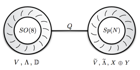
Figure 3: Depiction of the DGLSM defined by compactifying the 6D SCFT defined a $-4$ curve with $SO(8)$ gauge group on a Kähler surface. In two dimensions, we obtain a GLSM with gauge group $SO(8)\times Sp(N)$, and matter transforming in representations of the two gauge groups. Additionally, the GLSM sector is coupled to a collection of chiral and anti-chiral currents which are depicted by a thickened shell around each quiver node.

So far, we have kept the number of D3-branes as a free parameter. However, this is not really so, since we need to have a theory free of gauge anomalies. Now, we have seen that the chiral / anti-chiral bosons from reduction of the tensor multiplet do not contribute to the seven-brane gauge anomaly, so the only way for us to cancel the $SO(8)$ gauge anomaly will be through a combination of modes present in the quiver gauge theory.

Adding up the contribution from the $7-7$ strings and the $3-7$ strings, we have the $SO(8)$ anomaly:

$$k_{\text{tot}}(SO(8)) =k_{7-7}(SO(8))+k_{3-7}(SO(8))$$ (5.1)

$$=-\mathrm{Ind}(\mathrm{\mathbf{adj}}(SO(8)))\times(h^{0,0}-h^{0,1}+h^{0,2})+\mathrm{Ind}(\mathrm{\mathbf{fund}}(SO(8)))\times 2N.$$

Here, $\mathrm{Ind}(\mathrm{\mathbf{adj}}(G))$ is the index of the adjoint representation. In our normalization this is $2k$ for $SU(k)$ and $4k-4$ for $SO(2k)$. The index of the fundamental representation of $SO(2k)$ is then $2$. Setting $k_{\text{tot}}(SO(8))=0$, we can now solve for the total number of D3-branes:

$$N=\frac{\mathrm{Ind}(\mathrm{\mathbf{adj}}(SO(8)))}{2\mathrm{Ind}(\mathrm{\mathbf{fund}}(SO(8)))}\times\frac{P+3\chi}{12}=\frac{P+3\chi}{4}.$$ (5.2)

Note that in spite of appearances, this is always an integer since the holomorphic Euler characteristic is given by:

$$h^{0,0}-h^{0,1}+h^{0,2}=\chi(M_{4},\mathcal{O}_{M_{4}})=\frac{P+3\chi}{12}.$$ (5.3)

We can also see that our formula for the total number of D3-branes agrees with our general formula for the number of spacetime filling strings given in equation (4.51):

$$N_{\text{string}}=-k_{\text{inst}}+\frac{2h_{G}^{\vee}}{n}\chi(M_{4},\mathcal{O}_{M_{4}}),$$ (5.4)

where we set $k_{\text{inst}}=0$, $h_{G}^{\vee}=6$ and $n=4$.

Let us next verify that there is no gauge anomaly for the $Sp(N)$ sector. Recall that here, we have in the $3-3$ sector the contribution from a $(0,4)$ vector multiplet, i.e. we have two gauginos in the adjoint representation. Additionally, we have a $(0,4)$ hypermultiplet in the two-index symmetric representation, i.e. two CS multiplets. Finally, we have the $3-7$ sector which contributes eight $(0,4)$ half hypermultiplets in the fundamental representation, i.e., eight CS multiplets in the fundamental. Totalling up the contributions to the $Sp(N)$ anomaly, we have:

$$k_{\text{tot}}(Sp(N)) =k_{3-3}+k_{3-7}$$ (5.5)

$$=-2\times\mathrm{Ind}(\mathrm{\mathbf{adj}}(Sp(N)))+2\times\mathrm{Ind}(\mathrm{\mathbf{anti}}(Sp(N)))+8\times\mathrm{Ind}(\mathrm{\mathbf{fund}}(Sp(N)))$$

$$=-2(4N+4)+2(4N-4)+16=0.$$

Based on this, we conclude that we have indeed realized an anomaly free spectrum, as expected.

Let us now turn to the interaction terms of the theory. We primarily concentrate on the holomorphic terms, i.e. those associated with the superpotential and E-potential (for the Fermi multiplets). To this end, it is helpful to make manifest just the $(0,2)$ supersymmetry, so we write the $(0,4)$ half hypermultiplet in the bifundamental as a pair of CS multiplets $Q\oplus Q^{c}$ in conjugate representations of $U(4)\subset SO(8)$. To maintain a parallel description of the various interaction terms in the two sectors, we write all holomorphic data in terms of the associated E-potential for the Fermi multiplets where they appear. Due to the effective $(0,4)$ structure of the system, the resulting system is given by the E-potentials for the adjoint valued Fermi multiplets $\Lambda$ and $\widetilde{\Lambda}$:

$$E_{\Lambda} =\mathbb{D}\cdot T_{\text{SO(8)}}^{\text{adj}}\cdot\mathbb{D}+Q^{c}\cdot T_{\text{SO(8)}}^{\text{fund}}\cdot Q~{},$$ (5.6)

$$E_{\widetilde{\Lambda}} =X\cdot T_{\text{Sp(N)}}^{\text{symm}}\cdot Y+Q\cdot T_{\text{Sp(N)}}^{\text{fund}}\cdot Q^{c},$$ (5.7)

where the notation $A\cdot T_{G}\cdot B$ means that we take generators $T_{G}$ of the gauge group $G$ in the representation for $A$ and its conjugate representation $B$, and trace over all other symmetry indices.

Now, in addition to these couplings, we also have, from the reduction of the 6D Green-Schwarz term, an interaction term with bosonic content obtained from the reduction of line (4.41):

$$L_{2d}\supset\mu_{\mathrm{GS}}\underset{6D}{\int}B_{(2,0)}\wedge\text{Tr}(F_{2d}\wedge[\mathbb{D},\mathbb{D}])+B_{(2,0)}\wedge\text{Tr}(d_{A}\mathbb{D\wedge}d_{A}\mathbb{D})+c.c.$$ (5.8)

This sort of term is topological in 6D, and so we do not expect it to receive quantum corrections. Additionally, since it continues to play an important role in the low energy dynamics of the 2d system, we conclude that the R-charge assignments for the associated bosonic modes $B_{(2,0)}$ and $\mathbb{D}$ satisfy:

$$R\left(B_{(2,0)}\right)+2R(\mathbb{D)=}0.$$ (5.9)

But, unitarity ensures that all such R-charges must also be non-negative. Tracing through the rest of the relations in lines (5.6) and (5.7), we see that the R-charge assignments in this case all remain at their free-field values:

$$R(\mathbb{D)=}R(Q^{c})=R(Q)=R(X)=R(Y)=0.$$ (5.10)

Moreover, the R-charge assignments for the left-moving chiral bosons are protected since they are associated with symmetry currents. This also extends to all fermionic superpartners; each right–moving fermion in a chiral multiplet has R-charge $-1$. Additionally, based on the structure of the interactions, we see that all of the left–handed Weyl fermions in Fermi multiplets have R-charge $-1$.

So, as we expected from the 6D analysis, there appear to be no emergent $U(1)$ flavor symmetries which could mix with a candidate R-symmetry. Said differently, once we compute the anomaly polynomial, we will also be able to extract the IR R-symmetry without appealing to $c$-extremization.

5.1.1 Anomaly Polynomial

We now turn to the calculation of the 2d anomaly polynomial for this system:

$$I_{2d}=\frac{k_{RR}}{2}c_{1}(R_{2d,R})^{2}-\frac{k_{\text{grav}}}{24}p_{1}(TZ).$$ (5.11)

Where:

$$k_{RR}=\text{Tr}(\gamma_{3}R_{2d,R}R_{2d,R})\text{ \ \ and \ \ }k_{\text{grav}}=\text{Tr}(\gamma_{3}).$$ (5.12)

Since we are at weak coupling, and all R-charge assignments are fixed by the couplings of the model, it suffices to carefully count the various degrees of freedom in the system.

We begin with the calculation of $k_{RR}$. This includes the sectors associated with our GLSMs, as well as the contribution from the reduction of the anti-chiral two-form, i.e., we obtain additional chiral bosons, as well as additional vector multiplets from reduction on one-cycles. Finally, we also need to include the coupling between the chiral bosons and the background R-symmetry field strength, i.e., the corresponding 2d Green-Schwarz term.

Consider, then, the various contributions to $k_{RR}$. We have, in the obvious notation:

$$k_{RR}=k_{RR}^{7-7}+k_{RR}^{3-3}+k_{RR}^{3-7}+k_{RR}^{\text{Tensor}}+k_{RR}^{\text{GS}},$$ (5.13)

where the last term is due to the fact that there is a direct coupling between the chiral bosons and the $U(1)$ R-symmetry. Let us discuss each of these terms. First, from the $7-7$ strings, we have:

$$k_{RR}^{7-7}=\dim SO(8)\times\left(-h^{0,0}+h^{0,1}-h^{0,2}\right)=-28\times\left(\frac{P+3\chi}{12}\right).$$ (5.14)

Next, from the $3-3$ strings, we have:

$$k_{RR}^{3-3}=-2\times\dim Sp(N)\times(R_{\widetilde{\Lambda}})^{2}+2\times\mathrm{\dim}(\mathbf{anti}(Sp(N)))\times(R_{X}-1)^{2}=-4N.$$ (5.15)

From the $3-7$ strings, we have:

$$k_{RR}^{3-7}=8\times\mathrm{\dim}(\mathbf{fund}(Sp(N)))\times(R_{Q}-1)^{2}=16N.$$ (5.16)

Consider next the contribution from the reduction of the tensor multiplet fields. Here, we have both fermionic partners of the complex chiral bosons, $h^{2,0}+1$, all with R-charge $+1$, and gauginos for the $h^{1,0}$ modes obtained from taking one leg of the $B$-field on $M_{4}$ and one in the spacetime. The net contribution from these fermions to the anomaly is:

$$k_{RR}^{\text{Tensor}}=(h^{0,0}-h^{1,0}+h^{2,0})=\left(\frac{P+3\chi}{12}\right).$$ (5.17)

Finally, we turn to the contribution from the reduction of the Green-Schwarz term, i.e., terms associated with the exchange of the anti-chiral bosons. Now, in 6D, the relevant interaction term is:

$$L_{6D}\supset-n\int_{6D}B\wedge X,$$ (5.18)

where for the $SO(8)$ SNHC, we have:

$$X=\frac{1}{4}\text{Tr}F^{2}+\frac{6}{4}\left(c_{2}(R)+\frac{p_{1}(T)}{12}\right).$$ (5.19)

This yields the Green-Schwarz contribution to the 6D anomaly polynomial:

$$I_{6D}\supset\frac{4}{2}X^{2}\text{.}$$ (5.20)

A similar term will be present in the 2d anomaly polynomial, i.e., for the reducible contribution $c_{1}(R_{2d,R})^{2}$. To extract the form of this contribution to the 2d anomaly polynomial, we need to track the coupling of the chiral bosons to the relevant field strengths. Now, since we are integrating characteristic classes (of holomorphic vector bundles), we see that only the chiral bosons proportional to $(1,1)$ forms will actually contribute. Note there is at least one such contribution, since we have the Kähler class of the manifold itself. Observe, however, that this coupling does not involve the Pontryagin class at all. What this means is that it is not correct to simply integrate $X^{2}$ over $M_{4}$ to extract the contribution to $c_{1}(R_{2d,R})^{2}$. Indeed, part of the point of our analysis in this section has been to see how the 6D Green-Schwarz terms break up into separate contributions in the 2d effective theory.

Instead, we must only include those terms directly associated with the coupling of the 2d chiral bosons. In practical terms, this simply means we make the substitution $X\rightarrow X_{\text{eff}}$ compatible with the twist on $M_{4}$:

$$X_{\text{eff}}=-\frac{6}{4}c_{1}(R_{2d,R})c_{1}(K_{M_{4}}),$$ (5.21)

so that the contribution to the 2d anomaly polynomial is:

$$I_{2d}\supset\frac{4}{2}\int_{M_{4}}X_{\text{eff}}^{2}=\frac{9}{2}\times(P+2\chi)\times c_{1}(R_{2d,R})^{2}.$$ (5.22)

So in other words, the contribution to $k_{RR}$ is then:

$$k_{RR}^{\text{GS}}=9(P+2\chi).$$ (5.23)

We can now add up all of the contributions to $k_{RR}$, and we find:

$$k_{RR}=\frac{3}{4}\left(13P+27\chi\right),$$ (5.24)

which agrees with the general expression we presented in equation (2.48) from direct dimensional reduction of the 6D anomaly polynomial!

Consider next the contribution to $k_{\text{grav}}$. In this case there is no contribution from a Green-Schwarz term, as the $p_{1}(T)$ term is irreducible. Again, we split up the various contributions as:

$$k_{\text{grav}}=k_{\text{grav}}^{7-7}+k_{\text{grav}}^{3-3}+k_{\text{grav}}^{3-7}+k_{\text{grav}}^{\text{Tensor}}.$$ (5.25)

where the contributions from the GLSM sector are the same as for $k_{RR}$:

$$k_{\text{grav}}^{7-7} =\dim SO(8)\times(-h^{0,0}+h^{0,1}-h^{0,2})=-28\left(\frac{P+3\chi}{12}\right).$$ (5.26)

$$k_{\text{grav}}^{3-3} =-2\times\dim Sp(N)+2\times\mathrm{\dim}(\mathbf{anti}(Sp(N)))=-4N$$ (5.27)

$$k_{\text{grav}}^{3-7} =8\times\mathrm{\dim}(\mathbf{fund}(Sp(N)))=16N.$$ (5.28)

For the reduction of the anti-chiral two-form, we need to include the contributions from the fermionic superpartners, as well as the chiral bosons. The fermionic contribution to the gravitational anomaly is the same as what we already calculated for $k_{RR}$:

$$k_{\text{grav}}^{\text{Tensor,}F}=h^{0,0}-h^{1,0}+h^{2,0}=\left(\frac{P+3\chi}{12}\right).$$ (5.29)

Additionally, we have $2h^{2,0}+2$ right-moving chiral bosons, and $h^{1,1}$ left-moving chiral bosons. The difference between these two sectors contributions as the signature of the manifold:

$$k_{\text{grav}}^{\text{Tensor,}B}=b_{2}^{+}-b_{2}^{-}=\frac{P}{3}.$$ (5.30)

So in other words, the net contribution from reduction of the anti-chiral two-form to the gravitational anomaly is:

$$k_{\text{grav}}^{\text{Tensor}}=\left(\frac{5P+3\chi}{12}\right).$$ (5.31)

The net contribution to the gravitation anomaly is thus:

$$k_{\text{grav}}=\frac{13P+27\chi}{12},$$ (5.32)

which agrees with equation (2.47), which we obtained by direct dimensional reduction of the $-4$ curve SNHC!

An interesting feature of this case is that the ratio of $k_{RR}$ and $k_{\text{grav}}$ does not depend on the details of the four-manifold:

$$\frac{k_{RR}}{k_{\text{grav}}}=9.$$ (5.33)

5.2 Simple NHCs

The simplifying feature of the $-4$ curve theory is that we essentially had a standard GLSM coupled to a collection of chiral / anti-chiral bosons. In this sense, the whole theory is just a DGLSM. We now turn to the other simple NHCs where we do not a priori expect the spacetime filling strings to admit a description in terms of a GLSM. We can, however, still apply the general logic used in our analysis of the $SO(8)$ theory to calculate the resulting anomaly polynomial.

For the simple NHC  defined by a $-n$ curve, we have a simply laced gauge group $G$ which comes from a seven-brane on $\mathbb{R}^{1,1}\times M_{4}\times\mathbb{P}^{1}$. Additionally, we now have some number of spacetime filling strings which coupled to the seven-brane. Finally, we also have the contribution from the reduction of the tensor multiplet.

To see that spacetime filling strings are really necessary, consider just the GLSM sector from the seven-branes. The gauge anomaly for the gauge group $G$ is:

$$k_{7-7}(G)=-\mathrm{Ind}(\mathrm{\mathbf{adj}}(G))\times(h^{0,0}-h^{0,1}+h^{0,2})=-\mathrm{Ind}(\mathrm{\mathbf{adj}}(G))\left(\frac{P+3\chi}{12}\right).$$ (5.34)

The chiral bosons cannot contribute to anomaly cancellation, because this is a non-abelian gauge group factor. So, we must assume the presence of additional spacetime filling strings. Note that in weakly coupled terms, we need to add some number of CS multiplets to cancel the anomaly. This means in particular that we expect to cancel the anomaly with supersymmetric matter multiplets when $P+3\chi>0$.

Now, we can actually fix the total number of such strings using the structure of the anomaly polynomial for these 2d effective theories. This has recently been calculated in references [43, 44, 45], and in Appendix B we verify this by directly dimensionally reducing on a $\mathbb{P}^{1}$ the 4d $\mathcal{N}=2$ SCFTs (using the values of the anomalies obtained in references [98, 99, 100, 101]) that we obtain the same result. For our purposes, the presentation for the anomaly polynomial of $N$ spacetime filling strings in flat space given in reference [45] is most convenient. Focussing on just the symmetries which survive in compactifying on a Kähler surface, we have:

$$I_{\text{string}}=N\times\left(\frac{n}{4}\text{Tr}_{G}F^{2}-h_{G}^{\vee}\left(c_{2}(R)+\frac{1}{12}p_{1}(TZ)\right)\right)\text{,}$$ (5.35)

where in the above, we have introduced an overall relative minus sign between the gauge field strength term and the background R-symmetry and tangent bundle contributions. As we remarked before, this is due to the chirality conventions for our system, which as we shall shortly verify, led to a self-consistent prescription for supersymmetric anomaly cancellation.

Now, in our case where we can only activate a contribution from the 2d $U(1)$ R-symmetry and the background metric in two dimensions, the relevant expression is given by:

$$I_{\text{string}}=N\times\left(\frac{n}{4}\text{Tr}_{G}F^{2}-h_{G}^{\vee}\left(-c_{1}(R_{2d,R})^{2}+\frac{1}{12}p_{1}(TZ)\right)\right).$$ (5.36)

Returning to equation (5.34), we see that the total gauge anomaly is:

$$k_{\text{tot}}(G)=k_{7-7}(G)+k_{\text{string}}(G)=-\mathrm{Ind}(\mathrm{\mathbf{adj}}(G))\left(\frac{P+3\chi}{12}\right)+N\times n,$$ (5.37)

so the number of strings is fixed as:

$$N=\mathrm{Ind}(\mathrm{\mathbf{adj}}(G))\times\frac{1}{n}\times\left(\frac{P+3\chi}{12}\right).$$ (5.38)

Reassuringly, this agrees with our answer from the previous subsection in the special case $G=SO(8)$, where $\mathrm{Ind}(\mathrm{\mathbf{adj}}(G))=12$ and $n=4$. We can also repackage this formula using the fact that for all of the simply laced simple algebras (i.e. the gauge groups of the simple NHCs), $\mathrm{Ind}(\mathrm{\mathbf{adj}}(G))=2h_{G}^{\vee}$. So, we indeed recover the formula of equation (4.51):

$$N=\frac{2h_{G}^{\vee}}{n}\times\left(\frac{P+3\chi}{12}\right).$$ (5.39)

Now, in spite of the fact that we do not have a Lagrangian description for these spacetime filling strings, we can use the geometric picture to argue that there are (at least in the UV) no additional flavor symmetries. Assuming the absence of emergent abelian symmetries in the infrared, this means in particular that we can fix the R-charge assignments of fields in terms of UV data. Much as in our discussion of the weakly coupled model, we deduce that the R-charges of the GLSM fields are frozen to their free field values. Similar considerations hold for the chiral bosons of the system.

5.2.1 Anomaly Polynomial

Let us now turn to the calculation of the 2d anomaly polynomial. In this case, we again see no evidence for additional abelian flavor symmetries. Thus, our task reduces to calculating the coefficients in:

$$I_{2d}=\frac{k_{RR}}{2}c_{1}(R_{2d,R})^{2}-\frac{k_{\text{grav}}}{24}p_{1}(TZ),$$ (5.40)

where:

$$k_{RR}=\text{Tr}(\gamma_{3}R_{2d,R}R_{2d,R})\text{ \ \ and \ \ }k_{\text{grav}}=\text{Tr}(\gamma_{3}).$$ (5.41)

Now that we are at strong coupling, it will be more challenging to make detailed checks of the proposal. However, we can still rely on anomalies as a way to track this data. From this perspective, the main subtlety is to ensure that we fix our chirality convention so that all anomalies are cancelled with supersymmetric multiplets.

We begin with the calculation of $k_{RR}$. This includes the sectors associated with our GLSM, the spacetime filling strings, as well as the contribution from the reduction of the anti-chiral two-form, i.e., we obtain additional chiral bosons, as well as additional vector multiplets from reduction on one-cycles. Finally, we also need to include the coupling between the chiral bosons and the background R-symmetry field strength, i.e., the corresponding 2d Green-Schwarz term.

Consider, then, the various contributions to $k_{RR}$:

$$k_{RR}=k_{RR}^{7-7}+k_{RR}^{\text{strings}}+k_{RR}^{\text{Tensor}}+k_{RR}^{\text{GS}},$$ (5.42)

where the last term is due to the fact that there is a direct coupling between the chiral bosons and the $U(1)$ R-symmetry. Let us discuss each of these terms. First, from the $7-7$ strings, we have:

$$k_{RR}^{7-7}=d_{G}\times\left(-h^{0,0}+h^{0,1}-h^{0,2}\right)=-d_{G}\times\left(\frac{P+3\chi}{12}\right),$$ (5.43)

where $d_{G}$ is the dimension of the gauge group $G$.

Next, from the spacetime filling strings, we have the contribution:

$$k_{RR}^{\text{strings}}=2N\times h_{G}^{\vee}=\frac{4\left(h_{G}^{\vee}\right)^{2}}{n}\times\left(\frac{P+3\chi}{12}\right).$$ (5.44)

Observe in particular that for $P+3\chi>0$ this is a positive quantity, i.e., it is what we would get from summing up the contribution from CS, rather than Fermi multiplets, or (if supersymmetry had been broken) anti-CS multiplets.

The contribution from $k_{RR}^{\text{Tensor}}$ is the same as what we already found for the $SO(8)$ model:

$$k_{RR}^{\text{Tensor}}=(h^{0,0}-h^{1,0}+h^{2,0})=\left(\frac{P+3\chi}{12}\right).$$ (5.45)

Finally, there is the contribution from the Green-Schwarz term in two dimensions. Using the same analysis presented near line (5.18), we see that now, $X_{\text{eff}}$ is given by:

$$X_{\text{eff}}=-\frac{h_{G}^{\vee}}{n}c_{1}(R_{2d,R})c_{1}(K_{M_{4}}),$$ (5.46)

so that the contribution to the 2d anomaly polynomial is:

$$I_{2d}\supset\frac{n}{2}\int_{M_{4}}X_{\text{eff}}^{2}=\frac{\left(h_{G}^{\vee}\right)^{2}}{2n}\times(P+2\chi)\times c_{1}(R_{2d,R})^{2}.$$ (5.47)

So in other words, the contribution to $k_{RR}$ is then:

$$k_{RR}^{\text{GS}}=\frac{\left(h_{G}^{\vee}\right)^{2}}{n}(P+2\chi).$$ (5.48)

The sum total of all these contributions is therefore:

$$k_{RR} =-d_{G}\times\left(\frac{P+3\chi}{12}\right)+\frac{4\left(h_{G}^{\vee}\right)^{2}}{n}\times\left(\frac{P+3\chi}{12}\right)+\left(\frac{P+3\chi}{12}\right)+\frac{\left(h_{G}^{\vee}\right)^{2}}{n}(P+2\chi)$$ (5.49)

$$=(1-d_{G})\times\left(\frac{P+3\chi}{12}\right)+\frac{\left(h_{G}^{\vee}\right)^{2}}{3n}\times\left(4P+9\chi\right),$$ (5.50)

which agrees with equation (2.48), i.e., our formula obtained from dimensional reduction of the 6D SCFT anomaly polynomial!

Consider next the contributions to the gravitational anomaly. Just as in the $SO(8)$ example, there is no Green-Schwarz term as the $p_{1}(T)$ term is irreducible. We must, however, properly take into account the contributions from the chiral bosons. Again, we split up the various contributions as:

$$k_{\text{grav}}=k_{\text{grav}}^{7-7}+k_{\text{grav}}^{\text{strings}}+k_{\text{grav}}^{\text{Tensor}},$$ (5.51)

where:

$$k_{\text{grav}}^{7-7} =d_{G}\times(-h^{0,0}+h^{0,1}-h^{0,2})=-d_{G}\left(\frac{P+3\chi}{12}\right)$$ (5.52)

$$k_{\text{grav}}^{\text{strings}} =2h_{G}^{\vee}N=\frac{4\left(h_{G}^{\vee}\right)^{2}}{n}\times\left(\frac{P+3\chi}{12}\right)$$ (5.53)

$$k_{\text{grav}}^{\text{Tensor}} =\left(\frac{5P+3\chi}{12}\right),$$ (5.54)

which by inspection of equation (2.47) yields precisely the same answer as obtained from dimensional reduction of the 6D SCFT answer!

We can also compute the ratio $k_{RR}/k_{\text{grav}}$, which in the general case, does depend on the four-manifold:

$$\frac{k_{RR}}{k_{\text{grav}}}=\frac{n(d_{G}-1)(P+3\chi)-4\left(h_{G}^{\vee}\right)^{2}(4P+9\chi)}{n(d_{G}-1)(P+3\chi)-4\left(h_{G}^{\vee}\right)^{2}(P+3\chi)-4nP}.$$ (5.55)

Indeed, it appears to be a special property of just the $-4$ curve theory that all dependence on $P$ and $\chi$ vanishes. It would be quite interesting to understand this better.

5.3 Four-Manifold Constraints

In our analysis of anomalies, we left the general choice of four-manifold arbitrary. Of course, experience from higher-dimensional examples suggests that the particular choice will impact whether we realize a supersymmetric 2d theory at all.

As an example, the relative supersymmetries preserved by our DGLSM and our spacetime filling strings may be misaligned, thus leading to a non-supersymmetric matter spectrum. This depends on both the background curvatures of the four-manifold in question, as well as the choice of background flux from the seven-branes. Here, we focus on the case considered in the rest of the paper, i.e., where the flux of the seven-brane is trivial.

Returning to the weakly coupled $SO(8)$ model, we see that to cancel the $SO(8)$ gauge anomalies, it was necessary to add additional CS multiplets. The total number of such CS multiplets is:

$$N_{Q}\propto\frac{P+3\chi}{12},$$ (5.56)

where the constant of proportionality is positive. So, to have a supersymmetric matter spectrum we require:

$$\frac{P+3\chi}{12}>0,$$ (5.57)

a condition which is not always satisfied by a four-manifold.

Let us give some examples of both types. It is helpful to recall that the quantity we are considering is also given by the holomorphic Euler characteristic:

$$\frac{P(M_{4})+3\chi(M_{4})}{12}=\chi(M_{4},\mathcal{O}_{M_{4}})=1-h^{0,1}+h^{0,2}.$$ (5.58)

First of all, for all the del Pezzo surfaces $dP_{k}$ we have:

$$\frac{P(dP_{k})+3\chi(dP_{k})}{12}=1,$$ (5.59)

while for a K3 surface we have:

$$\frac{P(K3)+3\chi(K3)}{12}=2.$$ (5.60)

An additional class of examples comes from taking a Cartesian product of two Riemann surfaces $M_{4}=\Sigma_{1}\times\Sigma_{2}$:

$$\frac{P(\Sigma_{1}\times\Sigma_{2})+3\chi(\Sigma_{1}\times\Sigma_{2})}{12}=1-(g_{1}+g_{2})+g_{1}g_{2},$$ (5.61)

where $g_{i}$ is the genus of $\Sigma_{i}$. So, we see that if both $g_{1}=g_{2}=0$, this is positive, and it is non-negative if $g_{i}\geq 1$ for both $i$. In the case where one factor is a $\mathbb{P}^{1}$ and the other factor is a genus $g>1$ Riemann surface, we see that $\chi(M_{4},\mathcal{O}_{M_{4}})<0$, so in this case we do not realize a supersymmetric matter spectrum. More broadly, one can consider activating non-trivial background fluxes. This can lead to non-trivial bound states between the seven-brane and spacetime filling strings. A related way to preserve supersymmetry is to introduce defects, i.e. poles for some operators in the internal directions. We leave the analysis of these more general possibilities for future work.

Based on our discussion above, we conclude that for suitable four-manifolds, we realize a supersymmetric matter spectrum. A more subtle question has to do with whether the resulting infrared dynamics will support a supersymmetric vacuum. One way to partially address this is to calculate the Witten index and various examples of elliptic genera. As far as we are aware, this has not been carried out for any DGLSMs, and only for some examples of compactifications of $(2,0)$ theories (see e.g. [12]) so we leave this task for future work.

Though we have mainly focussed on theories with a single tensor multiplet, an alternative way to provide evidence for the existence of such fixed points for 6D SCFTs with a holographic dual (see e.g. [24, 15, 16, 25]) is to consider the resulting compactification on a four-manifold. Some examples along these lines have been worked out in references [48, 49, 50, 51, 52]), where one finds that for a four-manifold of negative curvature, there is a reduction from an $AdS_{7}$ solution to an $AdS_{3}$ solution. This is in line with the constraint $P+3\chi>0$ we have observed. Note also that this condition is somewhat weaker than what is required to get a weakly coupled gravity dual. Indeed, we expect that compactification on a del Pezzo surface or a K3 surface should also yield a sensible 2d conformal fixed point. The holographic dual of this case is likely to be a theory with higher spins in the bulk, which would be quite interesting to study further.

6 Conclusions

Compactifications of higher-dimensional SCFTs provide a general template for understanding many non-trivial aspects of lower-dimensional quantum systems. In this paper we have considered compactifications of 6D SCFTs on four-manifolds, using the higher-dimensional string theory description as a tool in the study of the resulting 2d effective field theories. In particular, we have argued that the resulting theory can also be understood by studying compactification on the tensor branch, where we obtain a dynamic GLSM, that is, a GLSM in which some parameters and couplings have been promoted to chiral / anti-chiral modes, and which is in turn typically coupled to a theory of spacetime filling effective strings. We have provided general evidence for this physical picture, by calculating, for example, the anomaly polynomial of this DGLSM, finding perfect agreement with the answer expected from compactification of the 6D SCFT. Turning the discussion around, we have also used the 6D (and ultimately stringy) perspective to shed light on the dynamics of DGLSMs. In the remainder of this section we discuss some avenues of future investigation.

One of the key simplifications we made in our analysis is to focus on the simple NHCs. It would be quite interesting to extend this to all of the NHCs, and to combine this with an analysis of compactification of the E-string theory on a four-manifold. This would provide a class of tools to systematically study more general compactifications of 6D SCFTs using the classification results of [14, 19].

There has recently been much study of other compactifications of 6D SCFTs, and in particular the case of the resulting 4d effective theories. It is tempting to combine this thread with the present one to develop a generalized 2d / 4d correspondence perhaps along the lines of reference [102]. Indeed, we have seen that some aspects of these 2d theories are remarkably tractable, and moreover, that the internal dynamics of these systems are often governed by a quasi-topological field theory coupled to various defects. In that context, another item of interest would be the calculation of the elliptic genera for our 2d effective theories.

Another natural avenue of investigation involves the study of various defects / punctures in these theories. Now, in contrast to the case of compactifications to four dimensions, the defects here will now be associated with complex curves, leading to a rather rich generalization of the purely algebraic data present for 4d theories.

The theories we have focussed on in this work are particularly simple because they have a single tensor multiplet. It is natural to also consider the opposite limit, i.e. where we take particular 6D SCFTs with a weakly coupled holographic dual. Compactifications of these systems on a negative curvature surface lead to $AdS_{3}$ vacua. It would be quite interesting to use the present perspective to extract further information about the resulting 2d CFTs thus obtained.

Finally, one of the original motivations for this work was to study a particularly tractable class of examples in which the moduli present in F-theory compactified on an elliptically fibered Calabi-Yau fivefold can be systematically decoupled (see in particular [54]). Having developed further tools to study such systems, it would be exciting to return to this more ambitious class of questions, and their application to questions in the cosmology of super-critical strings.

Appendix A Reduction of 6D Free Fields

This Appendix presents the detailed reduction of $(1,0)$ six dimensional superfields to two dimensions. While the main focus lies on the tensor multiplet, we also dimensionally reduce the vector- and hypermultiplet to provide a consistency check.

Before we discuss the actual dimensional reduction, let us review our superspace conventions. The superspace coordinates are $(x^{M},\theta^{\alpha s})$ where $x^{M}$ are the coordinates of the 6D spacetime and the Grassmann coordinates $\theta^{\alpha s}$ represent a symplectic Majorana-Weyl spinor. Spinor indices $\alpha,\,\beta,\,\dots$ parameterize the fundamental/anti-fundamental of $SO(5,1)\sim SU^{*}(4)$. We use the convention that $\psi^{\alpha}_{R}$ is right-handed chiral and $(\psi_{L})_{\alpha}$ has the opposite chirality. To avoid a redundancy in the notation, we either write $\psi_{R}$ or $\psi^{\alpha}$ and the same for left-handed spinors. Further, indices $s,\,t\,\dots$ represent the $Sp(1)\sim SU(2)$ $R$-symmetry. They are raised and lowered by totally antisymmetric $\Omega_{st}$, e.g. $\psi_{s}=\Omega_{st}\psi^{t}$ and $\psi^{s}=\Omega^{st}\psi_{t}$ with $\Omega^{su}\Omega_{ut}=\delta^{s}_{t}$. In most cases, we go to the explicit basis $s=(1,\,2)$ with $\Omega_{12}=-1$ and $\Omega^{12}=1$. Finally, there is complex conjugation which acts on pseudo-real symplectic Majorana-Weyl spinors as $\overline{\psi^{\alpha}_{s}}=\psi^{s\alpha}=\Omega^{st}\psi^{\alpha}_{t}$.

The 6D superspace derivatives

$$D_{\alpha}^{s}=\frac{\partial}{\partial\theta^{\alpha}_{s}}-i\theta^{s\beta}\partial_{\alpha\beta}$$ (A.1)

anti-commute with the supercharges

$$Q^{s}_{\alpha}=\frac{\partial}{\partial\theta^{\alpha}_{s}}+i\theta^{s\beta}\partial_{\alpha\beta}~{},$$ (A.2)

and they give rise to the algebra

$$\{D_{\alpha}^{s},D_{\beta}^{t}\}=-2i\Omega^{st}\partial_{\alpha\beta}\,,$$ (A.3)

while for the supercharges

$$\{Q_{\alpha}^{s},Q_{\beta}^{t}\}=2i\Omega^{st}\partial_{\alpha\beta}$$ (A.4)

holds. We use the abbreviation $\partial_{\alpha\beta}=\gamma_{\alpha\beta}^{M}\partial_{M}$ for partial derivatives contracted with an antisymmetric representation of the $\Gamma$-matrix sub-block $\gamma^{M}_{\alpha\beta}$. The full $8\times 8$ matrices have the form

$$\Gamma^{M}\Psi=\begin{pmatrix}0&\gamma^{M}_{\alpha\beta}\\ (\tilde{\gamma}^{M})^{\alpha\beta}&0\end{pmatrix}\begin{pmatrix}\psi_{\beta}\\ \psi^{\beta}\end{pmatrix}\,,\quad\tilde{\gamma}_{M}^{\alpha\beta}=\frac{1}{2}\epsilon^{\alpha\beta\sigma\delta}(\gamma_{M})_{\sigma\delta}\,.$$ (A.5)

Using this definition, we further find

$$\Gamma^{MN}\Psi=\begin{pmatrix}(\gamma^{MN})_{\alpha}{}^{\beta}&0\\ 0&(\tilde{\gamma}^{MN})^{\alpha}{}_{\beta}\end{pmatrix}\begin{pmatrix}\psi_{\beta}\\ \psi^{\beta}\end{pmatrix}$$ (A.6)

with

$$(\gamma^{MN})_{\alpha}{}^{\beta}=(\gamma^{[M}\tilde{\gamma}^{N]})_{\alpha}{}^{\beta}\quad\text{and}\quad(\tilde{\gamma}^{MN})^{\alpha}{}_{\beta}=-(\gamma^{MN})_{\beta}{}^{\alpha}\,.$$ (A.7)

In six dimensions the chirality operator is defined by

$$\Gamma_{7}=-\Gamma^{0}\Gamma^{1}\Gamma^{2}\Gamma^{3}\Gamma^{4}\Gamma^{5}\,.$$ (A.8)

Finally, there is the completeness relation

$$(\gamma^{MN})_{\alpha}{}^{\beta}(\gamma_{MN})_{\delta}{}^{\sigma}=2\delta_{\alpha}^{\beta}\delta_{\delta}^{\sigma}-8\delta^{\sigma}_{\alpha}\delta^{\beta}_{\delta}$$ (A.9)

that is quite useful for several calculations.

Reduction on Kähler Surface

In order to reduce the six dimensional theory on a Kähler surface $M_{4}$, we first split the coordinates according to $x^{M}=(y^{+},\,y^{-},\,z^{i},\,\overline{z}^{\bar{i}})$. The first two directions are identified with the external $\mathbb{R}^{1,1}$, while $M_{4}$ has the complex coordinated $z^{1}$, $z^{2}$. Further, we fix the metric

$$(ds)^{2}=-4dy^{+}dy^{-}\quad\text{or}\quad g_{+-}=-2\,,\quad g^{+-}=-\frac{1}{2}$$ (A.10)

of the external Minkowski space. On $M_{4}$ the only non-vanishing metric components are $g_{i\bar{j}}$.

In 6D, the covariantly constant spinor representing the parameter of supersymmetry transformations is denotes as $\eta^{s\alpha}$. It has the opposite chirality of the supercharge $Q_{\alpha}^{s}$. We use it to fix the + direction of the external coordinate system by requiring

$$\eta^{s\alpha}\gamma^{M}_{\alpha\beta}\eta^{t\beta}\partial_{M}=\Omega^{st}\partial_{+}\,.$$ (A.11)

For the following calculations, we introduce a left-handed counterpart of $\eta^{s\alpha}$ defined as:

$$\eta^{s}_{\alpha}=\gamma^{+}_{\alpha\beta}\eta^{s\beta}\,,$$ (A.12)

which immediately gives rise to $\eta^{s\alpha}\eta^{t}_{\alpha}=\Omega^{st}$. In addition to (A.12), we further obtain the relations

$$\tilde{\gamma}^{-\beta\alpha}\eta^{s}_{\alpha}=-\eta^{s}_{\beta}\,,\quad\gamma^{-}_{\beta\alpha}\eta^{s\alpha}=0\quad\text{and}\quad\tilde{\gamma}^{+\beta\alpha}\eta^{s}_{\alpha}=0$$ (A.13)

by requiring a consistent inner product for $\eta^{s\alpha}$.

In the spinor representation, the generator of the $\mathfrak{u}(1)_{M_{4}}$, which arises after decomposing the holonomy group $U(2)_{M_{4}}$ of $M_{4}$ into $SU(2)\times U(1)_{M_{4}}$, reads

$$J_{M_{4}}=-\frac{i}{4}\omega_{MN}\Gamma^{MN}$$ (A.14)

where

$$\omega_{MN}=\frac{i}{2}\Big{(}\eta^{1\beta}(\gamma_{MN})_{\beta}{}^{\alpha}\eta^{2}_{\alpha}+\eta^{2\beta}(\gamma_{MN})_{\beta}{}^{\alpha}\eta^{1}_{\alpha}\Big{)}$$ (A.15)

By construction this choice of $\omega_{MN}$, results in $\mathfrak{u}(1)_{M_{4}}$ charges $-1$/$+1$ for $\eta^{1\alpha}$/$\eta^{2\alpha}$. This can be checked by applying the completeness relation (A.9). Further, we denote the generator of the $\mathfrak{u}(1)_{R}$ cartan subalgebra of the $SU(2)$ $R$-symmetry as $J_{R}$. Taking into account the branching $\mathbf{2}\rightarrow+1\oplus-1$ of the fundamental in which $\eta^{s\alpha}$ transforms, we obtain the charges

$$J_{R}\eta^{1\alpha}=\eta^{1\alpha}\quad\text{and}\quad J_{R}\eta^{2\alpha}=-\eta^{2\alpha}\,.$$ (A.16)

The generator of the $U(1)_{\mathrm{diag}}$ which can be embedded $U(1)_{M_{4}}\times U(1)_{R}$ is $J_{\mathrm{diag}}=J_{M_{4}}+J_{R}$. Combining now the action of $J_{M_{4}}$ and $J_{R}$, we discussed so far, it is obvious that

$$J_{\mathrm{diag}}\eta^{s\alpha}=0$$ (A.17)

holds. Thus, we indeed can identify $\eta^{s\alpha}$ with a covariant constant spinor on $M_{4}$. As a convenient crosscheck, we note that this spinor has perspective negative chirality

$$\Gamma_{3,2d}=\Gamma^{0}\Gamma^{1}=\Gamma^{-}\Gamma^{+}-\Gamma^{+}\Gamma^{-}\,,$$ (A.18)

e.g. $\Gamma_{3,2d}\eta=-\eta$, from a 2d perspective. This is equivalent to spin +1/2. The corresponding conserved supercharges have the opposite chirality and spin.

We now use $\eta^{s\alpha}$ and its left-handed counterpart to construct the arbitrary 6D spinors:

$$\psi^{1}_{\alpha} =\Big{(}\frac{1}{4}\psi_{ij}\gamma^{ij}+\frac{1}{\sqrt{2}}\psi_{i}\gamma^{-i}+\psi\delta\Big{)}{}_{\alpha}{}^{\beta}\eta^{1}_{\beta} \psi^{2}_{\alpha} =\Big{(}\frac{1}{4}\overline{\psi}{}_{\bar{i}\bar{j}}\gamma^{\bar{i}\bar{j}}+\frac{1}{\sqrt{2}}\overline{\psi}{}_{\bar{i}}\gamma^{-\bar{i}}+\overline{\psi}\delta\Big{)}{}_{\alpha}{}^{\beta}\eta^{2}_{\beta}$$ (A.19)

$$\psi^{1\alpha} =\Big{(}\frac{1}{4}\psi_{ij}\gamma^{ij}+\frac{1}{\sqrt{2}}\psi_{i}\gamma^{+i}+\psi\delta\Big{)}{}_{\beta}{}^{\alpha}\eta^{1\beta} \psi^{2\alpha} =\Big{(}\frac{1}{4}\overline{\psi}{}_{\bar{i}\bar{j}}\gamma^{\bar{i}\bar{j}}+\frac{1}{\sqrt{2}}\overline{\psi}{}_{\bar{i}}\gamma^{+\bar{i}}+\overline{\psi}{}\delta\Big{)}{}_{\beta}{}^{\alpha}\eta^{2\beta}$$ (A.20)

out of differential forms on the Kähler surface $M_{4}$. These expression are explicit realizations of the branching rules

$$(\mathbf{4},\mathbf{2})\rightarrow (-1/2,\mathbf{1},2)\oplus(+1/2,\mathbf{2},+1)\oplus(-1/2,\mathbf{2},0)\oplus$$

$$(-1/2,1,-2)\oplus(+1/2,2,-1)\oplus(-1/2,1,0)$$ (A.21)

$$(\overline{\mathbf{4}},\mathbf{2})\rightarrow (+1/2,\mathbf{1},2)\oplus(-1/2,\mathbf{2},+1)\oplus(+1/2,\mathbf{2},0)\oplus$$

$$(+1/2,1,-2)\oplus(-1/2,2,-1)\oplus(+1/2,1,0)$$ (A.22)

from $\mathfrak{so}(5,1)\times\mathfrak{su}(2)_{R_{6}D}$ to $\mathfrak{so}(1,1)\times\mathfrak{su}(2)_{L}\times\mathfrak{u}(1)_{\mathrm{diag}}$. These equations provide an isomorphism between spinors in six dimensions and holomorphic/anti-holomorphic differential forms on $M_{4}$. We choose the normalization such that

$$\psi^{1\alpha}\phi^{2}_{\alpha} =\psi\overline{\phi}{}+\psi_{i}\overline{\phi}{}^{i}-\frac{1}{2}\psi_{ij}\overline{\phi}{}^{ij}$$

$$\psi^{2\alpha}\phi^{1}_{\alpha} =-\phi\overline{\psi}-\phi_{i}\overline{\psi}{}^{i}+\frac{1}{2}\phi_{ij}\overline{\psi}{}^{ij}=-\overline{\psi^{1\alpha}\phi^{2}_{\alpha}}$$ (A.23)

reproduces the natural pairing of $(p,q)$-forms applied to polyforms. To see how this works, consider the polyforms $\Psi=\psi_{(0,0)}+\psi_{(1,0)}+\psi_{(2,0)}$ and $\Phi$. We now write the pairing (A.23) as

$$\psi^{1\alpha}\phi^{2}_{\alpha}=(\Psi,\Phi)=(\psi_{(0,0)},\phi_{(0,0)})+(\psi_{(1,0)},\phi_{(1,0)})-(\psi_{(2,0)},\phi_{(2,0)})\,.$$ (A.24)

By remembering that the pairing in this equation utilizes the Hodge-star on $M_{4}$, we finally obtain

$$(\Psi,\Phi)\frac{\omega^{2}}{2}=\left.\sigma(\Psi)\wedge*\overline{\Phi}\right|_{\mathrm{top}}\,.$$ (A.25)

Here $\sigma$ is required to obtain the right sign for the two-form part in (A.24). It is defined as $\sigma(\psi)=(-1)^{(n-1)n/2}$ for a form $\psi$ of degree $n$.

As a first application of the presented spinor decomposition, we reduce the 6D superspace derivatives

$$D^{2}_{\alpha}=\frac{\partial}{\theta^{1\alpha}}-i\theta^{2\beta}\partial_{\alpha\beta}\quad\text{and}\quad D^{1}_{\alpha}=-\frac{\partial}{\theta^{2\alpha}}-i\theta^{1\beta}\partial_{\alpha\beta}\,.$$ (A.26)

to the $(0,2)$ superspace derivative

$$\mathbf{D}_{+} =\eta^{1\alpha}D^{2}_{\alpha}=\frac{\partial}{\partial\theta^{+}}-i\overline{\theta}{}^{+}\partial_{+}-i\sqrt{2}\overline{\theta}{}^{i}\partial_{i}\quad\text{and}$$

$$\overline{\mathbf{D}}_{+} =\eta^{2\alpha}D^{1}_{\alpha}=-\frac{\partial}{\partial\overline{\theta}{}^{+}}+i\theta^{+}\partial_{+}+i\sqrt{2}\theta^{\bar{i}}\partial_{\bar{i}}$$ (A.27)

in 2d by contraction with $\eta^{1\alpha}$ or $\eta^{2\alpha}$, respectively. In doing the calculation, we decompose the Grassmann coordinates $\theta^{s\alpha}$ in the same way as $\psi^{s\alpha}$ in (A.20). In order to decompose the partial derivative $\partial_{\alpha\beta}$, we further need the branching

$$\psi^{2\alpha}\gamma^{M}_{\alpha\beta}\phi^{1\beta}\lambda_{M}= -\overline{\psi}(\phi\lambda_{+}-\sqrt{2}\phi^{\bar{i}}\lambda_{\bar{i}})-\overline{\psi}^{i}(\sqrt{2}\phi\lambda_{i}+\sqrt{2}\phi_{ji}\lambda^{j}-\phi_{i}\lambda_{-})$$

$$+\frac{1}{2}\overline{\psi}{}^{ij}(\phi_{ij}\lambda_{+}+2\sqrt{2}\phi_{i}\lambda_{j})$$ (A.28)

of a vector, say $\lambda_{M}$. Again, this decomposition is compatible with the corresponding branching

$$(\mathbf{6},\mathbf{1})\rightarrow(-1,\mathbf{1},0)\oplus(+1,\mathbf{1},0)\oplus(0,\mathbf{2},+1)\oplus(0,\mathbf{2},-1)=\lambda_{+}\oplus\lambda_{-}\oplus\lambda_{(1,0)}\oplus\lambda_{(0,1)}$$ (A.29)

of $\mathfrak{so}(5,1)\times\mathfrak{su}(2)_{R_{6}D}\supset\mathfrak{so}(1,1)\times\mathfrak{su}(2)_{L}\times\mathfrak{u}(1)_{\mathrm{diag}}$. We here explicitly write the spinor index for the Grassmann variables $\theta^{+}$ and $\overline{\theta}{}^{+}$ in 2d to be compatible with the standard conventions. Except for the last term, (A.27) looks exactly like the $(0,2)$ derivatives given in [103]. In order to get rid of this term, we perform the coordinate transformation

$$\tilde{x}^{M}=\begin{pmatrix}x^{+}&x^{-}&x^{i}+i\sqrt{2}\,\theta^{+}\overline{\theta}{}^{i}&x^{\bar{i}}+i\sqrt{2}\,\overline{\theta}{}^{+}\theta^{\bar{i}}\end{pmatrix}\,.$$ (A.30)

The reduction of the supercharges to two dimensions works in the same way as for $D^{s}_{\alpha}$.

Vector multiplet

As a consistency check of the compactification procedure on a Kähler manifold $M_{4}$ presented in the last subsection, we apply it to the 6D vector multiplet. It is fully determined in terms of the gauge potential $\mathcal{A}_{\alpha\beta}$ of the covariant derivative

$$\mathcal{D}_{\alpha}^{s}=D_{\alpha}^{s}+i\mathcal{A}_{\alpha}^{s}$$ (A.31)

and contains a vector $A_{M}$, a right-handed symplectic Majorana-Weyl fermion $\lambda^{s\alpha}$ and an auxiliary field $Y^{st}$ in the adjoint of $SU(2)$. Our starting point is the real superfield

$$\mathcal{A}_{\alpha\beta}=A_{\alpha\beta}-2(\theta^{2\gamma}\lambda^{1\delta}-\theta^{1\gamma}\lambda^{2\delta})\epsilon_{\gamma\delta\alpha\beta}+\dots\,.$$ (A.32)

In order to identify the $(0,2)$ superfield resulting after the compactification, we take a closer look at the components

$$\mathcal{A}_{-}=\tilde{\gamma}^{\alpha\beta}_{-}\mathcal{A}_{\alpha\beta}=V+\overline{\theta}{}^{ij}\overline{\Lambda}{}_{ij}+\theta^{\bar{i}\bar{j}}\Lambda{}_{\bar{i}\bar{j}}+\dots\quad\text{and}\quad\mathcal{A}_{\bar{i}}=\tilde{\gamma}^{\alpha\beta}_{\bar{i}}\mathcal{A}_{\alpha\beta}=\mathds{A}_{\bar{i}}+\dots$$ (A.33)

with the corresponding superfields

$$V =A_{-}-2\overline{\theta}{}^{+}\lambda-2\theta^{+}\overline{\lambda}+\dots$$ (A.34)

$$\mathds{A}_{\bar{i}} =A_{\bar{i}}+2\sqrt{2}\theta^{+}\lambda_{\bar{i}}+\dots$$ (A.35)

$$\Lambda_{\bar{i}\bar{j}} =\lambda_{\bar{i}\bar{j}}+\dots$$ (A.36)

in two dimensions. These are exactly the superfields we studied in [54]. The gaugino $\lambda$ has negative chirality and therewith spin 1/2 (in our conventions it is a left–mover). All superfields transform in bundle $\mathcal{E}$ which combines the adjoint action of the gauge algebra and diffeomorphisms of the Kähler surface $M_{4}$. The latter are not dynamic. However, they have to be taken into account when counting fermionic zero modes weighted by the chirality. This zero mode count is given by the index $\chi(M_{4},\mathcal{E})$ which reduces to $\chi(M_{4},T^{\ast})$ for vanishing gauge field flux on $M_{4}$.

Hypermultiplet

A hypermultiplet is captured by the on-shell superfield $\mathcal{Q}^{s}$ transforming in the fundamental of the $SU(2)$ $R$-symmetry. Further, it has to satisfy the superspace constraint

$$\mathcal{D}^{(s}_{\alpha}\mathcal{Q}^{t)}=0\,,$$ (A.37)

where $\mathcal{D}^{s}_{\alpha}$ is the gauge covariant superspace derivative which fulfills the relation

$$\{\mathcal{D}_{\alpha}^{s},\mathcal{D}_{\beta}^{t}\}=-2i\Omega^{st}D_{\alpha\beta}\,.$$ (A.38)

It contains a complex scalar $q^{s}$ in the fundamental of $SU(2)$ and a left-handed Weyl-fermion $\chi_{\alpha}$.

To obtain the 2d superfield after the reduction, we start from the expansion

$$\mathcal{Q}^{s}=q^{s}+\theta^{s\alpha}\chi_{\alpha}+\dots$$ (A.39)

of the 6D superfield and express the Weyl-fermion in terms of antiholomorphic differential forms on the Kähler surface $M_{4}$. This gives rise to the expansion

$$\chi_{\alpha}=\Big{(}\frac{1}{4}\chi_{\bar{i}\bar{j}}\gamma^{\bar{i}\bar{j}}+\frac{1}{\sqrt{2}}\chi_{-\bar{i}}\gamma^{-\bar{i}}+\chi\delta\Big{)}{}_{\alpha}{}^{\beta}\eta^{2}_{\beta}\,.$$ (A.40)

Calculating the term $\theta^{2\alpha}\chi_{\alpha}$ requires to introduce the $(2,0)$ form

$$\mathbb{O}_{ij}=\frac{1}{2}\eta^{2\alpha}(\gamma_{ij})_{\alpha}{}^{\beta}\eta^{2}_{\beta}\quad\text{and its complex conjugate}\quad\overline{\mathbb{O}}_{\bar{i}\bar{j}}=\frac{1}{2}\eta^{1\alpha}(\gamma_{\bar{i}\bar{j}})_{\alpha}{}^{\beta}\eta^{1}_{\beta}\,.$$ (A.41)

The normalization chosen here gives rise to

$$(\mathbb{O},\mathbb{O})=\frac{1}{2}\mathbb{O}_{ij}\overline{\mathbb{O}}^{ij}=-1$$ (A.42)

Using $\mathbb{O}$, we find

$$\theta^{2\alpha}\chi_{\alpha}=\Big{(}\frac{1}{2}\overline{\theta}{}_{\bar{i}\bar{j}}\overline{\chi}{}+\overline{\theta}{}_{\bar{i}}\overline{\chi}{}_{\bar{j}}+\frac{1}{2}\overline{\theta}\,\overline{\chi}{}_{\bar{i}\bar{j}}\Big{)}\mathbb{O}^{\bar{i}\bar{j}}$$ (A.43)

and finally

$$\mathcal{Q}^{1}=Q^{1}+\theta^{\bar{i}}\Psi_{\bar{i}}+\dots\quad\text{and}\quad\mathcal{Q}^{2}=Q^{2}+\overline{\theta}{}_{\bar{i}}\Psi_{\bar{j}}\mathbb{O}^{\bar{i}\bar{j}}+\dots$$ (A.44)

with the $(0,2)$ superfields

$$Q^{1} =q^{1}+\theta^{+}\chi+\dots \Psi_{\bar{i}}=\chi_{\bar{i}}+\dots$$ (A.45)

$$Q^{2} =q^{2}+\frac{1}{2}\overline{\theta}{}^{+}\chi_{\bar{i}\bar{j}}\mathbb{O}^{\bar{i}\bar{j}}+\dots\,.$$ (A.46)

where $Q^{1}$ is chiral and $Q^{2}$ is antichiral. The bundle assignments for these superfields are

$$Q^{1}\in K_{M_{4}}^{1/2}\otimes\mathcal{R}_{1}\otimes\mathcal{R}_{2}^{\vee}\,,\quad Q^{2}\in K_{M_{4}}^{-1/2}\otimes\mathcal{R}_{1}\otimes\mathcal{R}_{2}^{\vee}\quad\text{and}\quad\Psi_{-\bar{i}}\in\Omega^{(0,1)}(K^{1/2}\otimes\mathcal{R}_{1}\otimes\mathcal{R}_{2}^{\vee})\,,$$ (A.47)

if we assume that $q^{s}$ transforms in the bifundamental $\mathcal{R}_{1}\otimes\mathcal{R}_{2}^{\vee}$. The square root of the canonical bundle $K^{1/2}$ in the bundle assignments is a consequence of the topological twist. In general, a superfield with charge $q$ under $J_{R}$ transforms in $K^{q/2}$. To make contact with the bundle assignments introduced in reference [54], we apply Serre duality to $Q^{2}$ resulting in

$$(Q^{2})^{c}\in K_{M_{4}}^{1/2}\otimes\mathcal{R}_{1}^{\vee}\otimes\mathcal{R}_{2}$$ (A.48)

and suppress the $SU(2)$ $R$-symmetry indices. Zero modes are counted by the corresponding cohomology classes. If we count the massless fermions weighted by their chirality, we obtain the index $\chi(M_{4},K_{M_{4}}^{1/2}\otimes\mathcal{R}_{1}\otimes\mathcal{R}_{2})$. This matches perfectly with the results in [54]. The SUSY transformation rules are given there.

Tensor multiplet

We implement the tensor multiplet as a real, on-shell superfield $\mathcal{T}$ which is constrained by

$$D^{(s}_{\alpha}D^{t)}_{\beta}\mathcal{T}=0\,.$$ (A.49)

It contains a real scalar $t_{6D}$, the left-handed symplectic Majorana-Weyl fermion $\xi^{s}_{\alpha}$ and the anti-self-dual 3-form flux $H^{(-)}_{MNL}$, here in bispinor representation $H_{\alpha\beta}=\gamma_{\alpha\beta}^{MNL}H^{(-)}_{MNL}$. As the multiplet is on-shell, these fields have to fulfill the equations of motion

$$\partial_{M}\partial^{M}t_{6D}=0\,,\quad\partial^{\alpha\beta}\xi^{+}_{\beta}=0\quad\text{and}\quad\partial^{\alpha\gamma}H_{\gamma\alpha}=0\,.$$ (A.50)

Remember that in six dimensions each 3-form can be decomposed into a self-dual and a anti-self-dual part

$$H_{MNL}=H^{(+)}_{MNL}+H^{(-)}_{MNL}\quad\text{with}\quad H^{(\pm)}_{MNL}=\frac{1}{2}(H_{MNL}\pm*H_{MNL})\,.$$ (A.51)

These two parts get mapped to spinor indices

$$H^{\alpha\beta}=H^{(+)}_{MNL}(\tilde{\gamma}^{MNL})^{\alpha\beta}\quad\text{and}\quad H_{\alpha\beta}=H^{(-)}_{MNL}\gamma^{MNL}_{\alpha\beta}\,.$$ (A.52)

Thus, we see that $H_{(\alpha\beta)}$ in the tensor multiplet’s equations of motion (A.50) represent the anti-self-dual $H^{(-)}$. Because we are interested in massless fields in two dimensions, we expand it using all $b_{2}$ elements of $H^{2}(S,\mathbb{R})$. They decompose into $\dot{\alpha}=1,\dots,b_{2}^{+}$ self-dual and $\alpha=1,\dots,b_{2}^{-}$ anti-self-dual two forms. Here, we use the same notation as in section 3. The splitting in self-dual and anti-self-dual cohomology representatives $\lambda_{\dot{\alpha}}$/$\lambda_{\alpha}$ give rise to the expansion

$$H^{(-)}=\partial_{+}\varphi_{L}^{\dot{\alpha}}(x^{+})\wedge\lambda_{\dot{\alpha}}+\partial_{-}\varphi_{R}^{\alpha}(x^{-})\wedge\lambda_{\alpha}\,.$$ (A.53)

Here the 2d scalars $\varphi_{L}^{\alpha}$/$\varphi_{R}^{\dot{\alpha}}$ have to be chiral/anti-chiral otherwise $H^{(-)}$ would violate the anti-self-duality constraint. Repeating this discussion for $H$ contributions with one or three legs in the internal space, we find that they have to vanish on-shell due to the self-duality constraint.

In order to obtain the $(0,2)$ multiplets in two dimensions, we again start from the superspace expansion

$$\mathcal{T}= t_{6D}-\theta^{2\alpha}\xi^{1}_{\alpha}+\theta^{1\alpha}\xi^{2}_{\alpha}+\theta^{2\alpha}\theta^{1\beta}(H_{\alpha\beta}-i\partial_{\alpha\beta}\phi)-i\theta^{2\alpha}\theta^{2\beta}\theta^{1\gamma}\partial_{\beta\gamma}\xi^{1}_{\alpha}+$$

$$i\theta^{2\alpha}\theta^{1\beta}\theta^{1\gamma}\partial_{\alpha\beta}\xi^{2}_{\gamma}-\frac{1}{2}\theta^{2\alpha}\theta^{2\beta}\theta^{1\gamma}\theta^{1\delta}\partial_{\alpha\gamma}\partial_{\beta\delta}\phi-i\theta^{2\alpha}\theta^{2\beta}\theta^{1\gamma}\theta^{1\delta}\partial_{\beta\delta}H_{\alpha\gamma}+\dots$$ (A.54)

which solves the constraint (A.49) on-shell. Going from the bispinor representation $H_{\alpha\beta}$ to the corresponding anti-self-dual 3-form, we obtain

$$\theta^{2\alpha}\gamma^{MNL}_{\alpha\beta}\theta^{1\beta}H^{(-)}_{MNL}= -\overline{\theta}(6\theta H_{+}{}_{\bar{i}}{}^{\bar{i}}-6\theta^{\bar{i}\bar{j}}H_{+\bar{i}\bar{j}})-12\overline{\theta}{}^{i}\theta^{\bar{j}}H_{-\bar{j}i}$$

$$+\frac{1}{2}\overline{\theta}{}^{ij}(12\theta H_{+ij}+12\theta_{ik}H_{+j}{}^{k})$$ (A.55)

and implement the branching

$$(\mathbf{10},\mathbf{1}) \rightarrow(+1,\mathbf{3},0)\oplus(-1,\mathbf{1},2)\oplus(-1,\mathbf{1},0)\oplus\xcancel{(0,\mathbf{2},1)}\oplus\xcancel{(0,\mathbf{2},-1)}$$

$$=H_{-i\bar{j}}\text{ with }H_{-i}{}^{i}=0\,\oplus H_{+ij}\oplus H_{+\bar{i}}{}^{\bar{i}}\oplus H_{+\bar{i}\bar{j}}\,.$$ (A.56)

from $\mathfrak{so}(5,1)\times\mathfrak{su}(2)_{6D,R}$ to $\mathfrak{so}(1,1)\times\mathfrak{su}(2)_{L}\times\mathfrak{u}(1)_{\mathrm{diag}}$. The last products of irreps do not contribute because they correspond to three-from fluxes with only one or all three legs in the internal directions. As we already explained, such configurations are ruled out on-shell by the equations of motion. Finally, one finds

$$\Phi=t_{L}+\operatorname{Re}\mathbb{\tau}_{R}-\overline{\theta}{}^{i}\Xi_{i}-\frac{1}{2}\overline{\theta}{}^{ij}\Xi_{ij}+12\theta^{\bar{i}}\overline{\theta}{}^{j}\mathcal{H}_{-\bar{i}j}+\dots+\text{c.c.}$$ (A.57)

which allows us to identify the $(0,2)$ multiplets

$$\operatorname{Re}\mathbb{\tau}_{R}(\tilde{x}^{M}) =t_{R}+\theta^{+}\overline{\xi}-\overline{\theta}{}^{+}\xi-6\overline{\theta}{}^{+}\theta^{+}H_{+\bar{i}}{}^{\bar{i}} \Xi_{i}(\tilde{x}^{M}) =\xi_{i}+i\overline{\theta}{}^{+}\theta^{+}\partial_{+}\xi_{i}$$

$$\Xi_{ij}(\tilde{x}^{M}) =\xi_{ij}+12\theta^{+}H_{+ij}+i\overline{\theta}{}^{+}\theta^{+}\partial_{+}\xi_{ij} \mathcal{H}_{-\bar{i}j}(\tilde{x}^{M}) =H_{-\bar{i}j}.$$ (A.58)

We split $t_{6D}=t_{L}+t_{R}$ into left- and right-moving parts, as explained in section 4. It is important that we use the coordinates $\tilde{x}^{M}$ which we introduce in (A.30) for these multiplets. For $x^{M}$ the results would not be conclusive because the 2d superspace derivatives do not have the standard form. In principle, we face the same problem for the vector and hypermultiplet in the last subsections. But there we only considered the leading components which are always free from obstructions.

Only the multiplet $\operatorname{Re}\mathbb{\tau}_{R}$ appears somewhat exotic. It is real and contains the right-moving part of the tensor multiplets scalar as leading contribution. Its highest component is a chiral boson $H_{+}$ which is proportional to the Kähler form $\omega$ on $M_{4}$. As we explained in section 4, it is, in fact, not mysterious: it is simply the real part of the corresponding CS multiplet. The Hodge number $2h^{2,0}$ counts the number of massless multiplets $\Xi_{ij}$ (weighted by 2 because they are complex, and we counting real degrees of freedom) and the $1$ corresponds to the real multiplet $\operatorname{Re}\mathbb{\tau}_{L}$. All $b_{2}^{(-)}$ anti-chiral bosons form singlets under supersymmetry and are captured by $\mathcal{H}_{-\bar{i}\bar{j}}$. Finally $\Xi_{i}$ hosts the two gauginos of the $U(1)^{2}$ abelian gauge theory arising from compactifying the 6D $B$-field with one leg in the internal and one leg in the external directions. Off-shell this multiplet also contains the corresponding field strength and an auxiliary field as bosonic degrees of freedom. On-shell all bosonic contributions vanish and we are left with the gauginos. From $\operatorname{Re}\mathbb{\tau}_{R}$ we can derive the abelian current multiplet

$$\Xi=\mathbf{D}_{+}\operatorname{Re}\mathbb{\tau}_{R}=\xi+i\theta^{+}(H_{+\bar{i}}{}^{\bar{i}}+\partial_{+}t_{L})-i\overline{\theta}{}^{+}\theta^{+}\partial_{+}\xi$$ (A.59)

which will be useful in deriving the superconformal current multiplet in the next subsection.

Finally we calculate the $(0,2)$ SUSY variation

$$\delta_{\epsilon}=\overline{\epsilon}{}^{+}\overline{Q}_{+}-\epsilon^{+}Q_{+}$$ (A.60)

of the real multiplet $\operatorname{Re}\mathbb{\tau}_{R}$. It gives rise to

$$\delta_{\epsilon}t_{R} =\overline{\epsilon}{}^{+}\xi_{+}-\epsilon^{+}\overline{\xi}{}_{+} \delta_{\epsilon}\xi_{+} =-\epsilon^{+}(6H_{+\bar{i}}{}^{\bar{i}}+i\partial_{+}t_{R})$$

$$H_{+\bar{i}}{}^{\bar{i}} =\frac{i}{6}(\epsilon^{+}\partial_{+}\overline{\xi}{}_{+}+\overline{\epsilon}{}^{+}\partial_{+}\xi{}_{+}) \delta_{\epsilon}\overline{\xi}{}_{+} =-\overline{\epsilon}{}^{+}(6H_{+\bar{i}}{}^{\bar{i}}-i\partial_{+}t_{R})$$ (A.61)

and is compatible with $t_{R}$ and $iH_{+\bar{i}}{}^{\bar{i}}$ being real.

Supercurrents for Tensor Multiplet

The chiral bosons arising from the reduction of the tensor multiplet make it difficult to write down an action for the $(0,2)$ multiplets discussed in the last subsection. But we still can explicitly calculate the energy momentum tensor of the two dimensional theory. To this end, we first consider the 6D real supercurrent

$$J=\frac{1}{2}\mathcal{T}^{2}\,.$$ (A.62)

It gives rise to the superfield

$$V^{st}_{\alpha\beta}=D^{(s}_{\alpha}D^{t)}_{\beta}J=v^{st}_{\alpha\beta}+\dots$$ (A.63)

which hosts the conserved $R$-symmetry current as its leading part $v^{12}_{\alpha\beta}$ [104]. We are interested in the component $V^{21}_{\alpha\beta}$. It is associated to the Cartan generator $J_{R}$ of $\mathfrak{su}(2)$ and thus the $R$-symmetry in 2d. The two antisymmetric spinor indices this multiplet carries can be mapped to a vector index

$$V^{12}_{M}=\tilde{\gamma}_{M}^{\alpha\beta}V^{12}_{\alpha\beta}=\tilde{\gamma}_{M}^{\alpha\beta}v^{12}_{\alpha\beta}+\dots\,.$$ (A.64)

In the $\mathbb{R}^{1,1}$ directions the leading components of this vector are:

$$V^{12}_{+} =\xi\overline{\xi}-\frac{1}{2}\xi_{ij}\overline{\xi}{}^{ij}+\dots$$ (A.65)

$$V^{12}_{-} =\xi_{i}\overline{\xi}{}^{i}.$$ (A.66)

These leading contributions are sufficient to figure out the full expression for $V^{12}_{M}$ in terms of the superfields we introduced in the last subsection. We obtain

$$V_{+}^{12}=\overline{D}{}^{+}\mathcal{T}D^{-}\mathcal{T}-\frac{1}{2}\Xi_{ij}\overline{\Xi}{}^{ij}=\Xi\overline{\Xi}-\frac{1}{2}\Xi_{ij}\overline{\Xi}{}^{ij}\quad\text{and}\quad V_{-}^{12}=-\Xi_{i}\overline{\Xi}^{i}~{},$$ (A.67)

where we have used (A.59). It is straightforward to check that these two superfields represent conserved currents in 2d, namely they fulfill $\partial_{-}V_{+}^{12}=\partial_{+}V_{-}^{12}=0$. The latter is a singlet, while the former is the superconformal current of a 2d SCFT. It has exactly the form one would expect from the $(0,2)$ Sugawara construction of chiral currents [105].

Appendix B Effective Strings from 4d $\mathcal{N}=2$ SCFTs

In this Appendix we provide further details on the spacetime filling strings which are a necessary ingredient in the construction of our 2d theories. In string theory terms, these effective strings arise from $N$ D3-branes wrapped on the collapsing $\mathbb{P}^{1}$ factor of $M_{4}\times\mathbb{P}^{1}$, the six-manifold wrapped by the seven-brane. Here, the $\mathbb{P}^{1}$ factor has self-intersection $-n$ in the base of an F-theory model.

Now, in the limit where the volume of the $\mathbb{P}^{1}$ is very large, we can approximate this system by the 4d theory defined by D3-branes probing a seven-brane with gauge group $G$. For the simple NHCs, this realizes 4d $\mathcal{N}=2$ superconformal field theories where the seven-branes contribute a flavor symmetry $G$. Various aspects of these theories have been studied for example in references [90, 91, 92, 93, 94, 95, 99, 100, 101, 106, 107, 108, 109, 110]. In what follows we will include the free hypermultiplet describing motion of the center of mass for the D3-branes inside the seven-brane.

In addition to the flavor symmetry localized on the seven-brane, we also have the geometric isometries associated with directions both inside the seven-brane, i.e., an $SO(4)_{\|}$ symmetry, and transverse to the seven-brane, i.e. $U(1)_{\bot}$. The R-symmetry of the 4d $\mathcal{N}=2$ SCFT is realized by $SU(2)_{R}\times U(1)_{\bot}$, where we use the isomorphism $SO(4)_{\|}\simeq SU(2)_{L}\times SU(2)_{R}/\mathbb{Z}_{2}$. The generator for the 4d $\mathcal{N}=1$ R-symmetry is given by the linear combination:

$$R_{\mathcal{N}=1}=\frac{1}{3}R_{\mathcal{N}=2}+\frac{2}{3}I^{(3)},$$ (B.1)

where $R_{\mathcal{N}=2}$ is the generator associated with $U(1)_{\bot}$ and $I^{(3)}$ is the generator of the Cartan subalgebra of $SU(2)_{R}$, with eigenvalues $\pm 1$ in the fundamental representation. For the theories in question, the usual central charges

$$a=\frac{3}{32}\left(3\mathrm{Tr}R_{\mathcal{N}=1}^{3}-\mathrm{Tr}R_{\mathcal{N}=1}\right)\ ,\qquad c=\frac{1}{32}\left(9\mathrm{Tr}R_{\mathcal{N}=1}^{3}-5\mathrm{Tr}R_{\mathcal{N}=1}\right)\ ,$$ (B.2)

reduce to:

$$a=\frac{1}{8}N^{2}n+\frac{1}{12}Nh_{G}^{\vee}\ ,\qquad c=\frac{1}{8}N^{2}n+\frac{1}{8}Nh_{G}^{\vee}\ .$$ (B.3)

Here, we include the contribution from the free hypermultiplet parameterizing the center of mass degree of freedom for the stack of D3-branes inside of the seven-branes.

The anomalies for these theories have been computed in references [7, 98, 99, 101, 107]. It is convenient to assemble these expressions into a single anomaly polynomial which depends on the background field strengths $F_{G}$, $F_{L}$, $F_{R}$, $F_{\bot}$, and $T$, the background tangent bundle:

$$I_{4d} =\frac{k_{\bot GG}}{4}\left(c_{1}(F_{\bot})\mathrm{Tr}F_{G}^{2}\right)+\frac{k_{\bot\bot\bot}}{6}\left(c_{1}(F_{\bot})^{3}\right)+\frac{k_{\bot TT}}{24}\left(c_{1}(F_{\bot})p_{1}(T)\right)$$ (B.4)

$$+\frac{k_{\bot LL}}{4}\left(c_{1}(F_{\bot})\mathrm{Tr}F_{L}^{2}\right)+\frac{k_{\bot RR}}{4}\left(c_{1}(F_{\bot})\mathrm{Tr}F_{R}^{2}\right).$$ (B.5)

where the explicit values are:

$$k_{\bot GG} =-Nn\text{, \ \ }k_{\bot\bot\bot}=-2Nh_{G}^{\vee}\text{, \ \ }k_{\bot TT}=2Nh_{G}^{\vee}\text{, \ \ }$$ (B.6)

$$k_{\bot LL} =-N\left(Nn-\frac{h_{G}^{\vee}}{3}\right)\text{, \ \ }k_{\bot RR}=N\left(Nn+\frac{h_{G}^{\vee}}{3}\right),$$ (B.7)

which are in turn obtained by evaluating the anomalies:

$$k_{\bot GG}\times\delta^{AB} =\text{Tr}(R_{\mathcal{N}=2}T^{A}T^{B})\text{, \ \ }k_{\bot\bot\bot}=\text{Tr}(R_{\mathcal{N}=2}^{3})\text{, \ \ }k_{\bot TT}=-\text{Tr}(R_{\mathcal{N}=2})\text{,}$$ (B.8)

$$k_{\bot LL}\times\delta^{ab} =\text{Tr}(R_{\mathcal{N}=2}I_{L}^{a}I_{L}^{b})\text{, \ \ }k_{\bot RR}\times\delta^{ab}=\text{Tr}(R_{\mathcal{N}=2}I_{R}^{a}I_{R}^{b})\text{,}$$ (B.9)

where in the above, we have introduced the Lie algebra generators $T^{A}$ for the flavor group $G$ and generators $I_{L}^{a}$ and $I_{R}^{b}$ for $SU(2)_{L}$ and $SU(2)_{R}$.

Next, consider the dimensional reduction of the 4d theory on a $\mathbb{P}^{1}$. In this case, the $SU(2)_{R}$ factor of $SO(4)_{\|}\simeq SU(2)_{L}\times SU(2)_{R}/\mathbb{Z}_{2}$ remains as a spectator, and we only use the abelian factor coming from the $U(1)_{\bot}$ factor of the 4d $\mathcal{N}=2$ SCFT. This is required in order to match to the symmetries preserved by the $\mathcal{N}=2$ SCFT. So, we introduce the specific decomposition:

$$R_{4d}^{\mathcal{N}=2}=R_{2d,R}\otimes K_{\mathbb{P}^{1}}^{1/2},$$ (B.10)

where $K_{\mathbb{P}^{1}}$ is the canonical bundle on $\mathbb{P}^{1}$. The overall twist is dictated by the same analysis presented, for example in reference [111]. The first Chern class splits up as:

$$c_{1}\left(F_{\bot}\right)=c_{1}(R_{2d,R})+\frac{1}{2}c_{1}(K_{\mathbb{P}^{1}})\ .$$ (B.11)

To obtain the anomaly polynomial of the 2d effective strings, we now integrate over the $\mathbb{P}^{1}$. To this end, we make the subsitutions $p_{1}(T)\rightarrow p_{1}(TZ)$, and use the fact that:

$$\int_{\mathbb{P}^{1}}c_{1}(K_{\mathbb{P}^{1}})=-2.$$ (B.12)

The 2d anomaly polynomial is then given by:

$$I_{2d} =\frac{Nn}{4}\mathrm{Tr}F_{G}^{2}+Nh_{G}^{\vee}\left(c_{1}(R_{2d,R})^{2}-\frac{1}{12}p_{1}(TZ)\right)$$ (B.13)

$$+\frac{N}{4}\left(Nn-\frac{h_{G}^{\vee}}{3}\right)\mathrm{Tr}F_{L}^{2}-\frac{N}{4}\left(Nn+\frac{h_{G}^{\vee}}{3}\right)\mathrm{Tr}F_{R}^{2}.$$ (B.14)

On a curved background where $F_{L}$ and $F_{R}$ are generically broken, this reduces to:

$$I_{2d}=\frac{Nn}{4}\mathrm{Tr}F_{G}^{2}+Nh_{G}^{\vee}\left(c_{1}(R_{2d,R})^{2}-\frac{1}{12}p_{1}(TZ)\right),$$ (B.15)

which is the expression used in section 5.

Weakly Coupled Example

To check that we have correctly fixed all normalizations, as well as all relative signs, it is helpful to return to a weakly coupled example where all contributions to the anomaly polynomial can be explicitly evaluated. Along these lines, we consider the 4d $\mathcal{N}=2$ SCFT defined by $SU(2)$ gauge theory with four flavors in the fundamental representation, and a decoupled free hypermultiplet. This is the special case $N=1$ and $n=4$. In terms of $\mathcal{N}=1$ multiplets, the matter content consists of four chiral multiplets $Q\oplus Q^{c}$, another pair of chiral multiplets $H\oplus H^{c}$, a chiral multiplet $\Phi$ in the adjoint representation of $SU(2)$, and a vector multiplet $V$. In this presentation, we have a manifest $U(4)$ flavor symmetry which enhances to $SO(8)$. In our normalization conventions for generators, the fermionic components of each multiplet (denoted by $\psi$) have charge assignments:

$$\begin{tabular}[c]{|c|c|c|c|c|c|}\hline\cr&$I_{L}^{(3)}$&$I_{R}^{(3)}$&$U(1)_{\bot}$&$U(4)$&$SU(2)_{D3}$\\ \hline\cr$\psi_{Q}$&$0$&$0$&$-1$&$\mathbf{4}$&$\mathbf{2}$\\ \hline\cr$\psi_{Q^{c}}$&$0$&$0$&$-1$&$\overline{\mathbf{4}}$&$\mathbf{2}$\\ \hline\cr$\psi_{H}$&$+1$&$0$&$-1$&$\mathbf{1}$&$\mathbf{1}$\\ \hline\cr$\psi_{H^{c}}$&$-1$&$0$&$-1$&$\mathbf{1}$&$\mathbf{1}$\\ \hline\cr$\psi_{\Phi}$&$0$&$-1$&$+1$&$\mathbf{1}$&$\mathbf{3}$\\ \hline\cr$\psi_{V}$&$0$&$+1$&$+1$&$\mathbf{1}$&$\mathbf{3}$\\ \hline\cr\end{tabular}.$$ (B.16)

Let us now verify that our formulae agree with the normalization conventions used in lines (B.6) and (B.7). In the obvious notation, we have:

$$k_{\bot GG} =k_{\bot GG}(\psi_{Q})+k_{\bot GG}(\psi_{Q^{c}})=-2-2=-4\text{,}$$ (B.17)

$$k_{\bot\bot\bot} =k_{\bot\bot\bot}(\psi_{Q})+k_{\bot\bot\bot}(\psi_{Q^{c}})+k_{\bot\bot\bot}(\psi_{H})+k_{\bot\bot\bot}(\psi_{H^{c}})+k_{\bot\bot\bot}(\psi_{\Phi})+k_{\bot\bot\bot}(\psi_{V})$$

$$=-8-8-1-1+3+3=-12,$$ (B.18)

$$k_{\bot TT} =k_{\bot TT}(\psi_{Q})+k_{\bot TT}(\psi_{Q^{c}})+k_{\bot TT}(\psi_{H})+k_{\bot TT}(\psi_{H^{c}})+k_{\bot TT}(\psi_{\Phi})+k_{\bot TT}(\psi_{V})$$

$$=+8+8+1+1-3-3=+12,$$ (B.19)

$$k_{\bot LL} =k_{\bot LL}(\psi_{H})+k_{\bot LL}(\psi_{H^{c}})=-1-1=-2\text{,}$$ (B.20)

$$k_{\bot RR} =k_{\bot RR}(\psi_{\Phi})+k_{\bot RR}(\psi_{V})=3+3=6\text{.}$$ (B.21)

Returning to lines (B.6) and (B.7) and plugging in $N=1$ and $n=4$, we obtain the same values.

References

- [1] E. Witten, “Some comments on string dynamics,” in Future perspectives in string theory. Proceedings, Conference, Strings’95, Los Angeles, USA, March 13-18, 1995. 1995. arXiv:hep-th/9507121.
- [2] A. Strominger, “Open P-Branes,” Phys. Lett. B383 (1996) 44–47, arXiv:hep-th/9512059.
- [3] N. Seiberg, “Nontrivial fixed points of the renormalization group in six-dimensions,” Phys. Lett. B390 (1997) 169–171, arXiv:hep-th/9609161.
- [4] C. Montonen and D. I. Olive, “Magnetic Monopoles as Gauge Particles?,” Phys. Lett. B72 (1977) 117–120.
- [5] C. Vafa, “Geometric Origin of Montonen-Olive Duality,” Adv. Theor. Math. Phys. 1 (1998) 158–166, arXiv:hep-th/9707131.
- [6] E. Witten, “Solutions of Four-Dimensional Field Theories via M-theory,” Nucl. Phys. B500 (1997) 3–42, arXiv:hep-th/9703166.
- [7] P. C. Argyres and N. Seiberg, “S-duality in Supersymmetric Gauge Theories,” JHEP 12 (2007) 088, arXiv:0711.0054 [hep-th].
- [8] D. Gaiotto, “ Dualities,” JHEP 08 (2012) 034, arXiv:0904.2715 [hep-th].
- [9] J. M. Maldacena, A. Strominger, and E. Witten, “Black Hole Entropy in M-theory,” JHEP 12 (1997) 002, arXiv:hep-th/9711053.
- [10] E. Witten, “Fivebranes and Knots,” arXiv:1101.3216 [hep-th].
- [11] T. Dimofte, D. Gaiotto, and S. Gukov, “Gauge Theories Labelled by Three-Manifolds,” Comm. Math. Phys. 325 (2014) 367–419, arXiv:1108.4389 [hep-th].
- [12] A. Gadde, S. Gukov, and P. Putrov, “Fivebranes and 4-manifolds,” arXiv:1306.4320 [hep-th].
- [13] S. Gukov, P. Putrov, and C. Vafa, “Fivebranes and 3-manifold homology,” arXiv:1602.05302 [hep-th].
- [14] J. J. Heckman, D. R. Morrison, and C. Vafa, “On the Classification of 6D SCFTs and Generalized ADE Orbifolds,” JHEP 05 (2014) 028, arXiv:1312.5746 [hep-th]. [Erratum: JHEP (2015) 017].
- [15] D. Gaiotto and A. Tomasiello, “Holography for (1,0) theories in six dimensions,” JHEP 12 (2014) 003, arXiv:1404.0711 [hep-th].
- [16] M. Del Zotto, J. J. Heckman, A. Tomasiello, and C. Vafa, “6d Conformal Matter,” JHEP 02 (2015) 054, arXiv:1407.6359 [hep-th].
- [17] J. J. Heckman, “More on the Matter of 6D SCFTs,” Phys. Lett. B747 (2015) 73–75, arXiv:1408.0006 [hep-th].
- [18] M. Del Zotto, J. J. Heckman, D. R. Morrison, and D. S. Park, “6D SCFTs and Gravity,” JHEP 06 (2015) 158, arXiv:1412.6526 [hep-th].
- [19] J. J. Heckman, D. R. Morrison, T. Rudelius, and C. Vafa, “Atomic Classification of 6D SCFTs,” Fortsch. Phys. 63 (2015) 468–530, arXiv:1502.05405 [hep-th].
- [20] L. Bhardwaj, “Classification of 6d gauge theories,” JHEP 11 (2015) 002, arXiv:1502.06594 [hep-th].
- [21] Y. Tachikawa, “Frozen,” arXiv:1508.06679 [hep-th].
- [22] A. Hanany and A. Zaffaroni, “Branes and six-dimensional supersymmetric theories,” Nucl. Phys. B529 (1998) 180–206, arXiv:hep-th/9712145.
- [23] L. Bhardwaj, M. Del Zotto, J. J. Heckman, D. R. Morrison, T. Rudelius, and C. Vafa, “F-theory and the Classification of Little Strings,” Phys. Rev. D93 no. 8, (2016) 086002, arXiv:1511.05565 [hep-th].
- [24] F. Apruzzi, M. Fazzi, D. Rosa, and A. Tomasiello, “All solutions of type II supergravity,” JHEP 04 (2014) 064, arXiv:1309.2949 [hep-th].
- [25] F. Apruzzi, M. Fazzi, A. Passias, A. Rota, and A. Tomasiello, “Six-Dimensional Superconformal Theories and their Compactifications from Type IIA Supergravity,” Phys. Rev. Lett. 115 no. 6, (2015) 061601, arXiv:1502.06616 [hep-th].
- [26] M. Del Zotto, J. J. Heckman, D. S. Park, and T. Rudelius, “On the Defect Group of a 6D SCFT,” arXiv:1503.04806 [hep-th].
- [27] D. Gaiotto and S. S. Razamat, “ theories of class ,” JHEP 07 (2015) 073, arXiv:1503.05159 [hep-th].
- [28] K. Ohmori, H. Shimizu, Y. Tachikawa, and K. Yonekura, “6d theories on and class S theories: Part I,” JHEP 07 (2015) 014, arXiv:1503.06217 [hep-th].
- [29] S. Franco, H. Hayashi, and A. Uranga, “Charting Class Territory,” Phys. Rev. D92 no. 4, (2015) 045004, arXiv:1504.05988 [hep-th].
- [30] M. Del Zotto, C. Vafa, and D. Xie, “Geometric engineering, mirror symmetry and ,” JHEP 11 (2015) 123, arXiv:1504.08348 [hep-th].
- [31] A. Hanany and K. Maruyoshi, “Chiral Theories of Class ,” JHEP 12 (2015) 080, arXiv:1505.05053 [hep-th].
- [32] M. Aganagic and N. Haouzi, “ADE Little String Theory on a Riemann Surface (and Triality),” arXiv:1506.04183 [hep-th].
- [33] K. Ohmori, H. Shimizu, Y. Tachikawa, and K. Yonekura, “6d theories on S1 /T2 and class S theories: Part II,” JHEP 12 (2015) 131, arXiv:1508.00915 [hep-th].
- [34] I. Coman, E. Pomoni, M. Taki, and F. Yagi, “Spectral curves of theories of class ,” arXiv:1512.06079 [hep-th].
- [35] D. R. Morrison and C. Vafa, “F-Theory and SCFTs in Four Dimensions,” arXiv:1604.03560 [hep-th].
- [36] J. J. Heckman, P. Jefferson, T. Rudelius, and C. Vafa, “Punctures for Theories of Class ,” arXiv:1609.01281 [hep-th].
- [37] M. B. Green and J. H. Schwarz, “Anomaly Cancellation in Supersymmetric D=10 Gauge Theory and Superstring Theory,” Phys. Lett. B149 (1984) 117–122.
- [38] M. B. Green, J. H. Schwarz, and P. C. West, “Anomaly Free Chiral Theories in Six-Dimensions,” Nucl. Phys. B254 (1985) 327–348.
- [39] A. Sagnotti, “A Note on the Green-Schwarz Mechanism in Open String Theories,” Phys. Lett. B294 (1992) 196–203, arXiv:hep-th/9210127.
- [40] V. Sadov, “Generalized Green-Schwarz mechanism in F theory,” Phys. Lett. B388 (1996) 45–50, arXiv:hep-th/9606008.
- [41] D. R. Morrison and W. Taylor, “Classifying bases for 6D F-theory models,” Central Eur. J. Phys. 10 (2012) 1072–1088, arXiv:1201.1943 [hep-th].
- [42] A. Gadde, B. Haghighat, J. Kim, S. Kim, G. Lockhart, and C. Vafa, “6d String Chains,” arXiv:1504.04614 [hep-th].
- [43] H.-C. Kim, S. Kim, and J. Park, “6d strings from new chiral gauge theories,” arXiv:1608.03919 [hep-th].
- [44] H. Shimizu and Y. Tachikawa, “Anomaly of strings of 6d theories,” arXiv:1608.05894 [hep-th].
- [45] M. Del Zotto and G. Lockhart, “On Exceptional Instanton Strings,” arXiv:1609.00310 [hep-th].
- [46] O. J. Ganor, “Compactification of Tensionless String Theories,” arXiv:hep-th/9607092.
- [47] B. Assel, S. Schafer-Nameki, and J.-M. Wong, “M5-branes on : Nahm’s Equations and 4d Topological Sigma-models,” arXiv:1604.03606 [hep-th].
- [48] J. P. Gauntlett, N. Kim, and D. Waldram, “M-Fivebranes Wrapped on Supersymmetric Cycles,” Phys. Rev. D63 (2001) 126001, arXiv:hep-th/0012195.
- [49] J. P. Gauntlett, O. A. P. Mac Conamhna, T. Mateos, and D. Waldram, “AdS spacetimes from wrapped M5 branes,” JHEP 11 (2006) 053, arXiv:hep-th/0605146.
- [50] P. Figueras, O. A. P. Mac Conamhna, and E. O Colgain, “Global geometry of the supersymmetric / correspondence in M-theory,” Phys. Rev. D76 (2007) 046007, arXiv:hep-th/0703275.
- [51] A. Passias, A. Rota, and A. Tomasiello, “Universal consistent truncation for 6d/7d gauge/gravity duals,” JHEP 10 (2015) 187, arXiv:1506.05462 [hep-th].
- [52] P. Karndumri and E. . Colgáin, “3D supergravity from wrapped M5-branes,” JHEP 03 (2016) 188, arXiv:1508.00963 [hep-th].
- [53] E. Witten, “Phase Transitions in M-theory and F-theory,” Nucl. Phys. B471 (1996) 195–216, arXiv:hep-th/9603150.
- [54] F. Apruzzi, F. Hassler, J. J. Heckman, and I. V. Melnikov, “UV Completions for Non-Critical Strings,” JHEP 07 (2016) 045, arXiv:1602.04221 [hep-th].
- [55] E. Witten, “Topological Quantum Field Theory,” Comm. Math. Phys. 117 (1988) 353.
- [56] G. Festuccia and N. Seiberg, “Rigid Supersymmetric Theories in Curved Superspace,” JHEP 06 (2011) 114, arXiv:1105.0689 [hep-th].
- [57] C. Klare, A. Tomasiello, and A. Zaffaroni, “Supersymmetry on Curved Spaces and Holography,” JHEP 08 (2012) 061, arXiv:1205.1062 [hep-th].
- [58] T. T. Dumitrescu, G. Festuccia, and N. Seiberg, “Exploring Curved Superspace,” JHEP 08 (2012) 141, arXiv:1205.1115 [hep-th].
- [59] K. Ohmori, H. Shimizu, and Y. Tachikawa, “Anomaly Polynomial of E-string Theories,” JHEP 08 (2014) 002, arXiv:1404.3887 [hep-th].
- [60] K. Ohmori, H. Shimizu, Y. Tachikawa, and K. Yonekura, “Anomaly Polynomial of General 6d SCFTs,” PTEP 2014 no. 10, (2014) 103B07, arXiv:1408.5572 [hep-th].
- [61] J. J. Heckman, D. R. Morrison, T. Rudelius, and C. Vafa, “Geometry of 6D RG Flows,” JHEP 09 (2015) 052, arXiv:1505.00009 [hep-th].
- [62] J. J. Heckman and T. Rudelius, “Evidence for C-theorems in 6D SCFTs,” JHEP 09 (2015) 218, arXiv:1506.06753 [hep-th].
- [63] J. J. Heckman, T. Rudelius, and A. Tomasiello, “6D RG Flows and Nilpotent Hierarchies,” JHEP 07 (2016) 082, arXiv:1601.04078 [hep-th].
- [64] F. Benini and N. Bobev, “Exact two-dimensional superconformal R-symmetry and c-extremization,” Phys. Rev. Lett. 110 no. 6, (2013) 061601, arXiv:1211.4030 [hep-th].
- [65] F. Benini and N. Bobev, “Two-dimensional SCFTs from wrapped branes and c-extremization,” JHEP 06 (2013) 005, arXiv:1302.4451 [hep-th].
- [66] J. Teschner, “Liouville theory revisited,” Class. Quant. Grav. 18 (2001) R153–R222, arXiv:hep-th/0104158 [hep-th].
- [67] E. Witten, “On the conformal field theory of the Higgs branch,” JHEP 07 (1997) 003, arXiv:hep-th/9707093 [hep-th].
- [68] J. A. Harvey, D. Kutasov, and S. Lee, “Comments on Quantum Higgs Vacua,” JHEP 07 (2015) 071, arXiv:1406.6000 [hep-th].
- [69] K. Hori and A. Kapustin, “Duality of the fermionic 2-D black hole and N=2 liouville theory as mirror symmetry,” JHEP 08 (2001) 045, arXiv:hep-th/0104202.
- [70] A. Adams, M. Ernebjerg, and J. M. Lapan, “Linear models for flux vacua,” Adv. Theor. Math. Phys. 12 no. 4, (2008) 817–852, arXiv:hep-th/0611084.
- [71] A. Adams, E. Dyer, and J. Lee, “GLSMs for non-Kähler Geometries,” JHEP 01 (2013) 044, arXiv:1206.5815 [hep-th].
- [72] C. Quigley, S. Sethi, and M. Stern, “Novel Branches of (0,2) Theories,” JHEP 09 (2012) 064, arXiv:1206.3228 [hep-th].
- [73] I. V. Melnikov, C. Quigley, S. Sethi, and M. Stern, “Target Spaces from Chiral Gauge Theories,” JHEP 02 (2013) 111, arXiv:1212.1212 [hep-th].
- [74] D. Israel and M. Sarkis, “New supersymmetric index of heterotic compactifications with torsion,” JHEP 12 (2015) 069, arXiv:1509.05704 [hep-th].
- [75] E. Witten, “Nonperturbative Superpotentials in String Theory,” Nucl. Phys. B474 (1996) 343–360, arXiv:hep-th/9604030.
- [76] O. J. Ganor, “A Note On Zeroes of Superpotentials in F-Theory,” Nucl. Phys. B499 (1997) 55–66, arXiv:hep-th/9612077.
- [77] J. J. Heckman, J. Marsano, N. Saulina, S. Schafer-Nameki, and C. Vafa, “Instantons and SUSY breaking in F-theory,” arXiv:0808.1286 [hep-th].
- [78] J. Marsano, N. Saulina, and S. Schafer-Nameki, “An Instanton Toolbox for F-Theory Model Building,” JHEP 01 (2010) 128, arXiv:0808.2450 [hep-th].
- [79] M. Cvetic, I. Garcia-Etxebarria, and R. Richter, “Branes and instantons intersecting at angles,” JHEP 01 (2010) 005, arXiv:0905.1694 [hep-th].
- [80] R. Donagi and M. Wijnholt, “MSW Instantons,” JHEP 06 (2013) 050, arXiv:1005.5391 [hep-th].
- [81] C. Beasley, J. J. Heckman, and C. Vafa, “GUTs and exceptional branes in F-theory - II: Experimental predictions,” JHEP 01 (2009) 059, arXiv:0806.0102 [hep-th].
- [82] C. Córdova, “Decoupling gravity in F-theory,” Adv. Theor. Math. Phys. 15 (2011) 689–740, arXiv:0910.2955 [hep-th].
- [83] J. J. Heckman and H. Verlinde, “Evidence for F(uzz) Theory,” JHEP 01 (2011) 044, arXiv:1005.3033 [hep-th].
- [84] S. Schafer-Nameki and T. Weigand, “F-theory and 2d (0,2) Theories,” arXiv:1601.02015 [hep-th].
- [85] C. Vafa and E. Witten, “A One-Loop Test of String Duality,” Nucl. Phys. B447 (1995) 261–270, arXiv:hep-th/9505053 [hep-th].
- [86] K. Dasgupta and S. Mukhi, “A Note on Low-Dimensional String Compactifications,” Phys. Lett. B398 (1997) 285–290, arXiv:hep-th/9612188.
- [87] S. Gukov, C. Vafa, and E. Witten, “CFT’s From Calabi-Yau Four-folds,” Nucl. Phys. B584 (2000) 69–108, arXiv:hep-th/9906070. [Erratum: Nucl. Phys.B608,477(2001)].
- [88] S. J. Gates, Jr., S. Gukov, and E. Witten, “Two Two-Dimensional Supergravity Theories from Calabi-Yau Four-Folds,” Nucl. Phys. B584 (2000) 109–148, arXiv:hep-th/0005120.
- [89] I. L. Buchbinder and N. G. Pletnev, “Construction of 6D Supersymmetric Field Models in Harmonic Superspace,” Nucl. Phys. B892 (2015) 21–48, arXiv:1411.1848 [hep-th].
- [90] J. A. Minahan and D. Nemeschansky, “An Superconformal Fixed Point with Global Symmetry,” Nucl. Phys. B482 (1996) 142–152, arXiv:hep-th/9608047 [hep-th].
- [91] J. A. Minahan and D. Nemeschansky, “Superconformal Fixed Points with Global Symmetry,” Nucl. Phys. B489 (1997) 24–46, arXiv:hep-th/9610076 [hep-th].
- [92] P. C. Argyres and M. R. Douglas, “New Phenomena in Supersymmetric Gauge Theory,” Nucl. Phys. B448 (1995) 93–126, arXiv:hep-th/9505062 [hep-th].
- [93] N. Seiberg and E. Witten, “Monopoles, Duality and Chiral Symmetry Breaking in Supersymmetric QCD,” Nucl. Phys. B431 (1994) 484–550, arXiv:hep-th/9408099.
- [94] A. Sen, “F theory and orientifolds,” Nucl. Phys. B475 (1996) 562–578, arXiv:hep-th/9605150 [hep-th].
- [95] T. Banks, M. R. Douglas, and N. Seiberg, “Probing -theory With Branes,” Phys. Lett. B387 (1996) 278–281, arXiv:hep-th/9605199 [hep-th].
- [96] K. Kodaira and D. C. Spencer, “On deformations of complex analytic structures. III. Stability theorems for complex structures,” Ann. of Math. (2) 71 (1960) 43–76.
- [97] N. Buchdahl, “On compact Kähler surfaces,” Ann. Inst. Fourier (Grenoble) 49 no. 1, (1999) vii, xi, 287–302.
- [98] Y.-K. E. Cheung, O. J. Ganor, and M. Krogh, “Correlators of the global symmetry currents of 4-D and 6-D superconformal theories,” Nucl. Phys. B523 (1998) 171–192, arXiv:hep-th/9710053 [hep-th].
- [99] O. Aharony and Y. Tachikawa, “A Holographic Computation of the Central Charges of , SCFTs,” JHEP 01 (2008) 037, arXiv:0711.4532 [hep-th].
- [100] P. C. Argyres and J. R. Wittig, “Infinite Coupling Duals of Gauge Theories and New Rank 1 Superconformal Field Theories,” JHEP 01 (2008) 074, arXiv:0712.2028 [hep-th].
- [101] A. D. Shapere and Y. Tachikawa, “Central Charges of Superconformal Field Theories in Four Dimensions,” JHEP 09 (2008) 109, arXiv:0804.1957 [hep-th].
- [102] L. F. Alday, D. Gaiotto, and Y. Tachikawa, “Liouville Correlation Functions from Four-dimensional Gauge Theories,” Lett. Math. Phys. 91 (2010) 167–197, arXiv:0906.3219 [hep-th].
- [103] E. Witten, “Phases of Theories in Two Dimensions,” Nucl. Phys. B403 (1993) 159–222, arXiv:hep-th/9301042.
- [104] P. S. Howe, G. Sierra, and P. K. Townsend, “Supersymmetry in Six-Dimensions,” Nucl. Phys. B221 (1983) 331–348.
- [105] C. M. Hull and B. J. Spence, “ Current Algebra and Coset Models,” Phys. Lett. B241 (1990) 357–364.
- [106] M. Noguchi, S. Terashima, and S.-K. Yang, “ Superconformal Field Theory with ADE Global Symmetry on a D3-brane Probe,” Nucl. Phys. B556 (1999) 115–151, arXiv:hep-th/9903215.
- [107] Y. Tachikawa and B. Wecht, “Explanation of the Central Charge Ratio 27/32 in Four-Dimensional Renormalization Group Flows between Superconformal Theories,” Phys. Rev. Lett. 103 (2009) 061601, arXiv:0906.0965 [hep-th].
- [108] J. J. Heckman and C. Vafa, “An Exceptional Sector for F-theory GUTs,” Phys. Rev. D83 (2011) 026006, arXiv:1006.5459 [hep-th].
- [109] J. J. Heckman, Y. Tachikawa, C. Vafa, and B. Wecht, “ SCFTs from Brane Monodromy,” JHEP 11 (2010) 132, arXiv:1009.0017 [hep-th].
- [110] M. Del Zotto, J. J. Heckman, P. Kumar, A. Malekian, and B. Wecht, “Kinetic Mixing at Strong Coupling,” arXiv:1608.06635 [hep-ph].
- [111] F. Benini, N. Bobev, and P. M. Crichigno, “Two-dimensional SCFTs from D3-branes,” JHEP 07 (2016) 020, arXiv:1511.09462 [hep-th].