SPARSE: A Subgrid Particle Averaged Reynolds Stress Equivalent Model: Testing with A Priori Closure

Abstract

A Lagrangian particle cloud model is proposed that accounts for the effects of Reynolds-averaged particle and turbulent stresses and the averaged carrier-phase velocity of the sub-particle-cloud scale on the averaged motion and velocity of the cloud. The SPARSE (Subgrid Particle Average Reynolds Stress Equivalent) model is based on a combination of a truncated Taylor expansion of a drag correction function and Reynolds averaging. It reduces the required number of computational parcels to trace a cloud of particles in Eulerian-Lagrangian methods for the simulation of particle-laden flow . Closure is performed in an a priori manner using a reference simulation where all particles in the cloud are traced individually with a point particle model. Comparison of a first-order model and SPARSE with the reference simulation in one-dimension shows that both the stress and the averaging of the carrier-phase velocity on the cloud subscale affect the averaged motion of the particle. A three-dimensional isotropic turbulence computation shows that only one computational parcel is sufficient to accurately trace a cloud of tens of thousand of particles.

1 Introduction

The Eulerian-Lagrangian (EL) model, introduced by Crowe at al. [1, 2], is one of the major approaches used to for computing the interaction of a large number of particles with a turbulent flow. In the EL model each particle is traced in its Lagrangian frame, i.e. the frame moving with the particle. Because particles are treated as volumeless mathematical points in the EL “point-particle” approach, the tracing of many particles becomes much more computationally efficient. With a point-particle assumption, the simulation of large number of particles in process-scale environments becomes feasible.

If the number of particles in a computation is prohibitively large, groups of physical particles are amalgamated into a single computational particle to further economize the computational cost. This type of method is also known as Cloud-In-Cell (CIC) [3]. In CIC methods, groups of particles are modeled as points and their motion is forced by the drag exerted on them by the fluid [4, 5, 6, 7]. The CIC method as conventionally implemented does not account for sub-particle cloud dynamics resulting from turbulent fluctuations or particle-particle interactions.

For the modeling of subgrid and/or sub-particle-cloud scales of turbulent carrier-phase flows, Large-Eddy Simulation is commonly employed. In LES, filtered Navier-Stokes equations resolve large turbulent structures, while dissipation of energy from the subgrid scales (SGS) is modeled. Commonly used SGS models include the classic Smagorinsky [8] and Dynamic Smagorinsky [9] models.

Similar to the modeling of SGS with eddy viscosity models in the carrier phase, SGS models are required for an accurate particle tracer [10, 11, 12, 13, 14]. To this end, models have been formulated with either a deterministic approach or stochastic modeling of subgrid scales. In the deterministic approach, the instantaneous velocities are reconstructed for use in particle equations through defiltering [15, 16, 17, 18, 19]. Shotorban and co-workers [15, 17, 19] employed Approximate Deconvolution (AD) [20] for defiltering. Deconvolution is a mathematical method to approximately reconstruct the instantaneous velocity through consecutively applying a filtering operation on the filtered velocities. The consecutive application of the filtering operator is a result of a series expansion for the deconvolution. Filtering, itself, is a convolution product of the instantaneous velocity and the filter kernel. Kuerten and Verman [16] employed a defiltering technique in which the filtering inversion is carried out in the Fourier space for the streamwise and spanwise directions while the inversion is approximated by a Taylor series for the cross-stream direction. Although defiltering is efficient to implement, it can only be carried out for the represented modes.

A Langevin type stochastic differential equation can be used to compute the evolution of particles when the carrier phase is simulated by LES [21, 15, 22]. A similar model was previously proposed for particles by Pozorski and Minier [23, 24] and Minier and Peirano [25] when the carrier phase is simulated by RANS. Shotorban and Mashayek [22] extended the application of the Langevin equation from a simple RANS framework [23, 24, 25] to a higher-resolution LES model by using the stochastic differential equation employed to solve LES equations through a Filtered Density Function approach [26]. A modified version of this model was proposed by Berrouk et al. [27] to account for crossing-trajectory effects.

While the modeling the effect of subgrid stresses on the dispersion of particles has been studied, the effect of sub-scale particle fluctuations under the computational particle assumptions of CIC has received much less attention. Several articles [28, 29, 30] have studied the inclusion of small-scale particle-fluid energy transfer in their turbulence models. However, these studies focus on the effect that the particles have on the fluid rather than the influence of individual modeled particles on the averaged computational particle dynamics.

In recent work, we have undertaken a multi-scaling modeling effort [31] in which macro-scale models such as the LES and CIC models are closed using results from full resolution meso-scale simulations that solve for the turbulence and flow over particles with moving boundaries. The general framework enables direct closure of averaging terms in a wide parameter space that otherwise would take a great range of challenging and meticolous experimentation to obtain emperical formulas. Within this framework, we have more freedom to develop macro-models, for example, for particle cloud dynamics.

This paper presents a model that accounts for sub-scale interphase velocity perturbations on computational particle dispersion patterns in a CIC framework. The model is general and is a good fit for a multi-scale framework. The drag forcing term in the Lagrangian governing equation for the particle momentum employs a correction factor for high Reynolds and Mach numbers. The particle drag correction factor is expanded using a Taylor expansion, which enables a simple Reynolds averaging of the governing equations to yield a second order perturbation term. These higher order terms are deemed ”Reynolds Stress Equivalent” terms, which capture the effects of meso-scale interphase velocity perturbations. We therefore refer to the model as Subgrid Particle Averaged Reynolds Stress Equivalent, which leads to the appropriate acorynm SPARSE for this model which requires a small number of computational particles to simulate a larger number of real particles. The objective of this paper is to derive the model and demonstrate that SPARSE improves upon the tracing of the average location of a cloud of particles in CIC. One-dimensional verification tests as well as a three-dimensional homogeneous turbulence flow case demonstrate the efficacy of the model.

The derivation of the SPARSE model is provided in the next section. In Section 3, we present a priori testing of the SPARSE model on a one-dimensional analytic carrier-phase field followed by testing in a three-dimensional periodic box with decaying isotropic turbulence in Section 4. Conclusions and recommendations are reserved for the final section.

2 Derivation of the Model

The Lagrangian equations that govern the particle motion under the point particle assumption in general form are,

$$\frac{d{\bf{x_{p}}}}{dt} = {\bf{v_{p}}},$$ (1)

$$\frac{d{\bf{v_{p}}}}{dt} = ({\bf u}-{\bf{v_{p}}}),$$ /CDsτp (2)

where ${\bf{v_{p}}}$ is the particle velocity vector, ${\bf u}$ is the carrier-phase velocity vector. and $\tau_{p}$ is the particle time constant [2]. The drag correction factor, $C_{D_{s}}$, is necessarily an empirical function that modifies the Stokes drag for a number of non-linear physical effects, such as Reynolds number [2], Mach number [32], or particle number density [33]. Since many of the physical corrections such as Reynolds number and Mach number correction depend on the relative interphase velocity, ${\bf a}={\bf u}-{\bf{v_{p}}}$, we rewrite (2) as

$$\frac{d{\bf{x_{p}}}}{dt} ={\bf{v_{p}}},$$

$$\frac{d{\bf{v_{p}}}}{dt} =f({\bf a})\cdot{\bf a}.$$ (3)

to derive the SPARSE model. We have taken the correction function, $f({\bf a})=C_{D_{s}}/\tau_{p}$ that depends on the relative interphase velocity only. The derivation of the SPARSE model, however, is easily extended for a correction function that is dependent on more variables (see also Remarks below).

Cloud-In-Cell (CIC) models a group of particles with a single computational parcel. The properties of the group of particles are ensemble averaged as

$$\overline{\eta}=\frac{1}{N}\sum_{i=1}^{N}\eta_{i}.$$ (4)

To derive a governing equation for the averaged single parcel motion a Reynolds decomposition, $\eta=\bar{\eta}+\eta^{\prime}$, is performed to split particle properties into an averaged, $\bar{\eta}$, and fluctuating, $\eta^{\prime}$, component. Reynolds averaging (3) leads to

$$\frac{d\overline{(\bar{\bf x}_{p}+{\bf x}_{p}^{\prime})}}{dt} =\overline{\bar{\bf v}_{p}+{\bf v}_{p}^{\prime}},$$

$$\frac{d\overline{(\bar{\bf v}_{p}+{\bf v}_{p}^{\prime})}}{dt} =\overline{f(\bar{\bf a}+{\bf a}^{\prime}})\cdot(\bar{\bf a}+{\bf a^{\prime}}).$$ (5)

Using

$$\overline{\frac{d\eta}{dt}}=\frac{d\bar{\eta}}{dt},$$ (6)

for linear derivative operators, the averaged computational particle velocity and position can be written as

$$\frac{d{\bar{\bf x}_{p}}}{dt} ={\bar{\bf v}_{p}},$$

$$\frac{d{\bar{\bf v}_{p}}}{dt} =\overline{f(\bar{\bf a}+{\bf a}^{\prime})\cdot(\bar{\bf a}+\bar{\bf a}^{\prime})}.$$ (7)

Here, $\bar{\bf a}=\bar{\bf u}-\bar{\bf{v}}_{p}$ where $\bar{\bf u}$ is the average of the carrier-phase velocity at all particle locations and ${\bf a}^{\prime}={\bf u}^{\prime}-{\bf v}_{p}^{\prime}$ where ${\bf u}^{\prime}$ are the carrier-phase velocity fluctuations at the particle positions and ${\bf v}_{p}^{\prime}$ are the fluctuations in the particle phase.

In the tradtional CIC approach [3] the average of the correction factor term is simply set as the correction factor for the average interphase velocity,

$$\overline{f(\bar{\bf a}+\bf{a}^{\prime}})=f(\bar{\bf a}),$$ (8)

leading to

$$\frac{d\bar{\bf x}_{p}}{dt} =\bar{\bf v}_{p},$$

$$\frac{d\bar{\bf v}_{p}}{dt} =f(\bar{\bf a})\cdot(\bar{\bf a}),$$ (9)

where the averaged carrier-phase velocity is taken as the carrier-phase velocity at the average particle position, $\bar{\bf u}={\bf u}(\bar{\bf x}_{p})$.

Instead of the assumption in (8), we propose to Taylor expand, $f(\bar{\bf a}+{\bf a}^{\prime})$ around ${\bar{\bf a}}$. With the three-dimensional vector components, $\bar{\bf a}=(a_{1},a_{2},a_{3})=(\bar{a}_{1}+a_{1}^{\prime},\bar{a}_{2}+a_{2}^{\prime},\bar{a}_{3}+a_{3}^{\prime})$, this leads to

$$f({\bf a})= f(\bar{\bf a})+\frac{df(\bar{\bf a})}{da_{1}}((\bar{a}_{1}+a_{1}^{\prime})-\bar{a}_{1})+\frac{df(\bar{\bf a})}{da_{2}}((\bar{a}_{2}+a_{2}^{\prime})-\bar{a}_{2})...$$

$$+\frac{df(\bar{\bf a})}{da_{3}}((\bar{a}_{3}+a_{3}^{\prime})-\bar{a}_{3})+O({a^{\prime}}^{2}),$$

$$= f(\bar{\bf a})+\frac{df(\bar{\bf a})}{da_{1}}a_{1}^{\prime}+\frac{df(\bar{\bf a})}{da_{2}}a_{2}^{\prime}+\frac{df(\bar{\bf a})}{da_{3}}a_{3}^{\prime}+O({a^{\prime}}^{2}).$$ (10)

The Taylor series is truncated at second order terms $O({a^{\prime}}^{2})$ for interphase velocity fluctuations that are small as compared to the averaged interphase velocity.

Substituting (10) in the particle momentum equation (3) yields,

$$\frac{d{\bf v}_{p}}{dt}=(f(\bar{\bf a})+\frac{df({\bf\overline{a}})}{d{\bf a}}{\bf a}^{\prime})(\bar{\bf a}+{\bf a}^{\prime}).$$ (11)

After expanding and averaging, we obtain

$$\frac{d\bar{\bf v}_{p}}{dt}= f(\bar{\bf a})\bar{\bf a}+\frac{df(\bar{\bf a})}{d{\bf a}}\overline{{\bf a}^{\prime}{\bf a}^{\prime}}$$ (12)

In (12) the terms, $\overline{{\bf a}^{\prime}{\bf a}^{\prime}}$, are recognized as stresses that typically arise in Reynolds averaging and that require closure. In the present study these terms will be closed using an a priori approach where the results of Eulerian-Lagrangian simulations are averaged to find the stresses in the SPARSE model.

Remarks:

1. The average carrier-phase velocity in the cloud is not equal to the carrier-phase velocity at the averaged particle location, $\overline{{\bf u}({\bf x}_{p})}\neq{\bf u}(\bar{\bf x}_{p})$. A model is required to close the averaged carrier-phase velocity of the particles. In this paper we use an a priori closure.

2. Equation (9) results if in the SPARSE derivation the first-order term in the Taylor expansion in (10) is truncated. The CIC is hence a first-order model, whereas SPARSE is a second-order model. Depending on the truncation of the Taylor series any order model may be derived. In the remainder of this paper, we refer to the combination of the CIC model and the carrier-phase velocity at averaged particle location taken (erroneously) to be equal to ${\bf u}(\bar{\bf x}_{p})$ as a First-Order Model. The combination of a second-order model and $\overline{u(\bf x)}$ as the carrier-phase velocity, we shall refer to as the SPARSE model.

3. Taylor expansion of the correction function leads to terms in the particle momentum equation that have integer powers only. Reynolds averaging on terms with integer powers is straightforward, whereas Reynolds averaging on terms with real and fractional powers (typical for the empirical functions such as $C_{Ds}$ ) is very challenging.

4. It is assumed that the interphase velocity perturbations are small. This is not always the case. For example, when the particle response time, $\tau_{p}$, is large (heavy particles) and the initial particle velocities are large and have a large variation, then the fluctuations of the particles are large compared to the computational particle velocity. In this case the validity of CIC and/or SPARSE will only hold for short times.

5. If $f({\bf a})$ depends on variables other then the interphase velocity, for example, particle diameter or number density, then a Taylor expansion has to be performed around those variables also. Averaging leads to additional second-order correlations that require closure.

6. For a posteriori tests, the interphase stress terms require modeling and extensive knowledge of $f({\bf a})$. In [31] we present a multi-scale framework in which we use full-scale simulations to obtain detailed information for $f({\bf a})$.

3 One-dimensional Verification Tests

The SPARSE model improves upon the First-Order model in two ways: Firstly, SPARSE accounts for the subscale particle fluctuations through stress terms. Secondly, SPARSE averages the carrier-phase velocity at the particle locations correctly. In this section, we verify the impact of these two model improvements with one-dimensional test cases.

In the tests, the carrier field is analytically specified to prevent errors in the carrier-phase solver from polluting the model error investigation. Ten thousand particles initialized in a cloud are individually traced according to (3). We refer to this solution as the “exact” solution. SPARSE and the First-Order model trace the averaged location and velocity of this cloud with a single computational parcel. The stress terms and carrier-phase velocity at the particle location are a priori obtained from the “exact” solution.

3.1 Effect of the Reynolds Stress Equivalent Terms

To isolate the effect of the stress closure from the effect of the carrier-phase velocity closure, we first consider a constant carrier-phase velocity,

$$u(x,t)=10,$$ (13)

in which case $\overline{u(x_{p})}=u(\bar{x}_{p})$, i.e. the carrier-phase velocity modeled by the First-Order model and the SPARSE model are the same in this case. The difference between the two models can hence only be caused by the stress terms in SPARSE.

For the exact reference case ten thousand particles are initialized at the following locations and velocities,

$$x_{p} =\sigma_{x}\cdot d_{cloud},$$

$$v_{p} =5.0+\sigma_{v}\cdot\gamma,$$ (14)

where the cloud diameter, $d_{cloud}$=1, and $\sigma_{x},\sigma_{y}$ are uniformly distributed random numbers between -1 and 1. The maximum amplitude of the initial velocity perturbations is $\gamma$=10. The modeled parcel’s location and velocity is initialized with the mean of the exact locations and velocities, respectively. Time integration is performed using a first order explicit time stepping routine with a time step of $\Delta t=10^{-5}$, which ensures that numerical time integration errors are smaller than the model errors.

The particle correction factor, $f(a)$, is taken to be a linear function of $a$,

$$f(a)=\frac{a}{10},$$ (15)

similiar to low Reynolds number correction factors [34]. Since derivatives of order higher than one are zero, the second-order expansion in (10) and hence the SPARSE model is exact. With exact a priori closure the SPARSE model is the same as the exact model as confirmed in Figure 1. Figures 2(a) and 2(b) show the errors in the location and velocity in time determined with

$$\epsilon_{x_{p}}=\frac{|\overline{x_{p,exact}}-x_{p,model}|}{\overline{x_{p,exact}}},$$

$$\epsilon_{v_{p}}=\frac{|\overline{v_{p,exact}}-v_{p,model}|}{\overline{v_{p,exact}}}.$$ (16)

The figures highlight the importance of inclusion of the second order stress term in SPARSE. The truncation of the expansion at $O(a^{\prime})$ in the First-Order model leads to errors in the averaged particle velocity on the order of tens of percentage (a maximum of 17%) at time $t=1$ whereas the SPARSE model is exact. The First-Order model does not account for the subscale kinetic energy in the particle phase, causing the modeled particle to lag behind the average particle position of the exact cloud.

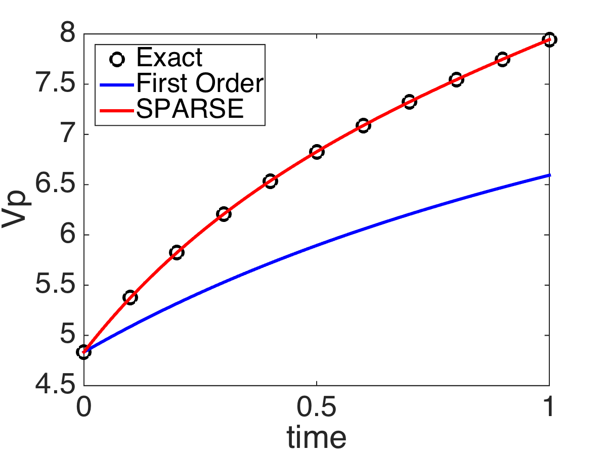
(a)

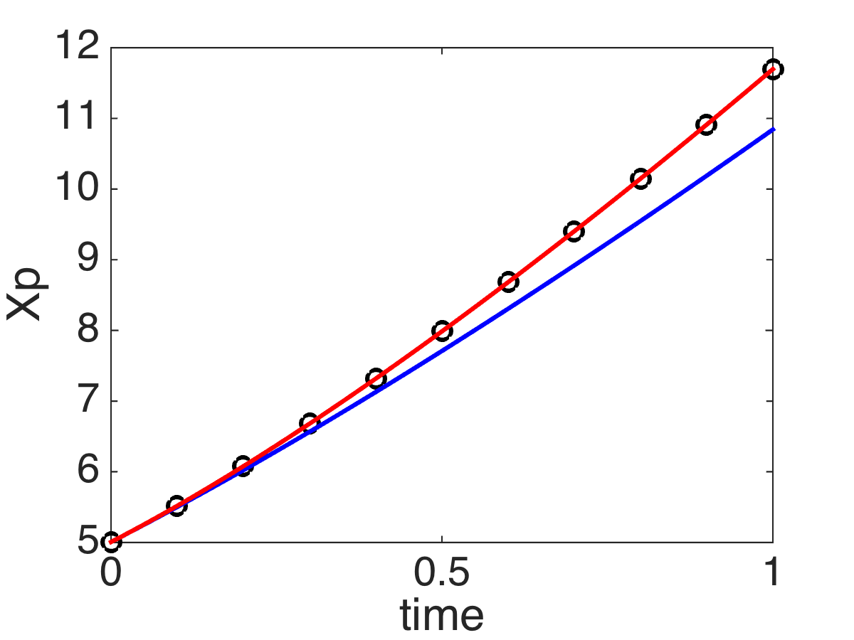
(b)

Figure 1: Particle (a) velocities and (b) locations using the mean of the exact particle locations as well as the First-Order and SPARSE models with a uniform background fluid velocity and a linear correction factor.

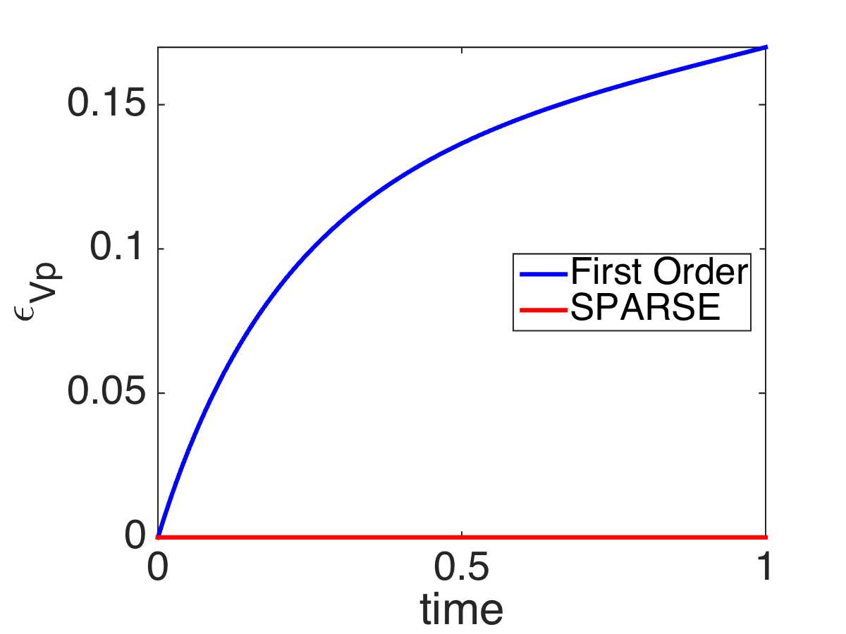
(a)

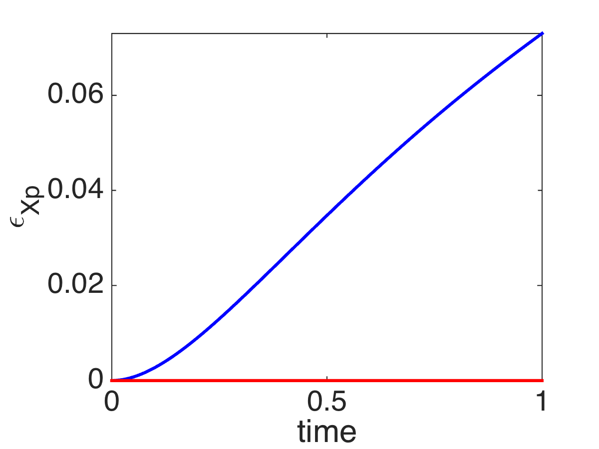
(b)

Figure 2: Modeling error of the mean particle (a) velocity and (b) location using the First-Order and SPARSE models with a uniform background fluid velocity and a linear correction factor.

For the initial conditions in (14), the interphase velocity difference can be negative and hence the correction factor in (15) can also have negative values. For a negative correction factor particles are nonphysically propelled.

Using the following correction factor of

$$f(a)=\frac{|a|}{10},$$ (17)

based on the absolute velocity, $|a|$, is more physical since $f(a)$ is always positive. Note that $f(a)$ in (17) is non-linear because of discontinuous derivatives at $a=0$.

The non-linearity leads to errors in the modeling of the average particle velocity with the SPARSE model (Figures 3(b) and 4). Because the SPARSE model accounts for the perturbations in the particle phase, it is still significantly more accurate than the First-Order model.

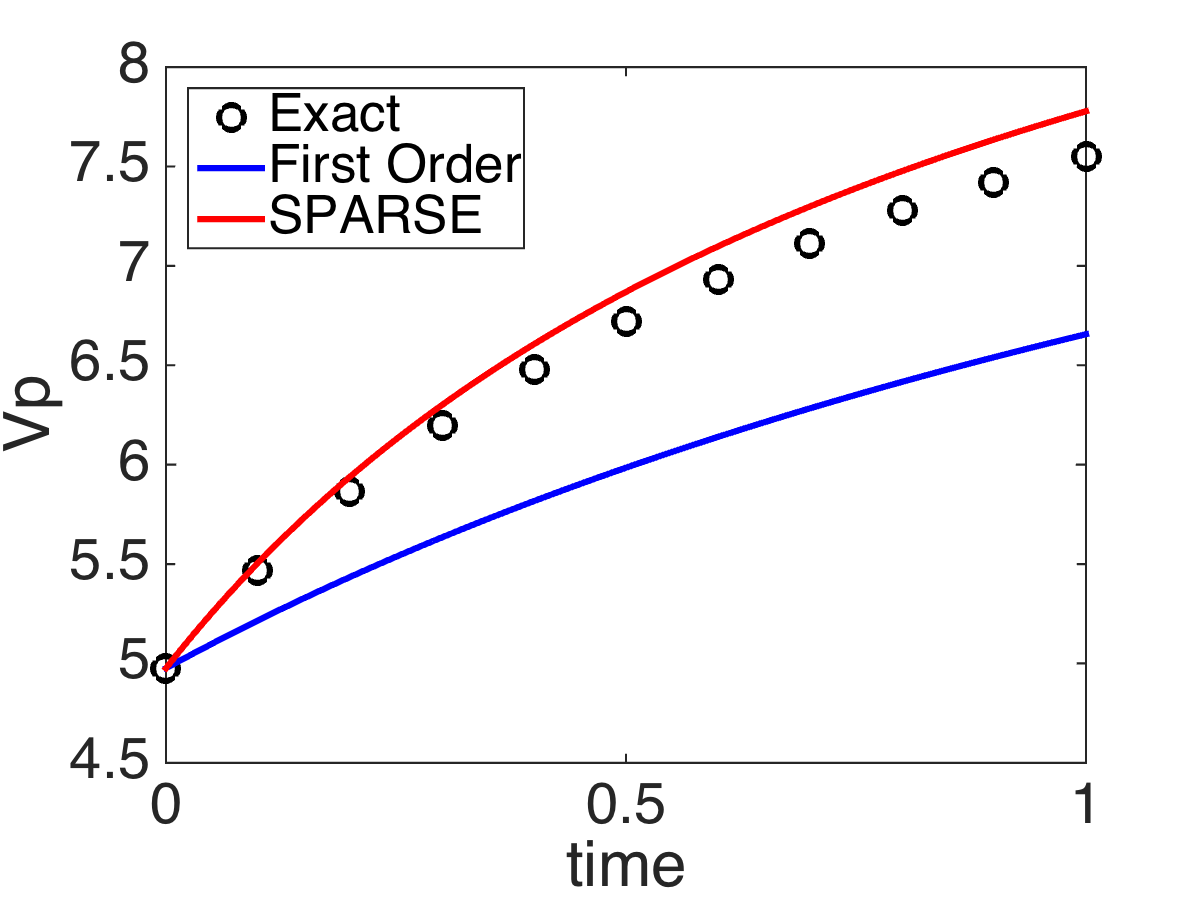
(a)

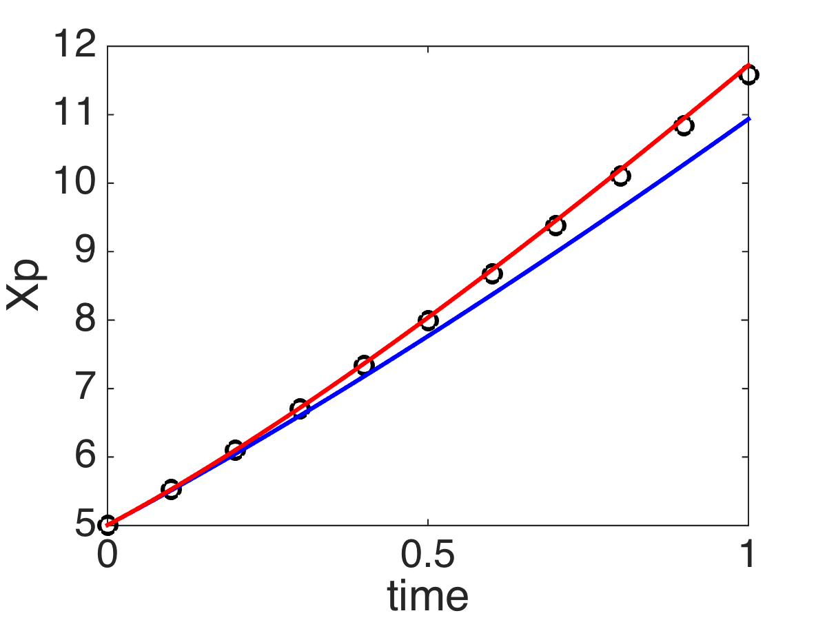
(b)

Figure 3: Particle (a) velocities and (b) locations using the mean of the exact particle locations as well as the First-Order and SPARSE models with a uniform background fluid velocity and an absolute value correction factor.

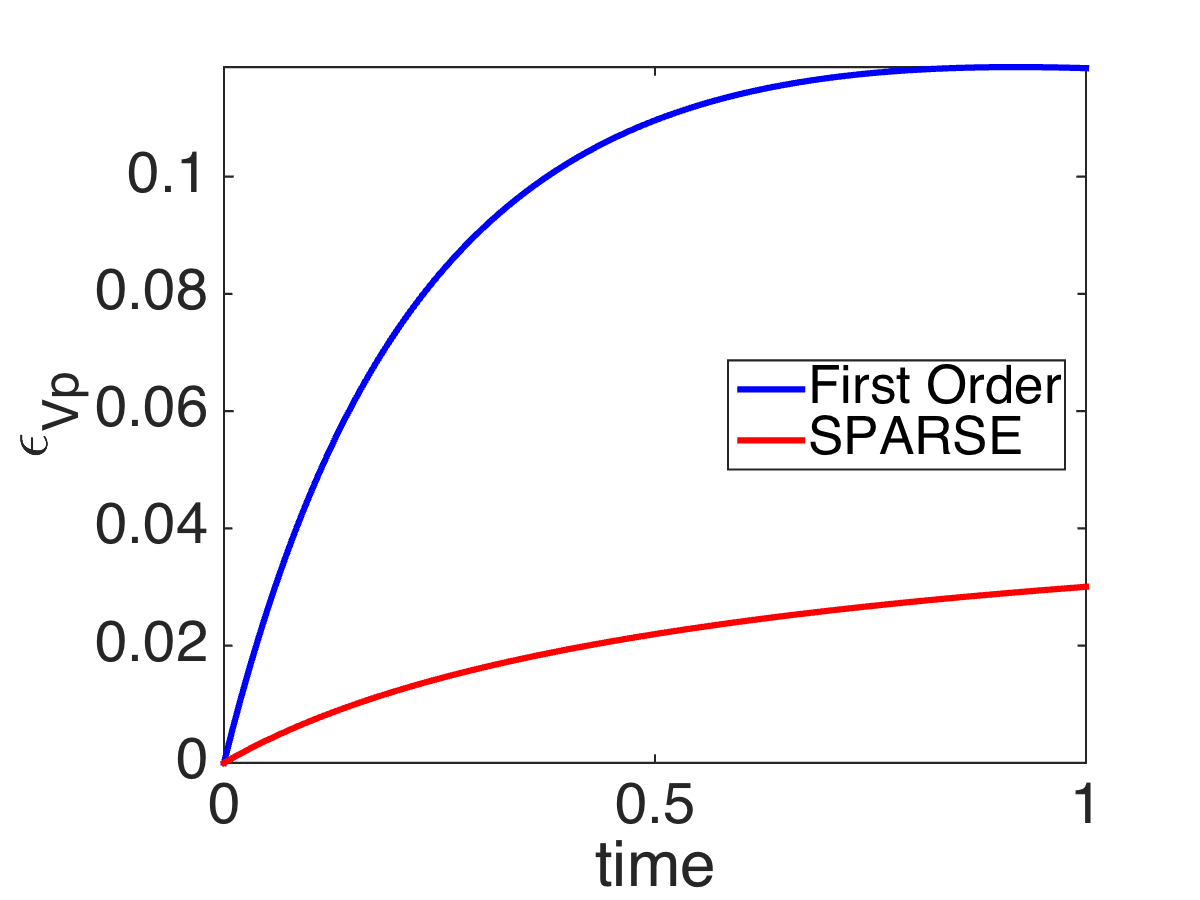
(a)

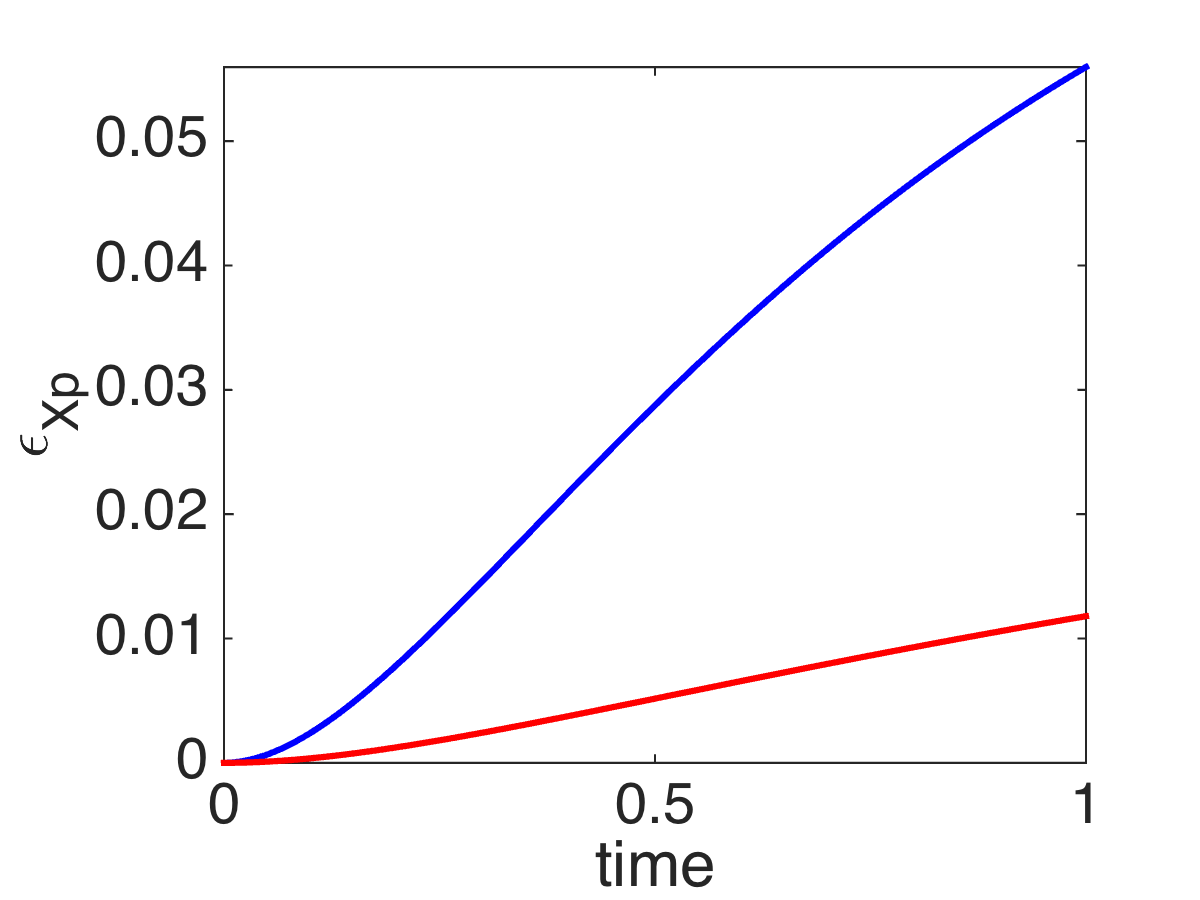
(b)

Figure 4: Modeling error of the mean particle (a) velocity and (b) location using the First-Order and SPARSE models with a uniform background fluid velocity and an absolute value correction factor.

3.2 Effect of Modeling the Average Cloud Velocity

To test the erroneous assumption that $\bar{u}({x}_{p})$ = $\bar{u}(\bar{x}_{p})$ in the First-Order model, a constant correction factor comparable to the Stokes’ drag [35] is used,

$$f(a)=\frac{24}{St}.$$ (18)

The combination of the constant correction factor, for which the Taylor expansions terms are zero, and a spatially varying carrier-phase velocity,

$$u(x)=\cos(\pi x)+x,$$ (19)

enables an investigation into the errors caused by the incorrect sampling of the carrier-phase velocity at a single point in the First-Order model.

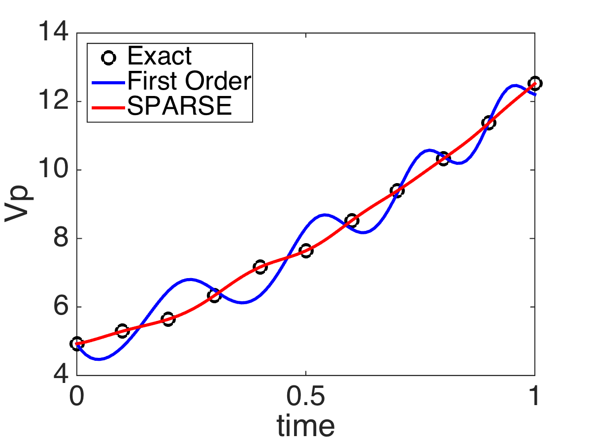
(a)

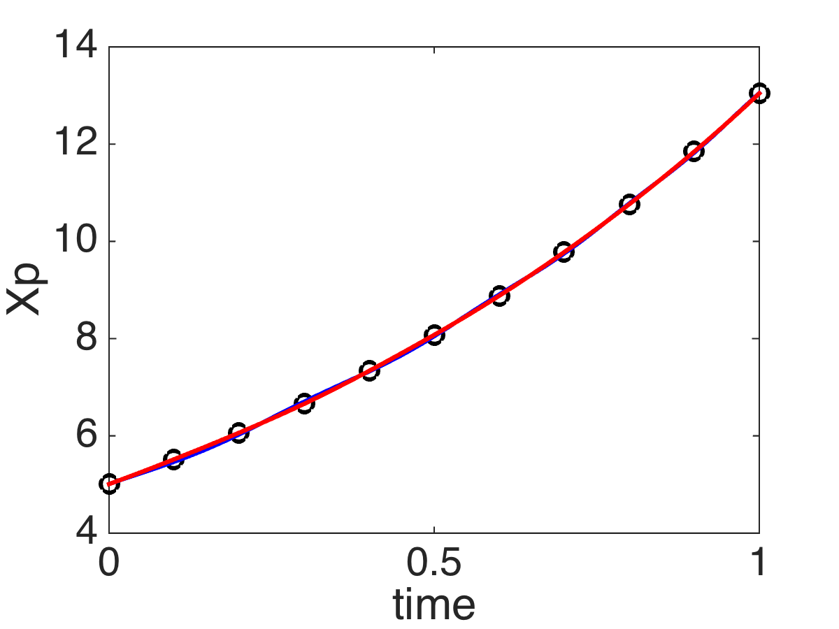
(b)

Figure 5: Particle (a) velocities and (b) locations using the mean of the exact particle locations as well as the First-Order and SPARSE models with a spatially varying background fluid velocity.

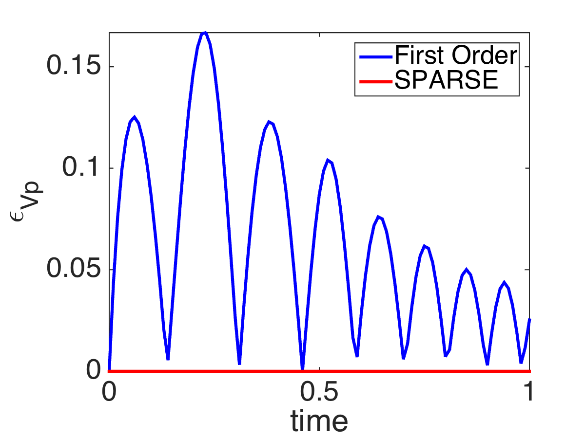
(a)

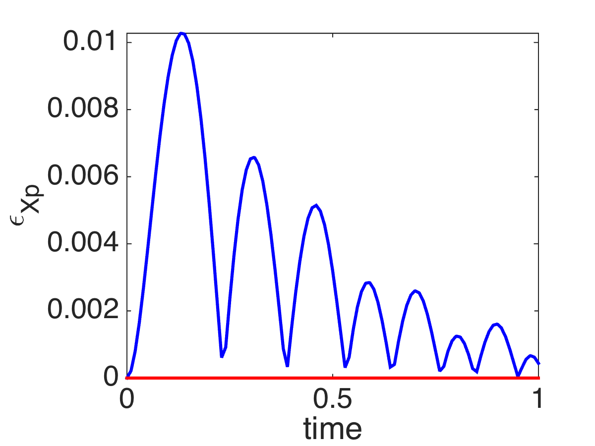
(b)

Figure 6: Modeling error of the mean particle (a) velocity and (b) location using the First-Order and SPARSE models with a spatially varying background fluid velocity.

Figures 5(a) and 6(a) shows that First-Order modeling of the fluid velocity can lead to errors as high as 17% whereas the averaged velocity and location of the cloud is a priori closed in an exact manner with the SPARSE model. Because the perturbations in the fluid velocity are periodic, the errors in the modeled particle velocity are oscillatory and only cause a maximum 1% error in the particle location in Figures 5(b) and 6(b).

4 Validation SPARSE: Decaying Isotropic Turbulence

To more rigorously test SPARSE a group of particles traced in a decaying isotropic turbulence according to the “exact” model is compared with the First-Order model and a priori closed SPARSE.

The isotropic turbulence simulation is performed in a cube with periodic boundary conditions on all sides. Following [36, 38] an initial correlated flow field is determined based on specified energy spectra. Computations are performed with a compressible Navier-Stokes solver based on a 4^th order central difference method for the fluxes (as described [4]). To verify the Navier-Stokes solver, we compare computations with this code with 128 cubed number of grid points with the case referred to as ”iga96” in [36] computed with a $N=96$ Fourier spectral method. The average initial fluctuating Mach number,

$$M_{0}=\frac{\sqrt{\overline{u_{i}^{\prime}u_{i}^{\prime}}}}{c(\overline{T_{0}})},$$ (20)

where $u_{i}^{\prime}$ is the fluctuating fluid velocity is set to $M_{0}=0.05$. The reference fluid Reynolds number is set to $Re_{f}=2357$. The decay of turbulent kinetic energy, TKE = $\frac{1}{2}\overline{{{u_{i}}^{\prime}}^{2}}$, in Figure 7 compares well with the results from Blaisdell et. al. [36]. The oscillatory trend in TKE is well-known and documented and is caused by pressure-dilation [39].

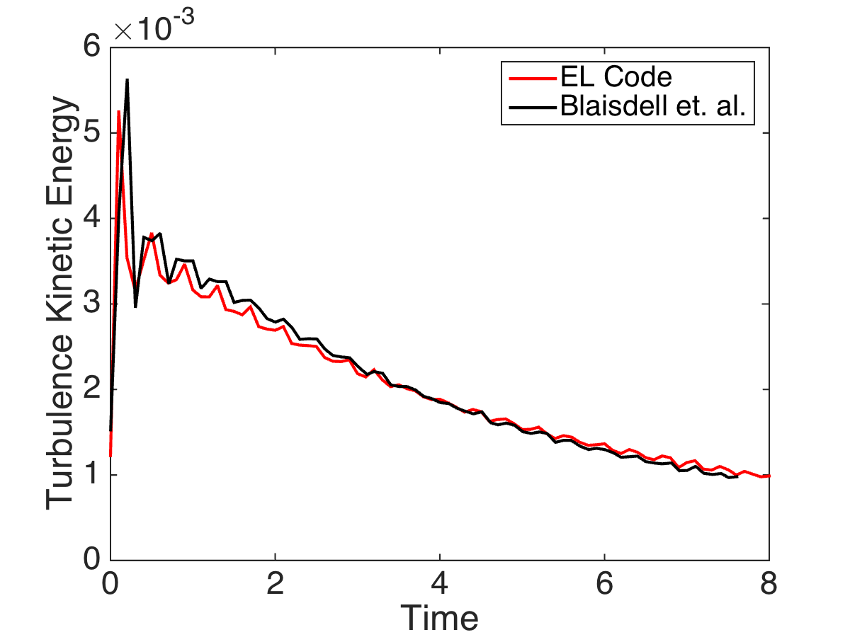
Figure 7: Comparison of the turbulent kinetic energy (TKE) versus time in isotropic turbulence using a high-order EL code from Jacobs et. al. [4] and a Fourier spectral method performed by Blaisdell et. al. [36].

To test the particle models an exact case that initializes $30^{3}=27,000$ particles uniformly over 3x3x3 grid cells, serves as a reference against which the First-Order model and SPARSE are tested. As compared to iga96 the initial velocity field is scaled by a factor five. This ensures that the carrier phase disperses the particle cloud more significantly than the iga96 velocity field and hence the effects of the cloud modeling are more visible. The initial particle velocity is set according to a uniform random number around zero with an absolute maximum of 2.5. We use the following drag correction function

$$C_{D}=\left(0.38+\frac{24}{Re_{p}}+\frac{4}{Re_{p}{\nicefrac{{1}}{{2}}}}\right)\left(1+e^{-\frac{0.43}{M_{p}^{4.67}}}\right),$$ (21)

that corrects the Stokes drag for high relative particle Reynolds number, $Re_{p}=|v_{f}-v_{p}|d_{p}/\nu$, and Mach number, $M_{p}=|v_{f}-v_{p}|/\sqrt{T_{f}}$, according to Boiko et. al. [32, 4, 6, 7, 40]. The particles’ response time is set to $\tau_{p}=0.01$. Matlab was used to compute the partial derivatives of the drag coefficient equation, which are needed for the SPARSE model in (12).

The time lapse in Figure 8 shows that the cloud modeled with SPARSE (red sphere) closely follows the average location of the exact cloud (green sphere), while the First-Order model (red sphere) deviates significantly from the exact cloud. The temporal dispersion of the exact cloud is visualized by the large diameter of the exact model (green) sphere as compared to initial diameter of the (red and blue) cloud approaches. Dispersion, as measured by for example the rate of change of the cloud radius, is not modeled in the SPARSE and First-Order model and it is the subject of ongoing investigation.

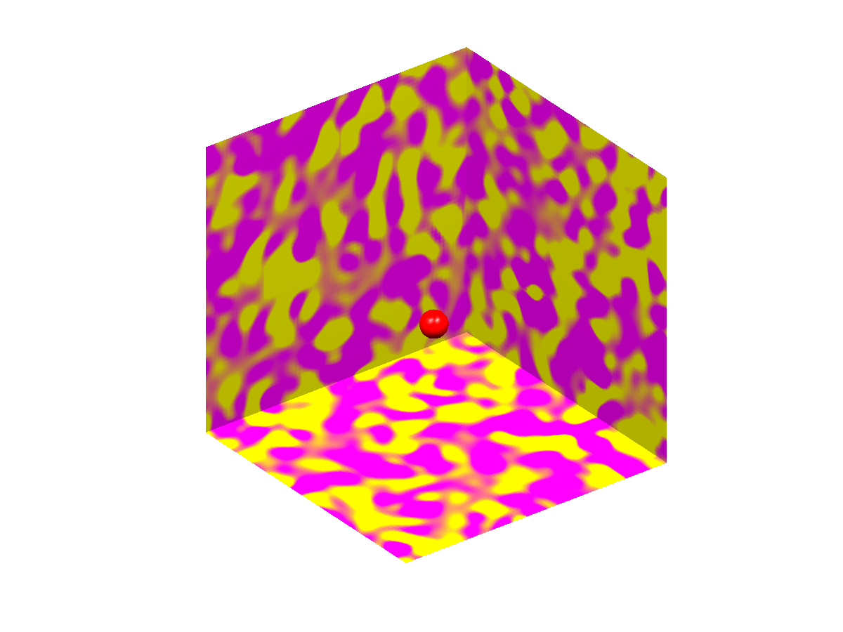
(a) t = 0

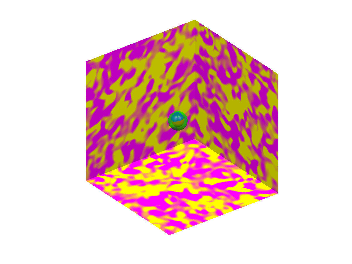
(b) t = 2

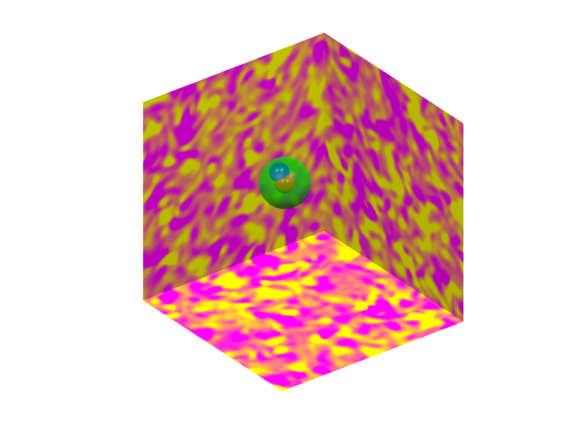
(c) t = 4

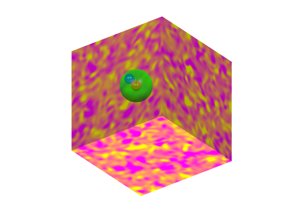
(d) t = 6

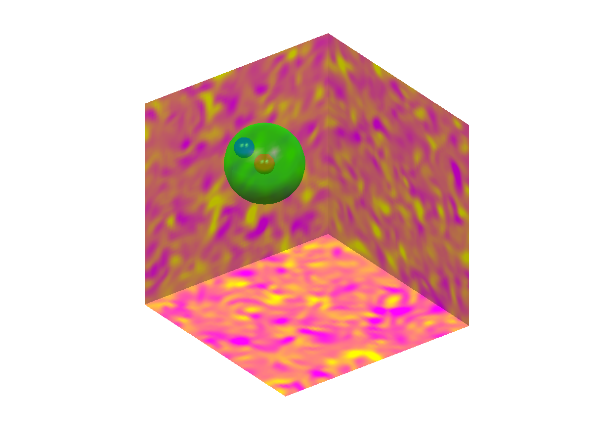
(e) t = 8

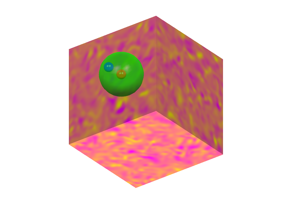
(f) t = 10

Figure 8: Helicity projected onto the cubical computational domain faces and particle cloud locations for the 3D isotropic decaying turbulence case at times t = (a) 0.0, (b) 1.6, (c) 3.2, (d) 4.8, (e) 6.4 and (f) 8.0. The First-Order modeled particle is visualized by a blue sphere, the SPARSE modeled by a red (sphere) and the exact model by a green sphere. The root mean square dispersion of the the exact location is visualized by the diameter of the green sphere. The diameter of the red and blue sphere visualize the initial rms dispersion.

A comparison of the average particle cloud distance from the origin

$$|{\bf x_{p}}|=\sqrt{x_{p}^{2}+y_{p}^{2}+z_{p}^{2}},$$

and averaged velocity,

$$|{\bf v_{p}}|=\sqrt{u_{p}^{2}+v_{p}^{2}+w_{p}^{2}},$$ (22)

in Figure 9 confirms the improved modeling by SPARSE as compared to the First-Order model. While both the exact cloud and the computational clouds are initially entrained in the same turbulent eddy, the average velocity over the cloud used in SPARSE is near zero, while the local velocity used in the First-Order model is large. The latter cloud is hence displaced more. With increasing time, the exact cloud disperses and the fluid velocity is sampled over a larger area. Because the turbulence is isotropic and decaying the averaged fluid velocity goes to zero over a larger area and increasing time, respectively. The local velocity decays in time also, but deviates from the near zero, averaged velocity leading to the deviation of the First-Order model in time.

Errors in the magnitude of the distance from the origin and velocity plotted in Figure 10 shows that SPARSE modeling errors are non-zero, because the drag correction in (21)is non-linear and hence the Taylor truncation error in (10) used for SPARSE is non-zero. The error however is small, within 0.5% of the exact model.

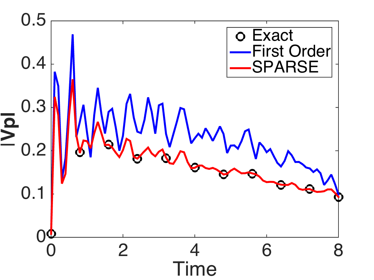
(a)

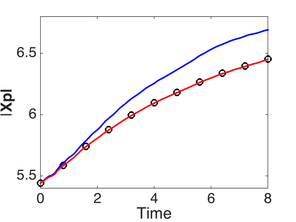
(b)

Figure 9: The magnitude of the average (a) velocity and (b) particle distance from the origin is shown when computed using the First-Order model, SPARSE model and average over the physical particles.

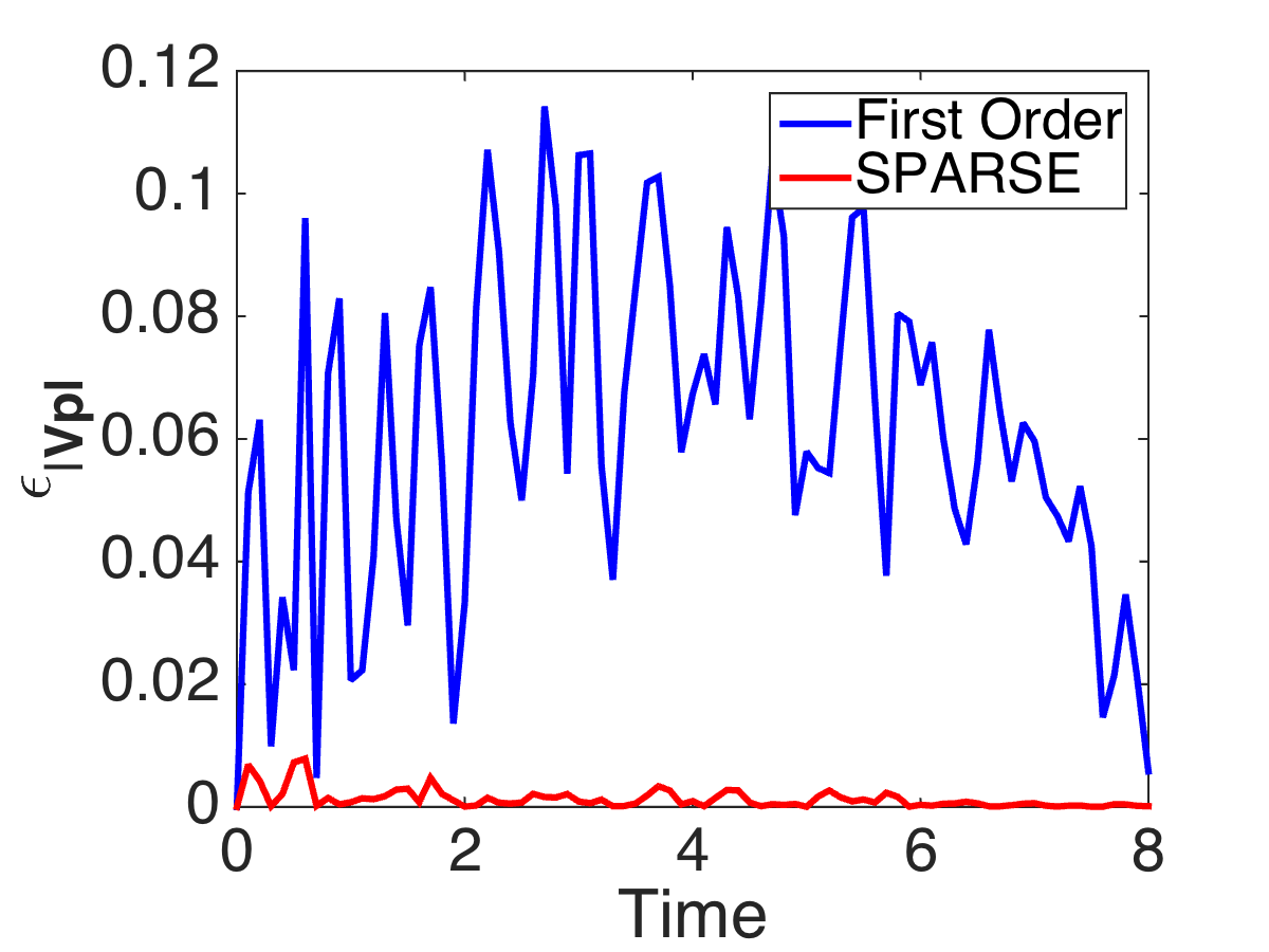
(a)

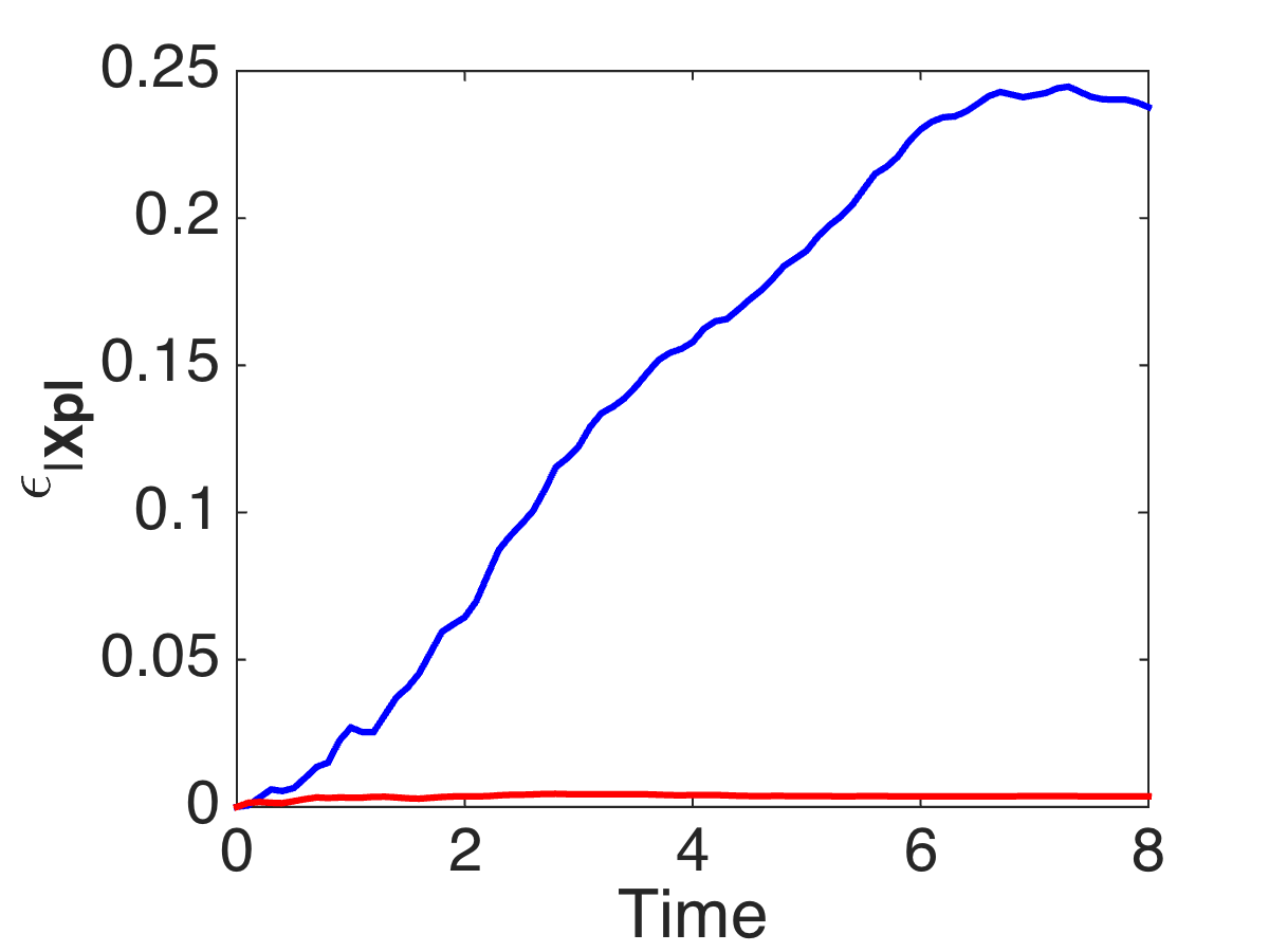
(b)

ma

Figure 10: The error in computing the magnitude of the average (a) velocity and (b) particle distance from the origin is shown when computed using the First-Order model, SPARSE model and average over the physical particles.

The impact of two modeling components of the SPARSE model, including the averaging of the fluid velocity of the cloud and the stress modeling are compared in Figure 12. Plotted are the two terms on the right-hand side of (12). The first term that is affected by the cloud velocity averaging is significantly larger than the second term that is proportional to the sub-cloud stresses. The second term is on the order of $10^{-5}$. In general, the effect of the sub-cloud stresses is not necesarilly smaller than the effect of velocity averaging as was seen in the 1D tests.

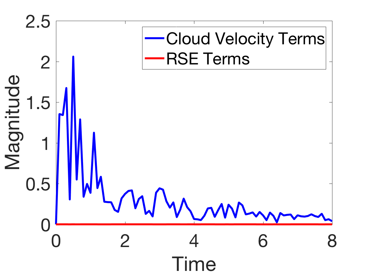
Figure 11:

Figure 12: Comparison of the two terms on the right hand side of (12, $f(\bar{\bf a})\bar{\bf a}$ and $\frac{df(\bar{\bf a})}{d{\bf a}}\overline{{\bf a}^{\prime}{\bf a}^{\prime}}$. The first term (blue line) is dependend on the SPARSE fluid velocity modeling and the second term (red line) is proportional to the interphase stresses.

5 Conclusions and Future Work

SPARSE provides a model that traces a group of point particles through a single computational point parcel. The model improves upon Cloud-In-Cell methods by, firstly, accounting for fluid and particle stress (i.e. the Reynolds stress equivalent) terms and, secondly, averaging of the fluid velocity at the Lagrangian computational particle. One-dimensional and three-dimensional a priori tests show that both improvements yield an excellent comparison of the averaged trace of a cloud of particles and the computational parcel.

This paper is only a first step in the development of a closed SPARSE model. Current investigation focuses on closure based on a multi-scale approach as reported in [31].

References

- [1] C. T. Crowe, M. P. Sharma, D. E. Stock, The Particle-Source in Cell (PSI-Cell) model for gas-droplet flows, J. Fluids Eng. 6 (1977) 325–332.
- [2] C. Crowe, M. Sommerfeld, Y. Tsuji, Multiphase flows with droplets and particles, CRC Press, 1998.
- [3] C. K. Birdsall, D. Fuss, Clouds-in-clouds, clouds-in-cells physics for many-body plasma simulation, Journal of Computational Physics 3 (4) (1969) 494–511.
- [4] G. B. Jacobs, W.-S. Don, A high-order WENO-Z finite difference based particle-source-in-cell method for computation of particle-laden flows with shocks, Journal of Computational Physics 228 (5) (2009) 1365 – 1379.
- [5] G. B. Jacobs, W. S. Don, T. Dittmann, High-order resolution Eulerian-Lagrangian simulations of particle dispersion in the accelerated flow behind a moving shock, Theor. Comput. Fluid Dyn. 26 (1-4) (2012) 37–50.
- [6] S. Davis, T. Dittman, G. B. Jacobs, W. S. Don, High-fidelity Eulerian-Lagrangian methods for simulation of three-dimensional, unsteady, high-speed, two-phase flows in high-speed combustors, in: 47th AIAA/ASME/SAE/ASEE Joint Propulsion Conference, 2011.
- [7] S. Davis, T. Dittmann, G. Jacobs, W. Don, Dispersion of a cloud of particles by a moving shock: Effects of the shape, angle of rotation, and aspect ratio, Journal of Applied Mechanics and Technical Physics 54 (6) (2013) 900–912.
- [8] J. Smagorinsky, General circulation experiments with the primitive equations: I. the basic experiment*, Monthly weather review 91 (3) (1963) 99–164.
- [9] M. Germano, U. Piomelli, P. Moin, W. H. Cabot, A dynamic subgrid‐scale eddy viscosity model, Physics of Fluids A 3 (7) (1991) 1760–1765.
- [10] B. Launder, D. Spalding, The numerical computation of turbulent flows, Computer Methods in Applied Mechanics and Engineering 3 (2) (1974) 269 – 289. doi:http://dx.doi.org/10.1016/0045-7825(74)90029-2.
- [11] F. R. Menter, Two-equation eddy-viscosity turbulence models for engineering applications, AIAA Journal 32 (8) (1994) 1598–1605. doi:10.2514/3.12149.
- [12] G. Erlebacher, M. Hussaini, H. Kreiss, S. Sarkar, The analysis and simulation of compressible turbulence, Theoretical and Computational Fluid Dynamics 2 (2) (1990) 73–95.
- [13] C. G. Speziale, S. Sarkar, T. B. Gatski, Modelling the pressure–strain correlation of turbulence: an invariant dynamical systems approach, Journal of Fluid Mechanics 227 (1991) 245–272.
- [14] V. Armenio, S. Sarkar, An investigation of stably stratified turbulent channel flow using Large-Eddy Simulation, Journal of Fluid Mechanics 459 (2002) 1–42. doi:10.1017/S0022112002007851.
- [15] B. Shotorban, Modeling of subgrid-scale effects on particles in Large-Eddy simulation of turbulent two-phase flows, Ph.D. thesis, University of Illinois at Chicago (2005).
- [16] J. Kuerten, A. Verman, Can turbophoresis be predicted by Large-Eddy Simulation?, Physics of Fluids, 17 (1) (2005) 011701–011701.
- [17] B. Shotorban, F. Mashayek, Modeling subgrid-scale effects on particles by approximate deconvolution, Physics of Fluids (1994-present) 17 (8) (2005a) 081701.
- [18] J. Kuerten, Subgrid modeling in particle-laden channel flow, Physics of Fluids, 18 (2) (2006) 025108.
- [19] B. Shotorban, K. Zhang, F. Mashayek, Improvement of particle concentration prediction in Large-Eddy Simulation by defiltering, International journal of heat and mass transfer 50 (19) (2007) 3728–3739.
- [20] S. Stolz, N. Adams, L. Kleiser, An approximate deconvolution model for Large-Eddy Simulation with application to incompressible wall-bounded flows, Physics of Fluids, 13 (4) (2001) 997–1015.
- [21] B. Shotorban, A. Afshari, F. Jaberi, F. Mashayek, A particle tracking algorithm for les of two-phase flow, AIAA Paper 332.
- [22] B. Shotorban, S. Balachandar, Particle concentration in homogeneous shear turbulence simulated via Lagrangian and equilibrium eulerian approaches, Physics of Fluids, 18 (6) (2006) 065105.
- [23] J. Pozorski, J.-P. Minier, On the Lagrangian turbulent dispersion models based on the langevin equation, International Journal of Multiphase Flow 24 (6) (1998) 913–945.
- [24] J. Pozorski, J.-P. Minier, Probability density function modeling of dispersed two-phase turbulent flows, Physical Review E 59 (1) (1999) 855.
- [25] J.-P. Minier, E. Peirano, The PDF approach to turbulent polydispersed two-phase flows, Physics reports 352 (1) (2001) 1–214.
- [26] L. Y. Gicquel, P. Givi, F. Jaberi, S. Pope, Velocity filtered density function for Large-Eddy Simulation of turbulent flows, Physics of Fluids, 14 (3) (2002) 1196–1213.
- [27] A. Berrouk, D. Laurence, J. Riley, D. Stock, Stochastic modelling of inertial particle dispersion by subgrid motion for LES of high Reynolds number pipe flow, Journal of Turbulence (8) (2007).
- [28] C. P. Chen, P. E. Wood, A turbulence closure model for dilute gas-particle flows, The Canadian Journal of Chemical Engineering 63 (3) (1985) 349–360. doi:10.1002/cjce.5450630301.
- [29] A. Mostafa, H. Mongia, On the interaction of particles and turbulent fluid flow, International Journal of Heat and Mass Transfer 31 (10) (1988) 2063 – 2075. doi:http://dx.doi.org/10.1016/0017-9310(88)90117-2.
- [30] J. Tu, C. Fletcher, An improved model for particulate turbulence modulation in confined two-phase flows, International Communications in Heat and Mass Transfer 21 (6) (1994) 775 – 783. doi:http://dx.doi.org/10.1016/0735-1933(94)90031-0.
- [31] O. Sen, S. L. Davis, G. .B Jacobs, H. S. Udaykumar, Evaluation of convergence behavior of metamodeling techniques for bridging scales in multi-scale multimaterial simulation, Journal of Computational Physics 294 (2015), 585–604.
- [32] V. Boiko, V. P. Kiselev, S. P. Kiselev, A. Papyrin, S. Poplavsky, V. Fomin, Shock wave interaction with a cloud of particles, Shock Waves 7 (1997) 275–285.
- [33] X. Tong, M. Remotigue, E. Luke, J. Kang, ”Multiphase simulations of blast-soil interactions, in: Proceedings of the ASME 2013 Fluids Engineering Division”, Summer Meeting, ASME, (2013), No. FEDSM2013-16549.
- [34] L. Schiller, A. Naumann, A drag coefficient correlation, VDI Zeitschrift 77 (1933) 318–320.
- [35] G. G. Stokes, On the effect of the internal friction of fluids on the motion of pendulums., Transactions of the Cambridge Philosophical Society 9.
- [36] G. A. Blaisdell, Numerical simulation of compressible homogeneous turbulence, Ph.D. thesis, Stanford Univ., CA. (1991).
- [37] G. A. Blaisdell, N. N. Mansour, W. C. Reynolds, Compressibility effects on the growth and structure of homogeneous turbulent shear flow, Journal of Fluid Mechanics 256 (1993) 443–485. doi:10.1017/S0022112093002848.
- [38] G. B. Jacobs, D. A. Kopriva, F. Mashayek, “Validation Study of a Multidomain Spectral Code for Simulation of TUrbulent Flows“, , AIAA Journal 43 (6) (2005) 1256–1264.
- [39] S. Kida, S. Orszag, Energy and spectral dynamics in decaying compressible turbulence, Journal of Scientific Computing 7 (1) (1992) 1–34. doi:10.1007/BF01060209.
- [40] S. Davis, G. Jacobs, W. Don, Carbuncles in high resolution Eulerian-Lagrangian simulation of shock-particle-laden flow, 21st AIAA CFD Conference.