Simultaneous Learning of Trees and Representations for Extreme Classification and Density Estimation

Abstract

We consider multi-class classification where the predictor has a hierarchical structure that allows for a very large number of labels both at train and test time. The predictive power of such models can heavily depend on the structure of the tree, and although past work showed how to learn the tree structure, it expected that the feature vectors remained static. We provide a novel algorithm to simultaneously perform representation learning for the input data and learning of the hierarchical predictor. Our approach optimizes an objective function which favors balanced and easily-separable multi-way node partitions. We theoretically analyze this objective, showing that it gives rise to a boosting style property and a bound on classification error. We next show how to extend the algorithm to conditional density estimation. We empirically validate both variants of the algorithm on text classification and language modeling, respectively, and show that they compare favorably to common baselines in terms of accuracy and running time.

1 Introduction

Several machine learning settings are concerned with performing predictions in a very large discrete label space. From extreme multi-class classification to language modeling, one commonly used approach to this problem reduces it to a series of choices in a tree-structured model, where the leaves typically correspond to labels. While this allows for faster prediction, and is in many cases necessary to make the models tractable, the performance of the system can depend significantly on the structure of the tree used, e.g. (Mnih & Hinton, 2009).

Instead of relying on possibly costly heuristics (Mnih & Hinton, 2009), extrinsic hierarchies (Morin & Bengio, 2005) which can badly generalize across different data sets, or purely random trees, we provide an efficient data-dependent algorithm for tree construction and training. Inspired by the LOM tree algorithm (Choromanska & Langford, 2015) for binary trees, we present an objective function which favors high-quality node splits, i.e. balanced and easily separable. In contrast to previous work, our objective applies to trees of arbitrary width and leads to guarantees on model accuracy. Furthermore, we show how to successfully optimize it in the setting when the data representation needs to be learned simultaneously with the classification tree.

Finally, the multi-class classification problem is closely related to that of conditional density estimation (Ram & Gray, 2011; Bishop, 2006) since both need to consider all labels (at least implicitly) during learning and at prediction time. Both problems present similar difficulties when dealing with very large label spaces, and the techniques that we present in this work can be applied indiscriminately to either. Indeed, we show how to adapt our algorithm to efficiently solve the conditional density estimation problem of learning a language model which uses a tree structured objective.

This paper is organized as follows: Section 2 discusses related work, Section 3 outlines the necessary background and defines the flat and tree-structured objectives for multi-class classification and density estimation, Section 4 presents the objective and the optimization algorithm, Section 5 contains theoretical results, Section 6 adapts the algorithm to the problem of language modeling, Section 7 reports empirical results on the Flickr tag prediction dataset and Gutenberg text corpus, and finally Section 8 concludes the paper. Supplementary material contains additional material and proofs of theoretical statements of the paper. We also release the C++ implementation of our algorithm.

2 Related Work

The multi-class classification problem has been addressed in the literature in a variety of ways. Some examples include i) clustering methods (Bengio et al., 2010; Madzarov et al., 2009; Weston et al., 2013) ((Bengio et al., 2010) was later improved in (Deng et al., 2011)), ii) sparse output coding (Zhao & Xing, 2013), iii) variants of error correcting output codes (Hsu et al., 2009), iv) variants of iterative least-squares (Agarwal et al., 2014), v) a method based on guess-averse loss functions (Beijbom et al., 2014), and vi) classification trees (Beygelzimer et al., 2009b; Choromanska & Langford, 2015; Daume et al., 2016) (that includes the Conditional Probability Trees (Beygelzimer et al., 2009a) when extended to the classification setting).

The recently proposed LOM tree algorithm (Choromanska & Langford, 2015) differs significantly from other similar hierarchical approaches, like for example Filter Trees (Beygelzimer et al., 2009b) or random trees (Breiman, 2001), in that it addresses the problem of learning good-quality binary node partitions. The method results in low-entropy trees and instead of using an inefficient enumerate-and-test approach, see e.g: (Breiman et al., 1984), to find a good partition or expensive brute-force optimization (Agarwal et al., 2013), it searches the space of all possible partitions with SGD (Bottou, 1998). Another work (Daume et al., 2016) uses a binary tree to map an example to a small subset of candidate labels and makes a final prediction via a more tractable one-against-all classifier, where this subset is identified with the proposed Recall Tree. A notable approach based on decision trees also include FastXML (Prabhu & Varma, 2014) (and its slower and less accurate at prediction predecessor (Agarwal et al., 2013)). It is based on optimizing the rank-sensitive loss function and shows an advantage over some other ranking and NLP-based techniques in the context of multi-label classification. Other related approaches include the SLEEC classifier (Bhatia et al., 2015) for extreme multi-label classification that learns embeddings which preserve pairwise distances between only the nearest label vectors and ranking approaches based on negative sampling (Weston et al., 2011). Another tree approach (Kontschieder et al., 2015) shows no computational speed up but leads to significant improvements in prediction accuracy.

Conditional density estimation can also be challenging in settings where the label space is large. The underlying problem here consists in learning a probability distribution over a set of random variables given some context. For example, in the language modeling setting one can learn the probability of a word given the previous text, either by making a Markov assumption and approximating the left context by the last few words seen (n-grams e.g. (Jelinek & Mercer, 1980; Katz, 1987), feed-forward neural language models  (Mnih & Teh, 2012; Mikolov et al., 2011; Schwenk & Gauvain, 2002)), or by attempting to learn a low-dimensional representation of the full history (RNNs (Mikolov et al., 2010; Mirowski & Vlachos, 2015; Tai et al., 2015; Kumar et al., 2015)). Both the recurrent and feed-forward Neural Probabilistic Language Models (NPLM) (Bengio et al., 2003) simultaneously learn a distributed representation for words and the probability function for word sequences, expressed in terms of these representations. The major drawback of these models is that they can be slow to train, as they grow linearly with the vocabulary size (anywhere between 10,000 and 1M words), which can make them difficult to apply (Mnih & Teh, 2012). A number of methods have been proposed to overcome this difficulty. Works such as LBL (Mnih & Hinton, 2007) or Word2Vec (Mikolov et al., 2013) reduce the model to its barest bones, with only one hidden layer and no non-linearities. Another proposed approach has been to only compute the NPLM probabilities for a reduced vocabulary size, and use hybrid neural-$n$-gram model (Schwenk & Gauvain, 2005) at prediction time. Other avenues to reduce the cost of computing gradients for large vocabularies include using different sampling techniques to approximate it (Bengio & Sénécal, 2003; Bengio & Senecal, 2008; Mnih & Teh, 2012), replacing the likelihood objective by a contrastive one (Gutmann & Hyvärinen, 2012) or spherical loss (de Brébisson & Vincent, 2016), relying on self-normalizing models (Andreas & Klein, 2015), taking advantage of data sparsity  (Vincent et al., 2015), or using clustering-based methods (Grave et al., 2016). It should be noted however that most of these techniques (to the exception of (Grave et al., 2016)) do not provide any speed up at test time.

Similarly to the classification case, there have also been a significant number of works that use tree structured models to accelerate computation of the likelihood and gradients (Morin & Bengio, 2005; Mnih & Hinton, 2009; Djuric et al., 2015; Mikolov et al., 2013). These use various heuristics to build a hierarchy, from using ontologies (Morin & Bengio, 2005) to Huffman coding (Mikolov et al., 2013). One algorithm which endeavors to learn a binary tree structure along with the representation is presented in  (Mnih & Hinton, 2009). They iteratively learn word representations given a fixed tree structure, and use a criterion that trades off between making a balanced tree and clustering the words based on their current embedding. The application we present in the second part of our paper is most closely related to the latter work, and uses a similar embedding of the context. However, where their setting is limited to binary trees, we work with arbitrary width, and provide a tree building objective which is both less computationally costly and comes with theoretical guarantees.

3 Background

In this section, we define the classification and log-likelihood objectives we wish to maximize. Let $\mathcal{X}$ be an input space, and $\mathcal{V}$ a label space. Let $\mathcal{P}$ be a joint distribution over samples in $(\mathcal{X},\mathcal{V})$, and let $f_{\Theta}:\mathcal{X}\rightarrow\mathbb{R}^{d_{r}}$ be a function mapping every input $x\in\mathcal{X}$ to a representation $\mathbf{r}\in\mathbb{R}^{d_{r}}$, and parametrized by $\Theta$ (e.g. as a neural network).

We consider two objectives. Let $g$ be a function that takes an input representation $\mathbf{r}\in\mathbb{R}^{d_{r}}$, and predicts for it a label ${g(\mathbf{r})\in\mathcal{V}}$. The classification objective is defined as the expected proportion of correctly classified examples:

$$\mathcal{O^{\text{class}}}(\Theta,g)={\mathbb{E}}_{(x,y)\sim\mathcal{P}}\Big{[}{\mathbbm{1}}[g\circ f_{\Theta}(x)=y]\Big{]}\vspace{-0.05in}$$ (1)

Now, let $p_{\theta}(\cdot|\mathbf{r})$ define a conditional probability distribution (parametrized by $\theta$) over $\mathcal{V}$ for any $\mathbf{r}\in\mathbb{R}^{d_{r}}$. The density estimation task consists in maximizing the expected log-likelihood of samples from $(\mathcal{X},\mathcal{V})$:

$$\mathcal{O^{\text{ll}}}(\Theta,\theta)={\mathbb{E}}_{(x,y)\sim\mathcal{P}}\Big{[}\log p_{\theta}(y|f_{\Theta}(x))\Big{]}$$ (2)

Tree-Structured Classification and Density Estimation

Let us now show how to express the objectives in Equations 1 and 2 when using tree-structured prediction functions (with fixed structure) as illustrated in Figure 1.

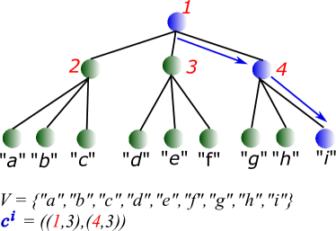
Figure 1: Hierarchical predictor: in order to predict label “$i$”, the system needs to choose the third child of node $1$, then the third child of node $4$.

Consider a tree $\mathcal{T}$ of depth $D$ and arity $M$ with $K=|\mathcal{V}|$ leaf nodes and $N$ internal nodes. Each leaf $l$ corresponds to a label, and can be identified with the path $\mathbf{c}^{l}$ from the root to the leaf. In the rest of the paper, we will use the following notations:

$$\mathbf{c}^{l}=((c^{l}_{1,1},c^{l}_{1,2}),\ldots,(c^{l}_{d,1},c^{l}_{d,2}),\ldots,(c^{l}_{D,1},c^{l}_{D,2})),\vspace{-0.05in}$$ (3)

where $c^{l}_{d,1}\in[1,N]$ correspond to the node index at depth $d$, and $c^{l}_{d,2}\in[1,M]$ indicates which child of $c^{l}_{d,1}$ is next in the path. In that case, our classification and density estimation problems are reduced to choosing the right child of a node or defining a probability distribution over children given $x\in\mathcal{X}$ respectively.

We then need to replace $g$ and $p_{\theta}$ with node decision functions $(g_{n})_{n=1}^{N}$ and conditional probability distributions $(p_{\theta_{n}})_{n=1}^{N}$ respectively. Given such a tree and representation function, our objective functions then become:

$$\mathcal{O^{\text{class}}}(\Theta,g)={\mathbb{E}}_{(x,y)\sim\mathcal{P}}\Big{[}\prod_{d=1}^{D}{\mathbbm{1}}[g_{c^{l}_{d,1}}\circ f_{\Theta}(x)=c^{l}_{d,2}]\Big{]}$$ (4)

$$\mathcal{O^{\text{ll}}}(\Theta,\theta)={\mathbb{E}}_{(x,y)\sim\mathcal{P}}\Big{[}\sum_{d=1}^{D}\log p_{\theta_{c^{l}_{d,1}}}(c^{l}_{d,2}|f_{\Theta}(x))\Big{]}$$ (5)

The tree objectives defined in Equations 4 and 5 can be optimized in the space of parameters of the representation and node functions using standard gradient ascent methods. However, they also implicitly depend on the tree structure $\mathcal{T}$. In the rest of the paper, we provide a surrogate objective function which determines the structure of the tree and, as we show theoretically (Section 5), maximizes the criterion in Equation 4 and, as we show empirically (Sections 6 and 7), maximizes the criterion in Equation 5.

4 Learning Tree-Structured Objectives

In this section, we introduce a per-node objective $J_{n}$ which leads to good quality trees when maximized, and provide an algorithm to optimize it.

4.1 Objective function

We define the node objective $J_{n}$ for node $n$ as:

$$J_{n}=\frac{2}{M}\sum_{i=1}^{K}q^{(n)}_{i}\sum_{j=1}^{M}|p^{(n)}_{j}-p^{(n)}_{j|i}|,\vspace{-0.14in}$$ (6)

where $q^{(n)}_{i}$ denotes the proportion of nodes reaching node $n$ that are of class $i$, $p^{(n)}_{j|i}$ is the probability that an example of class $i$ reaching $n$ will be sent to its $j^{\text{th}}$ child, and $p^{(n)}_{j}$ is the probability that an example of any class reaching $n$ will be sent to its $j^{\text{th}}$ child. Note that we have:

$$\forall j\in[1,M],\;\;p^{(n)}_{j}=\sum_{i=1}^{K}q^{(n)}_{i}p^{(n)}_{j|i}.\vspace{-0.1in}$$ (7)

The objective in Equation 6 reduces to the LOM tree objective in the case of $M=2$.

At a high level, maximizing the objective encourages the conditional distribution for each class to be as different as possible from the global one; so the node decision function needs to be able to discriminate between examples of the different classes. The objective thus favors balanced and pure node splits. To wit, we call a split at node $n$ perfectly balanced when the global distribution $p_{\cdot}^{(n)}$ is uniform, and perfectly pure when each $p^{(n)}_{\cdot|i}$ takes value either $0$ or $1$, as all data points from the same class reaching node $n$ are sent to the same child.

In Section 5 we discuss the theoretical properties of this objective in details. We show that maximizing it leads to perfectly balanced and perfectly pure splits. We also derive the boosting theorem that shows the number of internal nodes that the tree needs to have to reduce the classification error below any arbitrary threshold, under the assumption that the objective is “weakly” optimized in each node of the tree.

Remark 1.

In the rest of the paper, we use node functions $g_{n}$ which take as input a data representation $\mathbf{r}\in\mathbb{R}^{d_{r}}$ and output a distribution over children of $n$ (for example using a soft-max function). When used in the classification setting, $g_{n}$ sends the data point to the child with the highest predicted probability. With this notation, and representation function $f_{\Theta}$, we can write:

$$p_{j}^{(n)}\coloneqq\mathbb{E}_{(x,y)\sim\mathcal{P}}[g_{n}\circ f_{\Theta}(x)]$$ (8)

and

$$p_{j|i}^{(n)}\coloneqq\mathbb{E}_{(x,y)\sim\mathcal{P}}[g_{n}\circ f_{\Theta}(x)|y=i].$$ (9)

An intuitive geometric interpretation of probabilities $p_{j}^{(n)}$ and $p_{j|i}^{(n)}$ can be found in the Supplementary material.

Algorithm 1 Tree Learning Algorithm

Input Input representation function: $f$ with parameters

$\Theta_{f}$. Node decisions functions $(g_{n})_{n=1}^{K}$ with

parameters $(\Theta_{n})_{n=1}^{K}$. Gradient step size $\epsilon$.

Ouput Learned $M$-ary tree, parameters $\Theta_{f}$ and $(\Theta_{n})_{n=1}^{K}$.

procedure InitializeNodeStats ()

for $n=1$ to $N$ do

for $i=1$ to $K$ do

$\text{SumProbas}_{n,i}\leftarrow\mathbf{0}$

$\text{Counts}_{n,i}\leftarrow 0$

procedure NodeCompute ($\mathbf{w}$, $n$, $i$, target)

$\mathbf{p}\leftarrow g_{n}(\mathbf{w})$

$\text{SumProbas}_{n,i}\leftarrow\text{SumProbas}_{n,i}+\mathbf{p}$

$\text{Counts}_{n,i}\leftarrow\text{Counts}_{n,i}+1$

// Gradient step in the node parameters

$\Theta_{n}\leftarrow\Theta_{n}+\epsilon\frac{\partial p_{\text{target}}}{\partial\Theta_{n}}$

return $\frac{\partial p_{\text{target}}}{\partial\mathbf{w}}$

InitializeNodeStats ()

for Each batch $b$ do

// AssignLabels () re-builds the tree based on the

// current statistics

AssignLabels ($\{1,\ldots,K\}$, root)

for each example $(\mathbf{x},i)$ in $b$ do

Compute input representation $\mathbf{w}=f(\mathbf{x})$

$\Delta\mathbf{w}\leftarrow\mathbf{0}$

for $d=1$ to $D$ do

Set node id and target: $(n,j)\leftarrow c^{i}_{d}$

$\Delta\mathbf{w}\leftarrow\Delta\mathbf{w}$ + NodeCompute ($\mathbf{w}$, n, i, j)

// Gradient step in the parameters of $f$

$\Theta_{f}\leftarrow\Theta_{f}+\epsilon\frac{\partial f}{\partial\Theta_{f}}\Delta\mathbf{w}$

4.2 Algorithm

In this section we present an algorithm for simultaneously building the classification tree and learning the data representation. We aim at maximizing the accuracy of the tree as defined in Equation 4 by maximizing the objective $J_{n}$ of Equation 6 at each node of the tree (the boosting theorem that will be presented in Section 5 shows the connection between the two).

Algorithm 2 Label Assignment Algorithm

Input labels currently reaching the node

node ID $n$

Ouput Lists of labels now assigned to the node’s children

procedure CheckFull (full, assigned, count, $j$)

if $|\text{assigned}_{j}|\equiv 2\mod(M-1)$ then

count $\leftarrow\text{count}-(M-1)$

if $\text{count}=0$ then

$\text{full}\leftarrow\text{full}\cup\{j\}$

if $\text{count}=1$ then

count $\leftarrow 0$

for $j^{\prime}$ s.t. $|\text{assigned}_{j^{\prime}}|\equiv 1\mod(M-1)$ do

$\text{full}\leftarrow\text{full}\cup\{j^{\prime}\}$

procedure AssignLabels (labels, $n$)

// first, compute $p_{j}^{(n)}$ and $p_{j|i}^{(n)}$.

$\mathbf{p}^{avg}_{0}\leftarrow\mathbf{0}$

$\text{count}\leftarrow 0$

for $i$ in labels do

$\mathbf{p}^{avg}_{0}\leftarrow\mathbf{p}^{avg}_{0}+\text{SumProbas}_{n,i}$

$\text{count}\leftarrow\text{count}+\text{Counts}_{n,i}$

$\mathbf{p}^{avg}_{i}\leftarrow\text{SumProbas}_{n,i}/\text{Counts}_{n,i}$

$\mathbf{p}^{avg}_{0}\leftarrow\mathbf{p}^{avg}_{0}/\text{count}$

// then, assign each label to a child of $n$

unassigned $\leftarrow$ labels

full $\leftarrow\emptyset$

count $\leftarrow(|\text{unassigned}|-(M-1))$

for $j=1$ to $M$ do

$\text{assigned}_{j}\leftarrow\emptyset$

while $\text{unassigned}\neq\emptyset$ do

/​​/$\frac{\partial J_{n}}{\partial p^{(n)}_{j|i}}$ is given in Equation 10

$(i^{*},j^{*})\leftarrow\operatorname*{argmax}\limits_{i\in\text{unassigned},j\not\in\text{full}}\left(\frac{\partial J_{n}}{\partial p^{(n)}_{j|i}}\right)$

if $n=\text{root}$ then

$\mathbf{c}^{i^{*}}\leftarrow(n,j^{*})$

else

$\mathbf{c}^{i^{*}}\leftarrow(\mathbf{c}^{i^{*}},(n,j^{*}))$

$\text{assigned}_{j^{*}}\leftarrow\text{assigned}_{j^{*}}\cup\{i^{*}\}$

$\text{unassigned}\leftarrow\text{unassigned}\setminus\{i^{*}\}$

CheckFull (full, assigned, count, $j^{*}$)

for $j=1$ to $M$ do

AssignLabels ($\text{assigned}_{j}$, $\text{child}_{n,j}$, $d+1$)

return assigned

Let us now show how we can efficiently optimize $J_{n}$. The gradient of $J_{n}$ with respect to the conditional probability distributions is (see proof of Lemma 1 in the Supplement):

$$\frac{\partial J_{n}}{\partial p^{(n)}_{j|i}}=\frac{2}{M}q^{(n)}_{i}(1-q^{(n)}_{i})\operatorname{sign}(p^{(n)}_{j|i}-p^{(n)}_{j}).\vspace{-0.15in}$$ (10)

Then, according to Equation 10, increasing the likelihood of sending label $i$ to any child $j$ of $n$ such that $p^{(n)}_{j|i}>p^{(n)}_{j}$ increases the objective $J_{n}$. Note that we only need to consider the labels $i$ for which $q^{(n)}_{i}>0$, that is, labels $i$ which reach node $n$ in the current tree.

We also want to make sure that we have a well-formed $M$-ary tree at each step, which means that the number of labels assigned to any node is always congruent to $1$ modulo $(M-1)$. Algorithm 2 provides such an assignment by greedily choosing the label-child pair $(i,j)$ such that $j$ still has room for labels with the highest value of $\frac{\partial J_{n}}{\partial p^{(n)}_{j|i}}$.

The global procedure, described in Algorithm 1, is then the following.

• At the start of each batch, re-assign targets for each node prediction function, starting from the root and going down the tree. At each node, each label is more likely to be re-assigned to the child it has had most affinity with in the past (Algorithm 2). This can be seen as a form of hierarchical on-line clustering.

• Every example now has a unique path depending on its label. For each sample, we then take a gradient step at each node along the assigned path (see Algorithm 1).

Lemma 1.

Algorithm 2 finds the assignment of nodes to children for a fixed depth tree which most increases $J_{n}$ under well-formedness constraints.

Remark 2.

An interesting feature of the algorithm, is that since the representation of examples from different classes are learned together, there is intuitively less of a risk of getting stuck in a specific tree configuration. More specifically, if two similar classes are initially assigned to different children of a node, the algorithm is less likely to keep this initial decision since the representations for examples of both classes will be pulled together in other nodes.

Next, we provide a theoretical analysis of the objective introduced in Equation 6. Proofs are deferred to the Supplementary material.

5 Theoretical Results

In this section, we first analyze theoretical properties of the objective $J_{n}$ as regards node quality, then prove a boosting statement for the global tree accuracy.

5.1 Properties of the objective function

We start by showing that maximizing $J_{n}$ in every node of the tree leads to high-quality nodes, i.e. perfectly balanced and perfectly pure node splits. Let us first introduce some formal definitions.

Definition 1 (Balancedness factor).

The split in node $n$ of the tree is $\beta^{(n)}$-balanced if

$$\beta^{(n)}\leq\min_{j=\{1,2,\dots,M\}}p_{j}^{(n)},$$

where $\beta^{(n)}\in(0,\frac{1}{M}]$ is a balancedness factor.

A split is perfectly balanced if and only if $\beta^{(n)}=\frac{1}{M}$.

Definition 2 (Purity factor).

The split in node $n$ of the tree is $\alpha^{(n)}$-pure if

$$\frac{1}{M}\sum_{j=1}^{M}\sum_{i=1}^{K}q_{i}^{(n)}\min\left(p_{j|i}^{(n)},1-p_{j|i}^{(n)}\right)\leq\alpha^{(n)},$$

where $\alpha^{(n)}\in[0,\frac{1}{M})$ is a purity factor.

A split is perfectly pure if and only if $\alpha^{(n)}=0$.

The following lemmas characterize the range of the objective $J_{n}$ and link it to the notions of balancedness and purity of the split.

Lemma 2.

The objective function $J_{n}$ lies in the interval $\left[0,\frac{4}{M}\left(1-\frac{1}{M}\right)\right]$.

Let $J^{*}$ denotes the highest possible value of $J_{n}$, i.e. $J^{*}=\frac{4}{M}\left(1-\frac{1}{M}\right)$.

Lemma 3.

The objective function $J_{n}$ admits the highest value, i.e. $J_{n}=J^{*}$, if and only if the split in node $n$ is perfectly balanced, i.e. $\beta^{(n)}=\frac{1}{M}$, and perfectly pure, i.e. $\alpha^{(n)}=0$.

We next show Lemmas 4 and 5 which analyze balancedness and purity of a node split in isolation, i.e. we analyze resp. balancedness and purity of a node split when resp. purity and balancedness is fixed and perfect. We show that in such isolated setting increasing $J_{n}$ leads to a more balanced and more pure split.

Lemma 4.

If a split in node $n$ is perfectly pure, then

$$\beta^{(n)}\in\left[\frac{1}{M}-\frac{\sqrt{M(J^{*}-J_{n})}}{2},\frac{1}{M}\right].$$

Lemma 5.

If a split in node $n$ is perfectly balanced, then $\alpha^{(n)}\leq(J^{*}-J_{n})/2$.

Next we provide a bound on the classification error for the tree. In particular, we show that if the objective is “weakly” optimized in each node of the tree, where this weak advantage is captured in a form of the Weak Hypothesis Assumption, then our algorithm will amplify this weak advantage to build a tree achieving any desired level of accuracy.

5.2 Error bound

Denote $y(x)$ to be a fixed target function with domain $\mathcal{X}$, which assigns the data point $x$ to its label, and let $\mathcal{P}$ be a fixed target distribution over $\mathcal{X}$. Together $y$ and $\mathcal{P}$ induce a distribution on labeled pairs $(x,y(x))$. Let $t(x)$ be the label assigned to data point $x$ by the tree. We denote as $\epsilon(\mathcal{T})$ the error of tree $\mathcal{T}$, i.e. ${\epsilon(\mathcal{T})\coloneqq{\mathbb{E}}_{x\sim\mathcal{P}}\Big{[}\sum_{i=1}^{K}{\mathbbm{1}}[t(x)=i,y(x)\neq i]\Big{]}}$ (${1-\epsilon(\mathcal{T})}$ refers to the accuracy as given by Equation 4). Then the following theorem holds

Theorem 1.

The Weak Hypothesis Assumption says that for any distribution $\mathcal{P}$ over the data, at each node $n$ of the tree $\mathcal{T}$ there exists a partition such that $J_{n}\geq\gamma$, where $\gamma\in\left[\frac{M}{2}\operatorname*{min}\limits_{j=1,2,\dots,M}p_{j},1-\frac{M}{2}\operatorname*{min}\limits_{j=1,2,\dots,M}p_{j}\right]$.

Under the Weak Hypothesis Assumption, for any $\kappa\in[0,1]$, to obtain $\epsilon(\mathcal{T})\leq\kappa$ it suffices to have a tree with

$$N\geq\left(\frac{1}{\kappa}\right)^{\frac{16[M(1-2\gamma)+2\gamma](M-1)}{\log_{2}eM^{2}\gamma^{2}}\ln K}\>\>\>\>\>\>\>\>\>\>\text{internal nodes}.$$

The above theorem shows the number of splits that suffice to reduce the multi-class classification error of the tree below an arbitrary threshold $\kappa$. As shown in the proof of the above theorem, the Weak Hypothesis Assumption implies that all $p_{j}$s satisfy: $p_{j}\in[\frac{2\gamma}{M},\frac{M(1-2\gamma)+2\gamma}{M}]$. Below we show a tighter version of this bound when assuming that each node induces balanced split.

Corollary 1.

The Weak Hypothesis Assumption says that for any distribution $\mathcal{P}$ over the data, at each node $n$ of the tree $\mathcal{T}$ there exists a partition such that $J_{n}\geq\gamma$, where $\gamma\in\mathbb{R}^{+}$.

Under the Weak Hypothesis Assumption and when all nodes make perfectly balanced splits, for any $\kappa\in[0,1]$, to obtain $\epsilon(\mathcal{T})\leq\kappa$ it suffices to have a tree with

$$N\geq\left(\frac{1}{\kappa}\right)^{\frac{16(M-1)}{\log_{2}eM^{2}\gamma^{2}}\ln K}\>\>\>\>\>\>\>\>\>\>\text{internal nodes}.$$

6 Extension to Density Estimation

We now show how to adapt the algorithm presented in Section 4 for conditional density estimation, using the example of language modeling.

Hierarchical Log Bi-Linear Language Model (HLBL)

We take the same approach to language modeling as (Mnih & Hinton, 2009). First, using the chain rule and an order $T$ Markov assumption we model the probability of a sentence $\mathbf{w}=(w_{1},w_{2},\ldots,w_{n})$ as:

$$p(w_{1},w_{2},\ldots,w_{n})=\prod_{t=1}^{n}p(w_{t}|w_{t-T,\ldots,t-1})\vspace{-0.07in}$$

Similarly to their work, we also use a low dimensional representation of the context $(w_{t-T,\ldots,t-1})$. In this setting, each word $w$ in the vocabulary $\mathcal{V}$ has an embedding $U_{w}\in\mathbb{R}^{d_{r}}$. A given context $x=(w_{t-T},\ldots,w_{t-1})$ corresponding to position $t$ is then represented by a context embedding vector $r_{x}$ such that

$$r_{x}=\sum_{k=1}^{T}R_{k}U_{w_{t-k}},\vspace{-0.09in}$$

where $U\in\mathbb{R}^{|\mathcal{V}|\times{d_{r}}}$ is the embedding matrix, and $R_{k}\in\mathbb{R}^{{d_{r}}\times{d_{r}}}$ is the transition matrix associated with the $k^{\text{th}}$ context word.

The most straight-forward way to define a probability function is then to define the distribution over the next word given the context representation as a soft-max, as done in (Mnih & Hinton, 2007). That is:

$$p(w_{t}=i|x) = \sigma_{i}(r_{x}^{\top}U+\mathbf{b})$$

$$= \frac{\exp(r_{x}^{\top}U_{i}+b_{i})}{\sum_{w\in\mathcal{V}}\exp(r_{x}^{\top}U_{w}+b_{w})},$$

where $b_{w}$ is the bias for word $w$. However, the complexity of computing this probability distribution in this setting is $O(|V|\times d_{r})$, which can be prohibitive for large corpora and vocabularies.

Instead, (Mnih & Hinton, 2009) takes a hierarchical approach to the problem. They construct a binary tree, where each word $w\in\mathcal{V}$ corresponds to some leaf of the tree, and can thus be identified with the path from the root to the corresponding leaf by making a sequence of choices of going left versus right. This corresponds to the tree-structured log-likelihood objective presented in Equation 5 for the case where $M=2$, and $f_{\Theta}(x)=r_{x}$. Thus, if $\mathbf{c}^{i}$ is the path to word $i$ as defined in Expression 3, then:

$$\log p(w_{t}=i|x)=\sum_{d=1}^{D}\log\sigma_{c_{d,2}^{i}}((r_{x}^{\top}U^{c_{d,1}^{i}}+\mathbf{b}^{c_{d,1}^{i}})\vspace{-0.05in}$$ (11)

In this binary case, $\sigma$ is the sigmoid function, and for all non-leaf nodes $n\in\{1,2,\dots,N\}$, we have $U^{n}\in\mathbb{R}^{d_{r}}$ and $\mathbf{b}^{n}\in\mathbb{R}^{d_{r}}$. The cost of computing the likelihood of word $w$ is then reduced to $O(\log(|\mathcal{V}|)\times d_{r})$. In their work, the authors start the training procedure by using a random tree, then alternate parameter learning with using a clustering-based heuristic to rebuild their hierarchy. We expand upon their method by providing an algorithm which allows for using hierarchies of arbitrary width, and jointly learns the tree structure and the model parameters.

Using our Algorithm

We may use Algorithm 1 as is to learn a good tree structure for classification: that is, a model that often predicts $w_{t}$ to be the most likely word after seeing the context $(w_{t-T},\ldots,w_{t-1})$. However, while this could certainly learn interesting representations and tree structure, there is no guarantee that such a model would achieve a good average log-likelihood. Intuitively, there are often several valid possibilities for a word given its immediate left context, which a classification objective does not necessarily take into account. Yet another option would be to learn a tree structure that maximizes the classification objective, then fine-tune the model parameters using the log-likelihood objective. We tried this method, but initial tests of this approach did not do much better than the use of random trees. Instead, we present here a small modification of Algorithm 1 which is equivalent to log-likelihood training when restricted to the fixed tree setting, and can be shown to increase the value of the node objectives $J_{n}$: by replacing the gradients with respect to $p_{target}$ by those with respect to $\log p_{target}$. Then, for a given tree structure, the algorithm takes a gradient step with respect to the log-likelihood of the samples:

$$\frac{\partial J_{n}}{\partial\log p^{(n)}_{j|i}}=\frac{2}{M}q^{(n)}_{i}(1\!-\!q^{(n)}_{i})\operatorname{sign}(p^{(n)}_{j|i}\!-\!p^{(n)}_{j})p^{(n)}_{j|i}.\vspace{-0.04in}$$ (12)

Lemma 1 extends to the new version of the algorithm.

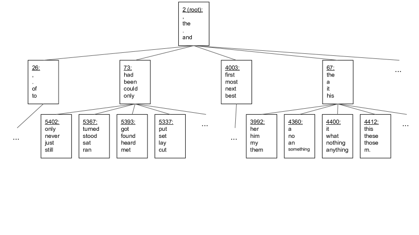
Figure 3: Tree learned from the Gutenberg corpus, showing the four most common words assigned to each node.

7 Experiments

We ran experiments to evaluate both the classification and density estimation version of our algorithm. For classification, we used the YFCC100M dataset (Thomee et al., 2016), which consists of a set of a hundred million Flickr pictures along with captions and tag sets split into 91M training, 930K validation and 543K test examples. We focus here on the problem of predicting a picture’s tags given its caption. For density estimation, we learned a log-bilinear language model on the Gutenberg novels corpus, and compared the perplexity to that obtained with other flat and hierarchical losses. Experimental settings are described in greater detail in the Supplementary material.

7.1 Classification

We follow the setting of (Joulin et al., 2016) for the YFCC100M tag prediction task: we only keep the tags which appear at least a hundred times, which leaves us with a label space of size 312K. We compare our results to those obtained with the FastText software (Joulin et al., 2016), which uses a binary hierarchical softmax objective based on Huffman coding (Huffman trees are designed to minimize the expected depth of their leaves weighed by frequencies and have been shown to work well with word embedding systems (Mikolov et al., 2013)), and to the Tagspace system (Weston et al., 2014), which uses a sampling-based margin loss (this allows for training in tractable time, but does not help at test time, hence the long times reported). We also extend the FastText software to use Huffman trees of arbitrary width. All models use a bag-of-word embedding representation of the caption text; the parameters of the input representation function $f_{\Theta}$ which we learn are the word embeddings $U_{w}\in\mathbb{R}^{d}$ (as in Section 6) and a caption representation is obtained by summing the embeddings of its words. We experimented with embeddings of dimension $d=50$ and $d=200$. We predict one tag for each caption, and report the precision as well as the training and test times in Table 1.

$d$	Model	Arity	P@1	Train	Test
50	TagSpace1	-	30.1	3h8	6h
	FastText2	2	27.2	8m	1m
	$M$-ary Huffman Tree	5	28.3	8m	1m
		20	29.9	10m	3m
	Learned Tree	5	31.6	18m	1m
		20	32.1	30m	3m
200	TagSpace1	35.6	5h32	15h
	FastText2	2	35.2	12m	1m
	$M$-ary Huffman Tree	5	35.8	13m	2m
		20	36.4	18m	3m
	Learned Tree	5	36.1	35m	3m
		20	36.6	45m	8m

Table 1: Classification performance on the YFCC100M dataset. ¹(Weston et al., 2014). ²(Joulin et al., 2016). $M$-ary Huffman Tree modifies FastText by adding an $M$-ary hierarchical softmax objective.

Our implementation is based on the FastText open source version, to which we added $M$-ary Huffman and learned tree objectives. Table 1 reports the best accuracy we obtained with a hyper-parameter search using this version on our system so as to provide the most meaningful comparison, even though the accuracy is less than that reported in (Joulin et al., 2016).

We gain a few different insights from Table 1. First, although wider trees are theoretically slower (remember that the theoretical complexity is $O(M\log_{M}(N))$ for an $M$-ary tree with $N$ labels), they run incomparable time in practice and always perform better. Using our algorithm to learn the structure of the tree also always leads to more accurate models, with a gain of up to 3.3 precision points in the smaller 5-ary setting. Further, both the importance of having wider trees and learning the structure seems to be less when the node prediction functions become more expressive. At a high level, one could imagine that in that setting, the model can learn to use different dimensions of the input representation for different nodes, which would minimize the negative impact of having to learn a representation which is suited to more nodes.

Another thing to notice is that since prediction time only depends on the expected depth of a label, our models which learned balanced trees are nearly as fast as Huffman coding which is optimal in that respect (except for the dimension 200, 20-ary tree, but the tree structure had not stabilized yet in that setting). Given all of the above remarks, our algorithm especially shines in settings where computational complexity and prediction time are highly constrained at test time, such as mobile devices or embedded systems.

7.2 Density Estimation

We also ran language modeling experiments on the Gutenberg novel corpus, which has about 50M tokens and a vocabulary of 250,000 words.

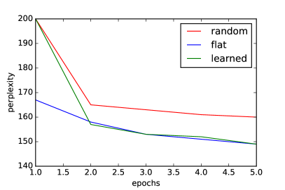
Figure 2: Test perplexity per epoch.

One notable difference from the previous task is that the language modeling setting can drastically benefit from the use of GPU computing, which can make using a flat softmax tractable (if not fast). While our algorithm requires more flexibility and thus does not benefit as much from the use of GPUs, a small modification of Algorithm 2 (described in the Supplementary material) allows it to run under a maximum depth constraint and remain competitive. The results presented in this section are obtained using this modified version, which learns 65-ary trees of depth 3.

Table 2 presents perplexity results for different loss functions, along with the time spent on computing and learning the objective (softmax parameters for the flat version, hierarchical softmax node parameters for the fixed tree, and hierarchical softmax structure and parameters for our algorithm). The learned tree model is nearly three and seven times as fast at train and test time respectively as the flat objective without losing any points of perplexity.

Model	perp.	train ms/batch	test ms/batch
Clustering Tree	212	2.0	1.0
Random Tree	160	1.9	0.9
Flat soft-max	149	12.5	6.9
Learned Tree	148	4.5	0.9

Table 2: Comparison of a flat soft-max to a 65-ary hierarchical soft-max (learned, random and heuristic-based tree).

Huffman coding does not apply to trees where all of the leaves are at the same depth. Instead, we use the following heuristic as a baseline, inspired by (Mnih & Hinton, 2009): we learn word embeddings using FastText, perform a hierarchical clustering of the vocabulary based on these, then use the resulting tree to learn a new language model. We call this approach “Clustering Tree”. However, for all hyper-parameter settings, this tree structure did worse than a random one. We conjecture that its poor performance is because such a tree structure means that the deepest node decisions can be quite difficult.

Figure 2 shows the evolution of the test perplexity for a few epochs. It appears that most of the relevant tree structure can be learned in one epoch: from the second epoch on, the learned hierarchical soft-max performs similarly to the flat one. Figure 3 shows a part of the tree learned on the Gutenberg dataset, which appears to make semantic and syntactic sense.

8 Conclusion

In this paper, we introduced a provably accurate algorithm for jointly learning tree structure and data representation for hierarchical prediction. We applied it to a multi-class classification and a density estimation problem, and showed our models’ ability to achieve favorable accuracy in competitive times in both settings.

9 Geometric interpretation of probabilities $\bm{p_{j}^{(n)}}$ and $\bm{p_{j|i}^{(n)}}$

Discrete:

$p_{1}^{(n)}=\frac{6}{12}=\bm{0.5}$

$p_{1|1}^{(n)}=\frac{3}{3}=\bm{1}$,      $p_{1|2}^{(n)}=\frac{3}{3}=\bm{1}$,      $p_{1|3}^{(n)}=\frac{0}{3}=\bm{0}$,      $p_{1|4}^{(n)}=\frac{0}{3}=\bm{0}$

Continuous:

$p_{1}^{(n)}=\frac{1}{12}(\sigma(100)+\sigma(70)+\ldots+\sigma(-70)+\sigma(-100))\approx\bm{0.5}$

$p_{1|1}^{(n)}=\frac{1}{3}(\sigma(100)+\sigma(70)+\sigma(100))\approx\bm{1}$

$p_{1|2}^{(n)}=\frac{1}{3}(\sigma(100)+\sigma(70)+\sigma(100))\approx\bm{1}$

$p_{1|3}^{(n)}=\frac{1}{3}(\sigma(-100)+\sigma(-70)+\sigma(-100))\approx\bm{0}$

$p_{1|4}^{(n)}=\frac{1}{3}(\sigma(-100)+\sigma(-70)+\sigma(-100))\approx\bm{0}$

Figure 3: The comparison of discrete and continuous definitions of probabilities $p_{j}^{(n)}$ and $p_{j|i}^{(n)}$ on a simple example with $K=4$ classes and binary tree ($M=2$). $n$ is an exemplary node, e.g. root. $\sigma$ denotes sigmoid function. Color circles denote data points.

Remark 3.

One could define $p_{j}^{(n)}$ as the ratio of the number of examples that reach node $n$ and are sent to its $j^{\text{th}}$ child to the total the number of examples that reach node $n$ and $p_{j|i}^{(n)}$ as the ratio of the number of examples that reach node $n$, correspond to label $i$, and are sent to the $j^{\text{th}}$ child of node $n$ to the total the number of examples that reach node $n$ and correspond to label $i$. We instead look at the continuous counter-parts of these discrete definitions as given by Equations 8 and 9 and illustrated in Figure 3 (note that continuous definitions have elegant geometric interpretation based on margins), which simplifies the optimization problem.

10 Theoretical proofs

Proof of Lemma 1.

Recall the form of the objective defined in 6:

$$J_{n} = \frac{2}{M}\sum_{i=1}^{K}q^{(n)}_{i}\Big{(}\sum_{j=1}^{M}|p^{(n)}_{j}-p^{(n)}_{j|i}|\Big{)}$$

$$= \frac{2}{M}{\mathbb{E}}_{i\sim q^{(n)}}\Big{[}f^{J}_{n}(i,p^{(n)}_{\cdot|\cdot},q^{(n)})\Big{]}$$

Where:

$$f^{J}_{n}(i,p^{(n)}_{\cdot|\cdot},q^{(n)}) = \sum_{j=1}^{M}\Big{|}p^{(n)}_{j}-p^{(n)}_{j|i}\Big{|}=\sum_{j=1}^{M}\Big{|}p^{(n)}_{j|i}-\sum_{i^{\prime}=1}^{K}q^{(n)}_{i^{\prime}}p^{(n)}_{j|i^{\prime}}\Big{|}$$

$$= \sum_{j=1}^{M}\Big{|}\sum_{i^{\prime}=1}^{K}({\mathbbm{1}}_{i=i^{\prime}}-q^{(n)}_{i^{\prime}})p^{(n)}_{j|i^{\prime}}\Big{|}$$

Hence:

$$\frac{\partial f^{J}_{n}(i,p^{(n)}_{\cdot|\cdot},q^{(n)})}{\partial p^{(n)}_{j|i}}=(1-q^{(n)}_{i})\operatorname{sign}(p^{(n)}_{j|i}-p^{(n)}_{j})$$

And:

$$\frac{\partial f^{J}_{n}(i,p^{(n)}_{\cdot|\cdot},q^{(n)})}{\partial\log p^{(n)}_{j|i}} = (1-q^{(n)}_{i})\operatorname{sign}(p^{(n)}_{j|i}-p^{(n)}_{j})\frac{\partial p^{(n)}_{j|i}}{\partial\log p^{(n)}_{j|i}}$$

$$= (1-q^{(n)}_{i})\operatorname{sign}(p^{(n)}_{j|i}-p^{(n)}_{j})p^{(n)}_{j|i}$$

By assigning each label $j$ to a specific child $i$ under the constraint that no child has more than $L$ labels, we take a step in the direction $\partial E\in\{0,1\}^{M\times K}$, where:

$$\forall i\in[1,K], \sum_{j=1}^{M}\partial E_{j,i}=1$$

and

$$\forall j\in[1,M], \sum_{i=1}^{K}\partial E_{j,i}\leq L$$

Thus:

$$\frac{\partial J_{n}}{\partial p_{\cdot|\cdot}^{(n)}}\partial E = \frac{2}{M}\frac{{\mathbb{E}}_{i\sim q^{(n)}}\Big{[}f^{J}_{n}(i,p^{(n)}_{\cdot|\cdot},q^{(n)})\Big{]}}{\partial p_{\cdot|\cdot}^{(n)}}\partial E$$ (13)

$$= \frac{2}{M}\sum_{i=1}^{K}q_{i}^{(n)}(1-q_{i}^{(n)})\sum_{j=1}^{M}\Big{(}\operatorname{sign}(p^{(n)}_{j|i}-p^{(n)}_{j})\partial E_{j,i}\Big{)}$$

And:

$$\frac{\partial J_{n}}{\partial\log p_{\cdot|\cdot}^{(n)}}\partial E=\frac{2}{M}\sum_{i=1}^{K}q_{i}^{(n)}(1-q_{i}^{(n)})\sum_{j=1}^{M}\Big{(}\operatorname{sign}(p^{(n)}_{j|i}-p^{(n)}_{j})p^{(n)}_{j|i}\partial E_{j,i}\Big{)}$$ (14)

If there exists such an assignment for which 13 is positive, then the greedy method proposed in 2 finds it. Indeed, suppose that Algorithm 2 assigns label $i$ to child $j$ and $i^{\prime}$ to $j^{\prime}$. Suppose now that another assignment $\partial E^{\prime}$ sends $i$ to $j^{\prime}$ and $i$ to $j^{\prime}$. Then:

$$\frac{\partial J_{n}}{\partial p_{\cdot|\cdot}^{(n)}}\Big{(}\partial E-\partial E^{\prime}\Big{)}=\Big{(}\frac{\partial J_{n}}{\partial p_{j|i}^{(n)}}+\frac{\partial J_{n}}{\partial p_{j^{\prime}|i^{\prime}}^{(n)}}\Big{)}-\Big{(}\frac{\partial J_{n}}{\partial p_{j|i^{\prime}}^{(n)}}+\frac{\partial J_{n}}{\partial p_{j^{\prime}|i}^{(n)}}\Big{)}$$ (15)

Since the algorithm assigns children by descending order of $\frac{\partial J_{n}}{\partial p_{j|i}^{(n)}}$ until a child $j$ is full, we have:

$$\frac{\partial J_{n}}{\partial p_{j|i}^{(n)}}\geq\frac{\partial J_{n}}{\partial p_{j|i^{\prime}}^{(n)}}\;\;\;\;\;\;\text{and}\;\;\;\;\;\;\frac{\partial J_{n}}{\partial p_{{}^{\prime}j|i^{\prime}}^{(n)}}\geq\frac{\partial J_{n}}{\partial p_{j^{\prime}|i}^{(n)}}$$

Hence:

$$\frac{\partial J_{n}}{\partial p_{\cdot|\cdot}^{(n)}}\Big{(}\partial E-\partial E^{\prime}\Big{)}\geq 0$$

Thus, the greedy algorithm finds the assignment that most increases $J_{n}$ most under the children size constraints.

Moreover, $\frac{\partial J_{n}}{\partial p_{\cdot|\cdot}^{(n)}}$ is always positive for $L\leq M$ or $L\geq 2M(M-2)$. ∎

Proof of Lemma 2.

Both $J_{n}$ and $J_{T}$ are defined as the sum of non-negative values which gives the lower-bound. We next derive the upper-bound on $J_{n}$. Recall:

$$J_{n}=\frac{2}{M}\sum_{j=1}^{M}\sum_{i=1}^{K}q^{(n)}_{i}|p_{j}^{(n)}-p^{(n)}_{j|i}|=\frac{2}{M}\sum_{j=1}^{M}\sum_{i=1}^{K}q^{(n)}_{i}\left|\sum_{l=1}^{K}q^{(n)}_{l}p^{(n)}_{j|l}-p^{(n)}_{j|i}\right|$$

since $p_{j}^{(n)}=\sum_{l=1}^{K}q^{(n)}_{l}p^{(n)}_{j|l}$. The objective $J_{n}$ is maximized on the extremes of the $[0,1]$ interval. Thus, define the following two sets of indices:

$$O_{j}=\{i:i\in\{1,2,\dots,K\},p^{(n)}_{j|i}=1\}\text{\>\>\>\>\>\>\>and\>\>\>\>\>\>\>}Z_{j}=\{i:i\in\{1,2,\dots,K\},p^{(n)}_{j|i}=0\}.$$

We omit indexing these sets with $n$ for the ease of notation. We continue as follows

$$J_{n} \leq \frac{2}{M}\sum_{j=1}^{M}\left[\sum_{i\in O_{j}}q^{(n)}_{i}\left(1-\sum_{l\in O_{j}}q^{(n)}_{l}\right)+\sum_{i\in Z_{j}}q^{(n)}_{i}\sum_{l\in O_{j}}q^{(n)}_{l}\right]$$

$$= \frac{4}{M}\sum_{j=1}^{M}\left[\sum_{i\in O_{j}}q^{(n)}_{i}-\left(\sum_{i\in O_{j}}q^{(n)}_{i}\right)^{2}\right]$$

$$= \frac{4}{M}\left[1-\sum_{j=1}^{M}\left(\sum_{i\in O_{j}}q^{(n)}_{i}\right)^{2}\right],$$

where the last inequality is the consequence of the following: $\sum_{j=1}^{M}p^{(n)}_{j}=1$ and $p^{(n)}_{j}=\sum_{l=1}^{K}q_{l}^{(n)}p^{(n)}_{j|l}=\sum_{i\in O_{j}}q^{(n)}_{i}$, thus $\sum_{j=1}^{M}\sum_{i\in O_{j}}q^{(n)}_{i}=1$. Apllying Jensen’s ineqality to the last inequality obtained gives

$$J_{n} \leq \frac{4}{M}-4\left[\sum_{j=1}^{M}\left(\frac{1}{M}\sum_{i\in O_{j}}q^{(n)}_{i}\right)\right]^{2}$$

$$= \frac{4}{M}\left(1-\frac{1}{M}\right)$$

That ends the proof. ∎

Proof of Lemma 3.

We start from proving that if the split in node $n$ is perfectly balanced, i.e. $\forall_{j=\{1,2,\dots,M\}}p^{(n)}_{j}=\frac{1}{M}$, and perfectly pure, i.e. $\forall_{\begin{subarray}{c}j=\{1,2,\dots,M\}\\ i=\{1,2,\dots,K\}\end{subarray}}\min(p^{(n)}_{j|i},1-p^{(n)}_{j|i})=0$, then $J_{n}$ admits the highest value $J_{n}=\frac{4}{M}\left(1-\frac{1}{M}\right)$. Since the split is maximally balanced we write:

$$J_{n}=\frac{2}{M}\sum_{j=1}^{M}\sum_{i=1}^{K}q^{(n)}_{i}\left|\frac{1}{M}-p^{(n)}_{j|i}\right|.$$

Since the split is maximally pure, each $p^{(n)}_{j|i}$ can only take value $0$ or $1$. As in the proof of previous lemma, define two sets of indices:

$$O_{j}=\{i:i\in\{1,2,\dots,K\},p^{(n)}_{j|i}=1\}\text{\>\>\>\>\>\>\>and\>\>\>\>\>\>\>}Z_{j}=\{i:i\in\{1,2,\dots,K\},p^{(n)}_{j|i}=0\}.$$

We omit indexing these sets with $n$ for the ease of notation. Thus

$$J_{n} = \frac{2}{M}\sum_{j=1}^{M}\left[\sum_{i\in O_{j}}q^{(n)}_{i}\left(1-\frac{1}{M}\right)+\sum_{i\in Z_{j}}q^{(n)}_{i}\frac{1}{M}\right]$$

$$= \frac{2}{M}\sum_{j=1}^{M}\left[\sum_{i\in O_{j}}q^{(n)}_{i}\left(1-\frac{1}{M}\right)+\frac{1}{M}\left(1-\sum_{i\in O_{j}}q^{(n)}_{i}\right)\right]$$

$$= \frac{2}{M}\left(1-\frac{2}{M}\right)\sum_{j=1}^{M}\sum_{i\in O_{j}}q^{(n)}_{i}+\frac{2}{M}$$

$$= \frac{4}{M}\left(1-\frac{1}{M}\right),$$

where the last equality comes from the fact that $\sum_{j=1}^{M}p^{(n)}_{j}=1$ and $p^{(n)}_{j}=\sum_{l=1}^{K}q^{(n)}_{l}p^{(n)}_{j|l}=\sum_{i\in O_{j}}q^{(n)}_{i}$, thus $\sum_{j=1}^{M}\sum_{i\in O_{j}}q^{(n)}_{i}=1$.

Thus we are done with proving one induction direction. Next we prove that if $J_{n}$ admits the highest value $J_{n}=\frac{4}{M}\left(1-\frac{1}{M}\right)$, then the split in node $n$ is perfectly balanced, i.e. $\forall_{j=\{1,2,\dots,M\}}p^{(n)}_{j}=\frac{1}{M}$, and perfectly pure, i.e. $\forall_{\begin{subarray}{c}j=\{1,2,\dots,M\}\\ i=\{1,2,\dots,K\}\end{subarray}}\min(p^{(n)}_{j|i},1-p^{(n)}_{j|i})=0$.

Without loss of generality assume each $q^{(n)}_{i}\in(0,1)$. The objective $J_{n}$ is certainly maximized in the extremes of the interval $[0,1]$, where each $p^{(n)}_{j|i}$ is either $0$ or $1$. Also, at maximum it cannot be that for any given $j$, all $p^{(n)}_{j|i}$’s are $0$ or all $p^{(n)}_{j|i}$’s are $1$. The function $J(h)$ is differentiable in these extremes. Next, define three sets of indices:

$$\mathcal{A}_{j}=\{i:\sum_{l=1}^{K}q^{(n)}_{i}p^{(n)}_{j|l}\geq p^{(n)}_{j|i}\}\text{\>\>\>\>\>\>\>and\>\>\>\>\>\>\>}\mathcal{B}_{j}=\{i:\sum_{l=1}^{K}q^{(n)}_{i}p^{(n)}_{j|l}<p^{(n)}_{j|i}\}\text{\>\>\>\>\>\>\>and\>\>\>\>\>\>\>}\mathcal{C}_{j}=\{i:\sum_{l=1}^{K}q^{(n)}_{i}p^{(n)}_{j|l}>p^{(n)}_{j|i}\}.$$

We omit indexing these sets with $n$ for the ease of notation. Objective $J_{n}$ can then be re-written as

$$J_{n}=\frac{2}{M}\sum_{j=1}^{M}\left[\sum_{i\in\mathcal{A}_{j}}q^{(n)}_{i}\left(\sum_{l=1}^{K}q^{(n)}_{i}p^{(n)}_{j|l}-p^{(n)}_{j|i}\right)+2\sum_{i\in\mathcal{B}_{j}}q^{(n)}_{i}\left(p^{(n)}_{j|i}-\sum_{l=1}^{K}q^{(n)}_{i}p^{(n)}_{j|l}\right)\right],$$

We next compute the derivatives of $J_{n}$ with respect to $p^{(n)}_{j|z}$, where $z=\{1,2,\dots,K\}$, everywhere where the function is differentiable and obtain

$$\frac{\partial J_{n}}{\partial p^{(n)}_{j|z}}=\left\{\begin{tabular}[]{c}$2q^{(n)}_{z}(\sum_{i\in\mathcal{C}_{j}}q^{(n)}_{i}-1)\>\>\>\>\>$ if$\>$$z\in\mathcal{C}_{j}$\\ $\>2q^{(n)}_{z}(1-\sum_{i\in\mathcal{B}_{j}}q^{(n)}_{i})\>\>\>\>$ if$\>$$z\in\mathcal{B}_{j}$\end{tabular}\right.,$$

Note that in the extremes of the interval $[0,1]$ where $J_{n}$ is maximized, it cannot be that $\sum_{i\in\mathcal{C}_{j}}q^{(n)}_{i}=1$ or $\sum_{i\in\mathcal{B}_{j}}q^{(n)}_{i}=1$ thus the gradient is non-zero. This fact and the fact that $J_{n}$ is convex imply that $J_{n}$ can only be maximized at the extremes of the $[0,1]$ interval. Thus if $J_{n}$ admits the highest value, then the node split is perfectly pure. We still need to show that if $J_{n}$ admits the highest value, then the node split is also perfectly balanced. We give a proof by contradiction, thus we assume that at least for one value of $j$, $p^{(n)}_{j}\neq\frac{1}{M}$, or in other words if we decompose each $p^{(n)}_{j}$ as $p^{(n)}_{j}=\frac{1}{M}+x_{j}$, then at least for one value of $j$, $x_{j}\neq 0$. Lets once again define two sets of indices (we omit indexing $x_{j}$ and these sets with $n$ for the ease of notation):

$$O_{j}=\{i:i\in\{1,2,\dots,K\},p^{(n)}_{j|i}=1\}\text{\>\>\>\>\>\>\>and\>\>\>\>\>\>\>}Z_{j}=\{i:i\in\{1,2,\dots,K\},p^{(n)}_{j|i}=0\},$$

and recall that $p^{(n)}_{j}=\sum_{l=1}^{K}q^{(n)}_{l}p^{(n)}_{j|l}=\sum_{i\in O_{j}}q^{(n)}_{i}$. We proceed as follows

$$\frac{4}{M}\left(1-\frac{1}{M}\right)=J_{n} = \frac{2}{M}\sum_{j=1}^{M}\left[\sum_{i\in O_{j}}q^{(n)}_{i}(1-p^{(n)}_{j})+\sum_{i\in Z_{j}}q^{(n)}_{i}p^{(n)}_{j}\right]$$

$$= \frac{2}{M}\sum_{j=1}^{M}\left[p^{(n)}_{j}(1-p^{(n)}_{j})+p^{(n)}_{j}(1-p^{(n)}_{j})\right]$$

$$= \frac{4}{M}\sum_{j=1}^{M}\left[p^{(n)}_{j}-(p^{(n)}_{j})^{2}\right]$$

$$= \frac{4}{M}\left[1-\sum_{j=1}^{M}(p^{(n)}_{j})^{2}\right]$$

$$= \frac{4}{M}\left[1-\sum_{j=1}^{M}\left(\frac{1}{M}+x_{j}\right)^{2}\right]$$

$$= \frac{4}{M}\left(1-\frac{1}{M}-\frac{2}{M}\sum_{j=1}^{M}x_{j}-\sum_{j=1}^{M}x_{j}^{2}\right)$$

$$< \frac{4}{M}\left(1-\frac{1}{M}\right)$$

Thus we obtain the contradiction which ends the proof. ∎

Proof of Lemma 4.

Since we node that the split is perfectly pure, then each $p_{j|i}^{(n)}$ is either $0$ or $1$. Thus we define two sets

$$O_{j}=\{i:i\in\{1,2,\dots,K\},p^{(n)}_{j|i}=1\}\text{\>\>\>\>\>\>\>and\>\>\>\>\>\>\>}Z_{j}=\{i:i\in\{1,2,\dots,K\},p^{(n)}_{j|i}=0\}.$$

and thus

$$J_{n}=\frac{2}{M}\sum_{j=1}^{M}\left[\sum_{i\in O_{j}}q^{(n)}_{i}\left(1-p_{j}\right)+\sum_{i\in Z_{j}}q^{(n)}_{i}p_{j}\right]$$

Note that $p_{j}=\sum_{i\in O_{j}}q_{i}^{(n)}$. Then

$$J_{n}=\frac{2}{M}\sum_{j=1}^{M}\left[p_{j}\left(1-p_{j}\right)+(1-p_{j})p_{j}\right]=\frac{4}{M}\sum_{j=1}^{M}p_{j}\left(1-p_{j}\right)=\frac{4}{M}\left(1-\sum_{j=1}^{M}p_{j}^{2}\right)$$

and thus

$$\sum_{j=1}^{M}p_{j}^{2}=1-\frac{MJ_{n}}{4}.$$ (16)

Lets express $p_{j}$ as $p_{j}=\frac{1}{M}+\epsilon_{j}$, where $\epsilon_{j}\in[-\frac{1}{M},1-\frac{1}{M}]$. Then

$$\sum_{j=1}^{M}p_{j}^{2}=\sum_{j=1}^{M}\left(\frac{1}{M}+\epsilon_{j}\right)^{2}=\frac{1}{M}+\frac{2}{M}\sum_{j=1}^{M}\epsilon_{j}+\sum_{j=1}^{M}\epsilon_{j}^{2}=\frac{1}{M}+\sum_{j=1}^{M}\epsilon_{j}^{2},$$ (17)

since $\frac{2}{M}\sum_{j=1}^{M}\epsilon_{j}=0$. Thus combining Equation 16 and 17

$$\frac{1}{M}+\sum_{j=1}^{M}\epsilon_{j}^{2}=1-\frac{MJ_{n}}{4}$$

and thus

$$\sum_{j=1}^{M}\epsilon_{j}^{2}=1-\frac{1}{M}-\frac{MJ_{n}}{4}.$$

The last statement implies that

$$\max_{j=1,2,\dots,M}\epsilon_{j}\leq\sqrt{1-\frac{1}{M}-\frac{MJ_{n}}{4}},$$

which is equivalent to

$$\min_{j=1,2,\dots,M}p_{j}=\frac{1}{M}-\max_{j}\epsilon_{j}\geq\frac{1}{M}-\sqrt{1-\frac{1}{M}-\frac{MJ_{n}}{4}}=\frac{1}{M}-\frac{\sqrt{M(J^{*}-J_{n})}}{2}.$$

∎

Proof of Lemma 5.

Since the split is perfectly balanced we have the following:

$$J_{n}=\frac{2}{M}\sum_{j=1}^{M}\sum_{i=1}^{K}q_{i}^{(n)}\left|\frac{1}{M}-p_{j|i}^{(n)}\right|=\frac{2}{M}\sum_{i=1}^{K}\sum_{j=1}^{M}q_{i}^{(n)}\left|\frac{1}{M}-p_{j|i}^{(n)}\right|$$

Define two sets

$$\mathcal{A}_{i}=\{j:j\in\{1,2,\dots,K\},p^{(n)}_{j|i}<\frac{1}{M}\}\text{\>\>\>\>\>\>\>and\>\>\>\>\>\>\>}\mathcal{B}_{i}=\{j:j\in\{1,2,\dots,K\},p^{(n)}_{j|i}\geq\frac{1}{M}\}.$$

Then

$$J_{n} = \frac{2}{M}\sum_{i=1}^{K}\left[\sum_{j\in\mathcal{A}_{i}}q_{i}^{(n)}\left(\frac{1}{M}-p_{j|i}^{(n)}\right)+\sum_{j\in\mathcal{B}_{i}}q_{i}^{(n)}\left(p_{j|i}^{(n)}-\frac{1}{M}\right)\right]$$

$$= \frac{2}{M}\sum_{i=1}^{K}q_{i}^{(n)}\left[\sum_{j\in\mathcal{A}_{i}}\left(\frac{1}{M}-p_{j|i}^{(n)}\right)+\sum_{j\in\mathcal{B}_{i}}\left(p_{j|i}^{(n)}-\frac{1}{M}\right)\right]$$

$$= \frac{2}{M}\sum_{i=1}^{K}q_{i}^{(n)}\left[\sum_{j\in\mathcal{A}_{i}}\left(\frac{1}{M}-p_{j|i}^{(n)}\right)+\sum_{j\in\mathcal{B}_{i}}\left((1-\frac{1}{M})-(1-p_{j|i}^{(n)})\right)\right]$$

Recall that the optimal value of $J_{n}$ is:

$$J^{*}=\frac{4}{M}\left(1-\frac{1}{M}\right)=\frac{2}{M}\sum_{i=1}^{N}q_{i}^{(n)}\left[\left(M-1\right)\frac{1}{M}+\left(1-\frac{1}{M}\right)\right]=\frac{2}{M}\sum_{i=1}^{N}q_{i}^{(n)}\left[\left(\sum_{j\in\mathcal{A}_{i}\cup\mathcal{B}_{i}}\frac{1}{M}\right)-\frac{1}{M}+\left(1-\frac{1}{M}\right)\right]$$

Note $\mathcal{A}_{i}$ can have at most $M-1$ elements. Furthermore, $\forall j\in\mathcal{A}_{i},p_{j|i}^{(n)}<1-p_{j|i}^{(n)}$. Then, we have:

$$J^{*}-J^{n}=\frac{2}{M}\sum_{i=1}^{K}q_{i}^{(n)}\left[\sum_{j\in\mathcal{A}_{i}}p_{j|i}^{(n)}+\sum_{j\in\mathcal{B}_{i}}\left((1-p_{j|i}^{(n)})+\frac{1}{M}-(1-\frac{1}{M})\right)-\frac{1}{M}+\left(1-\frac{1}{M}\right)\right]$$

Hence, since $\mathcal{B}_{i}$ has at least one element:

$$J^{*}-J^{n} \geq \frac{2}{M}\sum_{i=1}^{K}q_{i}^{(n)}\left[\sum_{j\in\mathcal{A}_{i}}p_{j|i}^{(n)}+\sum_{j\in\mathcal{B}_{i}}\left(1-p_{j|i}^{(n)}\right)\right]$$

$$\geq \frac{2}{M}\sum_{i=1}^{K}q_{i}^{(n)}\left[\sum_{j=1}^{M}\min(p_{j|i}^{(n)},1-p_{j|i}^{(n)})\right]$$

$$\geq 2\alpha$$

∎

Proof of Theorem 1.

Let the weight of the tree leaf be defined as the probability that a randomly chosen data point $x$ drawn from some fixed target distribution $\mathcal{P}$ reaches this leaf. Suppose at time step $t$, $n$ is the heaviest leaf and has weight $w$. Consider splitting this leaf to $M$ children $n_{1},n_{2},\dots,n_{M}$. Let the weight of the $j^{\text{th}}$ child be denoted as $w_{j}$. Also for the ease of notation let $p_{j}$ refer to $p_{j}^{(n)}$ (recall that $\sum_{j=1}^{m}p_{j}=1$) and $p_{j|i}$ refer to $p_{j|i}^{(n)}$, and furthermore let $q_{i}$ be the shorthand for $q^{(n)}_{i}$. Recall that $p_{j}=\sum_{i=1}^{K}q_{i}p_{j|i}$ and $\sum_{i=1}^{K}q_{i}=1$. Notice that for any $j=\{1,2,\dots,M\}$, $w_{j}=wp_{j}$. Let ${\bm{q}}$ be the $k$-element vector with $i^{th}$ entry equal to $q_{i}$. Define the following function: $\tilde{G}^{e}({\bm{q}})=\sum_{i=1}^{K}q_{i}\ln\left(\frac{1}{q_{i}}\right)$. Recall the expression for the entropy of tree leaves: $G^{e}=\sum_{l\in\mathcal{L}}w_{l}\sum_{i=1}^{K}q^{(l)}_{i}\ln\left(\frac{1}{q^{(l)}_{i}}\right)$, where $\mathcal{L}$ is a set of all tree leaves. Before the split the contribution of node $n$ to $G^{e}$ was equal to $w\tilde{G}^{e}({\bm{q}})$. Note that for any $j=\{1,2,\dots,M\}$, $q^{(n_{j})}_{i}=\frac{q_{i}p_{j|i}}{p_{j}}$ is the probability that a randomly chosen $x$ drawn from $\mathcal{P}$ has label $i$ given that $x$ reaches node $n_{j}$. For brevity, let $q^{n^{j}}_{i}$ be denoted as $q_{j,i}$. Let ${\bm{q}}_{j}$ be the $k$-element vector with $i^{th}$ entry equal to $q_{j,i}$. Notice that ${\bm{q}}=\sum_{j=1}^{M}p_{j}{\bm{q}}_{j}$. After the split the contribution of the same, now internal, node $n$ changes to $w\sum_{j=1}^{M}p_{j}\tilde{G}^{e}({\bm{q}}_{j})$. We denote the difference between the contribution of node $n$ to the value of the entropy-based objectives in times $t$ and $t+1$ as

$$\Delta_{t}^{e}:=G_{t}^{e}-G_{t+1}^{e}=w\left[\tilde{G}^{e}({\bm{q}})-\sum_{j=1}^{M}p_{j}\tilde{G}^{e}({\bm{q}}_{j})\right].$$ (18)

The entropy function $\tilde{G}^{e}$ is strongly concave with respect to $l_{1}$-norm with modulus $1$, thus we extend the inequality given by Equation 7 in (Choromanska et al., 2016) by applying Theorem 5.2. from (Azocar et al., 2011) and obtain the following bound

$$\Delta_{t}^{e} = w\left[\tilde{G}^{e}({\bm{q}})-\sum_{j=1}^{M}p_{j}\tilde{G}^{e}({\bm{q}}_{j})\right]$$

$$\geq w\frac{1}{2}\sum_{j=1}^{M}p_{j}\|q_{j}-\sum_{l=1}^{M}p_{l}q_{l}\|_{1}^{2}$$

$$= w\frac{1}{2}\sum_{j=1}^{M}p_{j}\left(\sum_{i=1}^{K}\left|\frac{q_{i}p_{j|i}}{p_{j}}-\sum_{l=1}^{M}p_{l}\frac{q_{i}p_{l|i}}{p_{l}}\right|\right)^{2}$$

$$= w\frac{1}{2}\sum_{j=1}^{M}p_{j}\left(\sum_{i=1}^{K}q_{i}\left|\frac{p_{j|i}}{p_{j}}-\sum_{l=1}^{M}p_{l|i}\right|\right)^{2}$$

$$= w\frac{1}{2}\sum_{j=1}^{M}p_{j}\left(\sum_{i=1}^{K}q_{i}\left|\frac{p_{j|i}}{p_{j}}-1\right|\right)^{2}$$

$$= w\frac{1}{2}\sum_{j=1}^{M}\frac{1}{p_{j}}\left(\sum_{i=1}^{K}q_{i}\left|p_{j|i}-p_{j}\right|\right)^{2}.$$

Before proceeding, we will bound each $p_{j}$. Note that by the Weak Hypothesis Assumption we have

$$\gamma\in\left[\frac{M}{2}\min_{j=1,2,\dots,M}p_{j},1-\frac{M}{2}\min_{j=1,2,\dots,M}p_{j}\right],$$

thus

$$\min_{j=1,2,\dots,M}p_{j}\geq\frac{2\gamma}{M},$$

thus all $p_{j}$s are such that $p_{j}\geq\frac{2\gamma}{M}$. Thus

$$\max_{j=1,2,\dots,M}p_{j}\leq 1-\frac{2\gamma}{M}(M-1)=\frac{M(1-2\gamma)+2\gamma}{M}.$$

Thus all $p_{j}$s are such that $p_{j}\leq\frac{M(1-2\gamma)+2\gamma}{M}$.

$$\Delta_{t}^{e} \geq w\frac{M^{2}}{2[(M(1-2\gamma)+2\gamma]}\sum_{j=1}^{M}\frac{1}{M}\left(\sum_{i=1}^{K}q_{i}\left|p_{j|i}-p_{j}\right|\right)^{2}$$

$$\geq w\frac{M^{2}}{2[(M(1-2\gamma)+2\gamma]}\left(\sum_{j=1}^{M}\frac{1}{M}\sum_{i=1}^{K}q_{i}\left|p_{j|i}-p_{j}\right|\right)^{2}$$

$$= w\frac{M^{2}}{8[(M(1-2\gamma)+2\gamma]}\left(\frac{2}{M}\sum_{j=1}^{M}\sum_{i=1}^{K}q_{i}\left|p_{j|i}-p_{j}\right|\right)^{2}$$

$$= \frac{M^{2}}{[(M(1-2\gamma)+2\gamma]}\frac{wJ_{n}^{2}}{8},$$

where the last inequality is a consequence of Jensen’s inequality. $w$ can further be lower-bounded by noticing the following

$$G^{e}_{t}=\sum_{l\in\mathcal{L}}w_{l}\sum_{i=1}^{K}q^{(l)}_{i}\ln\left(\frac{1}{q^{(l)}_{i}}\right)\leq\sum_{l\in\mathcal{L}}w_{l}\ln K\leq w\ln K\sum_{l\in\mathcal{L}}1=[t(M-1)+1]w\ln K\leq(t+1)(M-1)w\ln K,$$

where the first inequality results from the fact that uniform distribution maximizes the entropy.

This gives the lower-bound on $\Delta_{t}^{e}$ of the following form:

$$\Delta_{t}^{e}\geq\frac{M^{2}G^{e}_{t}J_{n}^{2}}{8(t+1)[M(1-2\gamma)+2\gamma](M-1)\ln K},$$

and by using Weak Hypothesis Assumption we get

$$\Delta_{t}^{e}\geq\geq\frac{M^{2}G^{e}_{t}\gamma^{2}}{8(t+1)[M(1-2\gamma)+2\gamma](M-1)\ln K}$$

Following the recursion of the proof in Section 3.2 in (Choromanska et al., 2016) (note that in our case $G^{e}_{1}\leq 2(M-1)\ln K$), we obtain that under the Weak Hypothesis Assumption, for any $\kappa\in[0,2(M-1)\ln K]$, to obtain $G_{t}^{e}\leq\kappa$ it suffices to make

$$t\geq\left(\frac{2(M-1)\ln K}{\kappa}\right)^{\frac{16[M(1-2\gamma)+2\gamma](M-1)\ln K}{M^{2}\log_{2}e\gamma^{2}}}$$

splits. We next proceed to directly proving the error bound. Denote $w(l)$ to be the probability that a data point $x$ reached leaf $l$. Recall that $q^{(l)}_{i}$ is the probability that the data point $x$ corresponds to label $i$ given that $x$ reached $l$, i.e. $q^{(l)}_{i}=P(y(x)=i|x\>\>\text{reached}\>\>l)$. Let the label assigned to the leaf be the majority label and thus lets assume that the leaf is assigned to label $i$ if and only if the following is true $\forall_{\begin{subarray}{c}z=\{1,2,\dots,k\}\\ z\neq i\end{subarray}}q^{(l)}_{i}\geq q^{(l)}_{z}$. Therefore we can write that

$$\!\!\!\!\!\!\!\!\epsilon(\mathcal{T})\!\!\!\! = \!\!\!\!\sum_{i=1}^{K}P(t(x)=i,y(x)\neq i)$$

$$= \sum_{l\in\mathcal{L}}w(l)\sum_{i=1}^{K}P(t(x)=i,y(x)\neq i|x\>\>\text{reached}\>\>l)$$

$$= \sum_{l\in\mathcal{L}}w(l)\sum_{i=1}^{K}P(y(x)\neq i|t(x)=i,x\>\>\text{reached}\>\>l)P(t(x)=i|x\>\>\text{reached}\>\>l)$$

$$= \sum_{l\in\mathcal{L}}w(l)(1-\max(q^{(l)}_{1},q^{(l)}_{2},\dots,q^{(l)}_{K}))\sum_{i=1}^{K}P(t(x)=i|x\>\>\text{reached}\>\>l)$$

$$= \sum_{l\in\mathcal{L}}w(l)(1-\max(q^{(l)}_{1},q^{(l)}_{2},\dots,q^{(l)}_{K}))$$ (20)

Consider again the Shannon entropy $G(\mathcal{T})$ of the leaves of tree $\mathcal{T}$ that is defined as

$$G^{e}(\mathcal{T})=\sum_{l\in\mathcal{L}}w(l)\sum_{i=1}^{K}q^{(l)}_{i}\log_{2}\frac{1}{q^{(l)}_{i}}.$$ (21)

Let $i_{l}=\arg\max_{i=\{1,2,\dots,K\}}q^{(l)}_{i}$. Note that

$$G^{e}(\mathcal{T}) = \sum_{l\in\mathcal{L}}w(l)\sum_{i=1}^{K}q^{(l)}_{i}\log_{2}\frac{1}{q^{(l)}_{i}}$$ (22)

$$\geq \sum_{l\in\mathcal{L}}w(l)\sum_{\begin{subarray}{c}i=1\\ i\neq i_{l}\end{subarray}}^{K}q^{(l)}_{i}\log_{2}\frac{1}{q^{(l)}_{i}}$$

$$\geq \sum_{l\in\mathcal{L}}w(l)\sum_{\begin{subarray}{c}i=1\\ i\neq i_{l}\end{subarray}}^{K}q^{(l)}_{i}$$

$$= \sum_{l\in\mathcal{L}}w(l)(1-\max(q^{(l)}_{1},q^{(l)}_{2},\dots,q^{(l)}_{K}))$$

$$= \epsilon(\mathcal{T}),$$

where the last inequality comes from the fact that $\forall_{\begin{subarray}{c}i=\{1,2,\dots,K\}\\ i\neq i_{l}\end{subarray}}q^{(l)}_{i}\leq 0.5$ and thus $\forall_{\begin{subarray}{c}i=\{1,2,\dots,K\}\\ i\neq i_{l}\end{subarray}}\frac{1}{q^{(l)}_{i}}\in[2;+\infty]$ and consequently $\forall_{\begin{subarray}{c}i=\{1,2,\dots,K\}\\ i\neq i_{l}\end{subarray}}\log_{2}\frac{1}{q^{(l)}_{i}}\in[1;+\infty]$.

We next use the proof of Theorem 6 in (Choromanska et al., 2016). The proof modifies only slightly for our purposes and thus we only list these modifications below.

• Since we define the Shannon entropy through logarithm with base $2$ instead of the natural logarithm, the right hand side of inequality (2.6) in (Shalev-Shwartz, 2012) should have an additional multiplicative factor equal to $\frac{1}{\ln 2}$ and thus the right-hand side of the inequality stated in Lemma 14 has to have the same multiplicative factor.

• For the same reason as above, the right-hand side of the inequality in Lemma 9 should take logarithm with base $2$ of $k$ instead of the natural logarithm of $k$.

Propagating these changes in the proof of Theorem 6 results in the statement of Theorem 1.

∎

Proof of Corollary 1.

Note that the lower-bound on $\Delta_{t}^{e}$ from the previous prove could be made tighter as follows:

$$\Delta_{t}^{e} \geq w\frac{1}{2}\sum_{j=1}^{M}\frac{1}{p_{j}}\left(\sum_{i=1}^{K}q_{i}\left|p_{j|i}-p_{j}\right|\right)^{2}$$

$$= w\frac{M^{2}}{2}\sum_{j=1}^{M}\frac{1}{M}\left(\sum_{i=1}^{K}q_{i}\left|p_{j|i}-p_{j}\right|\right)^{2}$$

$$\geq w\frac{M^{2}}{2}\left(\sum_{j=1}^{M}\frac{1}{M}\sum_{i=1}^{K}q_{i}\left|p_{j|i}-p_{j}\right|\right)^{2}$$

$$= w\frac{M^{2}}{8}\left(\frac{2}{M}\sum_{j=1}^{M}\sum_{i=1}^{K}q_{i}\left|p_{j|i}-p_{j}\right|\right)^{2}$$

$$= \frac{M^{2}wJ_{n}^{2}}{8},$$

where the first inequality was taken from the proof of Theorem 1 and the following equality follows from the fact that each node is balanced. By next following exactly the same steps as shown in the proof of Theorem 1 we obtain the corollary. ∎

11 Experimental Setting

11.1 Classification

For the YFCC100M experiments, we learned our models with SGD with a linearly decreasing rate for five epochs. We run a hyper-parameter search on the learning rate (in $\{0.01,0.02,0.05,0.1,0.25,0.5\}$). In the learned tree settings, the learning rate stays constant for the first half of training, during which the AssignLabels() routine is called 50 times. We run the experiments in a Hogwild data-parallel setting using 12 threads on an Intel Xeon E5-2690v4 2.6GHz CPU. At prediction time, we perform a truncated depth first search to find the most likely label (using the same idea as in a branch-and-bound algorithm: if a node score is less than that of the best current label, then all of its descendants are out).

$d$	Model	Arity	Prec	Rec	Train	Test
50	TagSpace	-	30.1	-	3h8	6h
	FastText	2	27.2	4.17	8m	1m
	Huffman Tree	5	28.3	4.33	8m	1m
		20	29.9	4.58	10m	3m
	Learned Tree	5	31.6	4.85	18m	1m
		20	32.1	4.92	30m	3m
200	TagSpace	-	35.6	-	5h32	15h
	FastText	2	35.2	5.4	12m	1m
	Huffman Tree	5	35.8	5.5	13m	2m
		20	36.4	5.59	18m	3m
	Learned Tree	5	36.1	5.53	35m	3m
		20	36.6	5.61	45m	8m

Table 3: Classification performance on the YFCC100M dataset.

11.2 Density Estimation

In our experiments, we use a context window size of 4. We optimize the objectives with Adagrad, run a hyper-parameter search on the batch size (in $\{32,64,128\}$) and learning rate (in $\{0.01,0.02,0.05,0.1,0.25,0.5\}$). The hidden representation dimension is $200$. In the learned tree settings, the AssignLabels() routine is called 50 times per epoch. We used a 12GB NVIDIA GeForce GTX TITAN GPU and all tree-based models are 65-ary.

For the Cluster Tree, we learn dimension 50 word embeddings with FastTree for 5 epochs using a hierarchical softmax loss, then obtain $45=65^{2}$ centroids using the ScikitLearn implementation of MiniBatchKmeans, and greedily assign words to clusters until full (when a cluster has 65 words).

Algorithm 3 Label Assignment Algorithm under Depth Constraint

Input Node statistics, max depth $D$

Paths from root to labels: $\mathcal{P}=(\mathbf{c}^{i})_{i=1}^{K}$

node ID $n$ and depth $d$

List of labels currently reaching the node

Ouput Updated paths

Lists of labels now assigned to each of $n$’s

children under depth constraints

procedure AssignLabels (labels, $n$, $d$)

// first, compute $p_{j}^{(n)}$ and $p_{j|i}^{(n)}$. $\odot$ is the element-wise

// multiplication

$\mathbf{p}^{avg}_{0}\leftarrow\mathbf{0}$

$\text{count}\leftarrow 0$

for $i$ in labels do

$\mathbf{p}^{avg}_{0}\leftarrow\mathbf{p}^{avg}_{0}+\text{SumProbas}_{n,i}$

$\text{count}\leftarrow\text{count}+\text{Counts}_{n,i}$

$\mathbf{p}^{avg}_{i}\leftarrow\text{SumProbas}_{n,i}/\text{Counts}_{n,i}$

$\mathbf{p}^{avg}_{0}\leftarrow\mathbf{p}^{avg}_{0}/\text{count}$

// then, assign each label to a child of $n$ under depth

// constraints

unassigned $\leftarrow$ labels

full $\leftarrow\emptyset$

for $j=1$ to $M$ do

$\text{assigned}_{j}\leftarrow\emptyset$

while $\text{unassigned}\neq\emptyset$ do

/​​/$\frac{\partial J_{n}}{\partial p^{(n)}_{j|i}}$ is given in Equation 10

$(i^{*},j^{*})\leftarrow\operatorname*{argmax}\limits_{i\in\text{unassigned},j\not\in\text{full}}\left(\frac{\partial J_{n}}{\partial p^{(n)}_{j|i}}\right)$

$\mathbf{c}^{i^{*}}_{d}\leftarrow(n,j^{*})$

$\text{assigned}_{j^{*}}\leftarrow\text{assigned}_{j^{*}}\cup\{i^{*}\}$

$\text{unassigned}\leftarrow\text{unassigned}\setminus\{i^{*}\}$

if $|\text{assigned}_{j^{*}}|=M^{D-d}$ then

$\text{full}\leftarrow\text{full}\cup\{j^{*}\}$

for $j=1$ to $M$ do

AssignLabels ($\text{assigned}_{j}$, $\text{child}_{n,j}$, $d+1$)

return assigned

Leaf 229	Leaf 230	Leaf 300	Leaf 231
suggested	vegas	payments	operates
watched	&	buy-outs	includes
created	calif.	swings	intends
violated	park	gains	makes
introduced	n.j.	taxes	means
discovered	conn.	operations	helps
carried	pa.	profits	seeks
described	pa.	penalties	reduces
accepted	ii	relations	continues
listed	d.	liabilities	fails
…	…	…	…

Table 4: Example of labels reaching leaf nodes in the final tree. We can identify a leaf for 3rd person verbs, one for past participates, one for plural nouns, and one (loosely) for places.

References

- Agarwal et al. (2014) Agarwal, A., Kakade, S. M., Karampatziakis, N., Song, L., and Valiant, G. Least squares revisited: Scalable approaches for multi-class prediction. In ICML, 2014.
- Agarwal et al. (2013) Agarwal, R., Gupta, A., Prabhu, Y., and Varma, M. Multi-label learning with millions of labels: Recommending advertiser bid phrases for web pages. In WWW, 2013.
- Andreas & Klein (2015) Andreas, J. and Klein, D. When and why are log-linear models self-normalizing? In NAACL HLT, 2015.
- Azocar et al. (2011) Azocar, A., Gimenez, J., Nikodem, K., and Sanchez, J. L. On strongly midconvex functions. Opuscula Math., 31(1):15–26, 2011.
- Beijbom et al. (2014) Beijbom, O., Saberian, M., Kriegman, D., and Vasconcelos, N. Guess-averse loss functions for cost-sensitive multiclass boosting. In ICML, 2014.
- Bengio et al. (2010) Bengio, S., Weston, J., and Grangier, D. Label embedding trees for large multi-class tasks. In NIPS, 2010.
- Bengio & Sénécal (2003) Bengio, Y. and Sénécal, J.-S. Quick training of probabilistic neural nets by importance sampling. In AISTATS, 2003.
- Bengio & Senecal (2008) Bengio, Y. and Senecal, J.-S. Adaptive importance sampling to accelerate training of a neural probabilistic language model. IEEE Trans. Neural Networks, 19:713–722, 2008.
- Bengio et al. (2003) Bengio, Y., Ducharme, R., V., Pascal, and Janvin, C. A neural probabilistic language model. J. Mach. Learn. Res., 3:1137–1155, 2003.
- Beygelzimer et al. (2009a) Beygelzimer, A., Langford, J., Lifshits, Y., Sorkin, G. B., and Strehl, A. L. Conditional probability tree estimation analysis and algorithms. In UAI, 2009a.
- Beygelzimer et al. (2009b) Beygelzimer, A., Langford, J., and Ravikumar, P. D. Error-correcting tournaments. In ALT, 2009b.
- Bhatia et al. (2015) Bhatia, K., Jain, H., Kar, P., Varma, M., and Jain, P. Sparse local embeddings for extreme multi-label classification. In NIPS. 2015.
- Bishop (2006) Bishop, C. M. Pattern Recognition and Machine Learning. Springer, 2006.
- Bottou (1998) Bottou, L. Online algorithms and stochastic approximations. In Online Learning and Neural Networks. Cambridge University Press, 1998.
- Breiman (2001) Breiman, L. Random forests. Mach. Learn., 45:5–32, 2001.
- Breiman et al. (1984) Breiman, L., Friedman, J. H., Olshen, R. A., and Stone, C. J. Classification and Regression Trees. CRC Press LLC, Boca Raton, Florida, 1984.
- Choromanska & Langford (2015) Choromanska, A. and Langford, J. Logarithmic time online multiclass prediction. In NIPS. 2015.
- Choromanska et al. (2016) Choromanska, A., Choromanski, K., and Bojarski, M. On the boosting ability of top-down decision tree learning algorithm for multiclass classification. CoRR, abs/1605.05223, 2016.
- Daume et al. (2016) Daume, H., Karampatziakis, N., Langford, J., and Mineiro, P. Logarithmic time one-against-some. CoRR, abs/1606.04988, 2016.
- de Brébisson & Vincent (2016) de Brébisson, A. and Vincent, P. An exploration of softmax alternatives belonging to the spherical loss family. In ICLR, 2016.
- Deng et al. (2011) Deng, J., Satheesh, S., Berg, A. C., and Fei-Fei, L. Fast and balanced: Efficient label tree learning for large scale object recognition. In NIPS, 2011.
- Djuric et al. (2015) Djuric, N., Wu, H., Radosavljevic, V., Grbovic, M., and Bhamidipati, N. Hierarchical neural language models for joint representation of streaming documents and their content. In WWW, 2015.
- Grave et al. (2016) Grave, E., Joulin, A., Cissé, M., Grangier, D., and Jégou, H. Efficient softmax approximation for gpus. CoRR, abs/1609.04309, 2016.
- Gutmann & Hyvärinen (2012) Gutmann, M. U. and Hyvärinen, A. Noise-contrastive estimation of unnormalized statistical models, with applications to natural image statistics. J. Mach. Learn. Res., 13(1):307–361, 2012.
- Hsu et al. (2009) Hsu, D., Kakade, S., Langford, J., and Zhang, T. Multi-label prediction via compressed sensing. In NIPS, 2009.
- Jelinek & Mercer (1980) Jelinek, F. and Mercer, R. L. Interpolated estimation of Markov source parameters from sparse data. In Proceedings, Workshop on Pattern Recognition in Practice, pp. 381–397. North Holland, 1980.
- Joulin et al. (2016) Joulin, Armand, Grave, Edouard, Bojanowski, Piotr, and Mikolov, Tomas. Bag of tricks for efficient text classification. CoRR, abs/1607.01759, 2016.
- Katz (1987) Katz, S. M. Estimation of probabilities from sparse data for the language model component of a speech recognizer. In IEEE Trans. on Acoustics, Speech and Singal proc., volume ASSP-35, pp. 400–401, 1987.
- Kontschieder et al. (2015) Kontschieder, P., Fiterau, M., Criminisi, A., and Bulo’, S. Rota. Deep Neural Decision Forests. In ICCV, 2015.
- Kumar et al. (2015) Kumar, A., Irsoy, O., Su, J., Bradbury, J., English, R., Pierce, B., Ondruska, P., Gulrajani, I., and Socher, R. Ask me anything: Dynamic memory networks for natural language processing. CoRR, abs/1506.07285, 2015.
- Madzarov et al. (2009) Madzarov, G., Gjorgjevikj, D., and Chorbev, I. A multi-class svm classifier utilizing binary decision tree. Informatica, 33(2):225–233, 2009.
- Mikolov et al. (2010) Mikolov, T., Karafiát, M., Burget, L., Cernocký, J., and Khudanpur, S. Recurrent neural network based language model. In INTERSPEECH, 2010.
- Mikolov et al. (2011) Mikolov, T., Deoras, A., Kombrink, S., Burget, L., and Cernocky, J. Honza. Empirical evaluation and combination of advanced language modeling techniques. In INTERSPEECH, 2011.
- Mikolov et al. (2013) Mikolov, T., Sutskever, I., Chen, K., Corrado, G. S., and Dean, J. Distributed representations of words and phrases and their compositionality. In NIPS, 2013.
- Mirowski & Vlachos (2015) Mirowski, P. and Vlachos, A. Dependency recurrent neural language models for sentence completion. CoRR, abs/1507.01193, 2015.
- Mnih & Hinton (2007) Mnih, A. and Hinton, G. Three new graphical models for statistical language modelling. In ICML, 2007.
- Mnih & Hinton (2009) Mnih, A. and Hinton, G. E. A scalable hierarchical distributed language model. In NIPS. 2009.
- Mnih & Teh (2012) Mnih, A. and Teh, Y. W. A fast and simple algorithm for training neural probabilistic language models. In ICML, 2012.
- Morin & Bengio (2005) Morin, F. and Bengio, Y. Hierarchical probabilistic neural network language model. In AISTATS, 2005.
- Prabhu & Varma (2014) Prabhu, Y. and Varma, M. Fastxml: A fast, accurate and stable tree-classifier for extreme multi-label learning. In ACM SIGKDD, 2014.
- Ram & Gray (2011) Ram, P. and Gray, A. G. Density estimation trees. In KDD, 2011.
- Schwenk & Gauvain (2002) Schwenk, H. and Gauvain, J.-L. Connectionist language modeling for large vocabulary continuous speech recognition. In ICASSP, 2002.
- Schwenk & Gauvain (2005) Schwenk, H. and Gauvain, J.-L. Training neural network language models on very large corpora. In HLT, 2005.
- Shalev-Shwartz (2012) Shalev-Shwartz, S. Online learning and online convex optimization. Found. Trends Mach. Learn., 4(2):107–194, 2012.
- Tai et al. (2015) Tai, K. S., Socher, R., and Manning, C. D. Improved semantic representations from tree-structured long short-term memory networks. CoRR, abs/1503.00075, 2015.
- Thomee et al. (2016) Thomee, Bart, Shamma, David A., Friedland, Gerald, Elizalde, Benjamin, Ni, Karl, Poland, Douglas, Borth, Damian, and Li, Li-Jia. YFCC100M: the new data in multimedia research. Commun. ACM, 59(2):64–73, 2016.
- Vincent et al. (2015) Vincent, P., de Brébisson, A., and Bouthillier, X. Efficient exact gradient update for training deep networks with very large sparse targets. In NIPS, 2015.
- Weston et al. (2011) Weston, J., Bengio, S., and Usunier, N. Wsabie: Scaling up to large vocabulary image annotation. In IJCAI, 2011.
- Weston et al. (2013) Weston, J., Makadia, A., and Yee, H. Label partitioning for sublinear ranking. In ICML, 2013.
- Weston et al. (2014) Weston, Jason, Chopra, Sumit, and Adams, Keith. #tagspace: Semantic embeddings from hashtags. In Proceedings of the 2014 Conference on Empirical Methods in Natural Language Processing, EMNLP 2014, October 25-29, 2014, Doha, Qatar, A meeting of SIGDAT, a Special Interest Group of the ACL, pp. 1822–1827, 2014.
- Zhao & Xing (2013) Zhao, B. and Xing, E. P. Sparse output coding for large-scale visual recognition. In CVPR, 2013.