Mathematical analysis of inertial waves in rectangular basins with one sloping boundary

Abstract.

Here we consider the problem of small oscillations of a rotating inviscid incompressible fluid.

From a mathematical point of view, new exact solutions to the two-dimensional Poincaré-Sobolev equation in a class of domains including trapezoid are found in an explicit form and their main properties are described. These solutions correspond to the absolutely continuous spectrum of a linear operator that is associated with this system of equations.

For specialists in Astrophysics and Geophysics the existence of these solutions signifies the existence of some previously unknown type of inertial waves corresponding to the continuous spectrum of inertial oscillations. A fundamental distinction between monochromatic inertial waves and waves of the new type is shown: usual characteristics (frequency, amplitude, wave vector, dispersion relation, direction of energy propagation, and so on) are not applicable to the last. Main properties of these waves are described. In particular it is proved that they are progressive. Main features of their energy transfer are described. The existence of such inertial waves enables us to explain in a new way a lot of experimental data that were obtained in Geophysics in the past two decades and to predict the occurrence of such oscillations in natural waters.

1. Introduction

The paper was inspired by numerous articles in Geophysics and Astrophysics of the past two decades which are devoted to the phenomenon of the kinetic energy localization of internal waves in rotating fluids, in stratified fluids, in rotating stratified fluids, i.e. of the phenomenon of emergence of so-called wave attractors (see, e.g., [23, 32, 35, 15, 36, 14, 9, 13, 8, 33]). Here we will describe briefly the situation by the example of rotating fluids.

The motion of an ideal incompressible fluid contained in a region $G$, which rotates with constant velocity about the axis $\mathbf{k}$, is governed by the equations:

(1) $$\mathbf{U}_{t}+\varepsilon\mathbf{U}\cdot\nabla\mathbf{U}+2\mathbf{k}\times\mathbf{U}=-\nabla p\qquad\mbox{in }G,$$

$$\nabla\cdot\mathbf{U}=0\qquad\mbox{in }G,$$

$$\bigl{.}\bigl{(}\mathbf{U}\cdot\mathbf{n}\bigr{)}\bigr{|}_{\partial G}=0.$$

Here $\mathbf{U}=(u,\,v,\,w)$ is the velocity field in the rotating coordinate system rigidly connected to the container $G$, $p$ is the hydrodynamic pressure, $\mathbf{n}$ is the unit outward normal to the boundary $\partial G$ and $\varepsilon$ is constant (Rossby number) (see [11]). The linearization of (1) in a neighborhood of the solution corresponding to the rotation of the fluid as a rigid body reduces the previous system to

(2) $$\mathbf{U}_{t}+2\mathbf{k}\times\mathbf{U}=-\nabla p\qquad\mbox{in }G,$$

(3) $$\nabla\cdot\mathbf{U}=0\qquad\mbox{in }G,$$

(4) $$\bigl{.}\bigl{(}\mathbf{U}\cdot\mathbf{n}\bigr{)}\bigr{|}_{\partial G}=0.$$

Solutions $\mathbf{U}$ to this system are called inertial waves. If a solution has the form $e^{-i\mu t}\mathbf{U}(x,y,z)$, then it is called an inertial mode with the natural frequency $\mu$. The study of this problem was initiated by H. Poincaré in [30], and then continued by many authors.

Below without lost of generality we may take $\mathbf{k}=(0,0,\frac{1}{2})$.

It is known that properties of solutions of (2–4) strongly depend on the shape of the container $G$. According to numerous papers, one of containers where the phenomenon of the energy localization of the inertial waves can take place, is a cylindrical tank which is highly elongated in the direction $Oy$ and is such that its linear dimensions are small in comparison with its distance from the axis of rotation. So it is reasonable to assume that $G$ is an infinitely long cylinder: $G=\{(x,y,z)|(x,z)\in D,y\in\mathbf{R}\}$, and that the components of the velocity $\mathbf{U}=(u,\,v,\,w)$ and the pressure $p$ depend only on time $t$ and two spatial variables $x$ and $z$ (see [3]). Therefore, the considered initial-boundary value problem has the form:

(5) $$\frac{\partial u}{\partial t}=v-\frac{\partial p}{\partial x},\,\,\frac{\partial v}{\partial t}=-u,\,\,\frac{\partial w}{\partial t}=-\frac{\partial p}{\partial z},\quad(x,z)\in D,$$

(6) $$\frac{\partial u}{\partial x}+\frac{\partial w}{\partial z}=0\qquad\mbox{in }D,$$

(7) $$\bigl{.}\bigl{(}un_{1}+wn_{3}\bigr{)}\bigr{|}_{\partial D}=0,$$

(8) $$u|_{t=0}=u_{0},\quad v|_{t=0}=v_{0},\quad w|_{t=0}=w_{0},$$

where $\mathbf{n}=(n_{1},\,n_{3})$ is the unit outward normal to ${\partial D}$ in the plane $Oxz$.

It is known that in this case the stream function $\psi$ corresponding to (5–8) exists and $\psi$ is a solution to the following initial boundary value problem:

(9) $$\frac{\partial^{2}}{\partial t^{2}}\left(\frac{\partial^{2}\psi}{\partial x^{2}}+\frac{\partial^{2}\psi}{\partial z^{2}}\right)+\frac{\partial^{2}\psi}{\partial z^{2}}=0,\quad(x,z;\,t)\in D\times(0,\infty),$$

(10) $$\psi|_{\partial D\times(0,\infty)}=0,$$

(11) $$\psi|_{t=0}=\psi_{0},\quad\psi_{t}|_{t=0}=\psi_{1},\quad(\psi_{0}|_{\partial D}=0,\psi_{1}|_{\partial D}=0).$$

Papers of many authors are devoted to the study of this problem, however, all the studies are far from being complete. Until now exact solutions in an explicit form have been found for a very small number of configurations. One of the reasons for this situation is that the problem of finding inertial modes for this system leads to the problem of the existence of nontrivial solutions to the Dirichlet problem for the string oscillation equation which is known for its complexity:

(12) $$\frac{\partial^{2}\psi}{\partial x^{2}}-\frac{1}{a^{2}}\frac{\partial^{2}\psi}{\partial z^{2}}=0,\quad(x,z)\in D,\quad a^{2}=\frac{\lambda}{1-\lambda},\quad\lambda\in(0,1),$$

(13) $$\psi|_{\partial D}=0.$$

It is known that for an arbitrary solution of (2–4), the law of conservation of kinetic energy holds (see, for example, [20]). For solutions of (5–8) it takes the following form:

(14) $${\mathcal{E}}(t,D):=\int\limits_{D}\left(\left|u\right|^{2}+\left|v\right|^{2}+\left|w\right|^{2}\right)dxdz={\rm const}.$$

The problem that was considered in the cited papers, is that for some domains $D$, there exist some points or lines (wave attractors) in $\overline{D}=D\cup\partial D$, such that in the course of time a certain quantity $K>0$ of the kinetic energy of the inertial waves concentrates within arbitrarily small neighborhoods of these points (or lines). In general this phenomenon has a destructive nature. An analogous problem arises in stratified fluids and in stratified rotating fluids, and it is not surprising because it is well-known that the equations that describe internal waves in such fluids, in many aspects are similar to the above equations for inertial waves (see, for example, [22, 7]).

If $D$ is a rectangle or an ellipse whose axes of symmetry are parallel to the coordinate axes then (5–8) possess a full system of eigenmodes and all inertial waves are almost periodic functions in time [1, 2, 5]. Thus wave attractors can not occur in these domains.

For the first time the existence of some special types of oscillations was noted in geophysical papers [12, 42, 43]. In particular, in [42, 43] the author described an experiment that proved the possibility of the energy localization of the stratified fluid in a cylindrical tank having the described above configuration with some right triangle as a cross-section $D$. In [38, 39, 40] the existence of such oscillations in a rotating fluid has been mathematically proved: namely, for such right triangles some class of exact solutions to the problem (5–7) was found in an explicit form, and it was proved that these oscillations are such that in the course of time, the energy of the initial state of the fluid turns out to be almost completely concentrated in arbitrarily small neighborhoods of the vertices of the triangle. Thus, according to the current terminology in Geophysics and Astrophysics, these vertices may be called point wave attractors.

Many theoretical and experimental geophysical papers appeared in the past two decades which claim that an area where a wave attractor may occur in a rotating fluid or in a stably stratified fluid, is a cylindrical tank with the trapezoidal cross-section of the form

(15) $$D=\{(x,z):-1<z<0,\quad-1<x<z+1\}.$$

This tank is usually called a“rectangular basin with one sloping boundary”. Here the concrete linear dimensions of $D$ are not important, but it is important that $D$ is a non-isosceles trapezoid whose base is parallel to the axis $Ox$.

Below (unless otherwise specified) we consider namely this domain $D$.

It is easy to establish that for each $\lambda\in(\frac{1}{2},\frac{4}{5})$ there exists a unique parallelogram $P(\lambda)$, inscribed in $D$ in such a way that its sides are parallel to characteristics of (12) (see Figure 1a).). Denote by $S(\lambda)$ the boundary of $P(\lambda)$. In [27] it was obtained experimentally, that under certain perturbations of the uniform rotation, the motion of the fluid particles in the rotating coordinate system is intensive only in small neighborhoods of $S(\lambda)$ (where $S(\lambda)$ corresponds to some value $\lambda$ of the considered interval) and that in other areas of the trapezoid the motion of particles is practically absent (see Figure 1a).). An analogous result for stratified fluids was obtained in [23].

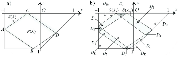
Figure 1. a). For $\lambda\in(\frac{1}{2},\frac{4}{5})$, a unique parallelogram $P(\lambda)$ can be constructed such that it is inscribed in $D$ and its sides are parallel to the straight lines of the type $x+az=C_{1}$, $x-az=C_{2}$, where $a=\sqrt{\frac{\lambda}{1-\lambda}}$.
b). For $1/2<\lambda_{*}<\lambda_{**}<4/5$, $S(\lambda_{*})$ and $S(\lambda_{**})$ divide $D$ into subdomains $D_{i}$, $i=1,2,..,13$.

These facts as well as a preliminary study of the problem by the “rays method” led the researchers to assume that there are solutions of the problem (9–11) localizing their energy in an arbitrarily small neighborhood of $S(\lambda)$ in process of time; i.e., that $S(\lambda)$ is a wave attractor (see, e.g., [23, 24, 35, 27, 28, 25, 15, 17, 36, 9, 10, 8, 13, 14, 21, 19, 26, 16, 18, 33]).

In the present paper, exact solutions to the problem (9–11) were found in an explicit form for a class of domains including trapezoid $D$. The construction of the solutions corresponds to Sobolev’s ideas of investigating of this problem and is based on the construction of piecewise constant functions which satisfy (12) and (13) in a generalized sense. The explicit form of the solutions of (9–11) makes it possible to construct some special previously unknown type of inertial waves and to investigate their properties. These waves are not inertial modes: they correspond to the continuous spectrum of inertial oscillations. Main properties of these waves are described. These waves are progressive; the main features of their energy transfer are described. The existence of these solutions casts doubt on the existence of non-point wave attractors in the tank described above.

The results of the paper were partially announced in [41].

2. Exact Solutions

Denote by $H^{1}_{0}(D)$ the subspace of the Sobolev space $H^{1}(D)$ (see, for example, [20], p. 34) consisting of functions vanishing on the boundary $\partial D$, with the inner product

(16) $$(f,g)_{1}=\int\!\!\!\int\limits_{D}\left(\nabla f,\nabla\overline{g}\right)dx\,dz.$$

On the interval $(0,+\infty)$, consider functions $\psi(x,z;\,t)$ with values in $H^{1}_{0}(D)$ such that $\psi_{t}$, $\psi_{tt}$ belong to $H^{1}_{0}(D)$ (by the derivative $\psi_{t}$, we mean the limit of $\Delta\psi/\Delta t$ as $\Delta t\to 0$ in $H^{1}_{0}(D)$–norm). Suppose $\psi_{0},\,\psi_{1}$ belong to $H^{1}_{0}(D)$. As usual, $\psi(x,z;\,t)$ is called a generalized solution to (9–11) if it satisfies (11), and for any smooth compactly supported in $D$ function $\varphi$, the equality

(17) $$\int\limits_{D}(\psi_{ttx}\varphi_{x}+\psi_{ttz}\varphi_{z}+\psi_{z}\varphi_{z})dxdz=0$$

holds for all $t>0$. It is proved in [20, 31, 34] that just these solutions are physically meaningful. If a generalized solution $\psi$ is sufficiently smooth, then it is a classical solution.

Consider the operator $\mathbf{A}_{0}:H^{1}_{0}(D)\rightarrow H^{1}_{0}(D)$ defined on smooth compactly supported in $D$ functions as the solution to the problem

(18) $$\Delta\mathbf{A}_{0}h=h_{zz},\quad\bigl{.}\mathbf{A}_{0}h\bigr{|}_{\partial D}=0,$$

and its graph closure $\mathbf{A}:H^{1}_{0}(D)\rightarrow H^{1}_{0}(D)$. It is well known that regardless of the shape of $D$ the operator $\mathbf{A}$ is a bounded self-adjoint operator and the spectrum of $\mathbf{A}$ is $[0,\,1]$ (see, e.g., [31]). Using $\mathbf{A}$ the problem (9-11) may be written in the form:

(19) $$\psi_{tt}=-\mathbf{A}\psi,\quad\psi|_{t=0}=\psi_{0},\quad\psi_{t}|_{t=0}=\psi_{1}.$$

It is easy to calculate that the equations of the sides $z=z_{i}(x,\lambda)$ of $S(\lambda)$ are:

$$CA:\quad z=1+\frac{x}{a}+\frac{1}{a}-a,\quad AB:\quad z=1-\frac{x}{a}-\frac{1}{a}-a,$$

$$BD:\quad z=\frac{x}{a}+\frac{1}{a}+a-3,\quad DC:\quad z=-\frac{x}{a}-\frac{1}{a}+a-1,$$

where $a=\sqrt{\frac{\lambda}{1-\lambda}}$, $\lambda\in(\frac{1}{2},\frac{4}{5})$ (see Figure 1a)).

Denote by $C^{1}[c,d]$ the class of functions that are continuous together with their first derivatives on an interval $[c,d]$.

Theorem 2.1.

For each $\lambda\in(\frac{1}{2},\frac{4}{5})$, define the function

(20) $$\chi(x,z,\lambda):=\left\{\begin{array}[]{ll}1,&\quad(x,z)\in P(\lambda),\\ 0,&\quad(x,z)\in D\setminus P(\lambda).\end{array}\right.$$

Then for any $\lambda_{*},\,\lambda_{**}$ satisfying the condition

(21) $$\frac{1}{2}<\lambda_{*}<\lambda_{**}<\frac{4}{5}$$

and for any $\sigma(\lambda)\in C^{1}[\frac{1}{2},\frac{4}{5}]$ , the function

(22) $$\Upsilon(x,z;\sigma;\lambda_{*},\lambda_{**}):=\int\limits_{\lambda_{*}}^{\lambda_{**}}\sigma(\mu)\chi(x,z,\mu)d\mu$$

belongs to $H_{0}^{1}(D)$.

Proof.

Define the functions $\lambda_{i}(x,y)$, $i=1,\,2,\,3,\,4$, by the formulas:

(23) $$\lambda_{1}(x,z):=\frac{(z-1)^{2}+2x^{2}+6x+4+(1-z)\sqrt{(z-1)^{2}+4(x+1)}}{2((z-1)^{2}+(x+2)^{2})},$$

(24) $$\lambda_{2}(x,z):=\frac{(z-1)^{2}+2x^{2}+2x+(1-z)\sqrt{(z-1)^{2}-4(x+1)}}{2((z-1)^{2}+x^{2})},$$

(25) $$\lambda_{3}(x,z):=\frac{(z+3)^{2}+2x^{2}+2x+(z+3)\sqrt{(z+3)^{2}-4(x+1)}}{2((z+3)^{2}+x^{2})},$$

(26) $$\lambda_{4}(x,z):=\frac{(z+1)^{2}+2x^{2}+6x+4+(1+z)\sqrt{(z+1)^{2}+4(x+1)}}{2((z+1)^{2}+(x+2)^{2})}.$$

One can verify that $z_{i}(x,\lambda_{i}(x,z))\equiv z$, $i=1,\,2,\,3,\,4$.

Under the condition (21) the parallelograms $S(\lambda_{*})$, $S(\lambda_{**})$ decompose $D$ into subdomains $D_{i}$, $i=1,2,...\,13$ (see Figure 1b)). If

$$G(\lambda):=\int_{\frac{1}{2}}^{\lambda}\sigma(\mu)\,d\mu$$

is the primitive function, then $\Upsilon(x,z;\sigma;\lambda_{*},\lambda_{**})$ coincides with the function shown at Figure 2.

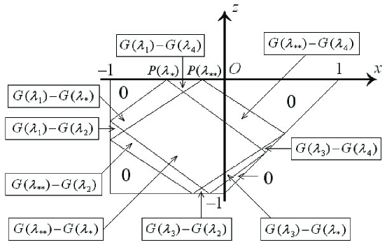
Figure 2. The piecewise presentation of the function $\Upsilon(x,z;\sigma;\lambda_{*},\lambda_{**})$.

It is easy to proof that under the condition (21) $\Upsilon(x,z;\sigma;\lambda_{*},\lambda_{**})$ is continuous and piecewise smooth in the closure $\overline{D}$. And it is obvious that $\Upsilon(x,z;\sigma;\lambda_{*},\lambda_{**})$ vanishes on the boundary $\partial D$. ∎

Unless otherwise specified, below we assume (21) to be fulfilled.

Theorem 2.2.

Suppose that in (9–11)

$${\psi}_{0}(x,z):=\int\limits_{\lambda_{*}}^{\lambda_{**}}\sigma_{0}(\lambda)\,\chi(x,z;\lambda)\,d\lambda,\quad{\psi}_{1}(x,z):=\int\limits_{\lambda_{*}}^{\lambda_{**}}\sigma_{1}(\lambda)\,\chi(x,z;\lambda)\,d\lambda,$$

where the functions $\sigma_{i}(\lambda)\in C^{1}\left[\frac{1}{2},\frac{4}{5}\right]$, $i=1,2$. Then the function

$${\psi}(x,z;t):=\!\!\int\limits_{\lambda_{*}}^{\lambda_{**}}\!\cos(\sqrt{\lambda}\;t)\,\sigma_{0}(\lambda)\,\chi(x,z;\lambda)\,d\lambda$$

(27) $$+\int\limits_{\lambda_{*}}^{\lambda_{**}}\frac{\sin(\sqrt{\lambda}\;t)}{\sqrt{\lambda}}\,\sigma_{1}(\lambda)\,\chi(x,z;\lambda)\,d\lambda,$$

is a solution to (9–11).

Proof.

For simplicity assume $\sigma_{1}\equiv 0$. For any smooth function $\varphi$ which is compactly supported in $D$, we have

$$\int\limits_{D}\!\!(\psi_{ttx}\varphi_{x}+\psi_{ttz}\varphi_{z}+\psi_{z}\varphi_{z})dxdz=\!\!\!\int\limits_{D}\!\!\left[\varphi_{x}\left(\int\limits_{\lambda_{*}}^{\lambda_{**}}\!\!\cos(\sqrt{\lambda}\;t)\,\sigma_{0}(\lambda)\,\chi(x,z;\lambda)\,d\lambda\right)_{\!\!\!ttx}\right.$$

$$+\varphi_{z}\left(\int\limits_{\lambda_{*}}^{\lambda_{**}}\cos(\sqrt{\lambda}\;t)\,\sigma_{0}(\lambda)\,\chi(x,z;\lambda)\,d\lambda\right)_{\!\!\!ttz}$$

$$+\left.\varphi_{z}\left(\int\limits_{\lambda_{*}}^{\lambda_{**}}\cos(\sqrt{\lambda}\;t)\,\sigma_{0}(\lambda)\,\chi(x,z;\lambda)\,d\lambda\right)_{\!\!\!z}\right]dxdz=$$

$$=-\int\limits_{D}\left[\varphi_{x}\left(\int\limits_{\lambda_{*}}^{\lambda_{**}}\cos(\sqrt{\lambda}\;t)\lambda\,\sigma_{0}(\lambda)\,\chi(x,z;\lambda)\,d\lambda\right)_{\!\!\!x}\right.$$

$$+\varphi_{z}\left(\int\limits_{\lambda_{*}}^{\lambda_{**}}\cos(\sqrt{\lambda}\;t)\lambda\,\sigma_{0}(\lambda)\,\chi(x,z;\lambda)\,d\lambda\right)_{\!\!\!z}$$

$$-\left.\varphi_{z}\left(\int\limits_{\lambda_{*}}^{\lambda_{**}}\cos(\sqrt{\lambda}\;t)\,\sigma_{0}(\lambda)\,\chi(x,z;\lambda)\,d\lambda\right)_{\!\!\!z}\right]dxdz=$$

$$=\int\limits_{D}\left[\varphi_{xx}\int\limits_{\lambda_{*}}^{\lambda_{**}}\cos(\sqrt{\lambda}\;t)\lambda\,\sigma_{0}(\lambda)\,\chi(x,z;\lambda)\,d\lambda\right.$$

$$+\varphi_{zz}\int\limits_{\lambda_{*}}^{\lambda_{**}}\cos(\sqrt{\lambda}\;t)\lambda\,\sigma_{0}(\lambda)\,\chi(x,z;\lambda)\,d\lambda$$

$$-\left.\varphi_{zz}\int\limits_{\lambda_{*}}^{\lambda_{**}}\cos(\sqrt{\lambda}\;t)\,\sigma_{0}(\lambda)\,\chi(x,z;\lambda)\,d\lambda\right]dxdz=$$

$$=\int\limits_{D}\left(\int\limits_{\lambda_{*}}^{\lambda_{**}}\left[\lambda\varphi_{xx}+\lambda\varphi_{zz}-\varphi_{zz}\right]\cos(\sqrt{\lambda}\;t)\,\sigma_{0}(\lambda)\,\chi(x,z;\lambda)\,d\lambda\right)dxdz=$$

$$=\int\limits_{\lambda_{*}}^{\lambda_{**}}\left(\int\limits_{D}\left[\lambda\varphi_{xx}-(1-\lambda)\varphi_{zz}\right]\cos(\sqrt{\lambda}\;t)\,\sigma_{0}(\lambda)\,\chi(x,z;\lambda)\,dxdz\right)d\lambda=$$

$$=\int\limits_{\lambda_{*}}^{\lambda_{**}}\left(\int\limits_{P(\lambda)}\left[\lambda\varphi_{xx}-(1-\lambda)\varphi_{zz}\right]\cos(\sqrt{\lambda}\;t)\,\sigma_{0}(\lambda)\,dxdz\right)d\lambda.$$

Consider the inner integral. Fix $\lambda$ and apply Green’s formula:

$$\int\limits_{P(\lambda)}\left[\lambda\varphi_{xx}-(1-\lambda)\varphi_{zz}\right]\cos(\sqrt{\lambda}\;t)\,\sigma_{0}(\lambda)\,dxdz=$$

$$=-\int\limits_{S(\lambda)}\cos(\sqrt{\lambda}\;t)\,\sigma_{0}(\lambda)\left[\lambda\varphi_{x}\cos\gamma_{1}-(1-\lambda)\varphi_{z}\cos\gamma_{2}\right]\,dS(\lambda),$$

where $S(\lambda)$ is oriented counterclockwise. We have (see Fig. 1 a):

$$\int\limits_{S(\lambda)}\cos(\sqrt{\lambda}\;t)\,\sigma_{0}(\lambda)\left[\lambda\varphi_{x}dz+(1-\lambda)\varphi_{z}dx\right]=$$

$$=\int\limits_{CA}\cos(\sqrt{\lambda}\;t)\,\sigma_{0}(\lambda)\left[\lambda\varphi_{x}dz+(1-\lambda)\varphi_{z}dx\right]+\int\limits_{AB}...+\int\limits_{BD}...+\int\limits_{DC}...$$

Consider the integral over the segment $CA$. Denote by $\widetilde{\varphi}:=\varphi|_{CA}$. As $dz=a^{-1}dx$ on the segment $CA$, it is easy to conclude that

$$\int\limits_{CA}\cos(\sqrt{\lambda}\;t)\,\sigma_{0}(\lambda)\left[\lambda\varphi_{x}dz+(1-\lambda)\varphi_{z}dx\right]=$$

$$=\int\limits_{CA}\lambda\cos(\sqrt{\lambda}\;t)\,\sigma_{0}(\lambda)\left[\varphi_{x}dz+\frac{1}{a^{2}}\,\varphi_{z}dx\right]=$$

$$=\int\limits_{C}^{A}\lambda\cos(\sqrt{\lambda}\;t)\,\sigma_{0}(\lambda)\left[\varphi_{x}\frac{1}{a}\,dx+\frac{1}{a^{2}}\,\varphi_{z}\,dx\right]=\frac{\lambda}{a}\cos(\sqrt{\lambda}\;t)\,\sigma_{0}(\lambda)\int\limits_{C}^{A}\frac{d{\widetilde{\varphi}}}{dx}dx=$$

$$=\frac{\lambda}{a}\cos(\sqrt{\lambda}\;t)\,\sigma_{0}(\lambda)\left[\widetilde{\varphi}|_{A}-\widetilde{\varphi}|_{C}\right]=0.$$

The other parts of the boundary $S(\lambda)$ can be considered similarly. So we obtain

$$\int\limits_{D}(\psi_{ttx}\varphi_{x}+\psi_{ttz}\varphi_{z}+\psi_{z}\varphi_{z})dxdz=0.$$

∎

Corollary 2.3.

Consider the primitive function

(28) $$F(\lambda,t):=\int\limits_{\lambda_{*}}^{\lambda}\left(\sigma_{0}(\mu)\cos(\sqrt{\mu}\,t)+\sigma_{1}(\mu)\frac{\sin(\sqrt{\mu}\;t)}{\sqrt{\mu}}\right)\,d\mu.$$

Then the function $\psi(x,z,t;\lambda_{*},\lambda_{**})$ defined at Figure 3 is a solution to (9–10) in $D$.

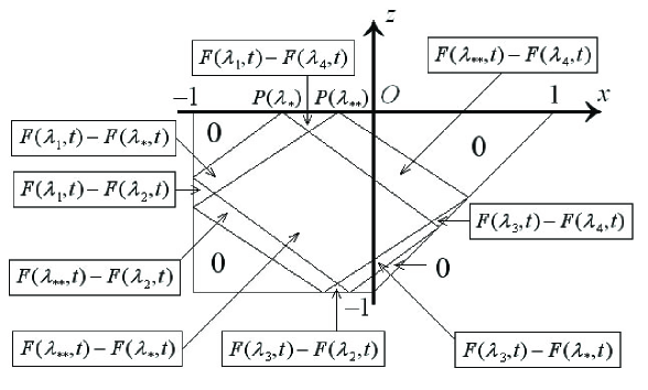
Figure 3. The piecewise presentation of $\psi(x,z,t;\lambda_{*},\lambda_{**})$.

Example 2.4.

The function $\psi(x,z,t;\lambda_{*},\lambda_{**})$ presented at Figure 4 is a solution to the problem (9–11) in $D$.

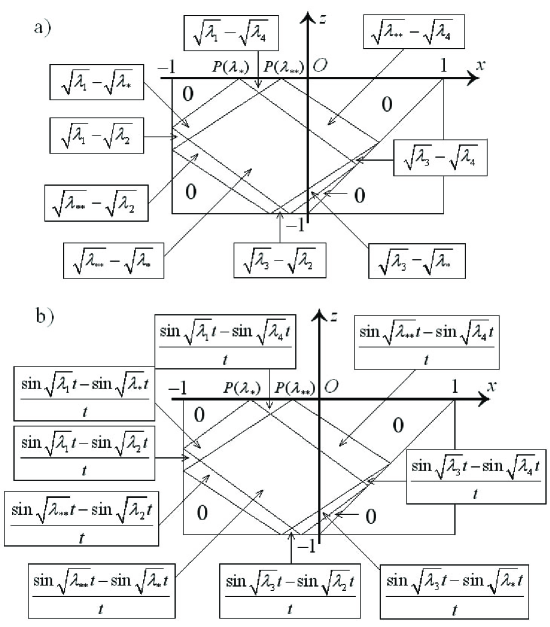
Figure 4. a) The function $\psi_{0}(x,z)$ belongs to $H_{0}^{1}(D)$. b) The solution $\psi(x,z,t;\lambda_{*},\lambda_{**})$ of (9–11) corresponding to $\psi_{0}(x,z)$ and $\psi_{1}\equiv 0$.

This follows immediately from Theorem 2.2 and Corollary 2.3 with $\sigma_{0}=\frac{1}{2\sqrt{\lambda}}$ and $\sigma_{1}\equiv 0$.

It is clear that varying $\lambda_{*}$, $\lambda_{**}$, and $\sigma_{i}$, we get inertial waves with very different properties. Choosing appropriate functions $\sigma_{i}$ it is possible to construct arbitrarily smooth solutions of this type.

Example 2.5.

If

$$F(\lambda,t)=\frac{\sin(\sqrt{\lambda}(c-t)-d)}{2(c-t)}+\frac{\sin(\sqrt{\lambda}(c+t)-d)}{2(c+t)}+\frac{\sin\sqrt{\lambda}\,t}{t}\quad\mbox{and}\,\,$$

$$F_{1}(\lambda)=\frac{\sin(c\sqrt{\lambda}-d)}{c}+\sqrt{\lambda},$$

where

$$c=\frac{2\pi}{\sqrt{\lambda}_{**}-\sqrt{\lambda}_{*}},\quad d=\frac{\pi(\sqrt{\lambda}_{**}+\sqrt{\lambda}_{*})}{\sqrt{\lambda}_{**}-\sqrt{\lambda}_{*}},$$

then the function $\psi(x,z,t;\lambda_{*},\lambda_{**})$ defined at Figure 3, is a classical solution to the problem (9 — 11) in $D$, where $\psi_{0}$ is given at Figure 5, and $\psi_{1}\equiv 0$.

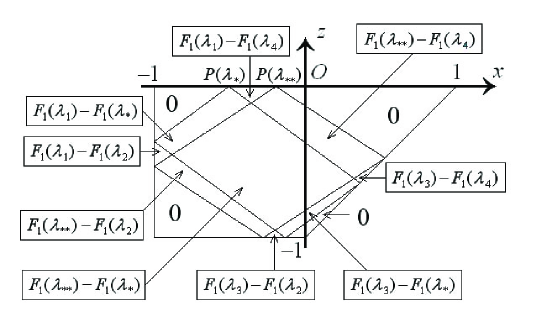
Figure 5. The initial state of the classical solution $\psi(x,z,t;\lambda_{*},\lambda_{**})$.

One can prove this by a direct calculation, but it follows from the fact that in this case $\sigma_{1}\equiv 0$ and the support of $\sigma_{0}$ lies within the interval $[\lambda_{*},\lambda_{**}]$:

(29) $$\sigma_{0}=\left\{\begin{array}[]{ll}0,&\mbox{ for }\lambda\leq\lambda_{*},\\ \frac{1}{2\sqrt{\lambda}}\left(\cos\left(\frac{2\pi\sqrt{\lambda}}{\sqrt{\lambda_{**}}-\sqrt{\lambda_{*}}}-\frac{\pi(\sqrt{\lambda_{**}}+\sqrt{\lambda_{*}})}{\sqrt{\lambda_{**}}-\sqrt{\lambda_{*}}}\right)+1\right),&\mbox{ for }\lambda_{*}<\lambda\leq\lambda_{**},\\ 0,&\mbox{ for }\lambda_{**}<\lambda.\\ \end{array}\right.$$

Now using the obtained stream function $\psi$ we can reconstruct the corresponding class of inertial waves $\mathbf{U}$ (the solutions to (5–8)). This procedure is commonly known. The components $u$ and $w$ can be found directly from the equations that determine the stream function:

$$u=-\frac{\partial{\psi}}{\partial z},\quad w=\frac{\partial{\psi}}{\partial x}.$$

According to the second equation in (5) for the component $v$ we have

(30) $$v=\int_{0}^{t}\frac{\partial\psi}{\partial z}(x,z,\tau;\lambda_{*},\lambda_{**})\,d\tau+v_{0}(x,z),$$

where $v_{0}(x,z)$ is a solution of the equation

(31) $$\frac{\partial v_{0}}{\partial z}=-\Delta\psi_{1}(x,z).$$

It is clear that (31) determines $v_{0}(x,z)$ only up to an arbitrary function $v_{*}(x)$ (of course, we are interested in the case $v\in L_{2}(D)$). The function $p(x,z,t)$ can be found from the system of equations

(32) $$\frac{\partial p}{\partial x}=\int_{0}^{t}\frac{\partial{\psi}}{\partial z}(x,z;s)\,ds+\frac{\partial}{\partial t}\frac{\partial{\psi}}{\partial z}(x,z;t)+v_{0}(x,z),$$

(33) $$\frac{\partial p}{\partial z}=-\frac{\partial}{\partial t}\frac{\partial{\psi}}{\partial x}(x,z;t).$$

Respectively $p(x,z,t)$ is determined up to the function $p_{*}(x)=\int v_{*}(x)dx$. The functions

$$\mathbf{U}_{*}=(0,v_{*}(x),0),\quad p_{*}(x)=\int v_{*}(x)dx$$

are the stationary solutions of (5–8) (see [6]).

It is obviously that the conventional characteristics (frequency, amplitude, wave vector dispersion relation, the direction of propagation of energy, and so on) can not be applied to the new found class of inertial waves.

In the next sections in order to emphasize main features of the new type of inertial waves we consider the case $\psi_{1}\equiv 0$ and $v_{0}\equiv 0$. Thus these inertial waves are $\mathbf{U}=\mathbf{U}(x,z,t;\lambda_{*},\lambda_{**})=(u,\,v,\,w)$, where

(34) $$u=-\frac{\partial{\psi}}{\partial z},\quad v=\int\limits_{0}^{t}\frac{\partial{\psi}}{\partial z}(x,z;s)\,ds,\quad w=\frac{\partial{\psi}}{\partial x},\quad u,\,v,\,w\in L_{2}(D),$$

and $\psi=\psi(x,z,t;\lambda_{*},\lambda_{**})$ corresponds to the case $\sigma_{1}\equiv 0$.

3. Geometric properties of solutions $\psi(x,z,t;\lambda_{*},\lambda_{**})$ and $\mathbf{U}(x,z,t;\lambda_{*},\lambda_{**})$

Theorem 3.1.

$\mathbf{U}(x,z,t;\lambda_{*},\lambda_{**})\equiv\mathbf{0}$ in the domains $D_{i}$, $i=9-13$ (see Figure 1b)).

Proof.

In the domains $D_{i}$, $i=10-13$ the function $\psi\equiv 0$ according to the construction. In $D_{9}$ the function $\psi$ does not depend on spatial variables, hence $\mathbf{U}(x,z,t;\lambda_{*},\lambda_{**})\equiv\mathbf{0}$ in it too. ∎

Remark 3.2.

It is easy to conclude that if $\lambda_{*}$ and $\lambda_{**}$ tend to their extreme values, i.e., $\lambda_{*}\rightarrow\frac{1}{2}$ and $\lambda_{**}\rightarrow\frac{4}{5}$, then the oscillations affect almost the entire region $D$ (see Fig. 6 a)). But if $\lambda_{*}$ and $\lambda_{**}$ are close to each other and tend to some value $\frac{1}{2}<\lambda_{***}<\frac{4}{5}$, then the region, where the oscillations take place, “tends to form the parallelogram $S(\lambda_{***})$”. The rest of the fluid is not exposed to these oscillations (see Figure 6b)).

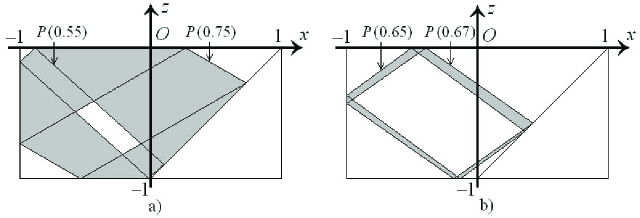
Figure 6. The comparison of areas affected by the fluid oscillations.
a) If $\lambda_{*}\rightarrow\frac{1}{2}$ and $\lambda_{**}\rightarrow\frac{4}{5}$ respectively, then the oscillations affect almost the entire domain $D$.
b) If $\lambda_{*}$ and $\lambda_{**}$ are close to each other and tend to each other, then the region, where the oscillations of the fluid take place, tends to form a parallelogram (compare with Figure 3, where the values $\lambda_{*}=0.65$ and $\lambda_{**}=0.7$ are taken).

Remark 3.3.

The construction of the solutions $\psi(x,z,t;\lambda_{*},\lambda_{**})$ and $\mathbf{U}(x,z,t;\lambda_{*},\lambda_{**})$ makes it obvious that the oscillations of this type exist not only in the trapezoid $D$, but in some rather wide class of domains. Namely, if for some fixed values $\lambda_{*}$ and $\lambda_{**}$, we arbitrarily vary the boundary $\partial D$ in those its parts which are adjacent to areas where $\psi(x,z,t)\equiv 0$, then the function $\mathbf{U}(x,z,t;\lambda_{*},\lambda_{**})$ will be a solution to (5–7) in the new domain too (see Figure 7).

This extension of the class of domains is important, because natural waters have various configurations. The geometric properties described above mean that when the oscillations of this type occur, the entire volume of the water is divided into areas of very intense oscillations and areas of complete rest. Probably, the latter phenomenon is the cause of the “strange behavior” of fish in the ocean, when a shoal is swimming in a certain direction and then turns suddenly, as if it was faced with the invisible flat wall: most likely, a zone of intense oscillations begins behind this “wall”.

Remark 3.4.

In Remark 3.3 it is shown how one can construct domains where the inertial waves of this type may occur, on the base of $D$. Of course, the trapezoid $D$ is not a distinguished domain: there are a lot of such domains. A complete description of their configurations is difficult and lays beyond the scope of this article.

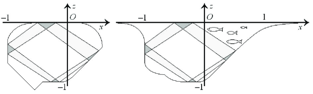
Figure 7. Some other possible configurations $D$ where this type of inertial waves can occur.

Theorem 3.5.

Suppose that $\mu_{*}<\mu_{**}$, $\mu_{*},\mu_{**}\in(\frac{1}{2},\frac{4}{5})$, $(\mu_{*},\mu_{**})\cap(\lambda_{*},\lambda_{**})=\emptyset$ and $\widetilde{\psi}(x,z,t;\mu_{*},\mu_{**})$ is a solution of the considered type (27) with some functions $\widetilde{\sigma}_{i}(\lambda)\in C^{1}\left[\frac{1}{2},\frac{4}{5}\right]$, $i=1,2$. Then the equality

$$(\psi(x,z,t;\lambda_{*},\lambda_{**}),\widetilde{\psi}(x,z,t;\mu_{*},\mu_{**}))_{1}=$$

(35) $$=\int\limits_{D}\left(\nabla\psi(x,z,t;\lambda_{*},\lambda_{**}),\nabla\overline{\widetilde{\psi}(x,z,t;\mu_{*},\mu_{**})}\right)dxdz=0$$

is true for all $t>0$.

Proof.

On the interval $(\frac{1}{2},\,\frac{4}{5})$ for an arbitrary function $\sigma(\lambda)\in C^{1}[\frac{1}{2},\,\frac{4}{5}]$, define the function $\Psi(\lambda)$ with values in $H^{1}_{0}(D)$:

(36) $$\Psi(\lambda)=\Psi(x,z;\sigma;\lambda):=\left\{\begin{array}[]{ll}\bf{0},&\mbox{ for }\lambda\leq\lambda_{*},\\ \int\limits_{\lambda_{*}}^{\lambda}\sigma(\mu)\chi(x,z;\mu)d\mu,&\mbox{ for }\lambda_{*}<\lambda\leq\lambda_{**},\\ \int\limits_{\lambda_{*}}^{\lambda_{**}}\sigma(\mu)\chi(x,z;\mu)d\mu,&\mbox{ for }\lambda_{**}<\lambda,\\ \end{array}\right.$$

where $\bf{0}$ stands for the zero element of $H^{1}_{0}(D)$. Consider the function

(37) $$\Xi:=\mathbf{A}\left(\Psi(\nu_{2})-\Psi(\nu_{1})\right)-\int\limits_{\nu_{1}}^{\nu_{2}}\lambda\,d\Psi(\lambda),$$

where the operator $\mathbf{A}$ is defined in Sec. 1, and $\nu_{1}$, $\nu_{2}$ are arbitrary in $(\frac{1}{2},\,\frac{4}{5})$. For $\lambda_{*}\leq\nu_{1}\leq\nu_{2}\leq\lambda_{**}$, we have:

$$\Xi=\mathbf{A}\,\int\limits_{\nu_{1}}^{\nu_{2}}\sigma(\lambda)\;\chi(x,z;\lambda)\,d\lambda-\int\limits_{\nu_{1}}^{\nu_{2}}\lambda\;\sigma(\lambda)\;\chi(x,z;\lambda)\,d\lambda.$$

We prove now that $\Xi=\bf{0}$. This is equivalent to prove that

$$\int\limits_{D}\left\{\frac{\partial^{2}}{\partial z^{2}}\,\int\limits_{\nu_{1}}^{\nu_{2}}\sigma(\lambda)\;\chi(x,z;\lambda)\,d\lambda\right.-\Delta\left.\int\limits_{\nu_{1}}^{\nu_{2}}\lambda\,\sigma(\lambda)\;\chi(x,z;\lambda)\,d\lambda\right\}\cdot\varphi\,dxdz=0,$$

where $\varphi$ is an arbitrary smooth function compactly supported in $D$ (the last statement means that $\Delta\Xi$ is zero element in the space $H^{-1}(D)$, see, e.g., [20]). We have:

$$\int\limits_{D}\left\{\frac{\partial^{2}}{\partial z^{2}}\,\int\limits_{\nu_{1}}^{\nu_{2}}\sigma(\lambda)\;\chi(x,z;\lambda)\,d\lambda\right.-\Delta\left.\int\limits_{\nu_{1}}^{\nu_{2}}\lambda\,\sigma(\lambda)\;\chi(x,z;\lambda)\,d\lambda\right\}\cdot\varphi\,dxdz=$$

$$=\int\limits_{D}\left\{\int\limits_{\nu_{1}}^{\nu_{2}}\sigma(\lambda)\;\chi(x,z;\lambda)\,d\lambda\cdot\frac{\partial^{2}\varphi}{\partial z^{2}}-\int\limits_{\nu_{1}}^{\nu_{2}}\lambda\;\sigma(\lambda)\;\chi(x,z;\lambda)\,d\lambda\cdot\Delta\varphi\right\}dxdz=$$

$$=\int\limits_{D}\int\limits_{\nu_{1}}^{\nu_{2}}\left\{\sigma(\lambda)\;\chi(x,z;\lambda)\cdot\frac{\partial^{2}\varphi}{\partial z^{2}}-\lambda\,\sigma(\lambda)\;\chi(x,z;\lambda)\cdot\Delta\varphi\right\}d\lambda\,dxdz=$$

$$=-\int\limits_{\nu_{1}}^{\nu_{2}}\int\limits_{D}\left\{\lambda\varphi_{xx}-(1-\lambda)\varphi_{zz}\;\right\}\chi(x,z;\lambda)\sigma(\lambda)dxdz\,d\lambda=$$

$$=-\int\limits_{\nu_{1}}^{\nu_{2}}\int\limits_{P(\lambda)}\left\{\lambda\varphi_{xx}-(1-\lambda)\varphi_{zz}\;\right\}\sigma(\lambda)dxdz\,d\lambda=0$$

(see the proof of Theorem 2.2). It is clear that $\Xi=\bf{0}$ for arbitrary $\nu_{1},\nu_{2}\in(\frac{1}{2},\,\frac{4}{5})$ too. Therefore there exist a function $h\in H^{1}_{0}(D)$ such that $\Psi(\lambda)=E_{\lambda}h$, where $E_{\lambda}$ is the resolution of the identity for $\mathbf{A}$. As for each fixed $t>0$ every solution of the type (27) can be presented in the form

$$\psi(x,z,t;\lambda_{*},\lambda_{**})=\Psi(x,z;\sigma;\,\lambda_{**})-\Psi(x,z;\sigma;\,\lambda_{*}),$$

with some appropriate $\sigma$, then the statement of the theorem follows from the condition immediately. ∎

Proposition 3.6.

Denote by $H_{c}$ the closure of the linear span of all functions of the form (36) in $H^{1}_{0}(D)$. The spectrum of the operator $\mathbf{A}$ is absolutely continuous on $H_{c}$: $\sigma(\mathbf{A}|_{H_{c}})=\sigma_{ac}(\mathbf{A}|_{H_{c}})$.

Proof.

We have to prove the absolute continuity of the function $\|\Psi(\lambda)\|_{1}^{2}$. For $\lambda_{*}\leq\lambda\leq\lambda_{**}$, we have:

$$\|\Psi(\lambda)\|_{1}^{2}=\|\Upsilon(x,z;\sigma;\lambda_{*},\lambda)\|_{1}^{2},$$

(see (22)). Denote by $D_{i}(\lambda)$ the domains corresponding to the decomposition of $D$ by $S(\lambda_{*})$ and $S(\lambda)$, $i=1,...,13$. The properties of the function $\Upsilon$ described in the proof of Theorem 2.1 allow us to assert that

$$\|\Upsilon(x,z;\sigma;\lambda_{*},\lambda)\|_{1}^{2}=\int_{D}\left|\nabla(\Upsilon(x,z;\sigma;\lambda_{*},\lambda))\right|^{2}dxdz=$$

$$=\int_{D_{1}(\lambda)}\left|\nabla(G(\lambda_{1})-G(\lambda_{4}))\right|^{2}dxdz+\int_{D_{2}(\lambda)}\left|\nabla(G(\lambda_{1})-G(\lambda_{2}))\right|^{2}dxdz$$

$$+\int_{D_{3}(\lambda)}\left|\nabla(G(\lambda_{3})-G(\lambda_{2}))\right|^{2}dxdz+\int_{D_{4}(\lambda)}\left|\nabla(G(\lambda_{3})-G(\lambda_{4}))\right|^{2}dxdz$$

$$+\sum\limits_{i=5}^{8}\int_{D_{i}(\lambda)}\left|\nabla(G(\lambda_{i-4}))\right|^{2}dxdz.$$

Here the integrands are smooth and they do not depend on $\lambda$, and all boundaries $\partial D_{i}(\lambda)$ smoothly depend on $\lambda$. Thus the function $\|\Psi(\lambda)\|_{1}^{2}$ is not only absolute continuous but smooth. ∎

The explicit form of the obtained inertial waves makes it possible to get animated graphics of the stream function, of the velocity field of the fluid, of the energy density function, etc. (See Appendix)

4. Energy properties of the solutions $\psi(x,z,t;\lambda_{*},\lambda_{**})$ and $\mathbf{U}(x,z,t;\lambda_{*},\lambda_{**})$.

All subdomains of $D$ that will be considered below are supposed to be Lipschitz domains (see definition in [20], p. 34).

Definition 4.1.

Suppose that a domain $\Omega_{0}\subset D$. If a solution of the system (5–8) is such that for any subdomain $\Omega_{1}\subset\Omega_{0}$ the amount of kinetic energy in $\Omega_{1}$

(38) $${\mathcal{E}}(t;\,\Omega_{1}):=\int\limits_{\Omega_{1}}\left(\left|u\right|^{2}+\left|v\right|^{2}+\left|w\right|^{2}\right)dxdz={\rm const}$$

(does not depend on time), then we say that the solution has the property $S$ in $\Omega_{0}$.

It is clear that each inertial mode has the property $S$ in the whole domain $D$.

Definition 4.2.

If for a solution of (5–8) in the domain $D$ there exists a subdomain $\Omega$ such that the amount of kinetic energy in $\Omega$ is not constant, then this solution is called a progressive inertial wave.

Theorem 4.3.

The solution $\mathbf{U}(x,z,t;\lambda_{*},\lambda_{**})$ has the property $S$ in the domain $\bigcup\limits_{i=5}^{13}D_{i}$.

Proof.

It is sufficient to prove that this solution has the property $S$ in the domains $D_{i}$, $i=5,...,8$. Consider, for example, the amount of kinetic energy corresponding to some domain $\Omega_{5}\subset D_{5}$:

(39) $${\mathcal{E}}(t;\,\Omega_{5})=\int_{\Omega_{5}}\left(u^{2}+v^{2}+w^{2}\right)dxdz.$$

Denote

(40) $$\Lambda:=uu_{t}+vv_{t}+ww_{t}.$$

We now show that $\Lambda\equiv 0$ in $D_{5}$. Consider the primitive function

$$F(\lambda,t):=\int_{\lambda_{*}}^{\lambda}\sigma_{0}(\mu)\cos(\sqrt{\mu}\,t)\,d\mu.$$

Then in the domain $D_{5}$

$$u=-\bigl{(}F(\lambda_{1},t)-F(\lambda_{*},t)\bigr{)}_{z}=-\frac{\partial F(\lambda_{1},t)}{\partial\lambda_{1}}\cdot\frac{\partial\lambda_{1}}{\partial z},\quad u_{t}=-\frac{\partial^{2}F(\lambda_{1},t)}{\partial t\,\partial\lambda_{1}}\cdot\frac{\partial\lambda_{1}}{\partial z},$$

$$v=\int_{0}^{t}\frac{\partial F(\lambda_{1},\tau)}{\partial\lambda_{1}}d\,\tau\cdot\frac{\partial\lambda_{1}}{\partial z},\qquad v_{t}=\frac{\partial F(\lambda_{1},t)}{\partial\lambda_{1}}\cdot\frac{\partial\lambda_{1}}{\partial z},$$

$$w=\frac{\partial F(\lambda_{1},t)}{\partial\lambda_{1}}\cdot\frac{\partial\lambda_{1}}{\partial x},\qquad w_{t}=\frac{\partial^{2}F(\lambda_{1},t)}{\partial t\,\partial\lambda_{1}}\cdot\frac{\partial\lambda_{1}}{\partial x},$$

(see (34), Theorem 2.2, and Corollary 2.3). We have

$$\frac{\partial^{2}F(\lambda_{1},t)}{\partial t\,\partial\lambda_{1}}=\bigl{(}\sigma_{0}(\lambda_{1})\cos(\sqrt{\lambda_{1}}\,t)\bigr{)}_{t}=-\sigma_{0}(\lambda_{1})\sqrt{\lambda_{1}}\sin(\sqrt{\lambda_{1}}t),$$

$$\int_{0}^{t}\frac{\partial F(\lambda_{1},\tau)}{\partial\lambda_{1}}d\,\tau=\int_{0}^{t}\sigma_{0}(\lambda_{1})\cos(\sqrt{\lambda_{1}}\,\tau)\,d\,\tau=\frac{\sigma_{0}(\lambda_{1})}{\sqrt{\lambda_{1}}}\sin(\sqrt{\lambda_{1}}t).$$

Therefore

(41) $$\Lambda=\frac{\partial F(\lambda_{1},t)}{\partial\lambda_{1}}\cdot{\sqrt{\lambda_{1}}}\sigma_{0}(\lambda_{1})\sin(\sqrt{\lambda_{1}}t)\biggl{[}\left(\frac{\partial\lambda_{1}}{\partial z}\right)^{2}\cdot\frac{1-\lambda_{1}}{\lambda_{1}}-\left(\frac{\partial\lambda_{1}}{\partial x}\right)^{2}\biggr{]}.$$

According to the definition of the function $\lambda_{1}(x,z)$

$$z_{1}(x,\lambda_{1}(x,z))\equiv z,\quad\mbox{where}\quad z_{1}(x,\lambda)=1+\frac{x}{a}+\frac{1}{a}-a,\quad a^{2}=\frac{\lambda}{1-\lambda}.$$

Denote

$$M(x,z,a):=az-x-a-1+a^{2}.$$

Using the implicit function theorem we have

$$a_{x}=-\frac{\frac{\partial M}{\partial x}}{\frac{\partial M}{\partial a}}=-\frac{-1}{z-1+2a},\quad a_{z}=-\frac{\frac{\partial M}{\partial z}}{\frac{\partial M}{\partial a}}=-\frac{a}{z-1+2a}.$$

As

$$\frac{\partial\lambda}{\partial a}=\frac{2a}{(1+a^{2})^{2}},$$

we get

$$\frac{\partial\lambda_{1}}{\partial x}=\frac{\partial\lambda_{1}}{\partial a}\frac{\partial a}{\partial x}=\left.\frac{2a}{(1+a^{2})^{2}}\cdot\frac{1}{z-1+2a}\right|_{\lambda=\lambda_{1}},$$

$$\frac{\partial\lambda_{1}}{\partial z}=\frac{\partial\lambda_{1}}{\partial a}\frac{\partial a}{\partial z}=\left.\frac{2a}{(1+a^{2})^{2}}\cdot\frac{-a}{z-1+2a}\right|_{\lambda=\lambda_{1}}.$$

Therefore, the expression in square brackets in (41) is equal to zero; respectively $\Lambda\equiv 0$ in $D_{5}$; and the amount ${\mathcal{E}}(t;\,\Omega_{5})$ of kinetic energy in $\Omega_{5}$ does not depend on time. ∎

Theorem 4.4.

(42) $${\mathcal{E}}(t;\,\bigcup\limits_{i=1}^{4}D_{i})=\sum\limits_{i=1}^{4}\int\limits_{D_{i}}\left(\left|u\right|^{2}+\left|v\right|^{2}+\left|w\right|^{2}\right)dxdz={\rm const}.$$

Proof.

The statement immediately follows from the energy conservation law (14) and Theorem 4.3. ∎

However, it is easy to establish that within the domains $D_{i}$, $i=1,2,3,4$, the amount of the kinetic energy is not constant. Thus, the inertial wave $\mathbf{U}(x,z,t;\lambda_{*},\lambda_{**})$ is progressive. It “pumps” energy from $D_{i}$ to $D_{j}$, when $i,j=1,2,3,4$, $i\neq j$, but in other areas it behaves like a standing wave.

Remark 4.5.

For all $t>0$ the energy density function is piecewise smooth in $D$ with respect to spatial variables, and there is no point in $\overline{D}$ in which it tends to infinity as $t\rightarrow\infty$.

5. Discussion: which wave attractors do exist in the trapezoid?

As it was mentioned above, papers of many authors studying inertial waves are devoted to the emergence of wave attractors. But what are wave attractors? A rigorous definition of a wave attractor does not exist until now, but from many recent papers in Geophysics and Astrophysics it becomes clear that the researchers mean that in the points of a wave attractor the energy density of a fluid tends to infinity (in some sense) as time goes to infinity.

It follows from [37] that for the considered above trapezoid $D$ (see (15)) there is no inertial mode corresponding to the frequency interval $\lambda\in(0,\frac{1}{2})$.

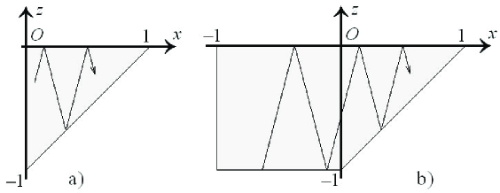
Figure 8. a) In this triangle, the vertex (1, 0) is a point wave attractor (see [38]). b) In the trapezoid $D$, the vertex (1, 0) is a possible point wave attractor.

Most likely that for the trapezoid $D$, it is possible to construct a class of inertial waves, whose energy in process of time will be concentrated in an arbitrarily small neighborhood of the vertex (1, 0) (see Figure 8b)), as it was done in the case of the triangle domain in [38]. Therefore, with a high degree of certainty, we may claim that the vertex (1, 0) is a point wave attractor (of course, this fact requires a careful mathematical proof).

Now suppose $\lambda\in(\frac{1}{2},\frac{4}{5})$. There are a lot of papers in Geophysics where the existence of wave attractors of the form $S(\lambda)$ in the trapezoid $D$ is claimed or is considered as a proven fact (see, e.g., [23, 24, 35, 27, 28, 25, 17, 36, 15, 14, 9, 10, 13, 19, 21, 26, 16, 18, 33, 8, 4]).

Alas, our opinion differs from the opinion of these authors. Namely, we are convinced that as a result of their experiments the researchers observed the oscillations of the fluid corresponding to the solutions of the described above type for some close to each other values $\lambda_{*}$ and $\lambda_{**}$ (see, for example, Figure 9). As it was shown above (Remarks 3.2, 4.5), these solutions certainly do not create attractors.

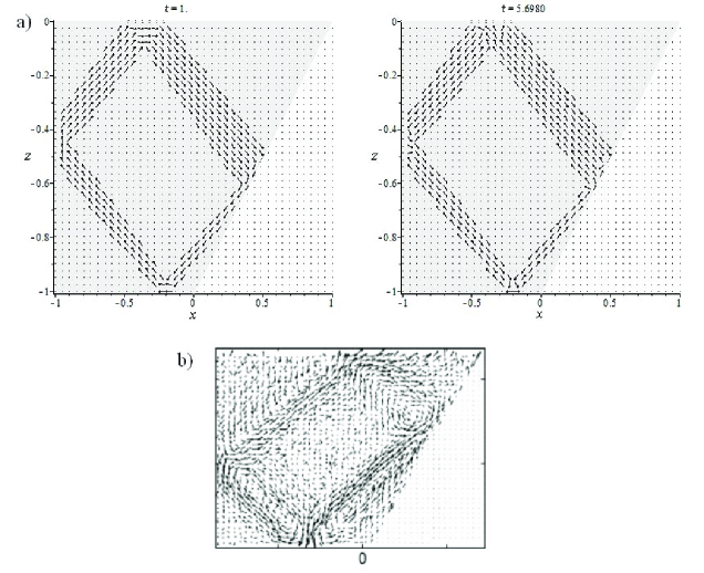
Figure 9. One can compare our field-plots of $[u,\,w]$ at different moments of time (see a)) with the velocity field in a stratified fluid in some moment (see b)) that was computed on the base of experimental measurements made by Particle Image Velocimetry in [17] (the original Figure 3a in [17]).

Of course, the question on the existence of inertial waves that can concentrate their energy in an arbitrarily small neighborhood of $S(\lambda)$ currently remains open, because to deny them one must investigate some special properties of the constructed above class of solutions, for example, their completeness in certain spaces of functions, etc., but these issues are complex and unlikely to be resolved soon.

Appendix A Some graphs

The basic properties of the obtained solutions of (5–8) were described above, but taking into account that these solutions are not almost-periodic functions, their particular properties are also very interesting and should be studied much more carefully. Here we present only a few simple graphs of these functions at certain times. We set

$$\lambda_{*}=0.65,\quad\lambda_{**}=0.7$$

and choose the function presented at the Figure 4 as the solution $\psi(x,z,t)$; the other graphs correspond to this solution too. The graphs of the function $\psi(x,z,t)$ for small values of $t$ (up to 25) and for sufficiently large $t$ (up to 2500) are presented separately. This allows to notice a substantial difference in the behavior of the function in these two cases. Although we obtained the solutions of the linearized system of equations, the study of their behavior should shed light on the formation of turbulent flows in containers having the described above configuration: as it can be seen from the graphs, the large-scale oscillations of the rotating fluid are converted to the vortex motions, the scale of which decreases when $t\to\infty$; respectively, the energy of the initial large-scale perturbation is redistributed among the micro-scale spatial fluctuations which is typical for turbulent flows.

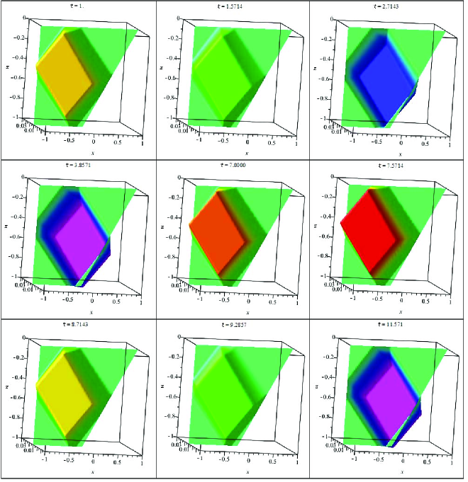
Figure 10. The unconstrained 3d-plot of the stream function $\psi(x,z,t;0.65,\,0.7)$ at some relatively small values of $t$.

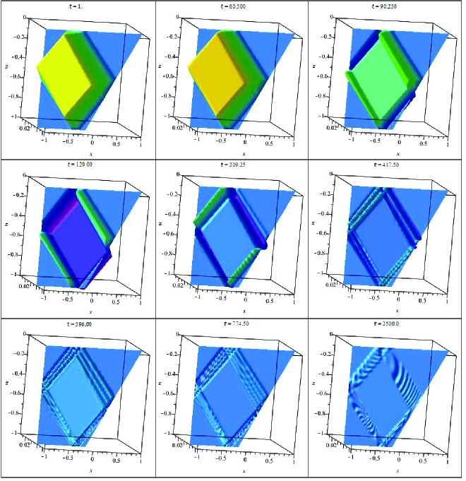
Figure 11. The unconstrained 3d-plot of the stream function $\psi(x,z,t;0.65,\,0.7)$ at some time moments.

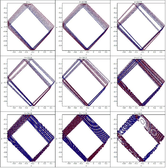
Figure 12. The contour-plot of the stream function $\psi(x,z,t;0.65,\,0.7)$ at some time moments.

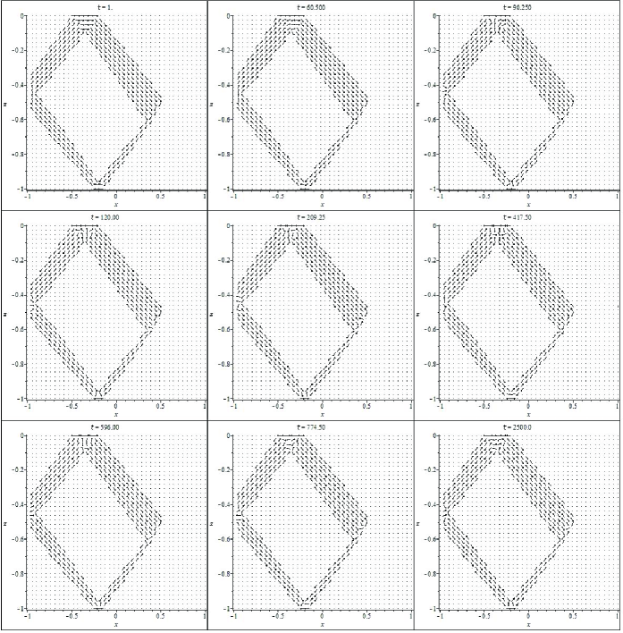
Figure 13. The field-plot $[u(x,z,t),w(x,z,t)]$ at the different values of the variable $t$.

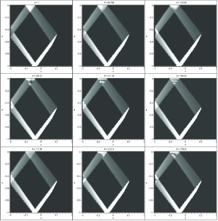
Figure 14. The plot of the energy density of the velocity field $\mathbf{U}$ at some time moments. Note, please, that this function changes as time goes on only inside 4 small triangles and in the rest of the domain $D$ it remains constant.

References

- [1] R. A. Alexandryan, On the question of the dependence of the qualitative properties of the solutions of some mixed problems on the shape of the domain, Ph.D. thesis, Moscow State University, Moscow, 1949, (In Russian).
- [2] R. A. Alexandryan, Spectral properties of operators generated by a system of differential equations of S. L. Sobolev’s type, Trudy Mosk. Mat. Obshch. 9 (1960), 455–505 (russian).
- [3] Victor Barcilon, Axi-symmetric inertial oscillations of a rotating ring of fluid, Mathematika 15 (1968), 93–102. MR 0231582 (37 #7135)
- [4] C. Brouzet, E. V. Ermanyuk, S. Joubaud, I. Sibgatullin, and T Dauxois, Energy cascade in internal-wave attractors, EPL 113 (2016), 44001.
- [5] R. T. Denchev, On the spectrum of an operator, Dokl. Akad. Nauk SSSR 126 (1959), no. 2, 259–262, (In Russian).
- [6] M. V. Fokin, Hamiltonian systems in the theory of small oscillations of a rotating ideal fluid. II, Mat. Tr. 5 (2002), no. 1, 167–204.
- [7] S. A. Gabov and A. G. Sveshnikov, Problems in the dynamics of stratified fluids, Nauka, Moscow, 1986, (In Russian).
- [8] T. Gerkema and L. Maas, Wiskundige aspecten van interne golven, Nieuw Archief voor Wiskunde 5/14 (2013), no. 3, 172–176.
- [9] T. Gerkema and J. T. F. Zimmerman, An introduction to internal waves, Royal NIOZ, 2008.
- [10] T. Gerkema, J.T.F. Zimmerman, L.R.M. Maas, and H. van Haren, Geophysical and astrophysical fluid dynamics beyond the traditional approximation, Reviews of Geophysics 46 (2008), no. 2, (RG2004).
- [11] H. P. Greenspan, The theory of rotating fluids, Cambridge University Press, 1968.
- [12] by same author, On the inviscid theory of a rotating fluids, Stud. in Appl. Math. 48 (1969), no. 1, 19–28.
- [13] Nicolas Grisouard, Chantal Staquet, and Ivane Pairaud, Numerical simulation of a two-dimensional internal wave attractor, J. Fluid Mech. 614 (2008), 1–14.
- [14] U. Harlander, Towards an analytical understanding of internal wave attractors, Adv. Geosci. 15 (2008), 3–9.
- [15] Uwe Harlander and Leo R. M. Maas, Two alternatives for solving hyperbolic boundary value problems of geophysical fluid dynamics, J. Fluid Mech. 588 (2007), 331–351.
- [16] J. Hazewinkel, C. Tsimitri, L. R. M. Maas, and S. B. Dalziel, Observations on the robustness of internal wave attractors to perturbations, Phys. Fluids 22 (2010), 107102.
- [17] J. Hazewinkel, P. van Breevoort, A. Doelman, L. R. M. Maas, and S. B. Dalziel, Equilibrium spectrum for internal wave attractor in a trapezoidal basin, Proceedings of the Fifth International Symposium on Environmental Hydraulics, Tempe, AZ (Madrid), International Association for Hydraulic Engineering and Research, 2007.
- [18] Jeroen Hazewinkel, Nicolasd Grisouard, and Stuart B. Dalziel, Comparison of laboratory and numerically observed scalar fields of an internal wave attractor, European Journal of Mechanics B/Fluids 30 (2011), 51–56.
- [19] Jeroen Hazewinkel, Pieter van Breevoort, Stuart B. Dalziel, and Leo R. M. Maas, Observations on the wavenumber spectrum and evolution of an internal wave attractor, J. Fluid Mech. 598 (2008), 373–382.
- [20] N. D. Kopachevsky and S. G. Krein, Operator approach to linear problems of hydrodynamics. Vol. 1: Self-adjoint problems for an ideal fluid, Birkhauser Verlag, Basel, Boston, Berlin, 2001.
- [21] Frans-Peter A. Lam and Leo R. M. Maas, Internal wave focusing revisited; a reanalysis and new theoretical links, Fluid Dynam. Res. 40 (2008), no. 2, 95–122.
- [22] H. Lamb, Hydrodynamics, Cambridge University Press, 1932.
- [23] L. R. M. Maas, D. Benielli, J. Sommeria, and F.-P. Lam, Observation of an internal wave attractor in a confined, stably stratified fluid, Nature 388 (1997), no. 7, 557–561.
- [24] Leo R. M. Maas, Wave focusing and ensuing mean flow due to symmetry breaking in rotating fluids, J. Fluid Mech. 437 (2001), 13–28.
- [25] by same author, Wave attractors: linear yet nonlinear, Internat. J. Bifur. Chaos Appl. Sci. Engrg. 15 (2005), no. 9, 2557–2782.
- [26] by same author, Exact analytic self-similar solution of a wave attractor field, Phys. D 238 (2009), no. 5, 502–505.
- [27] Astrid M. M. Manders and Leo R. M. Maas, Observations of inertial waves in a rectangular basin with one sloping boundary, J. Fluid Mech. 493 (2003), 59–88.
- [28] by same author, On the three-dimensional structure of the inertial wave field in a rectangular basin with one sloping boundary, Fluid Dynam. Res. 35 (2004), no. 1, 1–21.
- [29] V. P. Maslov, On the existence of a solution, decreasing as , of Sobolev’s equation for small oscillations of a rotating fluid in a cylindrical domain, Siberian Math. J. 9 (1968), no. 6, 1013–1020.
- [30] H. Poincaré, Sur l’équilibre d’une masse fluide animée d’un mouvement de rotation, Acta Math. 7 (1885), no. 1, 259–380.
- [31] J. V. Ralston, On stationary modes in inviscid rotating fluids, J. Math. Anal. Appl. 44 (1973), no. 2, 366–383.
- [32] M. Rieutord, B. Georgeot, and L. Valdettaro, Wave attractors in rotating fluids: A paradigm for ill-posed Cauchy problems, Physical Review Letters 85 (2000), no. 20, 4277–4280.
- [33] H. Scolan, E. Ermanyuk, and T Dauxois, Nonlinear fate of internal wave attractors, Phys. Rev. Lett. 110 (2013), 234501.
- [34] S. L. Sobolev, On a new problem of mathematical physics, Selected works of S. L. Sobolev, vol. I: Equations of mathematical physics, computational mathematics, and cubature formulas, Springer, New York, 2006.
- [35] C. Staquet and J. Sommeria, Internal gravity waves: from instabilities to turbulence, Annu. Rev. Fluid Mech. 34 (2002), 559–593.
- [36] Arno Swart, Gerard L. G. Sleijpen, Leo R. M. Maas, and Jan Brandts, Numerical solution of the two-dimensional Poincaré equation, J. Comput. Appl. Math. 200 (2007), no. 1, 317–341.
- [37] S. D. Troitskaya, On the first boundary value problem for a hyperbolic equation in the plane, Math. Notes 65 (1999), no. 1 2, 242–252.
- [38] by same author, Behavior as of solutions of a problem in mathematical physics, Russ. J. Math. Phys. 17 (2010), no. 3, 251–271.
- [39] by same author, The construction of exact solutions of the model problem on rotating fluid in domains with angular points, Moscow Univ. Physics Bulletin 65 (2010), no. 6, 438–445.
- [40] by same author, Solution properties of a model problem on oscillations of a rotating fluid in domains with angular points, Moscow Univ. Physics Bulletin 65 (2010), no. 6, 446–453.
- [41] by same author, An exact solution of the two-dimensional Poincaré-Sobolev equation in a trapezium, Int. Conf. “Turbulence and Wave Processes” (Moscow), INTUIT.RU, 2013, pp. 82–84.
- [42] C. Wunsch, On the propagation of the internal waves up a slope, Deep-Sea Research 15 (1968), 251–258.
- [43] by same author, Progressive internal waves on slopes, J. Fluid Mech. 35 (1969), 131–144.