An Efficient Optimal Algorithm for the Successive Minima Problem

Abstract

In many applications including integer-forcing linear multiple-input and multiple-output (MIMO) receiver design, one needs to solve a successive minima problem (SMP) on an $n$-dimensional lattice to get an optimal integer coefficient matrix $\boldsymbol{A}^{\star}\in\mathbb{Z}^{n\times n}$. In this paper, we first propose an efficient optimal SMP algorithm with an ${\mathcal{O}}(n^{2})$ memory complexity. The main idea behind the new algorithm is it first initializes with a suitable suboptimal solution, which is then updated, via a novel algorithm with only ${\mathcal{O}}(n^{2})$ flops in each updating, until $\boldsymbol{A}^{\star}$ is obtained. Different from existing algorithms which find $\boldsymbol{A}^{\star}$ column by column through using a sphere decoding search strategy $n$ times, the new algorithm uses a search strategy once only. We then rigorously prove the optimality of the proposed algorithm. Furthermore, we theoretically analyze its complexity. In particular, we not only show that the new algorithm is $\Omega(n)$ times faster than the most efficient existing algorithm with polynomial memory complexity, but also assert that it is even more efficient than the most efficient existing algorithm with exponential memory complexity. Finally, numerical simulations are presented to illustrate the optimality and efficiency of our novel SMP algorithm.

I Introduction

I-A Successive Minima Problem

Let $\boldsymbol{H}\in\mathbb{R}^{m\times n}(m\geq n)$ be an arbitrary full-column-rank matrix, then the lattice $\mathcal{L}(\boldsymbol{H})$ generated by $\boldsymbol{H}$ is defined by $\mathcal{L}(\boldsymbol{H})=\{\boldsymbol{H}\boldsymbol{a}|\boldsymbol{a}\in\mathbb{Z}^{n}\}$. For $1\leq k\leq n$, the $k$-th successive minimum $\lambda_{k}(\boldsymbol{H})$ of $\mathcal{L}(\boldsymbol{H})$ is defined as the smallest $r$ such that the closed $n$-dimensional ball $\mathbb{B}({\boldsymbol{0}},r)$ of radius $r$ centered at the origin contains $k$ linearly independent lattice vectors.

In many applications, such as integer-forcing (IF) linear multiple-input and multiple-output (MIMO) receiver design [1] [2], we need to find an invertible matrix $\boldsymbol{A}^{\star}=[\boldsymbol{a}_{1}^{\star},\boldsymbol{a}_{2}^{\star},\cdots,\boldsymbol{a}_{n}^{\star}]\in\mathbb{Z}^{n\times n}$ such that $\|\boldsymbol{H}\boldsymbol{a}_{i}^{\star}\|_{2}$ are as small as possible for $1\leq i\leq n$. By the definition of successive minima, finding such matrix $\boldsymbol{A}^{\star}$ is equivalent to solving a successive minima problem (SMP) on lattice $\mathcal{L}(\boldsymbol{H})$, which is mathematically defined in the following:

Definition 1.

SMP on lattice $\mathcal{L}(\boldsymbol{H})$: finding an invertible matrix $\boldsymbol{A}^{\star}=[\boldsymbol{a}^{\star}_{1},\ldots,\boldsymbol{a}^{\star}_{n}]\in\mathbb{Z}^{n\times n}$ such that

$$\|\boldsymbol{H}\boldsymbol{a}^{\star}_{i}\|_{2}=\lambda_{i}(\boldsymbol{H}),\quad i=1,2,\ldots,n.$$

Note that IF linear MIMO receiver reaches the optimal diversity-multiplexing tradeoff for the standard MIMO channel with no coding across transmit antennas in the high signal-to-noise ratio (SNR) region [2]. In addition to the IF linear receiver, there are many other efficient and effective MIMO detection approaches, such as the likelihood ascent search detector whose complexity is ${\mathcal{O}}(mn)$ flops [3], minimum mean-squared error iterative successive parallel arbitrated decision feedback detectors whose exact complexity analysis was not given [4], unified bit-based probabilistic data association detection approach whose complexity is substantially lower than that of the conventional symbol-based probabilistic data association detectors in uncoded V-BLAST systems using high-order QAM [5], energy spreading transform approach whose complexity is ${\mathcal{O}}(mn)$ flops [6], decision-feedback-based algorithm whose complexity is ${\mathcal{O}}(mn^{2})$ flops [7], adaptive and iterative multi-branch minimum mean-squared error decision feedback detection algorithms whose complexity is ${\mathcal{O}}(mn^{2})$ flops [8], and iterative detection and decoding algorithms for low-density parity-check codes whose exact complexity analysis was not given [9]. Different from the IF linear receiver, which decodes integer combinations of the transmitted codewords based on the fact that any integer linear combination of lattice points is still a lattice point, these detectors decode the transmitted codewords individually. When the channel matrix is near singular, the IF linear receiver may have better detection performance than these approaches.

In addition to the IF linear receiver design, solving an SMP is needed in some other applications, such as physical-layer network coding framework design [10] and compute-compress-and-forward relay strategy design [11]. Motivated by these applications, this paper focuses on developing an efficient algorithm for optimally solving the SMP and analyzing its complexity.

I-B Related works

There are several optimal SMP algorithms [12, 13, 10, 14, 15]. For conciseness, we briefly introduce the main ideas of the algorithms in the recent two papers [14, 15] only. There are two SMP algorithms in [14] which are respectively for solving SMP’s on real and complex lattices. For conciseness, we introduce the algorithm for the real SMP only. For efficiency, this algorithm first utilizes the Lenstra-Lenstra-Lovász (LLL) reduction [16] to preprocess the SMP. Then, as in [10], it finds the transformed $\boldsymbol{A}^{\star}$ column by column, by an improved Schnorr-Euchner search algorithm [17] which is a widely used sphere decoding search algorithm, in $n$ iterations. Finally, this solution is left multiplied with the unimodular matrix generated by the LLL reduction to give $\boldsymbol{A}^{\star}$. The first and last steps of the algorithm in [15] are the same as those of the algorithm in [14]. However, its second step is different. Specifically, it first creates a matrix $\boldsymbol{M}$, which stores a list of sorted (in an nondecreasing order according to their lengths) lattice vectors with lengths bounded by the largest length of all the column vectors of the LLL reduced matrix of $\boldsymbol{H}$. These vectors are obtained by employing the Alg. ALLCLOSESTPOINTS in [18]. Then $\boldsymbol{M}$ is transformed into the row echelon form by the Gaussian elimination. Finally, the first $n$ linearly independent columns of $\boldsymbol{M}$ are chosen to form the transformed $\boldsymbol{A}^{\star}$. Although simulations in this paper will show that the latter is much more efficient than the former, different from the former, its memory complexity is an exponential function in $n$. Thus, a more efficient algorithm with polynomial memory complexity is still desirable.

There are also some suboptimal SMP algorithms, such as the slowest descent method [19] and lattice reduction based algorithms [20, 21].

I-C Our Contributions

In this paper, we develop an efficient optimal SMP algorithm for $\boldsymbol{A}^{\star}$. Specifically, the contributions of this paper are summarized as follows:

• An efficient optimal algorithm for the SMP is proposed . Like existing ones, for efficiency, our algorithm first uses the LLL reduction [16] to preprocess the SMP by reducing $\boldsymbol{H}$. Then, unlike [14], which forms the solution of the transformed SMP column by column in $n$ iterations, our new algorithm initializes with a suboptimal solution which is an $n\times n$ permutation matrix such that it is a fairly good initial solution of the transformed SMP. The suboptimal solution is then updated by a novel algorithm which uses the improved Schnorr-Euchner search algorithm in [23] to search for candidates of the columns of the solution of the transformed SMP, and uses a novel and efficient algorithm to update it. The updating process continues until the optimal solution is obtained. Finally, the solution of the transformed SMP is left multiplied with the unimodular matrix generated by the LLL reduction to give the optimal solution $\boldsymbol{A}^{\star}$ (see Section II).

• We theoretically show that the memory complexity and the expected time complexity of our new algorithm are respectively ${\mathcal{O}}(n^{2})$ space and ${\mathcal{O}}(n^{3/2}(2\pi e\,m/n)^{n/2})$ flops (see Section III-A).

• We show that the new algorithm is $\Omega(n)$ times faster than the algorithm in [14], which is the most efficient existing algorithm with polynomial memory complexity (see Section III-B). We also assert that it is faster than the one in [15] whose memory complexity is exponential in $n$ (see Section III-C).

• Numerical simulations not only verify the improvements as predicted from the above theoretical findings but also show that the proposed optimal algorithm is more efficient than the Minkowski reduction based suboptimal algorithm for solving the SMP (see Section IV).

The rest of the paper is organized as follows. We propose our new SMP optimal algorithm and show its optimality in Section II. We analyze its space and time complexities in Section III. Simulation results are provided in Section IV to show the efficiency and superiority of the proposed algorithm. Finally, conclusions are given in Section V.

Notation. Let $\mathbb{R}^{m\times n}$ and $\mathbb{Z}^{m\times n}$ respectively stand for the spaces of the $m\times n$ real and integer matrices. Let $\mathbb{R}^{n}$ and $\mathbb{Z}^{n}$ denote the spaces of the $n$-dimensional real and integer column vectors, respectively. Matrices and column vectors are respectively denoted by uppercase and lowercase letters. For a matrix $\boldsymbol{A}$, let $a_{ij}$ denote its element at row $i$ and column $j$, $\boldsymbol{a}_{i}$ denote its $i$-th column, $\boldsymbol{a}_{k,i:j}$ be the vector formed by $a_{ki},a_{k,i+1},\ldots,a_{kj}$ and $\boldsymbol{A}_{i:j}$ be the submatrix of $\boldsymbol{A}$ formed by columns from $i$ to $j$. For a vector ${\boldsymbol{x}}$, let $x_{i}$ be its $i$-th element and ${\boldsymbol{x}}_{i:j}$ be the subvector of ${\boldsymbol{x}}$ formed by entries $i,i+1,\ldots,j$. For a number $x$, let $\lfloor x\rceil$ denote its nearest integer (if there is a tie, the one with smaller magnitude is chosen).

II A New SMP Algorithm

In this section, we propose an efficient algorithm for exactly solving the SMP and rigorously show its optimality.

The main novelties of our new algorithm are: one the one hand, unlike [14], which needs to use an improved Schnorr-Euchner search algorithm $n$ times, it uses the improved Schnorr-Euchner search algorithm [23] once only. On the other hand, the complexity of the novel algorithm for updating the suboptimal solution is ${\mathcal{O}}(n^{2})$ flops only. As will be explained in details in Section II-B, in comparison, a straightforward updating algorithm costs ${\mathcal{O}}(n^{4})$ flops. Because of these two novelties, the efficiency of the new algorithm is significantly improved.

II-A Preprocessing of the SMP

For efficiency, one typically uses the LLL reduction [16] to preprocess the SMP. Let $\boldsymbol{H}$ have the following thin QR factorization whose algorithms can be found in many references (see, e.g., [24]):

$$\boldsymbol{H}=\boldsymbol{Q}\boldsymbol{R},$$ (1)

where $\boldsymbol{Q}\in\mathbb{R}^{m\times n}$ is a matrix with orthonormal columns, $\boldsymbol{R}\in\mathbb{R}^{n\times n}$ is an upper triangular matrix. Recall that we assume $\boldsymbol{H}$ is a full column matrix, so $\boldsymbol{R}$ is full-rank.

After obtaining $\boldsymbol{R}$, the LLL reduction reduces $\boldsymbol{R}$ in (1) to ${\bar{\boldsymbol{R}}}$ through

$$\bar{\boldsymbol{Q}}^{T}\boldsymbol{R}\boldsymbol{Z}={\bar{\boldsymbol{R}}},$$ (2)

where $\bar{\boldsymbol{Q}}\in\mathbb{R}^{n\times n}$ is orthogonal, $\boldsymbol{Z}\in\mathbb{Z}^{n\times n}$ is unimodular (i.e., $\boldsymbol{Z}$ also satisfies $|\det(\boldsymbol{Z})|=1$), and ${\bar{\boldsymbol{R}}}\in\mathbb{R}^{n\times n}$ is an upper triangular matrix satisfying

$$|{\bar{r}}_{ik}|\leq\frac{1}{2}|{\bar{r}}_{ii}|,\quad i=1,2,\ldots,k-1,$$

$$\delta\,{\bar{r}}_{k-1,k-1}^{2}\leq{\bar{r}}_{k-1,k}^{2}+{\bar{r}}_{kk}^{2},\quad k=2,3,\ldots,n,$$

where $\delta$ is a constant satisfying $1/4<\delta\leq 1$. The matrix ${\bar{\boldsymbol{R}}}$ is said to be LLL reduced. The LLL reduction algorithm can be found in [16] and its properties in MIMO communications have been studied in [25, 26, 27].

By (1) and (2), we have $\boldsymbol{H}=\boldsymbol{Q}\bar{\boldsymbol{Q}}\bar{\boldsymbol{R}}\boldsymbol{Z}^{-1}.$ Since the columns of $\boldsymbol{Q}$ are orthonormal and $\bar{\boldsymbol{Q}}$ is orthogonal, we have

$$\|\boldsymbol{H}\boldsymbol{a}^{\star}_{i}\|_{2}=\|{\bar{\boldsymbol{R}}}\boldsymbol{Z}^{-1}\boldsymbol{a}^{\star}_{i}\|_{2},\quad 1\leq i\leq n.$$

By the definition of successive minima, we also have

$$\lambda_{i}(\boldsymbol{R})=\lambda_{i}({\bar{\boldsymbol{R}}}),\quad 1\leq i\leq n.$$

Thus, by Definition 1, the SMP on lattice $\mathcal{L}(\boldsymbol{H})$ can be transformed to the SMP on lattice $\mathcal{L}({\bar{\boldsymbol{R}}})$, i.e., Problem 1 below:

Problem 1 (SMP on lattice $\mathcal{L}({\bar{\boldsymbol{R}}})$).

finding an invertible integer matrix $\boldsymbol{B}^{\star}=[\boldsymbol{b}^{\star}_{1},\ldots,\boldsymbol{b}^{\star}_{n}]\in\mathbb{Z}^{n\times n}$ such that

$$\|{\bar{\boldsymbol{R}}}\boldsymbol{b}^{\star}_{i}\|_{2}=\lambda_{i}({\bar{\boldsymbol{R}}}),\quad 1\leq i\leq n.$$

Furthermore, if $\boldsymbol{B}^{\star}$ is a solution to Problem 1, then $\boldsymbol{A}^{\star}=\boldsymbol{Z}\boldsymbol{B}^{\star}$ is a solution to the SMP on lattice $\mathcal{L}(\boldsymbol{H})$, which is defined in Definition 1. Moreover, according to the definition of successive minima, the solution $\boldsymbol{B}^{\star}$ of Problem 1 satisfies

$$\|{\bar{\boldsymbol{R}}}\boldsymbol{b}^{\star}_{1}\|_{2}\leq\|{\bar{\boldsymbol{R}}}\boldsymbol{b}^{\star}_{2}\|_{2}\leq\cdots\leq\|{\bar{\boldsymbol{R}}}\boldsymbol{b}^{\star}_{n}\|_{2}.$$ (3)

Note that the reason for transforming the SMP on lattice $\mathcal{L}(\boldsymbol{H})$ to the SMP on lattice $\mathcal{L}({\bar{\boldsymbol{R}}})$ (i.e., Problem 1) is that the latter can be solved much more efficiently than the former due to the fact that ${\bar{\boldsymbol{R}}}$ is LLL reduced.

II-B Updating strategy for the novel algorithm

The main idea behind the proposed algorithm for Problem 1 is as follows: we start with a suboptimal solution $\boldsymbol{B}$ which is the $n\times n$ permutation matrix such that

$$\|{\bar{\boldsymbol{R}}}\boldsymbol{b}_{1}\|_{2}\leq\|{\bar{\boldsymbol{R}}}\boldsymbol{b}_{2}\|_{2}\leq\ldots\leq\|{\bar{\boldsymbol{R}}}\boldsymbol{b}_{n}\|_{2}.$$ (4)

Then, we update the suboptimal solution. More specifically, we use the improved Schnorr-Euchner search algorithm in [23] to find a nonzero integer vector $\boldsymbol{b}$ satisfying $\|{\bar{\boldsymbol{R}}}\boldsymbol{b}\|_{2}<\|{\bar{\boldsymbol{R}}}\boldsymbol{b}_{n}\|_{2}$. Then, we use it to update $\boldsymbol{B}$ and then go to the next updating. More specifically, we use $\boldsymbol{b}$ and $\boldsymbol{B}$ to get another suboptimal solution (i.e., an invertible matrix) denoting by $\bar{\boldsymbol{B}}$, whose columns are chosen from $\boldsymbol{b}$ and the columns of $\boldsymbol{B}$ such that $\|{\bar{\boldsymbol{R}}}\bar{\boldsymbol{b}}_{i}\|_{2}$ are as small as possible for $1\leq i\leq n$ and

$$\|{\bar{\boldsymbol{R}}}\bar{\boldsymbol{b}}_{1}\|_{2}\leq\|{\bar{\boldsymbol{R}}}\bar{\boldsymbol{b}}_{2}\|_{2}\leq\ldots\leq\|{\bar{\boldsymbol{R}}}\bar{\boldsymbol{b}}_{n}\|_{2}.$$ (5)

The updating process continues with the process of the improved Schnorr-Euchner enumeration until the suboptimal solution cannot be updated anymore, and the final solution is $\boldsymbol{B}^{\star}$. Note that to ensure the suboptimal solution can be updated to the optimal solution $\boldsymbol{B}^{\star}$ which satisfies (3), $\boldsymbol{B}$ should satisfy (4) and $\bar{\boldsymbol{B}}$ should satisfy (5) through the whole updating process.

From the above analysis, we can see that the updating process is equivalent to solving Problem 2 below.

Problem 2.

For a given full-rank matrix $\boldsymbol{B}\in\mathbb{Z}^{n\times n}$ and a nonzero vector $\boldsymbol{b}\in\mathbb{Z}^{n}$ which satisfy

$$r_{1}\leq r_{2}\leq\ldots\leq r_{n}\mbox{ and }\alpha<r_{n},$$ (6)

where we denote

$$r_{k}=\|{\bar{\boldsymbol{R}}}\boldsymbol{b}_{k}\|_{2},\,\;1\leq k\leq n,\mbox{ and }\alpha=\|{\bar{\boldsymbol{R}}}\boldsymbol{b}\|_{2};$$ (7)

find an invertible matrix $\bar{\boldsymbol{B}}\in\mathbb{Z}^{n\times n}$ whose column vectors are chosen from $\boldsymbol{b}$ and columns of $\boldsymbol{B}$ such that

$$\bar{r}_{1}\leq\bar{r}_{2}\leq\ldots\leq\bar{r}_{n},$$ (8)

and $\bar{r}_{i}$ are as small as possible for $1\leq i\leq n$, where we denote

$$\bar{r}_{k}=\|{\bar{\boldsymbol{R}}}\bar{\boldsymbol{b}}_{k}\|_{2},\,\;1\leq k\leq n.$$ (9)

In the following, we will propose an algorithm with at most $5n^{2}-2n-1$ flops (i.e., the summation of the numbers of addition, subtraction, multiplication and division) to solve Problem 2. In comparison, we will explain in detail that a straightforward method for Problem 2 costs ${\mathcal{O}}(n^{4})$ flops. Before giving the details, we need to show the problem is well-defined, i.e., showing the following proposition.

Proposition 1.

Problem 2 is solvable.

To prove Proposition 1, we need to introduce the following theorem:

Theorem 1.

Let $\boldsymbol{B}\in\mathbb{Z}^{n\times n}$ be an arbitrary full-rank integer matrix and $\boldsymbol{b}\in\mathbb{Z}^{n}$ be an arbitrary nonzero integer vector such that $\widetilde{\boldsymbol{B}}_{1:i}$ is full column rank for some $i$ with $1\leq i\leq n$, where

$$\widetilde{\boldsymbol{B}}=\begin{bmatrix}\boldsymbol{b}_{1}&\ldots&\boldsymbol{b}_{i-1}&\boldsymbol{b}&\boldsymbol{b}_{i}&\ldots&\boldsymbol{b}_{n}\end{bmatrix}.$$ (10)

Then there exists at least one $j$ with $i+1\leq j\leq n+1$ such that $\widetilde{\boldsymbol{B}}_{[\setminus j]}$ is also full-rank, where $\widetilde{\boldsymbol{B}}_{[\setminus j]}$ is the matrix obtained by removing the $j$-th column of $\widetilde{\boldsymbol{B}}$.

Proof.

Since $\boldsymbol{B}$ is full-rank, there exist $f_{i}\in\mathbb{R},1\leq i\leq n$, such that

$$\boldsymbol{b}=f_{1}\boldsymbol{b}_{1}+\ldots+f_{n}\boldsymbol{b}_{n}.$$

Since $\widetilde{\boldsymbol{B}}_{1:i}$ is full column rank, there exists at least one $j$ with $i+1\leq j\leq n+1$ such that $f_{j-1}\neq 0$. Otherwise, by the aforementioned equation, $\boldsymbol{b}$ is a linear combination of $\boldsymbol{b}_{1},\ldots,\boldsymbol{b}_{i-1}$ which implies that $\widetilde{\boldsymbol{B}}_{1:i}$ is not full column rank, contradicting the assumption. Then, we have

$$\begin{pmatrix}\boldsymbol{b}_{1}&\boldsymbol{b}_{2}&\ldots&\boldsymbol{b}_{j-2}&\boldsymbol{b}&\boldsymbol{b}_{j}&\ldots&\boldsymbol{b}_{n}\end{pmatrix}$$

$$= \quad\boldsymbol{B}\begin{pmatrix}1&&&f_{1}&&&\\ &\ddots&&\vdots&&&\\ &&1&f_{j-2}&&&\\ &&&f_{j-1}&&&\\ &&&f_{j}&1&&\\ &&&\vdots&&\ddots&\\ &&&f_{n}&&&1\\ \end{pmatrix}$$

which implies that

$$\begin{pmatrix}\boldsymbol{b}_{1}&\boldsymbol{b}_{2}&\ldots&\boldsymbol{b}_{j-2}&\boldsymbol{b}&\boldsymbol{b}_{j}&\ldots&\boldsymbol{b}_{n}\end{pmatrix}$$

is full-rank. Thus, $\widetilde{\boldsymbol{B}}_{[\setminus j]}$ is full-rank. ∎

Remark 1.

Note that if $i=1$, $\widetilde{\boldsymbol{B}}_{1:i}$ reduces to $\boldsymbol{b}$ which is full column rank (since $\boldsymbol{b}\neq{\boldsymbol{0}}$), and Theorem 1 reduces to:

Let $\boldsymbol{B}\in\mathbb{Z}^{n\times n}$ be an arbitrary full-rank integer matrix and $\boldsymbol{b}\in\mathbb{Z}^{n}$ be an arbitrary nonzero integer vector, then there exists at least one $j$ with $2\leq j\leq n+1$ such that the matrix obtained by removing the $j$-th column of $\begin{bmatrix}\boldsymbol{b}&\boldsymbol{b}_{1}&\ldots&\boldsymbol{b}_{n}\end{bmatrix}$ is also full-rank.

In the following, we prove Proposition 1.

Proof.

By (6) and (7), one can see that there exists an $i$ with $1\leq i\leq n$ such that $r_{i-1}\leq\alpha<r_{i}$ (note that if $i=1$, it means $\alpha<r_{1}$). Let

$$\widetilde{\boldsymbol{r}}=\begin{bmatrix}r_{1}&\ldots&r_{i-1}&\alpha&r_{i}&\ldots&r_{n}\end{bmatrix}.$$ (11)

Then, one can see that

$$\widetilde{r}_{1}\leq\widetilde{r}_{2}\leq\ldots\leq\widetilde{r}_{n+1}.$$ (12)

Hence, solving Problem 2 is equivalent to finding the largest $j$ with $1\leq j\leq n+1$ such that $\widetilde{\boldsymbol{B}}_{[\setminus j]}$ is full-rank, where $\widetilde{\boldsymbol{B}}$ is defined in (10). Specifically, after finding $j$, set $\bar{\boldsymbol{B}}=\widetilde{\boldsymbol{B}}_{[\setminus j]}$ and $\bar{\boldsymbol{r}}=\widetilde{\boldsymbol{r}}_{[\setminus j]}$, where $\widetilde{\boldsymbol{r}}_{[\setminus j]}$ is the vector obtained by removing the $j$-th entry from $\widetilde{\boldsymbol{r}}$. Then, by (7), (10) and (11), one can see that (9) holds. Moreover, by (12), one can see that $\bar{r}_{k}$ are as small as possible for $1\leq k\leq n$, and by (11) and (12), (8) holds.

If $\widetilde{\boldsymbol{B}}_{1:i}$ is not full column rank, then $j=i$, i.e., $\boldsymbol{b}$ should be removed from $\widetilde{\boldsymbol{B}}$, and the resulting matrix is $\boldsymbol{B}$ which is full-rank by assumption. This is because, no matter which $\widetilde{\boldsymbol{b}}_{j}$ is removed for $i+1\leq j\leq n+1$, the resulting matrix contains $\widetilde{\boldsymbol{B}}_{1:i}$ as a submatrix, and hence it is not full-rank. On the other hand, if $\widetilde{\boldsymbol{b}}_{j}$ is removed for $1\leq j\leq i-1$, then it is not the column with the largest index needs to be removed.

If $\widetilde{\boldsymbol{B}}_{1:i}$ is full column rank, then by Theorem 1, there exists at least one $j$ with $i+1\leq j\leq n+1$ such that $\widetilde{\boldsymbol{B}}_{[\setminus j]}$ is full-rank.

Thus, there exists a $j$ with $i\leq j\leq n+1$ such that $\widetilde{\boldsymbol{B}}_{[\setminus j]}$ is full-rank no matter whether $\widetilde{\boldsymbol{B}}_{1:i}$ is full column rank or not. Therefore, Problem 2 is solvable. ∎

By the above proof, a natural method to find the desired $j$ is to check whether $\widetilde{\boldsymbol{B}}_{[\setminus k]}$ is full-rank for $k=n+1,n,\ldots,i+1$ until finding an invertible matrix $\widetilde{\boldsymbol{B}}_{[\setminus j]}$ if it exists. Otherwise, i.e., $\widetilde{\boldsymbol{B}}_{[\setminus k]}$ is not full-rank for $k=n+1,n,\ldots,i+1$, then by the above analysis, $j=i$. Clearly, this approach works, but the main drawback of this method is that its worst complexity is ${\mathcal{O}}(n^{4})$ flops which is too high. Concretely, in the worst case, i.e., if $i=1$ and $\widetilde{\boldsymbol{B}}_{[\setminus j]}$ are not full-rank for $2\leq j\leq n+1$, then $n$ matrices need to be checked. Since the complexity of checking whether an $n\times n$ matrix is full-rank or not is ${\mathcal{O}}(n^{3})$ flops, the whole complexity is ${\mathcal{O}}(n^{4})$ flops.

In the following, we propose a method which solves Problem 2 in ${\mathcal{O}}(n^{2})$ flops, under the assumption that $\boldsymbol{B}$ has the LU factorization $\boldsymbol{L}\boldsymbol{B}=\boldsymbol{U}$ with given $\boldsymbol{L}$ and $\boldsymbol{U}$, by using an updating LU factorization algorithm. Specifically, we have the following theorem:

Theorem 2.

Let $\boldsymbol{B}$ be defined in Problem 2, suppose that $\boldsymbol{B}$ has the following LU factorization:

$$\boldsymbol{L}\boldsymbol{B}=\boldsymbol{U},$$ (13)

where full-rank matrix $\boldsymbol{L}\in\mathbb{R}^{n\times n}$ is a product of lower triangular and permutation matrices and $\boldsymbol{U}\in\mathbb{R}^{n\times n}$ is an invertible upper triangular matrix. Then there exists an algorithm with at most $5n^{2}-2n-1$ flops to find $\bar{\boldsymbol{B}}$ and $\bar{\boldsymbol{r}}$ which satisfy the requirement of Problem 2, and full-rank matrices $\bar{\boldsymbol{L}}\in\mathbb{R}^{n\times n}$ and $\bar{\boldsymbol{U}}\in\mathbb{R}^{n\times n}$, which are respectively a product of lower triangular and permutation matrices and upper triangular matrix, such that

$$\bar{\boldsymbol{L}}\bar{\boldsymbol{B}}=\bar{\boldsymbol{U}}.$$ (14)

Before proving Theorem 2, we make a comment.

Remark 2.

Theorem 2 shows that Problem 2 can be solved by an algorithm with at most $5n^{2}-2n-1$ flops under the condition that the LU factorization of $\boldsymbol{B}$ (see (13)) is given (note that the LU factorization of $\boldsymbol{B}$ is usually expressed as $\boldsymbol{B}=\boldsymbol{L}\boldsymbol{U}$, but as can be seen from the following proof, it is better to use $\boldsymbol{L}\boldsymbol{B}=\boldsymbol{U}$). Recall that the initial $\boldsymbol{B}$ of our new algorithm for Problem 1 is a permutation matrix, (see the first paragraph of this subsection), so (13) holds by setting $\boldsymbol{L}=\boldsymbol{B}$ and $\boldsymbol{U}=\boldsymbol{I}$. Furthermore, Theorem 2 shows that, in addition to returning $\bar{\boldsymbol{B}}$ and $\bar{\boldsymbol{r}}$ as required in Problem 2, the algorithm also returns $\bar{\boldsymbol{L}}$ and $\bar{\boldsymbol{U}}$ such that (14) holds, thus assuming that we have the LU factorization of $\boldsymbol{B}$ is not a problem.

Proof.

In the following, we propose an algorithm to find $\bar{\boldsymbol{B}}$, $\bar{\boldsymbol{r}}$, $\bar{\boldsymbol{L}}$ and $\bar{\boldsymbol{U}}$ satisfying the requirement of Theorem 2, and then show its complexity is at most $5n^{2}-2n-1$ flops.

Our method for Problem 2 consists of three steps. Firstly, we find $i$ with $r_{i-1}\leq\alpha<r_{i}$ such that (11) and (12) hold to form $\widetilde{\boldsymbol{B}}$ (see (10)). Then, we find the largest $j$ such that $\widetilde{\boldsymbol{B}}_{[\setminus j]}$ is full-rank. Finally, we get $\bar{\boldsymbol{B}}$ by setting $\bar{\boldsymbol{B}}=\widetilde{\boldsymbol{B}}_{[\setminus j]}$, obtain $\bar{\boldsymbol{r}}$ by setting $\bar{\boldsymbol{r}}=\widetilde{\boldsymbol{r}}_{[\setminus j]}$ and update $\boldsymbol{L}$ and $\boldsymbol{U}$ to $\bar{\boldsymbol{L}}$ and $\bar{\boldsymbol{U}}$, respectively.

The first step is trivial, so in the following, we consider the second step. By (13), we have

$$\boldsymbol{L}\begin{bmatrix}\boldsymbol{B}&\boldsymbol{b}\end{bmatrix}=\begin{bmatrix}\boldsymbol{U}&\boldsymbol{L}\boldsymbol{b}\end{bmatrix}:=\tilde{\boldsymbol{U}},$$ (15)

where we denote $\tilde{\boldsymbol{U}}=\begin{bmatrix}\boldsymbol{U}&\boldsymbol{L}\boldsymbol{b}\end{bmatrix}\in\mathbb{R}^{n\times(n+1)}$. Since $\boldsymbol{L}$ is an invertible matrix and $j\geq i$ (see the proof of Proposition 1), finding the desired $j$ is equivalent to finding the largest $j$ with $i\leq j\leq n$ such that $\widetilde{\boldsymbol{U}}_{[\setminus j]}$ is full-rank if it exists. Specifically, by the proof of Proposition 1, if there exist $i\leq j\leq n$ such that $\widetilde{\boldsymbol{U}}_{[\setminus j]}$ is full-rank, then the largest $j$ is the one we need; otherwise, the last column of $\begin{bmatrix}\boldsymbol{B}&\boldsymbol{b}\end{bmatrix}$ should be removed to form $\bar{\boldsymbol{B}}$. Since $\tilde{\boldsymbol{U}}_{1:n}$ is an upper triangular matrix, by (15), to find the desired $j$, we only need to check whether $\tilde{u}_{k,n+1}\neq 0$ for $k=n,n-1,\ldots,i$ until finding one $j$ such that $\tilde{u}_{j,n+1}\neq 0$ if it exists. Otherwise, i.e., $\tilde{u}_{k,n+1}=0$ for $k=n,n-1,\ldots,i$, then we set $\bar{\boldsymbol{B}}=\boldsymbol{B}$, $\bar{\boldsymbol{r}}=\boldsymbol{r}$, $\bar{\boldsymbol{L}}=\boldsymbol{L}$ and $\bar{\boldsymbol{U}}=\boldsymbol{U}$.

In the following, we introduce the last step. If $\tilde{u}_{k,n+1}=0$ for $k=n,n-1,\ldots,i$, then by the above analysis, $\bar{\boldsymbol{B}}=\boldsymbol{B}$, $\bar{\boldsymbol{r}}=\boldsymbol{r}$, $\bar{\boldsymbol{L}}=\boldsymbol{L}$ and $\bar{\boldsymbol{U}}=\boldsymbol{U}$. Otherwise, there exist at least one $i<j\leq n$ such that $\tilde{u}_{j,n+1}\neq 0$. Then we set $\bar{\boldsymbol{B}}=\widetilde{\boldsymbol{B}}_{[\setminus j]}$ and $\bar{\boldsymbol{r}}=\widetilde{\boldsymbol{r}}_{[\setminus j]}$. To get $\bar{\boldsymbol{L}}$, $\bar{\boldsymbol{U}}$, we first update $\tilde{\boldsymbol{U}}$ to $\hat{\boldsymbol{U}}$ by setting

$$\hat{\boldsymbol{U}}=\begin{bmatrix}\boldsymbol{U}_{1:i-1}&\boldsymbol{L}\boldsymbol{b}&\boldsymbol{U}_{i:j-1}&\boldsymbol{U}_{j+1:n}\end{bmatrix}.$$

Then, we use elementary transformations of matrices to bring $\hat{\boldsymbol{U}}$ back to an upper triangular matrix by transforming $\hat{u}_{ki}=0$ for $k=j,\ldots,i+1$ to get $\bar{\boldsymbol{U}}$. Meanwhile, we use the same elementary transformations to update $\boldsymbol{L}$ to get $\bar{\boldsymbol{L}}$.

To make readers implement the above algorithm easily, we describe the pseudocode of the above algorithm in Alg. 1.

Algorithm 1 An efficient updating LU factorization algorithm for updating $\boldsymbol{B}$

Input: An invertible matrix $\boldsymbol{B}\in\mathbb{Z}^{n\times n}$, nonzero vectors $\boldsymbol{r}\in\mathbb{R}^{n}$ and $\boldsymbol{b}\in\mathbb{Z}^{n}$, and positive number $\alpha$ that satisfy (6) and (7), an invertible upper triangular $\boldsymbol{U}$ and full-rank matrix $\boldsymbol{L}$ such that (13) holds.

Output: An invertible matrix $\bar{\boldsymbol{B}}$ and a nonzero vector $\bar{\boldsymbol{r}}$ satisfy the requirement of Problem 2, an invertible upper triangular matrix $\bar{\boldsymbol{U}}$ and an invertible matrix $\bar{\boldsymbol{L}}$ such that (14) holds.

1:  set $n=$length$(\boldsymbol{b})$;

2:  $\boldsymbol{v}=\boldsymbol{L}\boldsymbol{b}$;  // use $\boldsymbol{v}$ to store $\boldsymbol{L}\boldsymbol{b}$ (see (15))

3:  find $i$ such that $r_{i-1}\leq\alpha<r_{i}$;

4:  find $j$ which is the largest $k$ such that $v_{k}\neq 0$;

5:  if $j<i$ then

6:     set $\bar{\boldsymbol{B}}=\boldsymbol{B}$, $\bar{\boldsymbol{r}}=\boldsymbol{r}$, $\bar{\boldsymbol{L}}=\boldsymbol{L},\bar{\boldsymbol{U}}=\boldsymbol{U}$;

7:  else

8:     set $\bar{\boldsymbol{L}}=\boldsymbol{L}$;

9:     set $\bar{\boldsymbol{U}}=\begin{bmatrix}\boldsymbol{U}_{1:i-1}&\boldsymbol{v}&\boldsymbol{U}_{i:j-1}&\boldsymbol{U}_{j+1:n}\end{bmatrix}$ // we denote $\boldsymbol{v}=\boldsymbol{L}\boldsymbol{b}$ (see line 2)

10:     set $\bar{\boldsymbol{B}}=\begin{bmatrix}\boldsymbol{B}_{1:i-1}&\boldsymbol{b}&\boldsymbol{B}_{i:j-1}&\boldsymbol{B}_{j+1:n}\end{bmatrix}$

11:     set $\bar{\boldsymbol{r}}=\begin{bmatrix}\boldsymbol{r}_{1:i-1}&\alpha&\boldsymbol{r}_{i:j-1}&\boldsymbol{r}_{j+1:n}\end{bmatrix}$

12:     if $j>i$ then

13:        for $k=j:-1:i+1$ do

14:           if $\bar{u}_{k-1,i}=0$ then

15:              swap the $(k-1)$-th and $k$-th rows of $\bar{\boldsymbol{U}}$, and $(k-1)$-th and $k$-th rows of $\bar{\boldsymbol{L}}$

16:           else

17:              set $t=\bar{u}_{ki}/\bar{u}_{k-1,i}$, $\bar{u}_{ki}=0$;

18:              $\bar{\boldsymbol{u}}_{k,k:n}=\bar{\boldsymbol{u}}_{k,k:n}-t\bar{\boldsymbol{u}}_{k-1,k:n}$;

19:              $\bar{\boldsymbol{l}}_{k,1:n}=\bar{\boldsymbol{l}}_{k,1:n}-t\bar{\boldsymbol{l}}_{k-1,1:n}$;

20:           end if

21:        end for

22:     end if

23:  end if

In the following, we analyze the complexity of Alg. 1 by counting the number of flops. Since $\boldsymbol{L}$ may not be a lower triangular matrix, the first 11 steps cost at most $2n^{2}$ flops (for computing $\boldsymbol{v}$), and the last 12 steps cost

$$2\sum^{j}_{k=i+1}(2n-k+1.5)\leq 2\sum^{n}_{k=2}(2n-k+1.5)=3n^{2}-2n-1$$

flops. Thus, the total complexity of Alg. 1 is at most $5n^{2}-2n-1$ flops. From the above analysis, we can see that, if $i$ is large or $j$ is small, the total complexity of Alg. 1 is much smaller than $5n^{2}-2n-1$ flops. ∎

Example 1.

Let

$${\bar{\boldsymbol{R}}}=\begin{bmatrix}2&0&0&0\\ 0&2&1&0\\ 0&0&2&0\\ 0&0&0&2\end{bmatrix},\,\;\boldsymbol{B}=\begin{bmatrix}1&0&0&0\\ 0&2&0&0\\ 0&0&3&0\\ 0&0&0&4\end{bmatrix},\,\;\boldsymbol{b}=\begin{bmatrix}1\\ -1\\ 1\\ 0\end{bmatrix},$$ (16)

$\boldsymbol{r}=\begin{bmatrix}2&4&3\sqrt{5}&8\end{bmatrix}^{T}$ and $\alpha=3$. Then, (6) and (7) hold. In the following, we show how to obtain $\bar{\boldsymbol{B}}$, $\bar{\boldsymbol{r}}$, $\bar{\boldsymbol{L}}$ and $\bar{\boldsymbol{U}}$ such that $\bar{\boldsymbol{L}}\bar{\boldsymbol{B}}=\bar{\boldsymbol{U}}$.

By (16), one can easily obtain that

$$\boldsymbol{L}=\begin{bmatrix}1&0&0&0\\ 0&1&0&0\\ 0&0&1&0\\ 0&0&0&1\end{bmatrix},\,\;\boldsymbol{U}=\begin{bmatrix}1&0&0&0\\ 0&2&0&0\\ 0&0&3&0\\ 0&0&0&4\end{bmatrix}$$

such that (13) holds. Since $\boldsymbol{r}=\begin{bmatrix}2&4&3\sqrt{5}&8\end{bmatrix}^{T}$ and $\alpha=3$, by line 3 of Alg. 1, $i=2$. By line 2 of Alg. 1 $\boldsymbol{v}=\begin{bmatrix}1&-1&1&0\end{bmatrix}^{T}$, thus $j=3>i$ (see line 4 of Alg. 1)). Then, by lines 9-11 of Alg. 1, we obtain

$$\bar{\boldsymbol{U}}=\begin{bmatrix}1&1&0&0\\ 0&-1&2&0\\ 0&1&0&0\\ 0&0&0&4\end{bmatrix},\,\;\bar{\boldsymbol{B}}=\begin{bmatrix}1&1&0&0\\ 0&-1&2&0\\ 0&1&0&0\\ 0&0&0&4\end{bmatrix},\,\;\bar{\boldsymbol{r}}=\begin{bmatrix}2\\ 3\\ 4\\ 8\end{bmatrix}.$$

Since $j=3>2=i$, by lines 13-21 of Alg. 1, we get

$$\bar{\boldsymbol{L}}=\begin{bmatrix}1&0&0&0\\ 0&1&0&0\\ 0&1&1&0\\ 0&0&0&1\end{bmatrix},\,\;\bar{\boldsymbol{U}}=\begin{bmatrix}1&1&0&0\\ 0&-1&2&0\\ 0&0&2&0\\ 0&0&0&4\end{bmatrix}.$$

It is easy to check that $\bar{\boldsymbol{B}}$ and $\bar{\boldsymbol{r}}$ satisfy (8) and (9), and $\bar{\boldsymbol{L}}\bar{\boldsymbol{B}}=\bar{\boldsymbol{U}}$.

II-C The improved Schnorr-Euchner search algorithm in [23]

From the first paragraph of Sec. II-B, our novel algorithm for Problem 1 needs to use the integer vectors obtained by the improved Schnorr-Euchner search algorithm [23] to update the suboptimal solution $\boldsymbol{B}$, thus we briefly review this algorithm in this subsection. To better explain this algorithm, we first introduce the Schnorr-Euchner search algorithm [28] for solving the following shortest vector problem (SVP)

$$\boldsymbol{b}^{\star}=\min_{\boldsymbol{b}\in\mathbb{Z}^{n}\backslash\{0\}}\|{\bar{\boldsymbol{R}}}\boldsymbol{b}\|_{2}.$$ (17)

More details on this algorithm are referred to [18, 29], and its variants can be found in [30, 31].

Suppose that $\boldsymbol{b}^{\star}$ is within the hyper-ellipsoid defined by

$$\left\lVert\bar{\boldsymbol{R}}\boldsymbol{b}\right\rVert_{2}<\beta,$$ (18)

where $\beta$ is a given constant. Let

$$d_{n}=0,\;d_{i}=-\frac{1}{\bar{r}_{ii}}\sum_{j=i+1}^{n}\bar{r}_{ij}b_{j},\quad i=n-1,\ldots,1.$$ (19)

Then (18) can be transformed to

$$\sum_{i=1}^{n}\bar{r}_{ii}^{2}(b_{i}-d_{i})^{2}<\beta^{2}$$

which is equivalent to

$$\bar{r}_{ii}^{2}(b_{i}-d_{i})^{2}<\beta^{2}-\sum_{j=i+1}^{n}\bar{r}_{jj}^{2}(b_{j}-d_{j})^{2}$$ (20)

for $i=n,n-1,\ldots,1$, where $i$ is called as the level index, and we define $\sum_{j=n+1}^{n}\bar{r}_{jj}^{2}(b_{j}-d_{j})^{2}:=0$.

The Schnorr-Euchner search algorithm starts with $\beta=\infty$, and sets $b_{i}=\lfloor d_{i}\rceil$ ($d_{i}$ are computed via (19)) for $i=n,n-1,\ldots,1$. Clearly, $\boldsymbol{b}={\boldsymbol{0}}$ is obtained and (20) holds. Since $\boldsymbol{b}^{\star}\neq{\boldsymbol{0}}$, $\boldsymbol{b}$ should be updated. To be more specific, $b_{1}$ is set as the next closest integer to $d_{1}$. Since $\beta=\infty$, (20) with $i=1$ holds. Thus, this updated $\boldsymbol{b}$ is stored and $\beta$ is updated to $\beta=\left\lVert\boldsymbol{R}\boldsymbol{b}\right\rVert_{2}$. Then, the algorithm tries to update the latest found $\boldsymbol{b}$ by finding a new $\boldsymbol{b}$ satisfying (18). Since (20) with $i=1$ is an equality for the current $\boldsymbol{b}$, $b_{1}$ only cannot be updated. Thus we try to update $b_{2}$ by setting it as the next closest integer to $d_{2}$. If it satisfies (20) with $i=2$, we try to update $b_{1}$ by setting $b_{1}=\lfloor d_{1}\rceil$ and then check whether (20) with $i=1$ holds or not, and so on; Otherwise, we try to update $b_{3}$, and so on. Finally, when we are not able to find a new integer $\boldsymbol{b}$ such that (20) holds with $i=n$, the search process stops and outputs the latest $\boldsymbol{b}$, which is actually $\boldsymbol{b}^{\star}$ satisfying (17).

The improved Schnorr-Euchner search algorithm [23] is a simple modification of the Schnorr-Euchner search algorithm based on the fact that if $\boldsymbol{b}^{\star}$ is an optimal solution to (17), then so is $-\boldsymbol{b}^{\star}$. Specifically, the algorithm in [23] only searches the nonzero integer vectors $\boldsymbol{b}$, satisfying $b_{n}\geq 0$ and $b_{i}\geq 0$ if $\boldsymbol{b}_{i+1:n}={\boldsymbol{0}}$ ($1\leq i\leq n-1$). Note that only the former property of $\boldsymbol{b}$ is exploited in [14], whereas this strategy can prune more vectors while retaining optimality.

II-D A novel optimal SMP algorithm

In this subsection, we develop a novel and efficient algorithm for SMP on lattice $\mathcal{L}(\boldsymbol{H})$. We begin with designing the algorithm for Problem 1 by incorporating Alg. 1 into the Schnorr-Euchner search algorithm.

The proposed algorithm for Problem 1 is described as follows: we start with a suboptimal solution $\boldsymbol{B}$ which is the $n\times n$ permutation matrix satisfying (4) and assume $\beta=\|{\bar{\boldsymbol{R}}}\boldsymbol{b}_{n}\|_{2}$. We further assume $\boldsymbol{L}=\boldsymbol{B}$, $\boldsymbol{U}$ is the $n\times n$ identity matrix, $\boldsymbol{r}\in\mathbb{R}^{n}$ with $r_{k}=\|{\bar{\boldsymbol{R}}}\boldsymbol{b}_{k}\|_{2}$ for $1\leq k\leq n$. Clearly, $\boldsymbol{r}$ satisfies (6) and (7), and (13) holds (note that $\boldsymbol{B}$ is a permutation matrix). Then we use the improved Schnorr-Euchner search algorithm [23] to search nonzero integer vectors $\boldsymbol{b}$ satisfying (18) to update $\boldsymbol{B}$. Specifically, we denote $\alpha=\|{\bar{\boldsymbol{R}}}\boldsymbol{b}\|_{2}$ (since $\boldsymbol{b}$ satisfies (18) and $\beta=\|{\bar{\boldsymbol{R}}}\boldsymbol{b}_{n}\|$, $\alpha$ satisfies (6)), use Alg. 1 to update $\boldsymbol{B}$, $\boldsymbol{r}$, $\boldsymbol{L}$ and $\boldsymbol{U}$ and set $\beta=r_{n}$. After this, we go to the next updating, i.e., we use the improved Schnorr-Euchner search algorithm to update $\boldsymbol{b}$ and $\alpha$ (more details on how to update $\boldsymbol{b}$ is referred to Sec. II-C), and then use Alg. 1 to update $\boldsymbol{B}$, $\boldsymbol{r}$, $\boldsymbol{L}$ and $\boldsymbol{U}$. Finally, when $\boldsymbol{B}$ cannot be updated anymore and $\beta$ cannot be decreased anymore (i.e., when we are not able to find a new value for $b_{n}$ such that (20) holds with $k=n$), the search process stops and outputs $\boldsymbol{B}^{\star}$.

By the above analysis, the proposed algorithm for Problem 1 can be summarized in Alg. 2, where

$$\mbox{sgn}(x)=\begin{cases}1,&x\geq 0\cr-1,&x<0\end{cases}.$$ (21)

Algorithm 2 A sphere decoding based algorithm for Problem 1

Input: A nonsingular upper triangular ${\bar{\boldsymbol{R}}}\in\mathbb{R}^{n\times n}$.

Output: A solution $\boldsymbol{B}^{\star}$ to Problem 1.

1:  $n=$length$(u)$;

2:  $\boldsymbol{b}={\boldsymbol{0}}$;

3:  $\boldsymbol{d}={\boldsymbol{0}}$ ($n\times 1$ zero vector); // see (19)

4:  $\boldsymbol{r}={\boldsymbol{0}}$;

5:  for i=1:n do

6:     $r_{i}=\|\bar{\boldsymbol{r}}_{i}\|_{2}$; // $r_{i}=\|{\bar{\boldsymbol{R}}}\boldsymbol{b}_{i}\|_{2}$;

7:  end for

8:  $[\boldsymbol{r},\mbox{order}]=\mbox{sort}(\boldsymbol{r})$, $\beta=r_{n}$; //initial radius, see (18)

9:  $\boldsymbol{B}=\boldsymbol{I}_{n}$, $\boldsymbol{B}=\boldsymbol{B}(:,\mbox{order})$; //initial $\boldsymbol{B}$ which is a permutation matrix and satisfies (4),

10:  $\bar{\boldsymbol{L}}=\boldsymbol{B},\boldsymbol{U}=\boldsymbol{I}_{n}$ // $\bar{\boldsymbol{L}},\boldsymbol{U}$ satisfy $\bar{\boldsymbol{L}}\boldsymbol{B}=\boldsymbol{I}_{n}$;

11:  $\boldsymbol{\xi}={\boldsymbol{0}}$; // $\xi_{i}=\sum_{j=i+1}^{n}\bar{r}_{jj}^{2}(b_{j}-d_{j})^{2}$ (see (20))

12:  $\boldsymbol{s}={\boldsymbol{0}}$; // used to update the entries of $\boldsymbol{b}$

13:  $i=n$;

14:  $\gamma=0$;

15:  while 1 do

16:     $\eta=\xi_{i}+\gamma^{2}$;

17:     if $\eta<\beta^{2}$ then

18:        if $k\neq 1$ then

19:           $i=i-1$;

20:           $\xi_{i}=\eta$;

21:           $d_{i}=-\frac{1}{\bar{r}_{ii}}\sum_{j=i+1}^{n}\bar{r}_{ij}b_{j}$; // see (19)

22:           $b_{i}=\lfloor d_{i}\rceil$;

23:           $\gamma=\bar{r}_{ii}(d_{i}-b_{i})$;

24:           $s_{i}=\mbox{sgn}(d_{i}-b_{i})$; //(see (21))

25:        else

26:           if $\eta\neq 0$ then

27:              use Alg. 1 to update $\bar{\boldsymbol{L}}$, $\boldsymbol{U}$, $\boldsymbol{B}$ and $\boldsymbol{r}$, where $\alpha=\sqrt{\eta}$, set $\beta=r_{n}$;

28:              set $i=i+1$;

29:           end if

30:           $b_{i}=b_{i}+s_{i}$;

31:           $\gamma=\bar{r}_{ii}(d_{i}-b_{i})$;

32:           $s_{i}=-s_{i}-$sgn$(s_{i})$;

33:        end if

34:     else

35:        if $i=n$ then

36:           break;

37:        else

38:           $i=i+1$;

39:           if $i=n$ then

40:              $b_{i}=b_{i}+1$;

41:           else

42:              if $\boldsymbol{b}_{i+1:n}={\boldsymbol{0}}$ then

43:                 $b_{i}=b_{i}+1$ 

44:              else

45:                 $b_{i}=b_{i}+s_{i}$;

46:                 $s_{i}=-s_{i}-$sgn$(s_{i})$;

47:              end if

48:           end if

49:           $\gamma=\bar{r}_{ii}(d_{i}-b_{i})$;

50:        end if

51:     end if

52:  end while

Remark 3.

Note that the differences between Alg. 2 and the improved Schnorr-Euchner search algorithm in [23] are lines 4-10 and line 27 which are for initialization and updating suboptimal solutions $\boldsymbol{B}$, respectively. More specifically, lines 4-10 and line 27 should be respectively changed to $\bar{\boldsymbol{b}}={\boldsymbol{0}}$ (intermediate solution), and $\bar{\boldsymbol{b}}=\boldsymbol{b},\beta=\eta$ for the improved Schnorr-Euchner search algorithm.

If $\boldsymbol{B}^{\star}$ is a solution to Problem 1, then $\boldsymbol{A}^{\star}=\boldsymbol{Z}\boldsymbol{B}^{\star}$ is a solution to the SMP on lattice $\mathcal{L}(\boldsymbol{H})$, where $\boldsymbol{Z}$ is defined in (2), thus the algorithm for $\boldsymbol{A}^{\star}$ is described in Alg. 3.

Algorithm 3 A sphere decoding based algorithm for the SMP on lattice $\mathcal{L}(\boldsymbol{H})$

Input: A nonsingular upper triangular matrix $\boldsymbol{R}\in\mathbb{R}^{n\times n}$.

Output: A solution $\boldsymbol{A}^{\star}$ to SMP on lattice $\mathcal{L}(\boldsymbol{H})$.

1. Perform the QR factorization to $\boldsymbol{H}$ to get an invertible matrix $\boldsymbol{R}$ (see (1)).

2. Perform the LLL reduction to $\boldsymbol{R}$ to get ${\bar{\boldsymbol{R}}}$ and $\boldsymbol{Z}$ (see (2)).

3. Get $\boldsymbol{B}^{\star}$ by solving Problem 1 with Alg. 2.

4. Set $\boldsymbol{A}^{\star}:=\boldsymbol{Z}\boldsymbol{B}^{\star}$.

II-E Optimality of the new algorithm

In this subsection, we show that the new algorithm exactly solves the SMP on lattice $\mathcal{L}(\boldsymbol{H})$. Since $\boldsymbol{A}^{\star}=\boldsymbol{Z}\boldsymbol{B}^{\star}$, it is equivalent to show that Algorithm 2 exactly solves Problem 1. Specifically, we have the following theorem which shows the optimality of Algorithm 2.

Theorem 3.

Suppose that $\boldsymbol{B}^{\star}\in\mathbb{Z}^{n\times n}$ is the full-rank matrix returned by Algorithm 2, then

$$\|{\bar{\boldsymbol{R}}}\boldsymbol{b}^{\star}_{i}\|_{2}=\lambda_{i}({\bar{\boldsymbol{R}}}),\quad\quad i=1,2,\ldots,n,$$

where ${\bar{\boldsymbol{R}}}$ is defined in (2).

Proof.

Please see Appendix A. ∎

III Complexity Analysis of the new algorithm

In this section, we first theoretically show that the memory complexity and the expected time complexity of our new SMP algorithm are respectively ${\mathcal{O}}(n^{2})$ space and ${\mathcal{O}}(n^{3/2}(2\pi e\,m/n)^{n/2})$ flops. Then, we show that our new SMP algorithm is $\Omega(n)$ times faster than [14, Alg. 2] whose memory complexity is ${\mathcal{O}}(n^{2})$ space, and explain that it is also faster than [15, Alg. 1] whose memory complexity is exponential in $n$.

III-A Complexity analysis of the proposed algorithm

In this subsection, we analyze the space and time complexities of Alg. 3.

We first look at its memory complexity. One can easily see that the space complexities of both Alg. 1 and Alg. 2 are ${\mathcal{O}}(n^{2})$ space. The space complexities of the QR factorization, the LLL reduction and saving $\boldsymbol{Z}$ (see (2)) are ${\mathcal{O}}(n^{2})$ space, thus the total memory complexity of Alg. 3 is ${\mathcal{O}}(n^{2})$ space.

In the following, we investigate the time complexity, in terms of flops, of Alg. 3. Since the complexities of the QR factorization and computing $\boldsymbol{A}^{\star}=\boldsymbol{Z}\boldsymbol{B}^{\star}$, and the expected complexity of the LLL reduction (when $1/4<\delta<1$) [32] are polynomial in $n$, while the complexity of Alg. 2 is exponential, the complexity of Alg. 3 is dominated by Alg. 2.

In the sequel, we study the complexity of Alg. 2. From Alg. 2, one can see that its complexity, denoted by $C(n)$, consists of two parts: the complexities of finding and updating integer vector $\boldsymbol{b}$ satisfying (18), and updating $\boldsymbol{B},\boldsymbol{L},\boldsymbol{U},\boldsymbol{r}$ whenever a nonzero integer vector $\boldsymbol{b}$ is obtained (line 27 of Alg. 2). Let $C_{1}(n)$ and $C_{2}(n)$ respectively denote them, then

$$C(n)=C_{1}(n)+C_{2}(n).$$

Let $\mu_{i}(n)$ and $f_{i}$, $1\leq i\leq n$, respectively denote the number of integer vectors $\boldsymbol{b}\in\mathbb{Z}^{n\times n}$ (see (20)) searched by the Schnorr-Euchner enumeration algorithm and the number of flops that the enumeration performs for searching an integer vector $\boldsymbol{b}$ in the $i$-th level. Then by [33], $f_{i}={\mathcal{O}}(n)$ (which can be seen from Alg. 2), and thus

$$C_{1}(n)=\sum_{i=1}^{n}\mu_{i}(n)f_{i}\leq\sum_{i=1}^{n}\mu_{1}(n){\mathcal{O}}(n)={\mathcal{O}}(n^{2}\mu_{1}(n)).$$

Since the number of times that $\boldsymbol{B}$ needs to be updated is $\mu_{1}(n)$, and by the complexity analysis of Alg. 1, each updating costs ${\mathcal{O}}(n^{2})$ flops, so we obtain

$$C_{2}(n)=\mu_{1}(n){\mathcal{O}}(n^{2})={\mathcal{O}}(n^{2}\mu_{1}(n)).$$

By the aforementioned three equations, we have

$$C(n)={\mathcal{O}}(n^{2}\mu_{1}(n)).$$ (22)

To compute $C(n)$, we need to know $\mu_{1}(n)$, but unfortunately, exactly computing $\mu_{1}(n)$ is very difficult if it is not impossible. However, from [34, 35, 18, 33], the expected value of $\mu_{1}(n)$, i.e., $E[\mu_{1}(n)]$, is proportional to

$$\frac{\pi^{n/2}}{\Gamma(n/2+1)}\beta^{n},$$

where $\beta=\|{\bar{\boldsymbol{R}}}\boldsymbol{b}_{n}\|_{2}$ (see step 1 of Alg. 2). Note that the above strategy has also been employed in [14] to analyze the complexity of its algorithm.

To compare the time complexity of our proposed algorithm with that of the SMP algorithm in [14], we make the same assumption as that in [14] on $\boldsymbol{H}$, i.e., assuming that the entries of $\boldsymbol{H}$ independently and identically follow the standard Gaussian distribution. Since the initial $\boldsymbol{B}$ is an $n\times n$ permutation matrix, if we do not use the LLL reduction to reduce $\boldsymbol{R}$ in (1), then $E[\|\boldsymbol{R}\boldsymbol{b}_{i}\|_{2}]=\sqrt{m}$ for $1\leq i\leq n$. Since the LLL reduction can generally significantly reduce the initial radius, the expected value of the initial radius of Alg. 2 is less than $\sqrt{n}$. Thus,

$$E[\mu_{1}(n)]\leq{\mathcal{O}}\left(\frac{(m\pi)^{n/2}}{\Gamma(n/2+1)}\right).$$ (23)

By the Stirling’s approximation and the fact that $\Gamma(n+1)=n!$ for any positive integers $n$, we obtain

$$\frac{(m\pi)^{n/2}}{\Gamma(n/2+1)}\approx\frac{1}{\sqrt{n\pi}}\left(\frac{2\pi e\,m}{n}\right)^{n/2}.$$

Hence,

$$E[\mu_{1}(n)]\lessapprox{\mathcal{O}}\left(\frac{1}{\sqrt{n}}\left(\frac{2\pi e\,m}{n}\right)^{n/2}\right)$$

which combing with (22) yields

$$E[C(n)]\lessapprox{\mathcal{O}}(n^{3/2}(2\pi e\,m/n)^{n/2}).$$ (24)

III-B Comparison of the complexity of the proposed method with that of the algorithm in [14]

In this subsection, we show that Alg. 3 is $\Omega(n)$ times faster than the SMP algorithm in [14].

Note that two algorithms, which are respectively for real and complex SMP’s, were proposed in [14]. In this paper, we only developed an algorithm for the real SMP since an algorithm for the complex SMP can be similarly designed and a general complex SMP can be easily converted into an equivalent real SMP.

To better understand the real SMP algorithm in [14], i.e., [14, Alg. 2], we briefly review it here. It first performs the LLL reduction to $\boldsymbol{H}$, i.e., finding a unimodular matrix $\boldsymbol{Z}\in\mathbb{Z}^{n\times n}$ such that $\boldsymbol{H}\boldsymbol{Z}$ is LLL reduced. Then it performs QR factorization to $\boldsymbol{H}\boldsymbol{Z}$ to get an upper triangular matrix $\boldsymbol{R}$ to transforms the SMP on $\mathcal{L}(\boldsymbol{H})$ to Problem 1. Note that these two steps are equivalent to the first two steps of Alg. 3. Then it solves Problem 1 to get $\boldsymbol{B}^{\star}$. Finally it returns $\boldsymbol{A}^{\star}=\boldsymbol{Z}\boldsymbol{B}^{\star}$, where $\boldsymbol{Z}$ is defined in (2). As in [10, Alg. 1], $\boldsymbol{B}^{\star}$ is obtained column by column in $n$ iterations. To be more concrete, the solution of the SVP (17) forms the first column of $\boldsymbol{B}^{\star}$; for $2\leq k\leq n$, the integer vector which minimizes $\|{\bar{\boldsymbol{R}}}\boldsymbol{b}\|_{2}$ over all the integer vectors $\boldsymbol{b}$ that are independent with the first $k-1$ columns of $\boldsymbol{B}^{\star}$ forms the $k$-th column of $\boldsymbol{B}^{\star}$. These vectors are obtained by a modified Schnorr-Euchner algorithm [14].

By the above analysis, one can see that the memory complexity of [14, Alg. 2] is also ${\mathcal{O}}(n^{2})$ space. So it has the same memory complexity as Alg. 3.

In the following, we compare their time complexities. By [14, eqs. (15) and (18)], the complexity of [14, Alg. 2] is bounded by

$${\mathcal{O}}\left(n^{4}\frac{(m\pi)^{n/2}}{\Gamma(n/2+1)}\right).$$ (25)

While, by (22) and (23), the complexity of Alg. 3 is bounded by

$${\mathcal{O}}\left(n^{2}\frac{(m\pi)^{n/2}}{\Gamma(n/2+1)}\right).$$ (26)

Since (25) may be a loose bound on the complexity of [14, Alg. 2], Alg. 3 may not be ${\mathcal{O}}(n^{2})$ times faster than [14, Alg. 2]. Therefore, in the following, we compare their complexities from another point of view.

By the above analysis, [14, Alg. 2] solves an SVP to get $\boldsymbol{b}^{\star}_{1}$ and $(n-1)$ variants of SVP to get $\boldsymbol{b}^{\star}_{k}$ for $2\leq k\leq n$. The complexity of obtaining $\boldsymbol{b}^{\star}_{k}$ in [14] is ${\mathcal{O}}(nk^{2})$ times of that of solving an SVP (since independence needs to be checked), and thus the total complexity is around ${\mathcal{O}}(n^{4})$ times of that of solving an SVP. Since these $(n-1)$ variants of SVP may have different initial radii, the true complexity may be lower than ${\mathcal{O}}(n^{4})$ times of that of solving an SVP with the largest initial radius $r_{max}$ which is defined as

$$r_{max}=\max_{1\leq i\leq n}\|\bar{\boldsymbol{r}}_{i}\|_{2}.$$ (27)

To get $\boldsymbol{b}^{\star}_{n}$, a variant of SVP with the initial radius $r_{max}$ needs to be solved. Since independence needs to be checked, the complexity of obtaining $\boldsymbol{b}^{\star}_{n}$ is ${\mathcal{O}}(n^{3})$ times of that of solving an SVP with the initial radius $r_{max}$. Therefore, the complexity of [14, Alg. 2] is $\Omega(n^{3})$ times of that of solving an SVP with the initial radius $r_{max}$. In contrast, by the analysis in the above subsection, the complexity of Alg. 3 is ${\mathcal{O}}(n^{2})$ times of that of solving an SVP with the initial radius $r_{max}$. Hence, the new algorithm is $\Omega(n)$ times faster than [14, Alg. 2].

III-C Comparison of the complexity of the proposed method with that of the algorithm in [15]

In this subsection, we compare the complexity of Alg. 3 with that of the SMP algorithm in [15], i.e., [15, Alg. 1].

To better understand [15, Alg. 1], we briefly review it here. This algorithm was designed for IF receiver design. After obtaining an upper triangular matrix $\boldsymbol{R}$ by the Cholesky factorization, it performs the LLL reduction to $\boldsymbol{R}$ (see (2)) to transfer the SMP to Problem 1. Then it uses a matrix $\boldsymbol{M}$ to store all the integer vectors $\boldsymbol{b}$ satisfying $\|{\bar{\boldsymbol{R}}}\boldsymbol{b}\|_{2}\leq r_{max}$ in an nondecreasing order according to $\|{\bar{\boldsymbol{R}}}\boldsymbol{b}\|_{2}$, where $r_{max}$ is defined in (27). These $\boldsymbol{b}$’s are obtained by using the Alg. ALLCLOSESTPOINTS in [18]. Note that, as mentioned in [15], apparently linearly dependent vectors (those multiplied by $-1$ ) are not stored in $\boldsymbol{M}$. After this, $\boldsymbol{M}$ is transformed into a row echelon form by using the Gaussian elimination, and then the first $n$ independent columns of $\boldsymbol{M}$ are selected to form $\boldsymbol{B}^{\star}$. Finally it returns $\boldsymbol{A}^{\star}=\boldsymbol{Z}\boldsymbol{B}^{\star}$, where $\boldsymbol{Z}$ is defined in (2).

As stated in [15], the column number of $\boldsymbol{M}$ can be approximated by $\xi$, where

$$\xi=(\pi r_{max}^{2})^{n}/(n!|\det(\boldsymbol{R})|^{2}),$$ (28)

where $r_{max}$ is defined in (27). Thus, the memory complexity of this algorithm is exponential in $n$. Hence, it is higher than that of Alg. 3 whose memory complexity is ${\mathcal{O}}(n^{2})$ space.

In the following, we compare their time complexities in terms of flops. Since $\boldsymbol{M}$ is obtained by the Alg. ALLCLOSESTPOINTS in [18], let $\zeta_{1}$ denote the number of nonzero integer vectors searched by Alg. ALLCLOSESTPOINTS in [18], then by the above analysis, the complexity of [15, Alg. 1] is dominated by using the Gaussian elimination to reduce $\boldsymbol{M}$ into a row echelon form. Thus, the complexity is around $n^{2}\zeta_{1}$ flops (note that $\zeta_{1}$ is much larger than $n$).

By Alg. 2, its initial radius is $r_{max}$ which is defined in (27). Different from [15, Alg. 1], which needs to search all the integer vectors $\boldsymbol{b}$ satisfying $\|{\bar{\boldsymbol{R}}}\boldsymbol{b}\|_{2}<r_{max}$, Alg. 2 searches part of them since the radius will become smaller and smaller during the search process. Let $\zeta_{2}$ denote the number of nonzero integer vectors $\boldsymbol{b}$ searched by Alg. 2, then although we are unable to quantify the gap between $\zeta_{2}$ and $\zeta_{1}$, by the above analysis, $\zeta_{2}<\zeta_{1}$.

By the complexity analysis of Alg. 1, the complexity of Alg. 3 is at most around $5n^{2}\zeta_{2}$ flops. As stated in Sec. II-B, the true complexity of Alg. 1 can be much less than $5n^{2}$ flops, thus it is expected that Alg. 3 is more efficient than [15, Alg. 1]. Indeed, this is true, for more details, see the simulation results in Sec. IV.

III-D Comparison of the complexity of the proposed method with that of the Minkowski reduction algorithm

As the Minkowski reduction [36] has been used in [20] and [14] to sub-optimally solve the SMP, in this subsection, we compare the complexity of Alg. 3 with that of the Minkowski reduction algorithm in [37]. Two Minkowski reduction algorithms were proposed in [37]. Although the second one is faster, their expected asymptotic complexities are the same. By [37, eq. (18) and (31)], the complexity is bounded by

$${\mathcal{O}}\left(n^{3}\frac{(m\pi)^{n/2}}{\Gamma(n/2+1)}\right).$$

By (26), our new algorithm has smaller bound, so it is expected that our new algorithm is faster. Indeed, this is true, for more details, see the simulation results in Sec. IV.

By the Minkowski reduction algorithm in [37], one can see that its memory complexity is ${\mathcal{O}}(n^{2})$. Based on the above analysis, we have the following table which summarizes the optimality, space complexities and upper bounds on the expected time complexities of “Mink”, “DKWZ”, “FCS” and “New Alg.” which respectively denote the Minkowski reduction algorithm in [37, Alg. M-RED-2], [14, Alg. 2], [15, Alg. 1] and our proposed algorithm, where $\xi$ is defined in (28).

TABLE I: The optimality, space complexities and upper bounds on the expected time complexities of “Mink”, “DKWZ”, “FCS” and “New Alg.”

	optimality	memory complexity	time complexity
Mink [37, Alg. M-RED-2]	suboptimal	${\mathcal{O}}(n^{2})$	${\mathcal{O}}\left(n^{3}\frac{(m\pi)^{n/2}}{\Gamma(n/2+1)}\right)$
DKWZ [14, Alg. 2]	optimal	${\mathcal{O}}(n^{2})$	${\mathcal{O}}\left(n^{4}\frac{(m\pi)^{n/2}}{\Gamma(n/2+1)}\right)$
FCS [15, Alg. 1]	optimal	${\mathcal{O}}(n^{2}\xi)$	${\mathcal{O}}(n^{2}\xi)$
New Alg.	optimal	${\mathcal{O}}(n^{2})$	${\mathcal{O}}\left(n^{2}\frac{(m\pi)^{n/2}}{\Gamma(n/2+1)}\right)$

IV Simulation results

In this section, we provide numerical results to compare the efficiency and effectiveness of our proposed algorithm with those of [14, Alg. 2], [15, Alg. 1] and the Minkowski reduction algorithm [37] for solving the SMP on lattice $\mathcal{L}(\boldsymbol{H})$ over 1000 samples. To simplify notation, these algorithms are respectively denoted by “New Alg.”, “DKWZ”, “FCS” and “Mink”. We do not compare them with the SMP algorithms in [12] and [13] since they are not the state-of-the-art.

For simplicity, we assume $\boldsymbol{H}$’s are $n\times n$ matrices for $n=2:2:20$. For any fixed $n$, we first generate 1000 realizations of $\boldsymbol{H}$, whose entries independently and identically follow the standard Gaussian distribution, to generate 1000 SMP’s on $\mathcal{L}(\boldsymbol{H})$. Then, we respectively use “DKWZ”, “FCS” and “New Alg.” to solve these SMP’s. In the test, we found that it may take several hours to use the Minkowski reduction algorithm [37] to suboptimally solve the SMP when $n\geq 16$. Hence, we did not use this algorithm to solve the SMP for $n=16,18,20$. Note that the code for this algorithm was provided by the first author of [37], and the same problem also exists for the HKZ reduction algorithm developed in [37] (for more details, please see [38]).

We first compare the solution $\boldsymbol{A}$’s returned by these four algorithms. Since the aim of solving the SMP on $n$-dimensional lattice $\mathcal{L}(\boldsymbol{H})$ is to get an $\boldsymbol{A}\in\mathbb{Z}^{n\times n}$ such that $\|\boldsymbol{H}\boldsymbol{a}_{i}\|$ is as small as possible for $1\leq i\leq n$, we respectively use $\boldsymbol{u}^{(1)},\boldsymbol{u}^{(2)},\boldsymbol{u}^{(3)},\boldsymbol{u}^{(4)}\in\mathbb{R}^{n}$ with $u_{i}^{(j)}=\|\boldsymbol{H}\boldsymbol{a}_{i}^{(j)}\|,1\leq i\leq n,1\leq j\leq 4,$ to denote the lengths of the lattice vectors $\boldsymbol{H}\boldsymbol{a}_{i}^{(j)}$ for the solutions $\boldsymbol{A}^{(1)},\boldsymbol{A}^{(2)},\boldsymbol{A}^{(3)},\boldsymbol{A}^{(4)}$ returned by “Mink”, “FCS” “New Alg.” and “DKWZ”. Figure 1 shows average $\frac{\|\boldsymbol{u}^{(1)}-\boldsymbol{u}^{(4)}\|_{2}}{\|\boldsymbol{u}^{(4)}\|_{2}}$, $\frac{\|\boldsymbol{u}^{(2)}-\boldsymbol{u}^{(4)}\|_{2}}{\|\boldsymbol{u}^{(4)}\|_{2}}$ and $\frac{\|\boldsymbol{u}^{(3)}-\boldsymbol{u}^{(4)}\|_{2}}{\|\boldsymbol{u}^{(4)}\|_{2}}$, which are respectively denoted by “Mink–DKWZ”, “FCS–DKWZ”, and “New Alg.–DKWZ”, over 1000 realizations versus $n$.

From Figure 1, we can see that the average relative differences between the solutions returned by “FCS” and “DKWZ”, and “New Alg.” and “DKWZ” are 0 for $n=2:2:20$, which is because they are optimal SMP algorithms. Figure 1 also shows that the average relative differences between the solutions returned by “Mink” and “DKWZ” tends to get larger as $n$ becomes larger. This is because different from the latter, the former is a suboptimal SMP algorithm.

We then compare the complexities of these four algorithms. Figure 2 displays the average numbers of flops taken by the four algorithms. Figure 3 shows the average ratios of the numbers of flops needed by “Mink”, “DKWZ” and “FCS” relative to that of “New Alg.”. From Figures 2 and 3, one can see that the suboptimal algorithm “Mink” is faster than “DKWZ”, but it is slower than “FCS”, and “New Alg.” is the most efficient one among the four algorithms under consideration. .

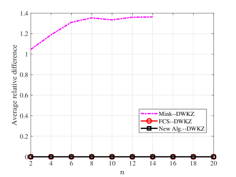
Figure 1: Average relative differences over $1000$ realizations

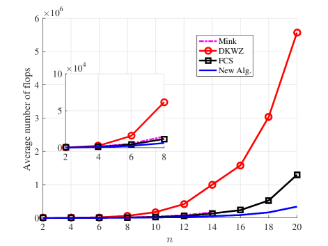
Figure 2: Average number of flops over $1000$ realizations

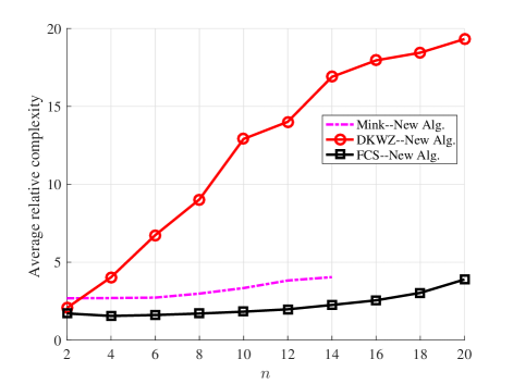
Figure 3: Average ratio of flops over $1000$ realizations

V Conclusion

In this paper, we have developed a novel efficient algorithm with an ${\mathcal{O}}(n^{2})$ memory complexity for optimally solving an SMP on an $n$-dimensional lattice, and theoretically showed its optimality. Theoretical complexity analysis showed that the new algorithm is $\Omega(n)$ times faster than the most efficient existing optimal algorithm with polynomial memory complexity. We have also asserted that it is faster than the most efficient existing algorithm with exponential memory complexity. Simulation results have also been provided to illustrate the optimality and efficiency of the proposed algorithm.

Appendix A Proof of Theorem 3

To prove Theorem 3, we need to introduce the following two lemmas. We begin with introducing the following Lemma which provides some properties of successive minima.

Lemma 1.

Suppose that there exist linearly independent vectors $\boldsymbol{b}_{1},\ldots,\boldsymbol{b}_{i}\in\mathcal{L}({\bar{\boldsymbol{R}}})=\{{\bar{\boldsymbol{R}}}\boldsymbol{a}|\boldsymbol{a}\in\mathbb{Z}^{n}\}$ satisfying $\|{\bar{\boldsymbol{R}}}\boldsymbol{b}_{j}\|_{2}=\lambda_{j}$ for $1\leq j\leq i$ with $1\leq i\leq n$. Then, they are the first $i$ columns of a solution of Problem 1.

Proof.

We assume $i<n$, otherwise, the lemma holds naturally. To prove the lemma, it suffices to show that there exist $\boldsymbol{b}_{i+1},\ldots,\boldsymbol{b}_{n}\in\mathcal{L}({\bar{\boldsymbol{R}}})$ such that $\boldsymbol{b}_{1},\ldots,\boldsymbol{b}_{n}$ are linearly independent and $\|{\bar{\boldsymbol{R}}}\boldsymbol{b}_{j}\|_{2}=\lambda_{j}$ for $i+1\leq j\leq n$. Let

$$\boldsymbol{b}_{i+1}= \operatorname*{arg\,min}_{\boldsymbol{b}\in S_{i}}\|{\bar{\boldsymbol{R}}}\boldsymbol{b}\|_{2},$$

$$\vdots$$

$$\boldsymbol{b}_{n}= \operatorname*{arg\,min}_{\boldsymbol{b}\in S_{n}}\|{\bar{\boldsymbol{R}}}\boldsymbol{b}\|_{2},$$

where

$$S_{i}= \{\boldsymbol{b}\in\mathbb{Z}^{n}\mbox{ such that }\boldsymbol{b},\boldsymbol{b}_{1},\ldots,\boldsymbol{b}_{i}\mbox{ are independent}\},$$

$$\quad\quad\quad\quad\quad\quad\quad\quad\vdots$$

$$S_{n}= \{\boldsymbol{b}\in\mathbb{Z}^{n}\mbox{ such that }\boldsymbol{b},\boldsymbol{b}_{1},\ldots,\boldsymbol{b}_{n-1}\mbox{ are independent}\}.$$

Then, by the proof of [10, Theorem 8], one can see that the above $\boldsymbol{b}_{i+1},\ldots,\boldsymbol{b}_{n}$ satisfy the above requirements. Note that since the solution of Problem 1 exists, $S_{i},\ldots,S_{n}$ are not empty sets. Hence, the lemma holds. ∎

By Lemma 1, we can get the following useful lemma.

Lemma 2.

Suppose that $\lambda_{i-1}({\bar{\boldsymbol{R}}})<\lambda_{i}({\bar{\boldsymbol{R}}})$ for some $2\leq i\leq n$, and $\boldsymbol{b}$ is the $i$-th column of a solution to the Problem 1. Let $\bar{\boldsymbol{b}}_{1},\ldots,\bar{\boldsymbol{b}}_{k}\in\mathcal{L}({\bar{\boldsymbol{R}}})$ be any linearly independent vectors which either satisfy that $\|{\bar{\boldsymbol{R}}}\bar{\boldsymbol{b}}_{j}\|_{2}<\lambda_{i}$ or $\|{\bar{\boldsymbol{R}}}\bar{\boldsymbol{b}}_{j}\|_{2}=\lambda_{i}$ and $\bar{\boldsymbol{b}}_{j}$ is not the $i$-th column of any solution of Problem 1, for $1\leq j\leq k$, then $\bar{\boldsymbol{b}}_{1},\ldots,\bar{\boldsymbol{b}}_{k},\boldsymbol{b}$ are linearly independent.

Proof.

Since $\boldsymbol{b}$ is the $i$-th column of a solution to Problem 1, there exists $\boldsymbol{b}_{1},\ldots,\boldsymbol{b}_{i-1}\in\mathbb{Z}^{n}$ such that $\boldsymbol{b}_{1},\ldots,\boldsymbol{b}_{i-1},\boldsymbol{b}$ are linearly independent and $\|{\bar{\boldsymbol{R}}}\boldsymbol{b}_{j}\|_{2}=\lambda_{j}<\lambda_{i}$ for $1\leq j\leq i-1$.

For any $1\leq j\leq k$, if $\|{\bar{\boldsymbol{R}}}\bar{\boldsymbol{b}}_{j}\|_{2}<\lambda_{i}$, then by the the definition of $\lambda_{i}$ and the assumption that $\lambda_{i-1}<\lambda_{i}$, $\bar{\boldsymbol{b}}_{j}$ is a linear combination of $\boldsymbol{b}_{1},\ldots,\boldsymbol{b}_{i-1}$. Otherwise, $\bar{\boldsymbol{b}}_{j},\boldsymbol{b}_{1},\ldots,\boldsymbol{b}_{i-1}$ are linearly independent, then according to $\|{\bar{\boldsymbol{R}}}\boldsymbol{b}_{\ell}\|_{2}\leq\lambda_{i-1}<\lambda_{i}$ for $1\leq\ell\leq i-1$ and $\|{\bar{\boldsymbol{R}}}\bar{\boldsymbol{b}}_{j}\|_{2}<\lambda_{i}$, one can obtain that $\lambda_{i}\leq\max\{\|{\bar{\boldsymbol{R}}}\boldsymbol{b}_{i-1}\|_{2},\|{\bar{\boldsymbol{R}}}\bar{\boldsymbol{b}}_{j}\|_{2}\}<\lambda_{i}$ which is impossible. If $\|\bar{\boldsymbol{b}}_{j}\|_{2}=\lambda_{i}$, since it is not the $i$-th column of any solution of Problem 1, by Lemma 1, $\bar{\boldsymbol{b}}_{j}$ is a linear combination of $\boldsymbol{b}_{1},\ldots,\boldsymbol{b}_{i-1}$.

Since $\bar{\boldsymbol{b}}_{1},\ldots,\bar{\boldsymbol{b}}_{k}$ are linearly independent, if $\bar{\boldsymbol{b}}_{1},\ldots,\bar{\boldsymbol{b}}_{k},\boldsymbol{b}$ are linearly dependent, then $\boldsymbol{b}$ is a linear combination of $\bar{\boldsymbol{b}}_{1},\ldots,\bar{\boldsymbol{b}}_{k}$, which combing with the above analysis imply that $\boldsymbol{b}$ is also a linear combination of $\boldsymbol{b}_{1},\ldots,\boldsymbol{b}_{i-1}$, contradicting the fact that $\boldsymbol{b}_{1},\ldots,\boldsymbol{b}_{i-1},\boldsymbol{b}$ are linearly independent. Thus, $\bar{\boldsymbol{b}}_{1},\ldots,\bar{\boldsymbol{b}}_{k},\boldsymbol{b}$ are linearly independent. ∎

In the following, we prove Theorem 3 by using Lemma 2.

Proof.

By Alg. 2, one can see that all the columns of $\boldsymbol{B}^{\star}$, which is a solver of Problem 1 and satisfies $b_{nj}^{\star}\geq 0$ and $b_{ij}^{\star}\geq 0$ if $\boldsymbol{b}_{i+1:n}^{\star}={\boldsymbol{0}}$ for $1\leq i\leq n-1$, $1\leq j\leq n$, can be searched by the algorithm. Thus, to show the theorem, it suffices to show that, during the process of Alg. 2, for $1\leq j\leq n$, the first $\boldsymbol{b}_{j}^{\star}$ (note that there may exist several $\boldsymbol{B}^{\star}$’s which are the solutions of Problem 1, and here “the first $\boldsymbol{b}_{j}^{\star}$” means the first vector that obtained by Alg. 2 and is the $j$-th column of a solver of Problem 1) will replace a column of $\boldsymbol{B}$ corresponding to the suboptimal solution when $\boldsymbol{b}_{j}^{\star}$ is obtained by Alg. 2 (in the following, we assume this $\boldsymbol{b}_{j}^{\star}$ is not a column of the $n\times n$ identity matrix, otherwise we only need to show the next step), and it will not be replaced by any vector $\boldsymbol{b}\in\mathbb{Z}^{n}$.

We first show the conclusion holds for $\boldsymbol{b}_{1}^{\star}$. Clearly, the matrix $\boldsymbol{B}$ corresponding to the suboptimal solution when the first $\boldsymbol{b}_{1}^{\star}$ is obtained satisfies $\|{\bar{\boldsymbol{R}}}\boldsymbol{b}_{j}\|_{2}>\|{\bar{\boldsymbol{R}}}\boldsymbol{b}^{\star}_{1}\|_{2}$ for $1\leq j\leq n$, thus, by Remark 1 and Alg. 2, the first $\boldsymbol{b}_{1}^{\star}$ will replace a column of $\boldsymbol{B}$. Moreover, as there is not any vector $\boldsymbol{b}\in\mathbb{Z}^{n}$ satisfying $\|{\bar{\boldsymbol{R}}}\boldsymbol{b}\|_{2}<\|{\bar{\boldsymbol{R}}}\boldsymbol{b}_{1}^{\star}\|_{2}$, by Alg. 2, $\boldsymbol{b}_{1}^{\star}$ will not be replaced by any vector $\boldsymbol{b}\in\mathbb{Z}^{n}$ which is not the $j$-th column of any solution of Problem 1.

In the following, we show the conclusion holds for the first $\boldsymbol{b}_{j}^{\star}$ for any $2\leq j\leq n$ with Lemma 2 by considering two cases: $\lambda_{j-1}<\lambda_{j}$ and $\lambda_{j-1}=\lambda_{j}$.

Suppose that $\lambda_{j-1}<\lambda_{j}$. Let $\boldsymbol{B}$ be the suboptimal solution when the first $\boldsymbol{b}_{j}^{\star}$ is obtained. Since $\boldsymbol{B}$ is full-rank and $\boldsymbol{b}_{j}^{\star}$ is the first vector that it is the $j$-th column of a solution of Problem 1, by Lemma 2 and Alg. 2, $\boldsymbol{b}_{j}^{\star}$ will replace a column of $\boldsymbol{B}$. Moreover, by Lemma 2, all the linearly independent vectors $\boldsymbol{b}\in\mathbb{Z}^{n}$ either satisfy that $\|{\bar{\boldsymbol{R}}}\boldsymbol{b}\|_{2}<\|{\bar{\boldsymbol{R}}}\boldsymbol{b}_{j}^{\star}\|_{2}$ or $\|{\bar{\boldsymbol{R}}}\boldsymbol{b}\|_{2}=\|{\bar{\boldsymbol{R}}}\boldsymbol{b}_{j}^{\star}\|_{2}$ and $\boldsymbol{b}$ is not the $i$-th column of any solution to Problem 1 are linearly independent with $\boldsymbol{b}_{j}^{\star}$, thus by Alg. 2, $\boldsymbol{b}_{j}^{\star}$ will not be replaced by any vector $\boldsymbol{b}\in\mathbb{Z}^{n}$ which is not the $j$-th column of any solution of Problem 1.

Suppose that $\lambda_{j-1}=\lambda_{j}$. We consider two cases: all the first $j-1$ successive minima of lattice $\mathcal{L}({\bar{\boldsymbol{R}}})$ are equal, and at least two of the successive minima of lattice $\mathcal{L}({\bar{\boldsymbol{R}}})$ are different.

We first consider the first case. In this case, $\lambda_{1}=\ldots=\lambda_{i}$. By the above analysis, Alg. 2 can find the first $\boldsymbol{b}_{1}^{\star}$, use it to replace the first column of the suboptimal solution corresponding to $\boldsymbol{b}_{1}^{\star}$, and will not be replaced by any other vectors. Since $\lambda_{2}=\lambda_{1}$, there exists at least one $\boldsymbol{b}\in\mathbb{Z}^{n}$ such that $\|{\bar{\boldsymbol{R}}}\boldsymbol{b}\|_{2}=\|{\bar{\boldsymbol{R}}}\boldsymbol{b}_{1}^{\star}\|_{2}$ and ${\bar{\boldsymbol{R}}}\boldsymbol{b}_{1}^{\star}$ and ${\bar{\boldsymbol{R}}}\boldsymbol{b}$ are linearly independent. Thus, the first $\boldsymbol{b}_{2}^{\star}$, will replace the second column of the suboptimal solution corresponding to this vector. Since there is not any vector $\boldsymbol{b}\in\mathbb{Z}^{n}$ satisfying $\|{\bar{\boldsymbol{R}}}\boldsymbol{b}\|_{2}<\lambda_{2}=\lambda_{1}$, by Alg. 2, $\boldsymbol{b}_{2}^{\star}$ will not be replaced by any vector $\boldsymbol{b}\in\mathbb{Z}^{n}$. Similarly, one can show that the first $\boldsymbol{b}_{j}^{\star}$ will replace a column of $\boldsymbol{B}$ corresponding to the suboptimal solution when it is obtained. Moreover, since there is not any vector $\boldsymbol{b}\in\mathbb{Z}^{n}$ satisfying $\|{\bar{\boldsymbol{R}}}\boldsymbol{b}\|_{2}<\lambda_{1}=\lambda_{i}$, by Alg. 2, $\boldsymbol{b}_{j}^{\star}$ will not be replaced by any other vector $\boldsymbol{b}\in\mathbb{Z}^{n}$.

We then consider the second case, and let (if $j\geq 3$) $k=\operatorname*{arg\,min}_{1\leq i\leq j-2}\lambda_{i}<\lambda_{i+1}.$ By the above proof, one can see that Alg. 2 can find $\boldsymbol{b}_{1}^{\star},\ldots,\boldsymbol{b}_{k}^{\star}$, use them to replace the first $k$ columns of the suboptimal solution corresponding to them iteratively, and will not replace them with any other vectors. Since $\lambda_{k}<\lambda_{k+1}$, the conclusion holds clearly for $\boldsymbol{b}_{k+1}^{\star}$. Similarly and iteratively, one can show that $\boldsymbol{b}_{j}^{\star}$ will replace a column of $\boldsymbol{B}$ corresponding to the suboptimal solution when it is obtained, and it will not be replaced by any vector $\boldsymbol{b}\in\mathbb{Z}^{n}$ which is not the $j$-th column of any solution of Problem 1. ∎

References

• [1] J. Zhan, B. Nazer, U. Erez, and M. Gastpar, “Integer-forcing linear receivers: A new low-complexity MIMO architecture,” in Proc. IEEE 72th Vehicular Technology Conference (VTC Fall), 2010, pp. 1–5.
• [2] ——, “Integer-forcing linear receivers,” IEEE Trans. Inf. Theory, vol. 60, no. 12, pp. 7661–7685, Dec. 2014.
• [3] K. V. Vardhan, S. K. Mohammed, A. Chockalingam, and B. S. Rajan, “A low-complexity detector for large MIMO systems and multicarrier CDMA systems,” IEEE J. Sel. Areas Commun., vol. 26, no. 3, pp. 473–485, April 2008.
• [4] R. C. D. Lamare and R. Sampaio-Neto, “Minimum mean-squared error iterative successive parallel arbitrated decision feedback detectors for DS-CDMA systems,” IEEE Trans. Commun, vol. 56, no. 5, pp. 778–789, May 2008.
• [5] S. Yang, T. Lv, R. G. Maunder, and L. Hanzo, “Unified bit-based probabilistic data association aided MIMO detection for high-order QAM constellations,” IEEE Trans. Veh. Technol., vol. 60, no. 3, pp. 981–991, March 2011.
• [6] T. Hwang, Y. Kim, and H. Park, “Energy spreading transform approach to achieve full diversity and full rate for MIMO systems,” IEEE Trans. Signal Process., vol. 60, no. 12, pp. 6547–6560, Dec 2012.
• [7] P. Li and R. C. D. Lamare, “Adaptive decision-feedback detection with constellation constraints for MIMO systems,” IEEE Trans. Veh. Technol., vol. 61, no. 2, pp. 853–859, Feb. 2012.
• [8] R. C. de Lamare, “Adaptive and iterative multi-branch MMSE decision feedback detection algorithms for multi-antenna systems,” IEEE Trans. Wirel. Commun., vol. 12, no. 10, pp. 5294–5308, Oct. 2013.
• [9] A. G. D. Uchoa, C. T. Healy, and R. C. de Lamare, “Iterative detection and decoding algorithms for MIMO systems in block-fading channels using LDPC codes,” IEEE Trans. Veh. Technol., vol. 65, no. 4, pp. 2735–2741, April 2016.
• [10] C. Feng, D. Silva, and F. R. Kschischang, “An algebraic approach to physical-layer network coding,” IEEE Trans. Inf. Theory, vol. 59, no. 11, pp. 7576–7596, Nov. 2013.
• [11] Y. Tan and X. Yuan, “Compute-compress-and-forward: Exploiting asymmetry of wireless relay networks,” IEEE Trans. Signal Process., vol. 64, no. 2, pp. 511–524, Jan. 2016.
• [12] L. Wei and W. Chen, “Integer-forcing linear receiver design over MIMO channels.” in Proc. IEEE Global Commun. Conf (GLOBECOM), 2012, pp. 3560–3565.
• [13] A. Mejri and G. R. B. Othman, “Practical implementation of integer forcing linear receivers in MIMO channels,” in Proc. IEEE 78th Vehicular Technology Conference (VTC Fall), Sept. 2013, pp. 1–5.
• [14] L. Ding, K. Kansanen, Y. Wang, and J. Zhang, “Exact SMP algorithms for integer-forcing linear MIMO receivers,” IEEE Trans. Wireless Commun., vol. 14, no. 12, pp. 6955–6966, Dec. 2015.
• [15] R. F. Fischer, M. Cyran, and S. Stern, “Factorization approaches in lattice-reduction-aided and integer-forcing equalization,” in Proc. Int. Zurich Seminar on Communications, Zurich, Switzerland, 2016.
• [16] A. Lenstra, H. Lenstra, and L. Lovász, “Factoring polynomials with rational coefficients,” Math. Ann., vol. 261, no. 4, pp. 515–534, 1982.
• [17] C. Schnorr and M. Euchner, “Lattice basis reduction: improved practical algorithms and solving subset sum problems,” Math Program, vol. 66, no. 1-3, pp. 181–191, Aug. 1994.
• [18] E. Agrell, T. Eriksson, A. Vardy, and K. Zeger, “Closest point search in lattices,” IEEE Trans. Inf. Theory, vol. 48, no. 8, pp. 2201–2214, Aug. 2002.
• [19] L. Wei and W. Chen, “Integer-forcing linear receiver design with slowest descent method,” IEEE Trans. Wireless Commun., vol. 12, no. 6, pp. 2788–2796, June 2013.
• [20] A. Sakzad, J. Harshan, and E. Viterbo, “Integer-forcing MIMO linear receivers based on lattice reduction,” IEEE Trans. Wireless Commun., vol. 12, no. 10, pp. 4905–4915, Oct. 2013.
• [21] S. Lyu and C. Ling, “Boosted KZ and LLL algorithms,” IEEE Trans. Signal Process., vol. 65, no. 18, pp. 4784–4796, Sept. 2017.
• [22] J. Wen, L. Li, X. Tang, W. H. Mow, and C. Tellambura, “An efficient optimal algorithm for integer-forcing linear MIMO receivers design,” in Proc. IEEE Int. Conf. Commun. (ICC), May 2017, pp. 1–6.
• [23] J. Wen and X.-W. Chang, “On the KZ reduction,” to appear in IEEE Trans. Inf. Theory, 2018.
• [24] G. Golub and C. Van Loan, “Matrix computations, 4th,” Johns Hopkins, 2013.
• [25] X.-W. Chang, J. Wen, and X. Xie, “Effects of the LLL reduction on the success probability of the Babai point and on the complexity of sphere decoding,” IEEE Trans. Inf. Theory, vol. 59, no. 8, pp. 4915–4926, Aug. 2013.
• [26] J. Wen, C. Tong, and S. Bai, “Effects of some lattice reductions on the success probability of the zero-forcing decoder,” IEEE Commun. Lett., vol. 20, no. 10, pp. 2031–2034, Oct. 2016.
• [27] J. Wen and X.-W. Chang, “The success probability of the Babai point estimator and the integer least squares estimator in box-constrained integer linear models,” IEEE Trans. Inf. Theory, vol. 63, no. 1, pp. 631–648, Jan. 2017.
• [28] C. P. Schnorr, “A hierarchy of polynomial time lattice basis reduction algorithms,” Theor. Comput. Sci., vol. 53, pp. 201–224, 1987.
• [29] X.-W. Chang and Q. Han, “Solving box-constrained integer least squares problems,” IEEE Trans. Wireless Commun., vol. 7, no. 1, pp. 277–287, Jan. 2008.
• [30] T. Cui, S. Han, and C. Tellambura, “Probability-distribution-based node pruning for sphere decoding,” IEEE Trans. Veh. Technol., vol. 62, no. 4, pp. 1586–1596, May 2013.
• [31] J. Wen, B. Zhou, W. H. Mow, and X.-W. Chang, “An efficient algorithm for optimally solving a shortest vector problem in compute-and-forward design,” IEEE Trans. Wireless Commun., vol. 15, no. 10, pp. 6541–6555, Oct. 2016.
• [32] C. Ling, W. H. Mow, and N. Howgrave-Graham, “Reduced and fixed-complexity variants of the LLL algorithm for communications,” IEEE Trans. Commun., vol. 61, no. 3, pp. 1040–1050, Mar. 2013.
• [33] B. Hassibi and H. Vikalo, “On the sphere-decoding algorithm I. Expected complexity,” IEEE Trans. Signal Process., vol. 53, no. 8, pp. 2806–2818, Aug. 2005.
• [34] P. M. Gruber and J. M. Wills, Eds., Handbook of convex geometry.   North-Holland, Amsterdam, 1993.
• [35] A. Banihashemi and A. K. Khandani, “On the complexity of decoding lattices using the korkin-zolotarev reduced basis,” IEEE Trans. Inf. Theory, vol. 44, no. 1, pp. 162–171, Jan. 1998.
• [36] H. Minkowski, “Geometrie der zahlen (2 vol.),” Teubner, Leipzig, vol. 1910, 1896.
• [37] W. Zhang, S. Qiao, and Y. Wei, “HKZ and Minkowski reduction algorithms for lattice-reduction-aided MIMO detection,” IEEE Trans. Signal Process., vol. 60, no. 11, pp. 5963–5976, Nov. 2012.
• [38] J. Wen and X.-W. Chang, “A modified KZ reduction algorithm,” in 2015 IEEE Int. Symp. Inf. Theory (ISIT), 2015, pp. 451–455.