Functional Asynchronous Networks: Factorization of Dynamics and Function

Abstract

In this note we describe the theory of functional asynchronous networks and one of the main results, the Modularization of Dynamics Theorem, which for a large class of functional asynchronous networks gives a factorization of dynamics in terms of constituent subnetworks. For these networks we can give a complete description of the network function in terms of the function of the events comprising the network and thereby answer a question originally raised by Alon in the context of biological networks.

I Introduction

Kastan & Alon KU identify and describe the configurations of relatively simple and small subnetworks that occur more frequently in biological networks than would be the case if the network were random. They refer to these subnetworks as network motifs. Later, in his 2007 book on systems biology Alon , Alon makes the following comment

“Ideally, we would like to understand the dynamics of the entire network based on the dynamics of the individual building blocks.” (Alon (Alon, , page 27).)

The underlying premise behind this comment is that a modular, or engineering, approach to network dynamics is feasible. Identify building blocks, connect together to form networks and then describe dynamical properties of the resulting network in terms of the dynamics of its components. This approach works well in linear systems theory, where a superposition principle holds, or in, for example, the study of synchronization in weakly coupled systems of nonlinear approximately identical oscillators where network dynamics can be closely related to the dynamics of individual nodes (oscillators).

However, from the perspective of a mathematician or physicist, Alon’s comment seems unhelpful for the study of dynamics of heterogenous networks modelled by systems of nonlinear ODEs. This is a well-known issue in complex systems LLK . Yet engineers do couple gadgets together to make more complex systems and so it is natural to ask if it is possible to reconcile these viewpoints.

In this note, we outline some of the basic ideas involved in an approach to network dynamics based on what we call asynchronous networks. We allow for features seen in networks from technology, engineering, and biology (for example, neuroscience or gene transcription networks). Network dynamics can involve a mix of distributed and decentralized control, adaptivity, event driven dynamics, switching, varying network topology and hybrid dynamics. Typically network dynamics will be piecewise smooth, time-irreversible, nodes may stop and later restart, and there may be no intrinsic global time. Significantly, many of these networks have a function: transportation networks bring people and goods from one point to another, neural networks may perform pattern recognition or computation, etc. Our goal is to address Alon’s comment in the context of functional asynchronous networks. Specifically, we describe a factorization of dynamics theorem where it is possible to describe the function of a large class of functional asynchronous networks in terms of the function of constituent subnetworks. As this article is only intended to be an introduction, we work always with the simplest examples and models and omit technical details. We refer the reader to BF1 ; BF2 for greater detail, generality and proofs.

II Examples and properties of asynchronous networks

We briefly describe some characteristic examples of asynchronous networks (we refer to (BF1, , §3) for more detail).

II.1 Threaded & parallel computation

In threaded or parallel computation, computation is broken into blocks or ‘threads’ which are then computed independently of each other at a speed that depends on the clock rates of the individual processors. As the computation proceeds, threads may need to exchange information with other threads. This process involves stopping and synchronizing (updating) the thread states. Each thread may have to stop and wait for other threads to complete their computations before it can continue with its own computation. Each thread has its own clock (determined by its associated processor). If threads run on separate processors, threads will be unaware of the clock times of other threads except during the stopping and synchronization events.

II.2 Production and transport networks

We give a simple detailed example of a transport network in section IV. In production networks, parts, compounds, etc. are repeatedly built and combined as part of a production process leading to the desired item (for example, a car or protein). In particular, there is variation in both connection structure, typically intermittent, and in the set of nodes (nodes may be combined or decomposed).

II.3 Power grid models

A power grid consists of a network of various types of generators and loads connected by transmission lines. A microgrid is a local network, capable of existing independently of the main power grid, and typically powered by renewable energy sources (for example, solar or wind power). Critical questions involve the stability of the power grid in case of loss of a transmission line or generator (variation in network structure), and control and stability issues related to combining and separation (islanding) of a large set of microgrids from the main power grid.

II.4 Thresholds, spiking models and adaptation

Many mathematical models from engineering and biology incorporate thresholds. For networks, when a node attains a threshold, there are often changes (addition, deletion, weights) in connections to another nodes. For networks of neurons, reaching a threshold can result in a neuron firing (spiking) and short term connections to other neurons (for transmission of the spike). For learning mechanisms, such as Spike-Timing Dependent Plasticity (STDP) Ge relative timings (the order of firing) are crucial GK ; CD ; MDG and so each neuron, or connection between a pair of neurons, comes with a ‘local clock’ that governs the adaptation in STDP. In general, networks with thresholds, spiking and adaptation provide characteristic examples of asynchronous networks where dynamics is piecewise smooth and hybrid – a mix of continuous and discrete dynamics.

II.5 Properties of asynchronous networks

We summarize some of the characteristic features of asynchronous networks as revealed in the examples above.

1. Variable network structure and dependencies between nodes. Changes depend on the state of the system or are given by a stochastic process.

2. Synchronization events associated with stopping or waiting states of nodes.

3. Order of events may depend on the initialization of the system or stochastic effects.

4. Dynamics is only piecewise smooth and there may be a mix of continuous and discrete dynamics.

5. Aspects involving function, adaptation and control.

6. Evolution only defined for forward time – systems are not time reversible.

III Asynchronous networks: formalism

We use the notational conventions that $\mathbf{k}=\{1,\ldots,k\}$ and $\mathbf{k}^{\bullet}=\mathbf{k}\cup\{0\}$, $k\in\mbox{$\mathbb{N}$}$. Let $\mbox{$\mathbb{R}$}_{+}=\{x\in\mbox{$\mathbb{R}$}\mbox{$\;|\;$}x>0\}$.

Assume given a network with $k$ nodes, $N_{1},\ldots,N_{k}$. Suppose that $N_{i}$ has associated phase space $M_{i}$, $i\in\mathbf{k}$. Set $\mathbf{M}=\prod_{i\in\mathbf{k}}M_{i}$ – the network phase space. A vector field $\mathbf{f}$ on $\mathbf{M}$ is a network vector field.

Stopping, waiting, and synchronization are a feature of asynchronous networks. If nodes are stopped or partially stopped, node dynamics will be constrained to subsets of node phase space. We codify this situation by introducing a constraining node $N_{0}$ that, when connected to $N_{i}$, implies that dynamics on $N_{i}$ is constrained. Set $\mathcal{N}=\{N_{0},\ldots,N_{k}\}$.

III.1 Connection structures; admissible vector fields

Interactions between distinct nodes in the network are given by the network graph. Connections $N_{j}\mbox{$\rightarrow$}N_{i}$ encode dependencies if $i,j\in\mathbf{k}$, and constraints if $j=0$, $i\in\mathbf{k}$.

A connection structure $\alpha$ is a directed network graph on the nodes $\mathcal{N}$ such that for all $i\in\mathbf{k}$, $j\in\mathbf{k}^{\bullet}$, $i\neq j$, there is at most one directed connection $N_{j}\mbox{$\rightarrow$}N_{i}$. We do not allow self-loops or connections to the constraining node $N_{0}$.

An $\alpha$-admissible vector field $\mathbf{f}^{\alpha}$ is a network vector field with dependencies given by $\alpha$. If $N_{j}\mbox{$\rightarrow$}N_{i}\notin\alpha$, $i\neq j$, then $\mathbf{f}^{\alpha}$ does not depend on $x_{j}\in M_{j}$ (and conversely, see (BF1, , §2)).

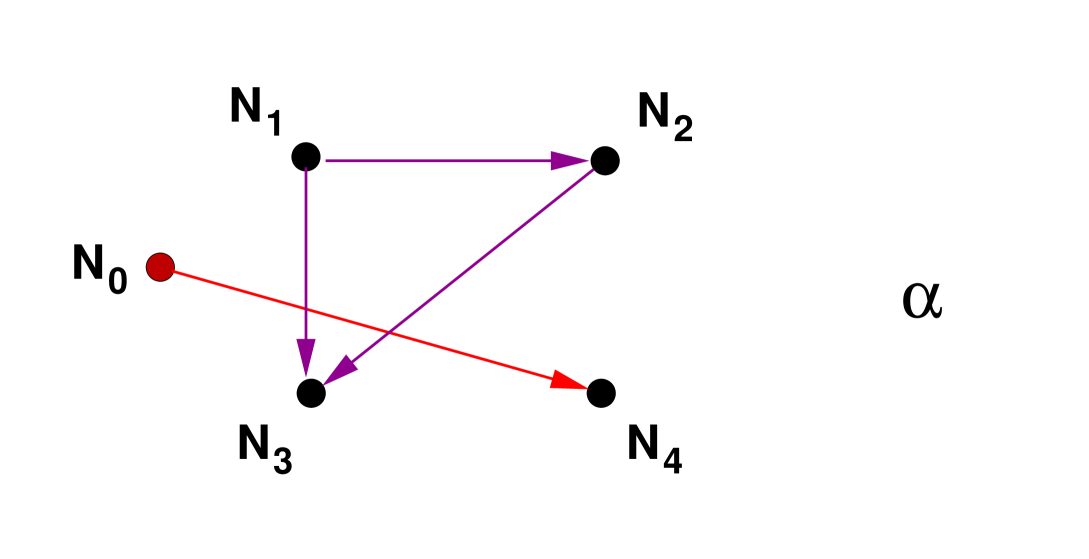
Figure 1: Construction structure on $\{N_{0},N_{1},N_{2},N_{3},N_{4}\}$.

Referring to figure 1, suppose $\mathbf{f}^{\alpha}=(f_{1}^{\alpha},\ldots,f_{4}^{\alpha})$ is $\alpha$-admissible. For $\mathbf{X}=({\mathbf{x}}_{1},{\mathbf{x}}_{2},{\mathbf{x}}_{3},{\mathbf{x}}_{4})\in\mathbf{M}$, we have

$$f_{1}^{\alpha}(\mathbf{X})=f_{1}({\mathbf{x}}_{1}),\;f_{2}^{\alpha}(\mathbf{X})=f_{2}({\mathbf{x}}_{2};{\mathbf{x}}_{1})\;$$

$$f_{3}^{\alpha}(\mathbf{X})=f_{3}({\mathbf{x}}_{3};{\mathbf{x}}_{1},{\mathbf{x}}_{2}),\;f_{4}^{\alpha}(\mathbf{X})=0,$$

where here we have assumed that the constraint $N_{0}\mbox{$\rightarrow$}N_{4}$ results in $N_{4}$ being stopped.

A generalized connection structure $\mathcal{A}$ is a (nonempty) set of connection structures on $\mathcal{N}$.

An $\mathcal{A}$-structure $\mathcal{F}$ is a set $\mathcal{F}=\{\mathbf{f}^{\alpha}\mbox{$\;|\;$}\alpha\in\mathcal{A}\}$ of network vector fields such that each $\mathbf{f}^{\alpha}\in\mathcal{F}$ is $\alpha$-admissible.

III.2 The event map and asynchronous networks

Suppose that $\mathcal{A}$ is a generalized connection structure and $\mathcal{F}$ is an $\mathcal{A}$-structure.

Interactions between nodes in asynchronous networks may be state dependent or change over time (stochastically). Here we only consider state dependence.

We handle interactions and constraints using an event map $\mathcal{E}:\mathbf{M}\mbox{$\rightarrow$}\mathcal{A}$.

The quadruple $\mathfrak{N}=(\mathcal{N},\mathcal{A},\mathcal{F},\mathcal{E})$ defines an asynchronous network. Dynamics on $\mathfrak{N}$ is given by the state dependent network vector field $\mathcal{F}$ defined by

$$\mathbf{F}(\mathbf{X})=\mathbf{f}^{\mathcal{E}(\mathbf{X})}(\mathbf{X}),\;\mathbf{X}\in\mathbf{M}.$$ (III.1)

Remark 1.

We refer to (BF1, , §4.7) for the definition of an integral curve for III.1 and note that the definition we use is different from that used in Filippov systems Fil ; BBCK . Under simple conditions on the event map (BF1, , §§4.7, 4.8), it can be shown that if $\mathbf{M}$ is compact then for each $\mathbf{X}\in\mathbf{M}$ there is a unique piecewise smooth integral curve $\Phi_{\mathbf{X}}:[0,\infty)\mbox{$\rightarrow$}\mathbf{M}$ with initial condition $\mathbf{X}$ and corresponding semiflow $\Phi:\mathbf{M}\times\mbox{$\mathbb{R}$}_{+}\mbox{$\rightarrow$}\mathbf{M}$. In general, $\Phi$ will not be continuous as a function of $\mathbf{X}\in\mathbf{M}$.

IV A simple transport example

Figure 2: A single track railway line with a passing loop.

We consider a single track railway line joining stations marked $S_{1},S_{2}$ in figure 2. Suppose there is a passing loop at $L$. Trains, marked $T_{1}$ and $T_{2}$ in figure 2, start from stations $S_{1}$ and $S_{2}$ respectively and proceed towards the opposite station. There is no central control or communication between the train drivers except when both trains are in the passing loop. We further assume that both drivers are running a nonlinear oscillator. When a train enters the passing loop it stops. When both trains are in the passing loop, the drivers cross couple their nonlinear oscillators. In order for a train to leave the passing loop, two conditions must be satisfied.

1. Both trains must be in the passing loop.

2. The two nonlinear oscillators must be phase synchronized to within $\varepsilon$ where $0<\varepsilon\ll\pi$.

We model this setup using an asynchronous network with two nodes – corresponding to the two trains. The phase space for train $T_{i}$ will be $M_{i}=[-a,b]\times\mathbb{T}$, $i\in\mathbf{2}$ ($\mathbb{T}=\mbox{$\mathbb{R}$}/2\pi\mbox{$\mathbb{Z}$}$), where the interval $[-a,b]$ models the line joining $S_{1}$ to $S_{2}$, $S_{1}$ has coordinate $-a<0$, $S_{2}$ has coordinate $b>0$, The passing loop $L$ will be at $x=0$, and $\mathbb{T}$ will be the phase space for the nonlinear oscillator.

Assume train motion given by $V_{1},V_{2}$ where $V_{1}(x)>0>V_{2}(x)$ $x\in[-a,b]$. Note that neither $V_{1}$ or $V_{2}$ can be zero anywhere on $[-a,b]$ otherwise the trains will never both reach their destination stations in finite time.

We define four connection structures.

$$\alpha_{i} = N_{0}\mbox{$\rightarrow$}N_{i},\;i\in\mathbf{2}\;(\mbox{$T_{i}$ stopped})$$

$$\beta = N_{0}\mbox{$\rightarrow$}N_{1}\leftrightarrow N_{2}\leftarrow N_{0}(\mbox{stopped \& cross coupled})$$

$${\emptyset} =$$ Empty connection structure

Let $\mathcal{A}=\{\alpha_{1},\alpha_{2},\beta,{\emptyset}\}$ be the associated generalized connection structure.

Model the uncoupled oscillator dynamics for train $T_{i}$ by $\dot{\theta}_{i}=\omega$, where $\omega>0$, and the coupled dynamics by the Kuramoto phase oscillator system

$$\dot{\theta}_{1} = \omega+\sin(\theta_{2}-\theta_{1})$$

$$\dot{\theta}_{2} = \omega+\sin(\theta_{1}-\theta_{2})$$

It remains to define the admissible vector fields and event map that give the required dynamics for this example. As admissible vector fields (on $([-a,b]\times\mathbb{T})^{2}$) we take

$$\mathbf{f}^{\emptyset}\, = ((V_{1},g),(V_{2},g)),$$

$$\mathbf{f}^{\alpha_{1}} = ((0,g),(V_{2},g)),\;(T_{1}\;\mbox{stopped},\;T_{2}\;\mbox{running})$$

$$\mathbf{f}^{\alpha_{2}} = ((V_{1},g),(0,g)),\;(T_{2}\;\mbox{stopped},\;T_{1}\;\mbox{running})$$

$$\mathbf{f}^{\beta}\, = ((0,G_{1}),(0,G_{2})),\;(T_{1},T_{2}\;\mbox{stopped \& cross coupled})$$

We define the event map by

$$\mathcal{E}(\mathbf{X},\bm{\theta}) = \alpha_{1},\;x_{1}=0,x_{2}>0$$

$$= \alpha_{2},\;x_{1}<0,x_{2}=0$$

$$= \beta,\;x_{1}=x_{2}=0,\;|\theta_{1}-\theta_{2}|>\varepsilon$$

$$= {\emptyset},\;\mbox{otherwise}$$

Finally, dynamics are given by the network vector field

$$F(\mathbf{X},\bm{\theta})=\mathbf{f}^{\mathcal{E}(\mathbf{X},\bm{\theta})}(\mathbf{X},\bm{\theta}).$$ (IV.2)

We leave it as an easy exercise for the reader to check that if $T_{i}$ is initialized at $(x_{i}(0),\theta_{i}(0))\in[-a,b]\times\mathbb{T}$, $i\in\mathbf{2}$, where $x_{1}(0)\leq 0\leq x_{2}(0)$, then IV.2 has a well defined integral curve $\varphi:\mbox{$\mathbb{R}$}_{+}\mbox{$\rightarrow$}([-a,b]\times\mathbb{T})^{2}$, with specified initial condition, that gives the correct dynamics for the passing loop problem.

Remark 2.

The passing loop gives an example of a simple functional asynchronous network. The function is for the trains to go from one station to the opposite station in finite time. Observe that for this example there is the possibility of a dynamical deadlock: if the trains start at the same time and if $\theta_{1}(0)=\theta_{2}(0)+\pi$, then the coupled phase oscillators will never phase synchronize – $\theta_{1}(t)=\theta_{2}(t)+\pi$ for all $t\in\mbox{$\mathbb{R}$}_{+}$ – and so the trains will never exit the passing loop. We refer to (BF2, , §§2,3) for more details on deadlocks in functional asynchronous networks.

V Functional asynchronous networks

We follow the notational conventions of section III and let $\mathfrak{N}=(\mathcal{N},\mathcal{A},\mathcal{F},\mathcal{E})$ denote an asynchronous network. We assume that $\mathfrak{N}$ has associated semiflow

$$\Phi=(\Phi_{1},\ldots,\Phi_{k}):\mathbf{M}\times\mbox{$\mathbb{R}$}_{+}\mbox{$\rightarrow$}\mathbf{M}.$$

Suppose that we are given initialization and termination sets $\mathbb{I},\mathbb{F}\subset\mathbf{M}$ where

$$\mathbb{I}=\prod_{i\in\mathbf{k}}\mathbb{I}_{i},\quad\mathbb{F}=\prod_{i\in\mathbf{k}}\mathbb{F}_{i},$$

Typically, $\mathbb{I}_{i},\mathbb{F}_{i}\subset M_{i}$ will be closed disjoint hypersurfaces that separate $M_{i}$ into three connected components, $i\in\mathbf{k}$. That is, $M_{i}=M_{i}^{-}\cup M_{i}^{0}\cup M_{i}^{+}$ where $M_{i}^{-}\cap M_{i}^{+}=\emptyset$ and

$$M_{i}^{-}\cap M_{i}^{0}=\partial M_{i}^{-}=\mathbb{I}_{i},\quad M_{i}^{0}\cap M_{i}^{+}=\partial M_{i}^{+}=\mathbb{F}_{i}.$$

We call $\mathbf{N}=(\mathfrak{N},\mathbb{I},\mathbb{F})$ a functional asynchronous network. The network function is getting from $\mathbb{I}$ to $\mathbb{F}$ and is expressed by the transition and timing functions

$$G_{0}:\mathcal{D}\subset\mathbb{I}\mbox{$\rightarrow$}\mathbb{F},\quad\mathbf{S}:\mathcal{D}\subset\mathbb{I}\mbox{$\rightarrow$}\mbox{$\mathbb{R}$}_{+}^{k}.$$

That is, if $\mathbf{X}\in\mathcal{D}$, then for all $i\in\mathbf{k}$ there exists $S_{i}\in\mbox{$\mathbb{R}$}_{+}^{k}$ such that

$$\Phi_{i}(\mathbf{X},S_{i}) \in \mathbb{F}_{i},\quad\Phi_{i}(\mathbf{X},t)\notin\mathbb{F}_{i},t<S_{i},$$

$$\mathbf{S}(\mathbf{X}) = (S_{1},\ldots,S_{k}),$$

Example 1.

For the passing loop example discussed in the previous section, we take $\mathbb{I}_{1}=M_{1}^{-}=M_{2}^{+}=\mathbb{F}_{2}=\{-a\}\times\mathbb{T}$, $\mathbb{F}_{1}=M_{1}^{+}=M_{2}^{+}=\mathbb{I}_{2}=\{b\}\times\mathbb{T}$. In this case, there is the implicit assumption that trains stop when they reach their termination set. Equally well, we could take $M_{i}=\mbox{$\mathbb{R}$}\times\mathbb{T}$ so that $M_{1}^{-}=(-\infty,a]\times\mathbb{T}$ etc. (see also (BF2, , §3)). Finally, observe that $\mathcal{D}=\{((-a,\theta_{1}),(b,\theta_{2}))\mbox{$\;|\;$}|\theta_{1}-\theta_{2}|\neq\pi\}$.

More generally, we allow for general initialization times and define generalized transition and timing functions

$$G:\widehat{\mathcal{D}}\subset\mathbb{I}\times\mbox{$\mathbb{R}$}_{+}^{k}\mbox{$\rightarrow$}\mathbb{F},\quad\widehat{\mathbf{S}}:\widehat{\mathcal{D}}\subset\mathbb{I}\times\mbox{$\mathbb{R}$}_{+}^{k}\mbox{$\rightarrow$}\mbox{$\mathbb{R}$}_{+}^{k}.$$

We refer to (BF2, , §3.4) for details. For our main result, it is required that the network has a generalized transition and timing functions with $\widehat{\mathcal{D}}=\mathbb{I}\times\mbox{$\mathbb{R}$}_{+}^{k}$.

V.1 Functional networks built from events

In figure 3 we show a nine node functional asynchronous network that is built from the eight “events” $\mathbf{P}^{a},\ldots,\mathbf{P}^{h}$.

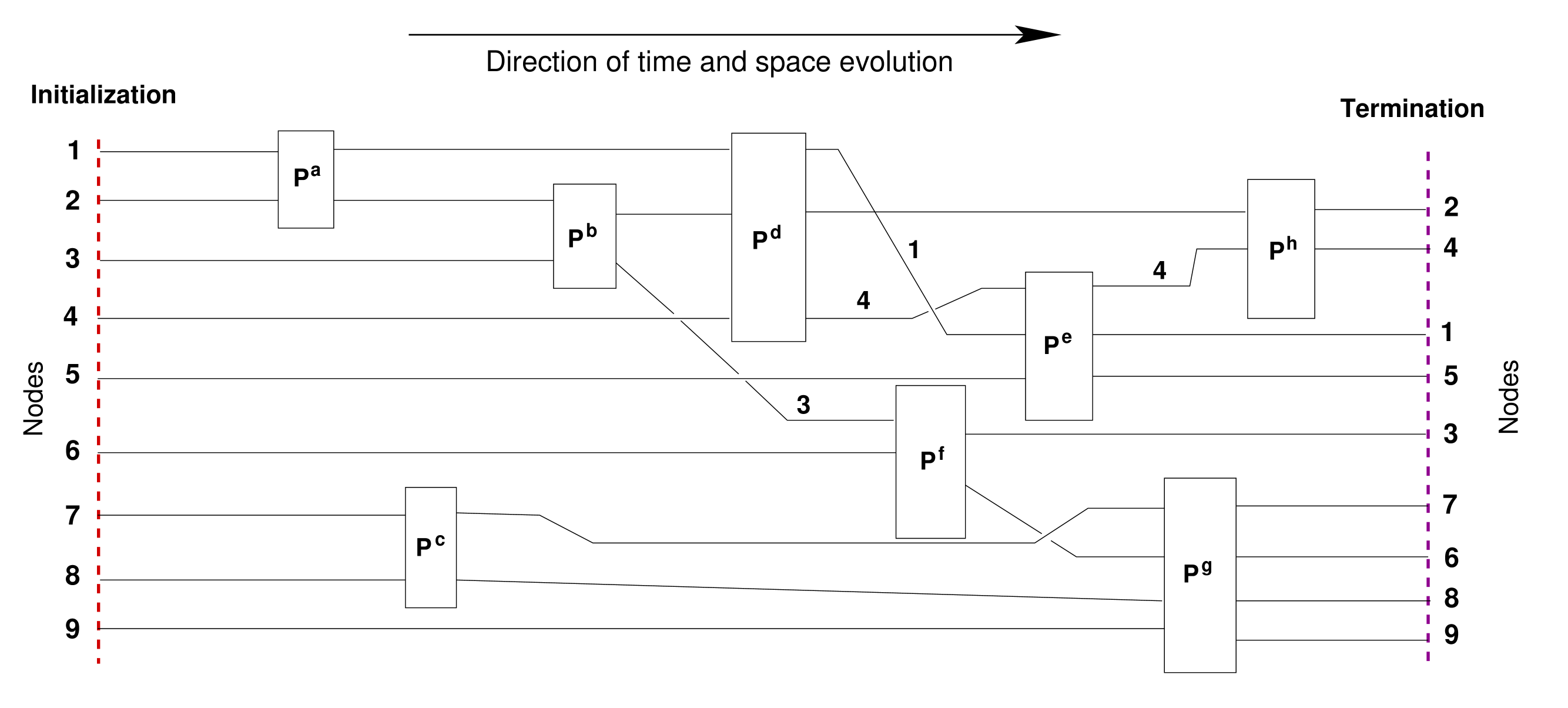
Figure 3: A spatiotemporal decomposition of a functional asynchronous network

The initialization and termination sets are indicated on the left and right sides of the figure respectively. The events signify regions of phase space where there can be (state dependent) interaction between nodes. For example, the event labelled $\mathbf{P}^{g}$ involves interaction between nodes $N_{6}$, $N_{7}$, $N_{8}$, and $N_{9}$. Observe that there is only a partially ordered temporal structure on the events. Thus, the event $\mathbf{P}^{g}$ must occur after $\mathbf{P}^{f}$ but can occur before or after event $\mathbf{P}^{h}$.

V.2 Building blocks

In figure 4 we represent a basic building block with the same number of inputs and outputs.

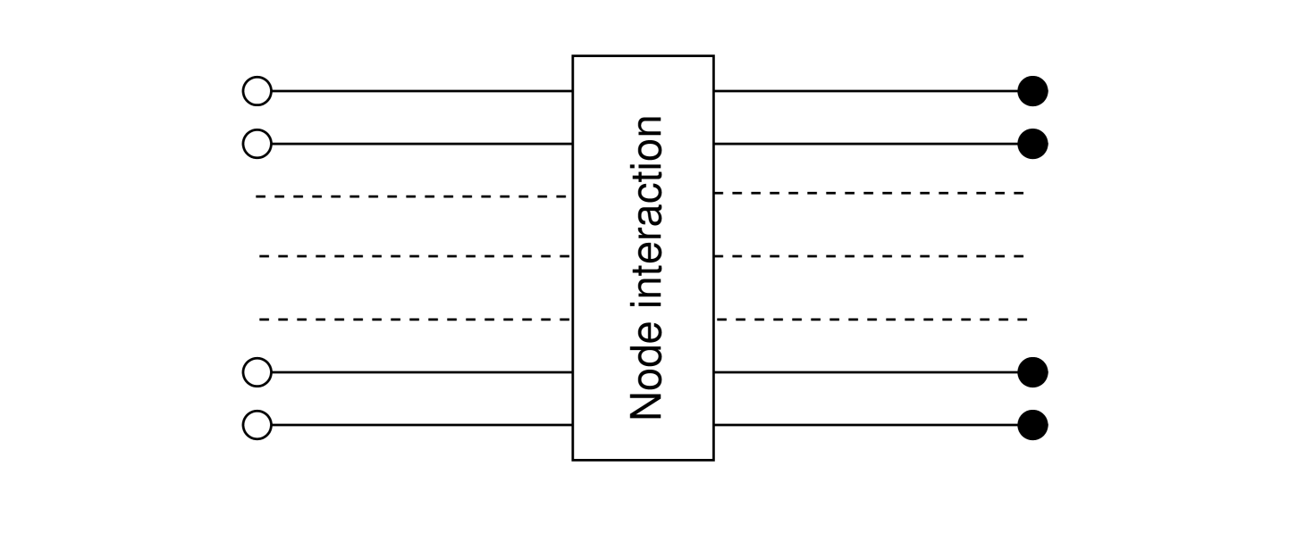
Figure 4: Dynamical/functional module

The initialization sets are represented by the symbols $\circ$, termination sets by $\bullet$. Interaction between nodes occurs only in the event region denoted by the rectangle. Outside of the event region, nodes evolve independently. More generally, we can allow for different number of inputs and outputs: nodes may merge or split.

Our immediate aim is describe some basic operations that we can define on functional asynchronous networks that allow us enable us to find a (maximal) decomposition of a functional asynchronous network into the form shown in figure 3.

V.3 Operations on functional asynchronous networks

If $\mathbf{N}^{a}=(\mathfrak{N}^{a},\mathbb{I}^{a},\mathbb{F}^{a})$, $a\in\mathbf{q}$, are functional asynchronous networks with distinct node sets ($\mathcal{N}^{a}\cap\mathcal{N}^{b}\subset\{N_{0}\}$, $a\neq b\in\mathbf{q}$), define the product $\prod_{a\in\mathbf{q}}\mathbf{N}^{a}$ to be the functional asynchronous network $\mathbf{N}=(\mathfrak{N},\mathbb{I},\mathbb{F})$, where

$$\mathbb{I}=\prod_{a\in\mathbf{q}}\mathbb{I}^{a},\quad\mathbb{F}=\prod_{a\in\mathbf{q}}\mathbb{F}^{a}$$

and $\mathfrak{N}=\prod_{a\in\mathbf{q}}\mathfrak{N}^{a}$ is defined in the obvious way to be the asynchronous network with node set $\mathcal{N}=\cup_{a\in\mathbf{q}}\mathcal{N}^{a}$ (we refer to (BF1, , §6) for details).

We say the $k$-node functional asynchronous network $\mathbf{N}=(\mathfrak{N},\mathbb{I},\mathbb{F})$ is trivial if $\mathbf{N}=\prod_{a\in\mathbf{k}}\mathbf{N}^{a}$ where each $\mathbf{N}^{a}$ has exactly one node $N_{a}$. In particular, if $\mathbf{N}$ is trivial there are no interactions between nodes and no constraints.

Next let $\mathfrak{N}^{a}=(\mathfrak{N}^{a},\mathbb{I},\mathbb{F})$, $a\in\mathbf{q}$, be a family of functional asynchronous networks with common initialization set, termination set and node set $\mathcal{N}=\{N_{0},N_{1},\ldots,N_{k}\}$. Suppose that for each $a\in\mathbf{q}$, there exists $\Sigma(a)\subset\mathbf{k}$ such that

1. $\mathfrak{N}^{a}=\mathfrak{N}^{a}_{1}\times\mathfrak{N}^{a}_{2}$ where $\mathfrak{N}^{a}_{1}$ has node set $\Sigma(a)$ and $\mathfrak{N}^{a}_{2}$ is trivial.

2. If $a\neq b$, $\Sigma(a)\cap\Sigma(b)=\emptyset$.

We define the amalgamation $\mathfrak{N}=\sqcup_{a\in\mathbf{q}}\mathfrak{N}^{a}$ to be the functional asynchronous network $(\prod_{a\in\mathbf{q}}\mathfrak{N}^{a}_{1})\times\mathfrak{N}_{2}$, where $\mathfrak{N}_{2}$ is the trivial network defined as the product of the common trivial factors in $\mathfrak{N}^{a}_{2}$, $a\in\mathbf{q}$. Thus the node set of $\mathfrak{N}_{2}$ will be $\mathbf{k}\smallsetminus\cup_{a\in\mathbf{q}}\Sigma(a)$.

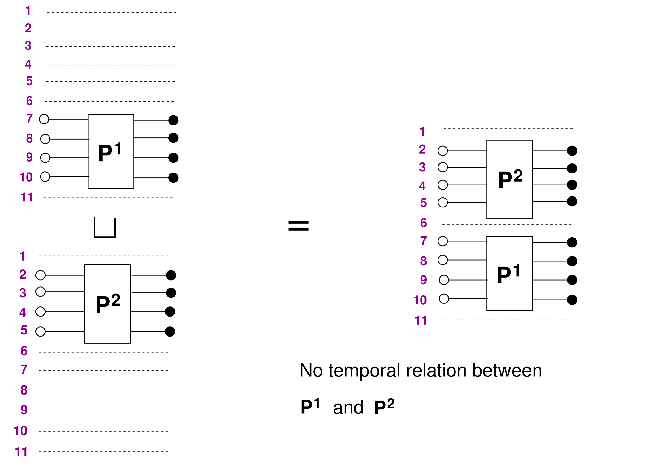
Figure 5: Amalgamating two functional asynchronous networks.

Referring to figure 5, we have $\Sigma(1)=\{7,8,9,10\}$ and $\Sigma(2)=\{2,3,4,5\}$. The amalgamation $\mathbf{P}=\mathbf{P}^{1}\sqcup\mathbf{P}^{2}$ is trivial when restricted to nodes $\{N_{1},N_{6},N_{11}\}$.

Finally, we outline the operation of concatenation, referring the reader to (BF2, , §4) for the details (most) we omit. Suppose that $\mathfrak{N}^{a}=(\mathfrak{N}^{a},\mathbb{I}^{a},\mathbb{F}^{a})$, $a\in\mathbf{2}$, are functional asynchronous networks with common node set. Assume that $\mathbb{F}^{1}=\mathbb{I}^{2}$. The concatenation $\mathbf{N}=(\mathfrak{N},\mathbb{I},\mathbb{F})=\mathbf{N}^{2}\diamond\mathbf{N}^{1}$ will be a temporal merging $\mathbf{N}^{1},\mathbf{N}^{2}$. We define

1. $\mathbb{I}=\mathbb{I}^{1}$, $\mathbb{F}=\mathbb{F}^{2}$.

2. $\mathcal{A}=\{\alpha_{1}\vee\alpha_{2}\mbox{$\;|\;$}\exists\mathbf{X}\in\mathbf{M},\alpha_{1}=\mathcal{E}^{1}(\mathbf{X}),\alpha_{2}=\mathcal{E}^{2}(\mathbf{X})\}$,

where $\vee$ denote the join of the graphs. The definition of the set of admissible vector fields $\mathcal{F}$ for $\mathfrak{N}$ is trickier and requires additional conditions on $\mathbf{N}^{1},\mathbf{N}^{2}$ – we refer to  BF2 for details. We define the event map by $\mathcal{E}(\mathbf{X})=\mathcal{E}^{1}(\mathbf{X})\vee\mathcal{E}^{2}(\mathbf{X}),\mathbf{X}\in\mathbf{M}$. We refer to figure 6 for the operation of concatenation.

Figure 6: Concatenating two functional asynchronous networks.

The concatenation $\mathbf{N}^{2}\diamond\mathbf{N}^{1}$ has the important property that if $\mathbf{N}^{a}$ has generalized transition and timing functions $G^{a}:\mathbb{I}^{a}\times\mbox{$\mathbb{R}$}_{+}^{k}\mbox{$\rightarrow$}\mathbb{F}^{a}$, $\widehat{\mathbf{S}}^{a}:\mathbb{I}^{a}\times\mbox{$\mathbb{R}$}_{+}^{k}\mbox{$\rightarrow$}\mbox{$\mathbb{R}$}_{+}^{k}$, $a\in\mathbf{2}$, then $\mathbf{N}^{2}\diamond\mathbf{N}^{1}$ has generalized transition function $G$ given by $G(\mathbf{X},\mathbf{T})=G^{2}(G^{1}(\mathbf{X},\mathbf{T}),\widehat{\mathbf{S}}^{1}(\mathbf{X},\mathbf{T}))$ (BF2, , Corollary 4.15).

Remark 3.

We have deliberately avoided listing the detailed properties required of functional asynchronous networks in order to define amalgamations and concatenations. Briefly, apart from requiring the existence of generalized transition and timing functions, we require (1) the uncoupled vector vectors defining intrinsic dynamics of a node $N_{i}$ to be transverse to $\mathbb{I}_{i}$, $\mathbb{F}_{i}$ and (2) a local product structure on the network. We refer to (BF2, , §3) for the details.

VI Modularization of dynamics and function

A functional asynchronous network is primitive if it cannot be written as a nontrivial amalgamation or concatenation.

Theorem 1.

Under general conditions, a functional asynchronous network $\mathbf{N}$ has a unique (up to rearrangements) decomposition

$$\mathbf{N}=\mathbf{N}^{q}\diamond\ldots\diamond\mathbf{N}^{1},$$

where $\mathbf{N}^{j}=\mathbf{N}^{j,1}\sqcup\ldots\sqcup\mathbf{N}^{j,q(j)}$, $j\in\mathbf{q}$, and and each $\mathbf{N}^{j,\ell}$ is primitive.

The generalized transition function $G$ for $\mathbf{N}$ can be expressed in terms of the generalized transition and timing functions $G^{j},\widehat{\mathbf{S}}_{j}$ of $\mathbf{N}^{j}$ (or $G^{j,\ell}$ for $\mathbf{N}^{j,\ell}$) by:

$$G(\mathbf{X},\mathbf{T}) = G^{q}(\ldots G^{2}(G^{1}(\mathbf{X},\mathbf{T}),\widehat{\mathbf{S}}^{1}(\mathbf{X},\mathbf{T}))\ldots),$$

$$\widehat{\mathbf{S}}(\mathbf{X},\mathbf{T}) = \widehat{\mathbf{S}}^{q}(\ldots\widehat{\mathbf{S}}^{2}(G^{1}(\mathbf{X},\mathbf{T}),\widehat{\mathbf{S}}^{1}(\mathbf{X},\mathbf{T}))\ldots),$$

$$G^{j} = G^{j,1}\times\ldots\times G^{j,q(j)},\;j\in\mathbf{q}.$$

Example 2.

Consider the network shown in figure 3 and assume that each event $\mathbf{P}^{j}$. $j\in\{a,\ldots,h\}$ is primitive. A decomposition satisfying the requirements of theorem 1 is indicated in figure 7 – the dashed lines indicate the initialization and termination sets for the subnetworks.

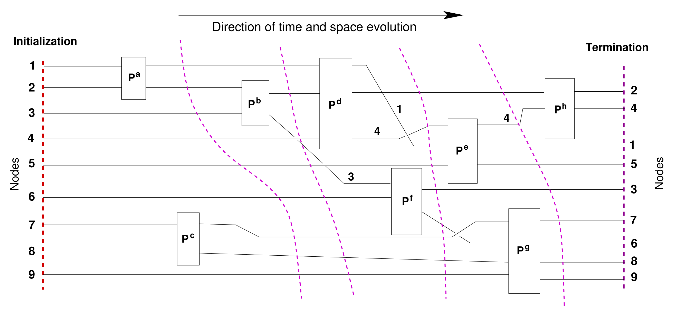
Figure 7: Factorization of network of figure 3.

The factorization for the network is

$$\mathbf{N}=\mathbf{P}^{h}\diamond(\mathbf{P}^{e}\sqcup\mathbf{P}^{g})\diamond(\mathbf{P}^{d}\sqcup\mathbf{P}^{f})\diamond\mathbf{P}^{b}\diamond(\mathbf{P}^{a}\sqcup\mathbf{P}^{c}).$$

This factorization corresponds to maximizing from the left hand side. However, if we maximize from the right we obtain the factorization

$$\mathbf{N}=(\mathbf{P}^{h}\sqcup\mathbf{P}^{g})\diamond(\mathbf{P}^{c}\sqcup\mathbf{P}^{e}\sqcup\mathbf{P}^{f})\diamond\mathbf{P}^{d}\diamond\mathbf{P}^{b}\diamond\mathbf{P}^{a}.$$

In either case there is a concatenation of five networks – that is the minimum number possible.

Theorem 1 allows us to write the function of a network explicitly in terms of the transition functions of the constituent subnetworks.

Results of this type depend crucially on intermittent connection structure and nonsmooth dynamics. For example, no such result is possible for a classical coupled network of phase oscillators.

The approach works because we have adopted an engineer’s viewpoint: we emphasise function rather than dynamics. Indeed, we are indifferent to the specific dynamics occurring between the initialization and termination sets. Of course, both the timing and transition functions provide the key information about network function.

VII Concluding comments

1. Theorem 1 is a prototypical theorem providing proof of concept. The conditions for the theorem can be significantly weakened from those required in BF2 .

2. The theorem yields maximal feedforward structure on a functional asynchronous network (note that individual events may have feedback loops).

3. The result suggests the utility of starting with a small functional asynchronous network; understanding the structure in depth and then then evolving to optimize function (for example by adding feedback).

4. There are many as yet unexplored issues such as bifurcation, hidden deadlocks, and the effects of noise.

5. There is the problem of how far one can determine internal structure on the basis of input/output time series data.

References

- (1) U Alon. An Introduction to Systems Biology. Design Principles of Biological Circuits (Chapman & Hall/CRC, Boca Raton, 2007).
- (2) M di Bernardo, C J Budd, A R Champneys, & P Kowalczyk. Piecewise-smooth Dynamical Systems (Springer, Applied Mathematical Science 163, London, 2008).
- (3) C Bick & M J Field. ‘Asynchronous networks and event driven dynamics’, (2016), preprint.
- (4) C Bick & M J Field. ‘Asynchronous networks: Modularization of Dynamics Theorem’, (2016), preprint.
- (5) N Caporale & Y Dan. ‘Spike timing dependent plasticity: a Hebbian learning rule’ Annu. Rev. Neurosci. 31 (2008), 25–36.
- (6) A F Filippov. Differential Equations with Discontinuous Righthand Sides (Kluwer Academic Publishers, 1988).
- (7) W Gerstner, R Kempter, L J van Hemmen & H Wagner. ‘A neuronal learning rule for sub-millisecond temporal coding’, Nature 383 (1996), 76–78.
- (8) W Gerstner & W Kistler. Spiking Neuron Models (Cambridge University Press, 2002).
- (9) N Kashtan & U Alon. ‘Spontaneous evolution of modularity and network motifs’, PNAS 102 (39) (2005), 13773–13778.
- (10) J Ladyman, J Lambert, and K Wiesner. ‘What is a complex system?’, Eur. J. for Phil. of Sc. 3(1) (2013), 33–67.
- (11) A Morrison, M Diesmann & W Gerstner. ‘Phenomenological models of synaptic plasticity based on spike timing’, Biol. Cyber. 98 (2008), 459–478.