On transfer operators on the circle with trigonometric weights

Abstract.

We study spectral properties of the transfer operators $L$ defined on the circle $\mathbb{T}=\mathbb{R}/\mathbb{Z}$ by

$$(Lu)(t)=\frac{1}{d}\sum_{i=0}^{d-1}f\left(\frac{t+i}{d}\right)u\left(\frac{t+i}{d}\right),\ t\in\mathbb{T}$$

where $u$ is a function on $\mathbb{T}$. We focus in particular on the cases $f(t)=|\cos(\pi t)|^{q}$ and $f(t)=|\sin(\pi t)|^{q}$, which are closely related to some classical Fourier-analytic questions. We also obtain some explicit computations, particularly in the case $d=2$. Our study extends work of Strichartz [10] and Fan and Lau [3].

1. Introduction

Let $\mathbb{T}=\mathbb{R}/\mathbb{Z}$ and identify it with $[0,1]$ in the usual way. For integers $d\geq 2$, let $F$ be the $d$-adic Bernoulli map

$$F:\mathbb{T}\rightarrow\mathbb{T},\ t\mapsto d\cdot t\mod 1.$$

Let $f$ be a function (weight) on $\mathbb{T}$. Consider the weighted transfer operator $L$ associated to $F$:

$$(Lu)(t) =\frac{1}{d}\sum_{s\in F^{-1}(t)}f(s)u(s)$$

$$=\frac{1}{d}\sum_{i=0}^{d-1}f\left(\frac{t+i}{d}\right)u\left(\frac{t+i}{d}\right),\ t\in\mathbb{T}$$

where $u$ is a function on $\mathbb{T}$. Such operators are also called Ruelle (or Ruelle-Perron-Frobenius) operators. They can also be defined associated to more general maps and on more general spaces (cf. Hennion [5] and Baladi [2] for more background).

In this paper, we study spectral properties of $L$ as an operator acting on $C(\mathbb{T})$, the space of continuous functions on $\mathbb{T}$. When $f\equiv 1$, this question has been extensively studied, especially in the case $d=2$ (cf. Vepštas [11] and references therein). For more general weights $f$, there are Perron-Frobenius type theorems that describe spectral properties of $L$ (cf. [2, Theorem 1.5]). However, such theorems often require $f$ to be strictly positive, which is not met by the main examples we are interested in:

$$(c)\ f(t)=|\cos(\pi t)|^{q}\hskip 28.45274pt(s)\ f(t)=|\sin(\pi t)|^{q}$$

where $q>0$. In Section 2, we develop Perron-Frobenius type theorems for transfer operators $L$ with such ‘degenerate’ weights (more precisely, weights that have exactly one zero on $\mathbb{T}$). The theorems are derived using notions of quasicompactness and Krein property, which we verify by exploiting the specific structure of the Bernoulli map $F$; see also Fan and Lau [3] for similar treatments. As a corollary, we conclude that the operator $L$ satisfies classical Perron-Frobenius theorems in all cases of $d$ and $(c)/(s)$, except for the case $d=2$ and $(c)$.

In Section 3, we study in more detail the spectral properties of $L$ in the non-exceptional cases. When $q$ is an even integer, we obtain explicit computations of $\rho(L)$ (the spectral radius of $L$) by reducing to a finite-dimensional problem. When $q$ is not an even integer, evaluating $\rho(L)$ is more difficult. We derive in this case estimations of $\rho(L)$, particularly for $d=3$ (note that when $d$ is odd, $(c)$ and $(s)$ are equivalent). As an application, we obtain asymptotic behavior of some integrals of the form

$$I_{n}=\int_{\mathbb{T}}\prod_{j=0}^{n-1}f(d^{j}t)dt,\quad\text{as }n\rightarrow\infty.$$

In particular, we extend a result of Strichartz [10] concerning the Fourier transform of the middle-third Cantor set. We also study geometric properties of the function $L1$, as well as asymptotic behavior of $\rho(L)$ as $q\rightarrow\infty$. For the latter question it turns out that one needs to distinguish the case when $d$ is even and $f$ is given by $(s)$.

In Section 4, we give a detailed account of the exceptional case $d=2$ and $(c)$. Using an explicit formula for the iterates $L^{n}1$, we find the spectral radius and eigenfunctions of $L$ explicitly (see also Fan and Lau [3] for related results), and obtain geometric properties of $L^{n}1$ for $n\geq 1$ (especially for $q\leq 1$ and even $q$’s). The spectral problem in this case is closely related to the case $f\equiv 1$ mentioned above, and has to do with the Hurwitz zeta functions.

In Section 5, we study the spectral problem on Lebesgue spaces. In Section 6, we give an application to Fourier multipliers.

2. Quasicompact transfer operators

Let $f:\mathbb{R}\to\mathbb{R}$ be a continuous nonnegative 1-periodic function, and let $d\geq 2$ be an integer. We consider the transfer operator

(1) $$(Lu)(t)=\frac{1}{d}\sum_{i=0}^{d-1}f\left(\frac{t+i}{d}\right)u\left(\frac{t+i}{d}\right).$$

Let $\mathbb{T}=[0,1]$ with $0$ and $1$ identified (circle). Let $C(\mathbb{T})$ be the Banach space of continuous complex-valued functions on $\mathbb{T}$ endowed with the maximum norm $\|\cdot\|_{\infty}$. Then $L:C(\mathbb{T})\to C(\mathbb{T})$ is a bounded linear operator. Moreover, $L$ is positive in the sense that $u\geq 0$ implies $Lu\geq 0$.

Define a map $F:\mathbb{T}\to\mathbb{T}$ by $F(t)=d\cdot t\mod 1$. Then we can write

$$(Lu)(t)=\frac{1}{d}\sum_{s\in F^{-1}(t)}f(s)u(s),\quad t\in\mathbb{T}.$$

For each $n\in\mathbb{N}$, set

$$f_{n}(t)=\prod_{j=0}^{n-1}f\big{(}F^{j}(t)\big{)}.$$

Then

(2) $$(L^{n}u)(t)=\frac{1}{d^{n}}\sum_{s\in F^{-n}(t)}f_{n}(s)u(s).$$

Let $0<\alpha\leq 1$. Consider the Banach space $C^{\alpha}(\mathbb{T})$ of Hölder continuous functions $u:\mathbb{T}\to\mathbb{C}$ with the norm

$$\|u\|_{\alpha}=\sup_{s\neq t}\frac{|u(s)-u(t)|}{|s-t|^{\alpha}}+\|u\|_{\infty}.$$

If $f\in C^{\alpha}(\mathbb{T})$ then $L_{\alpha}u=Lu$ defines a bounded linear operator $L_{\alpha}:C^{\alpha}(\mathbb{T})\to C^{\alpha}(\mathbb{T})$.

Let $T$ be a bounded linear operator on a Banach space $X$. We denote its spectral radius by $\rho(T)$. $T$ is called quasicompact if there exists a compact operator $K$ on $X$ such that $\rho(T-K)<\rho(T)$. If $T$ is quasicompact and $\lambda\in\mathbb{C}$ is in the spectrum of $T$ with $|\lambda|>\rho(T-K)$, then $\lambda$ is an eigenvalue of $T$.

The following theorem is proved in [9, pages 3–4]. In [9, Proposition 1] it is assumed that $f$ is positive while we assume here that $f$ is nonnegative. However positivity of $f$ is not used on pages 3–4 of [9]. See also [5].

Theorem 2.1.

Let $0\leq f\in C^{\alpha}(\mathbb{T})$ for some $0<\alpha\leq 1$. Then $\rho(L)=\rho(L_{\alpha})$. Furthermore, if $\rho(L)>0$, then $L_{\alpha}$ is quasicompact.

For each $n\in\mathbb{N}$, set

(3) $$h_{n}=L^{n}1.$$

Define

(4) $$r_{n}=\min_{t\in\mathbb{T}}h_{n}(t),\quad R_{n}=\max_{t\in\mathbb{T}}h_{n}(t).$$

It is easy to show that

$$r_{m+n}\geq r_{m}r_{n},\quad R_{m+n}\leq R_{m}R_{n}.$$

Therefore, the limits

(5) $$r=\lim_{n\to\infty}(r_{n})^{1/n}=\sup_{n}\ (r_{n})^{1/n},\quad R=\lim_{n\to\infty}(R_{n})^{1/n}=\inf_{n}\ (R_{n})^{1/n}$$

exist. In particular, for every $n\in\mathbb{N}$ we have

(6) $$r_{n}^{1/n}\leq r\leq R\leq R_{n}^{1/n}.$$

Moreover, since $R_{n}=\|L^{n}\|_{C(\mathbb{T})\rightarrow C(\mathbb{T})}$, by Gelfand’s formula, $R=\rho(L)$.

Theorem 2.2.

Let $w\in C(\mathbb{T})$ be a unit, that is, $w(t)>0$ for all $t\in\mathbb{T}$. Then

(7) $$\min_{t\in\mathbb{T}}\frac{(Lw)(t)}{w(t)}\leq r\leq R\leq\max_{t\in\mathbb{T}}\frac{(Lw)(t)}{w(t)}.$$

Proof.

We define a bounded linear operator $S$ on $C(\mathbb{T})$ by

$$(Su)(t)=\frac{1}{w(t)}L(wu)(t),$$

a sequence of functions

$$\tilde{h}_{n}=S^{n}1,$$

and sequences of numbers

$$\tilde{r}_{n}=\min_{t\in\mathbb{T}}\tilde{h}_{n}(t),\quad\tilde{R}_{n}=\max_{t\in\mathbb{T}}\tilde{h}_{n}(t).$$

Since $S$ is positive, we obtain for every $n\in\mathbb{N}$

$$(\tilde{r}_{n})^{1/n}\leq\lim_{n\to\infty}(\tilde{r}_{n})^{1/n}=:\tilde{r}\leq\tilde{R}:=\lim_{n\to\infty}(\tilde{R}_{n})^{1/n}\leq(\tilde{R}_{n})^{1/n}.$$

Since $w$ is a unite, there are constants $a,b>0$ such that

$$a\leq w(t)\leq b$$

for all $t\in\mathbb{T}$. This implies

$$ah_{n}(t)=(L^{n}a)(t)\leq w(t)\tilde{h}_{n}(t)\leq(L^{n}b)(t)=bh_{n}(t).$$

From this we obtain

$$r_{n}\leq\frac{b}{a}\tilde{r}_{n},\quad\tilde{r}_{n}\leq\frac{b}{a}r_{n},\quad R_{n}\leq\frac{b}{a}\tilde{R}_{n},\quad\tilde{R}_{n}\leq\frac{b}{a}R_{n}.$$

Thus

$$r=\tilde{r},\quad R=\tilde{R}.$$

Now (7) follows from

$$\tilde{r}_{1}\leq\tilde{r}=r\leq\tilde{R}=R\leq\tilde{R}_{1}.$$

∎

We say that $L$ is a Krein operator if, for all $u\in C(\mathbb{T})$ such that $u(t)\geq 0$ for all $t\in\mathbb{T}$ but $u(t_{0})>0$ for at least one $t_{0}\in\mathbb{T}$, there is $n\in\mathbb{N}$ such that $L^{n}u$ is a unit. Note that $n$ may depend on $u$. It is easy to show that a Krein operator carries units to units (cf. [1, Lemma 5.2]). It follows from (2) that if $f(t)>0$ for all $t$ then $L$ is a Krein operator, Also, if $f$ vanishes on an interval of positive length, then $L$ cannot be a Krein operator.

Lemma 2.3.

Suppose $f$ has exactly one zero in $[0,1)$. If $f_{n}$ has four zeros that form an arithmetic progression with step size $d^{-n}$, then $d=2$ and $f(\frac{1}{2})=0$.

Proof.

Let $s_{0}+\mathbb{Z}$ be the set of zeros of $f$. Suppose that $t_{i}=t+id^{-n}$ is a zero of $f_{n}$ for $i=0,1,2,3$. Then there exist integers $0\leq k_{i}\leq n-1$, and integers $j_{i}$ such that

(8) $$t_{i}=d^{-k_{i}}(s_{0}+j_{i}),\quad i=0,1,2,3.$$

We will assume that $k_{0}=\max\{k_{0},k_{1},k_{2},k_{3}\}$ (the other cases are mentioned at the end of the proof.) Clearly, $k_{0}>k_{1}$. Since we can replace $s_{0}$ by $s_{0}+j$ with any integer $j$, we will assume that $j_{1}=0$ in order to simplify the notation. From $t_{1}-t_{0}=t_{2}-t_{1}=d^{-n}$, we obtain

$$d^{-k_{1}}s_{0}-d^{-k_{0}}(s_{0}+j_{0})=d^{-n},\quad d^{-k_{2}}(s_{0}+j_{2})-d^{-k_{1}}s_{0}=d^{-n}.$$

Eliminating $s_{0}$ from these equations, we find

$$(1-j_{0}d^{n-k_{0}})(d^{k_{0}-k_{1}}-d^{k_{0}-k_{2}})=(1-j_{2}d^{n-k_{2}})(1-d^{k_{0}-k_{1}}).$$

This is an equation involving only integers. Since $n>k_{2}$, $k_{0}>k_{1}$, the right-hand side is not divisible by $d$. Therefore, we must have $k_{0}=k_{2}$. But this is impossible when $d>2$. So we must have $d=2$ and $k_{0}=k_{2}=n-1$.

Now suppose that $d=2$ and $k_{0}=k_{2}=n-1$. Without loss of generality we take $j_{0}=0$, $j_{2}=1$. Since $t_{1}-t_{0}=t_{3}-t_{2}=2^{-n}$ we obtain

$$2^{n-k_{1}}(s_{0}+j_{1})=2s_{0}+1,\quad 2^{n-k_{3}}(s_{0}+j_{3})=2s_{0}+3.$$

Eliminating $s_{0}$ this gives

$$(3-j_{3}2^{n-k_{3}})(2^{n-k_{1}-1}-1)=(1-j_{1}2^{n-k_{1}})(2^{n-k_{3}-1}-1).$$

It is clear that $k_{1}<n-1$, $k_{3}<n-1$. Therefore, the equation yields that $2^{n-k_{3}-2}-3\cdot 2^{n-k_{1}-2}+1$ is an even integer. This implies that $k_{1}=n-2$ or $k_{3}=n-2$. If $k_{1}=n-2$ then $2s_{0}+1=4(s_{0}+j_{1})$, which implies that $s_{0}-\frac{1}{2}$ is an integer. If $k_{3}=n-2$, we have the same conclusion.

If $k_{2}=\max\{k_{0},k_{1},k_{2},k_{3}\}$, the proof is almost the same. We again obtain $k_{0}=k_{2}=n-1$ and $d=2$ after the first part of the proof. The other two cases can be reduced to the treated ones by replacing $s_{0}$ by $-s_{0}$. ∎

Lemma 2.4.

Suppose $f$ has exactly one zero $s_{0}\in[0,1)$. Then $L$ is a Krein operator unless $s_{0}=\frac{1}{2}$ and $d=2$.

Proof.

Let $u\in C(\mathbb{T})$ be nonnegative but not identically zero, Choose $n$ so large that $u(t)>0$ for $md^{-n}\leq t\leq(m+4)d^{-n}$ for some integer $m$, $0\leq m\leq d^{n}-4$. We claim that $(L^{n}u)(t)>0$ for all $t\in\mathbb{T}$. In fact, by Lemma 2.3, if $t\in\mathbb{T}$ then among the four points $t_{i}=d^{-n}(t+m+i)$, $i=0,1,2,3$, at least one satisfies $f_{n}(t_{i})>0$. Then (2) implies $(L^{n}u)(t)\geq f_{n}(t_{i})u(t_{i})>0$. ∎

If $d=2$ and $f(\frac{1}{2})=0$ then $L$ is not a Krein operator: If $u(0)=0$ then $(L^{n}u)(0)=0$ for all $n\in\mathbb{N}$.

Theorem 2.5 (See also [3]).

Suppose that $L$ is a Krein operator. Then the following statements hold.
(a) $R>0$.
(b) If $Lv=\lambda v$ with $v\neq 0$ and $|\lambda|=R$, then there is a constant $\theta\in\mathbb{R}$ such that $e^{-i\theta}v$ is a unit.
(c) $L$ has no eigenvalue $\lambda$ on the circle $|\lambda|=R$ except possibly $\lambda=R$.
(d) If $R$ is an eigenvalue of $L$, then its algebraic multiplicity is $1$.
(e) If $0\leq f\in C^{\alpha}(\mathbb{T})$, then $L_{\alpha}$ is quasicompact, $r=R$, and $R$ is an eigenvalue of $L_{\alpha}$ of algebraic multiplicity $1$ with a unit eigenfunction.

Proof.

(a) Since $L$ is a Krein operator, $h_{1}=L1$ is a unit, so $0<r_{1}\leq R$.

(b) $Lv=\lambda v$ implies $z:=L|v|-R|v|\geq 0$. Suppose that $z$ is not identically zero. Then there is $n\in\mathbb{N}$ such that $L^{n}z$ and $w:=L^{n}|v|$ are units. It follows that there is $\delta>0$ such that

$$(L^{n}z)(t)=(Lw)(t)-Rw(t)\geq\delta w(t),\quad t\in\mathbb{T}.$$

Applying Theorem 2.2, we obtain the contradiction

$$R+\delta\leq\min_{t\in\mathbb{T}}\frac{(Lw)(t)}{w(t)}\leq R.$$

Therefore, $z=0$ and

(9) $$L|v|=R|v|.$$

Then

$$|L^{n}v|=R^{n}|v|=L^{n}|v|=w.$$

Therefore, $|v|$ is a unit. We claim that there is a constant $\theta\in\mathbb{R}$ such that $e^{-i\theta}v(t)>0$ for all $t$. Suppose this is not true. Since $L|v|=|Lv|$, there is $n\in\mathbb{N}$ and $1\leq i<j\leq d^{n}$ such that $v(s)/v(t)\not\in(0,\infty)$ for all $s\in I_{n,i}$, $t\in I_{n,j}$. Since $L$ is a Krein operator, $f$ does no vanish on an interval of positive length. Then also $f_{n}$ does not vanish on an interval of positive length. Therefore, there is $s\in I_{n,i}$, $t\in I_{n,j}$ with $(t-s)d^{-n}\in\mathbb{Z}$ such that $f_{n}(s)\neq 0$, $f_{n}(t)\neq 0$. Hence, by (2), $|(L^{n}v)(s)|<(L^{n}|v|)(s)$, which is a contradiction. Therefore, the claim is proved.

(c) follows from (b).

(d) Suppose that $R$ is an eigenvalue of $L$. By (b), each corresponding eigenfunction is a constant multiple of a unit. It follows that the geometric multiplicity of the eigenvalue $R$ is $1$. Now assume that there are $u,w\in C(\mathbb{T})$ such that $Lu-Ru=w$, $Lw=Rw$, where $w$ is a unit. We may assume that $u$ is a unit. There is $\delta>0$ such that $\delta u\leq w$. Then Theorem 2.2 leads to the contradiction

$$R+\delta\leq\min_{t\in\mathbb{T}}\frac{(Lu)(t)}{u(t)}\leq R.$$

This shows that the algebraic multiplicity of the eigenvalue $R$ is $1$.

(e) Since $\rho(L)=R>0$, it follows from Theorem 2.1 that $L_{\alpha}$ is quasicompact. Then $L_{\alpha}$ has an eigenvalue $\lambda$ on the circle $|\lambda|=R$. By (c), $R$ is an eigenvalue of $L_{\alpha}$. There is a corresponding unit eigenfunction. Now $r=R$ follows from Theorem 2.2. ∎

Theorem 2.6 (See also [3]).

Suppose that $0\leq f\in C^{\alpha}(\mathbb{T})$ and that $L$ is a Krein operator. Let $P$ be the spectral projection onto the eigenspace of $L_{\alpha}$ corresponding to the eigenvalue $R$.
(a) The sequence $R^{-n}L_{\alpha}^{n}$ converges to $P$ as $n\to\infty$ with respect to the operator norm.
(b) The sequence $R^{-n}h_{n}$ converges in $C^{\alpha}(\mathbb{T})$ to an eigenfunction of $L_{\alpha}$ corresponding to the eigenvalue $R$.

Proof.

(a) By Theorem 2.5, $L_{\alpha}$ is quasicompact and the eigenvalue $R$ of $L_{\alpha}$ is an isolated point of its spectrum. Therefore, there exists the spectral projection $P$ onto the one-dimensional root subspace belonging to the eigenvalue $R$. The Banach space $C^{\alpha}(\mathbb{T})$ is a direct sum of the subspaces $PC^{\alpha}(\mathbb{T})$ and $(1-P)C^{\alpha}(\mathbb{T})$. Both subspaces are invariant under $L_{\alpha}$. On $PC^{\alpha}(\mathbb{T})$, $L_{\alpha}$ acts as $R$ times the identity. Set $S:=R^{-1}(1-P)L_{\alpha}$. By Theorem 2.5, the spectral radius of $S$ is less than $1$ so $S^{n}$ converges to $0$ as $n\to\infty$ in the operator norm. We have $R^{-n}L_{\alpha}^{n}=S^{n}+P$ which implies statement (a).

(b) We have $R^{-n}h_{n}=R^{-n}L^{n}_{\alpha}1\to P1$ as $n\to\infty$. Since

$$1\leq R^{-n}R_{n}\leq\|R^{-n}h_{n}\|_{\alpha}\to\|P1\|_{\alpha},$$

we have $P1\neq 0$. ∎

We consider now the following problem that was the original motivation for this paper. Let $f:\mathbb{R}\to\mathbb{C}$ be a bounded measurable and 1-periodic function, and let $d\geq 2$ be an integer. For $n\in\mathbb{N}$, define as before

$$f_{n}(t)=\prod_{j=0}^{n-1}f(d^{j}t).$$

The problem is to find the behavior of the sequence of integrals

$$I_{n}(f)=\int_{0}^{1}f_{n}(t)\,dt$$

as $n\to\infty$. In particular, we want to find $c(f)$ defined by

(10) $$c(f)=\limsup_{n\to\infty}|I_{n}(f)|^{1/n}.$$

The sequence $I_{n}$ is related to the bounded linear operator

(11) $$(Tx)(t)=f(t)x(d\cdot t)$$

which maps $L^{2}(\mathbb{T})$ to itself. Note that

$$f_{n}=T^{n}1$$

and

(12) $$I_{n}(f)=\langle T^{n}1,1\rangle$$

with the inner product $\langle\cdot,\cdot\rangle$ in $L^{2}(\mathbb{T})$. In particular,

$$|I_{n}|\leq\|T^{n}\|$$

and

(13) $$c(f)\leq\lim_{n\to\infty}\|T^{n}\|^{1/n}=\rho(T).$$

We show that $c(f)$ is equal to the spectral radius of a transfer operator under suitable assumptions on $f$. See also [3] for related results.

Theorem 2.7.

Suppose that $0\leq f\in C^{\alpha}(\mathbb{T})$ for some $0<\alpha\leq 1$, and that the transfer operator $L$ defined by (1) is a Krein operator. Then $r=c(f)=R=\rho(L)$, where $r,R$ are defined in (5). Moreover, we can replace $\limsup$ by $\lim$ in definition (10).

Proof.

The adjoint $T^{\ast}$ of $T$ agrees with the operator $L$ when considered as an operator on $L^{2}(\mathbb{T})$. Let $h_{n},r_{n},R_{n}$ be defined by (3), (4). It follows from (12) that

$$I_{n}=\langle 1,h_{n}\rangle=\int_{0}^{1}h_{n}(t)\,dt.$$

Thus

$$r_{n}^{1/n}\leq I_{n}^{1/n}\leq R_{n}^{1/n}.$$

By Theorem 2.5(e), the sequences $r_{n}^{1/n}$ and $R_{n}^{1/n}$ converge to the same limit $r=R$. Therefore, the sequence $I_{n}^{1/n}$ converges and we obtain $r=c(f)=R$. ∎

Using Theorem 2.7 in connection with (6) or Theorem 2.2 we can estimate $c(f)$. We will look at some examples in the next section.

We mention two special classes of functions $f$ for which $c(f)$ can be calculated explicitly.

1) Suppose that $f$ is a step function such that $f(t)=f_{i}={\rm const}$ for $\frac{i-1}{d}\leq t<\frac{i}{d}$, $i=1,\cdots,d$. Then it is easy to show that

$$I_{n}(f)=\left(\int_{0}^{1}f(t)\,dt\right)^{n}.$$

Therefore,

$$c(f)=\left|\int_{0}^{1}f(t)\,dt\right|.$$

If $f$ is any nonnegative bounded measurable $1$-periodic function, we may introduce two step function $g,h$ defined by

$$g(t) = \inf\left\{f(s):\frac{i-1}{d}\leq s<\frac{i}{d}\right\}\quad\text{for $\frac{i-1}{d}\leq t<\frac{i}{d}$},$$

$$h(t) = \sup\left\{f(s):\frac{i-1}{d}\leq s<\frac{i}{d}\right\}\quad\text{for $\frac{i-1}{d}\leq t<\frac{i}{d}$}.$$

Then we obtain the estimate

(14) $$I_{n}(g)\leq I_{n}(f)\leq I_{n}(h)$$

and so

(15) $$\int_{0}^{1}g(t)\,dt\leq c(f)\leq\int_{0}^{1}h(t)\,dt.$$

2) Let $f$ be any bounded measurable $1$-periodic function with Fourier expansion

$$f(t)=\sum_{k\in\mathbb{Z}}a_{k}e^{2\pi ikt}.$$

We represent the operator $T$ by an infinite matrix in the orthonormal basis $\{e^{2\pi ikt}\}_{k\in\mathbb{Z}}$. The matrix of $T$ is

(16) $$\left(a_{k-d\ell}\right)_{k,\ell\in\mathbb{Z}}.$$

In this notation $k$ is the row index and $\ell$ is the column index. If we write

$$f_{n}(t)=\sum_{k\in\mathbb{Z}}a_{k,n}e^{2\pi ikt},$$

then we obtain the coefficients $a_{k,n+1}$ from $a_{k,n}$ by application of $T$, so

$$a_{k,n+1}=\sum_{\ell\in\mathbb{Z}}a_{k-d\ell}\,a_{\ell,n}.$$

Note that $I_{n}=a_{0,n}$.

In particular, suppose that $f(t)$ is a trigonometric polynomial of degree $N$, so

$$f(t)=\sum_{k=-N}^{N}a_{k}e^{2\pi ikt}.$$

We set

$$K:=\left\lfloor\frac{N-1}{d-1}\right\rfloor.$$

Consider the central $2K+1$ by $2K+1$ submatrix $B$ of $T$ consisting of rows $-K\leq k\leq K$ and columns $-K\leq\ell\leq K$. Notice that all entries in the rows $-N\leq k\leq N$ outside the central submatrix vanish. Therefore, we obtain the recursion

$$a_{k,n+1}=\sum_{\ell=-K}^{K}a_{k-d\ell}\,a_{\ell,n}\quad\text{if $-K\leq k\leq K$.}$$

Hence we can calculate $I_{n}=a_{0,n}$ by computing the powers of the matrix $B$. It is clear that

(17) $$c(f)\leq\rho(B)$$

but it is not immediately clear whether we have equality in (17). It depends on how the constant function $1$ is represented in a Jordan basis of $B$ (whether the basis vectors associated with largest eigenvalue of $B$ contribute to the expansion of $1$.)

The situation is clear if the matrix $B$ is nonnegative and primitive ($B^{p}$ is a positive matrix for some $p\in\mathbb{N}$.) Then the spectral radius of $B$ is a simple positive eigenvalue and we can use Theorem 8.5.1 in [6] to show that there is equality in (17). Suppose that $a_{k}>0$ for all $k=-N,-N+1,\cdots,N$. Then all entries in the main diagonal, the subdiagonal and superdiagonal of $B$ are positive. Therefore, $B$ is primitive.

If we have symmetry $a_{-k}=a_{k}$ then we can replace the matrix $B$ by a $K+1$ by $K+1$ matrix $C$ whose entries are

$$c_{i,0}=a_{i},\quad c_{i,j}=a_{i-dj}+a_{i+dj}\quad\text{if $0\leq i\leq K$, $1\leq j\leq K$.}$$

See the next section for examples.

3. The special cases $f(t)=|\cos(\pi t)|^{q}$ and $f(t)=|\sin(\pi t)|^{q}$

In this section we consider the functions

$$f(t)=|\cos(\pi t)|^{q},\quad\tilde{f}(t)=|\sin(\pi t)|^{q}\quad\text{where $q>0$}.$$

We set

$$c(q):=c(f),\quad\tilde{c}(q):=c(\tilde{f}).$$

Obviously, $0\leq c(q),\tilde{c}(q)\leq 1$. Note that $f,\tilde{f}\in C^{\alpha}(\mathbb{T})$ with $\alpha=\min(q,1)$. By Lemma 2.4, $L$ is a Krein operator except when $f(t)=|\cos(\pi t)|^{q}$ and $d=2$. This is an exceptional case that will be considered in the next section. Except for this case we can apply Theorems 2.5 and 2.7.

If $d$ is odd, then $I_{n}(f)=I_{n}(\tilde{f})$, and consequently $c(f)=c(\tilde{f})$. In fact, in this case the transfer operators weighted by $f$ and $\tilde{f}$ are conjugate to each other.

Theorem 3.1.

The functions $c(q)$ and $\tilde{c}(q)$ are convex and nonincreasing in $q>0$. Moreover,

$$\lim_{q\to\infty}c(q)=\frac{1}{d},\quad\lim_{q\to\infty}\tilde{c}(q)=\begin{cases}\frac{1}{d}&\text{if $d$ is odd,}\\ 0&\text{if $d$ is even,}\end{cases}$$

and

$$\lim_{q\to 0^{+}}c(q)=\lim_{q\to 0^{+}}\tilde{c}(q)=1.$$

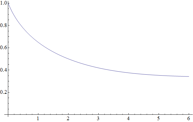
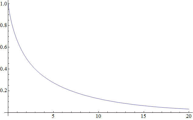
Figure 1. A graph of $c(q)$ for $0<q<6$, when $d=3$.

Figure 2. A graph of $\tilde{c}(q)$ for $0<q<20$, when $d=2$.

Proof.

Monotonicity of $c(q)$ and $\tilde{c}(q)$ are clear. Convexity follows from Hölder’s inequality and Young’s inequality. By looking at the function $h_{1}$ associated with $f$, we see that $R_{1}=\max_{t\in[0,1]}h_{1}(t)$ converges to $d^{-1}$ as $q\to\infty$. So

$$\limsup_{q\to\infty}c(q)\leq d^{-1}.$$

If we use an estimate of the form $f(t)\geq 1-\frac{t}{a}$ for $0\leq t\leq a$ for some $a\in(0,1)$ depending on $q$, then we can estimate

$$f_{n}(t)\geq\prod_{j=0}^{n-1}\left(1-\frac{d^{j}t}{a}\right)\geq\exp\left(-(\ln 4)\,\frac{d^{n}-1}{d-1}\frac{t}{a}\right)\quad\text{for $0\leq t\leq\frac{a}{2d^{n-1}}$}.$$

It then follows from (10) that $c(q)\geq d^{-1}$ for all $q>0$. Hence

$$\lim_{q\to\infty}c(q)=d^{-1}.$$

When treating $\tilde{c}(q)$, we may assume that $d$ is even. The proof is similar to the preceding one. To determine the limit of $\tilde{c}(q)$ as $q\to\infty$, we use $c(\tilde{f})\leq R_{2}^{1/2}$.

To show the limits as $q\to 0^{+}$, it suffices to show that

$$c(q)^{1/q}\geq 1/2,\quad\tilde{c}(q)^{1/q}\geq 1/2$$

for all $q>0$. To this end, let $g(t)=|\cos(\pi t)|$ (or $|\sin(\pi t)|$). By Jensen’s inequality, we have

$$I_{n}^{1/q}=\left(\int_{0}^{1}|g_{n}(t)|^{q}dt\right)^{1/q}\geq\exp\left(\int_{0}^{1}\ln|g_{n}(t)|dt\right)$$

for all $q>0$. On the other hand, since

$$\int_{0}^{1}\ln|\cos(\pi t)|dt=\int_{0}^{1}\ln|\sin(\pi t)|dt=\ln(1/2),$$

we have

$$\int_{0}^{1}\ln|g_{n}(t)|dt=\sum_{j=0}^{n-1}\int_{0}^{1}\ln|g(d^{j}t)|dt=n\ln(1/2).$$

Thus, for any $q>0$,

$$c(q)^{1/q}\ (\text{or }\tilde{c}(q)^{1/q})=\lim_{n\to\infty}I_{n}^{1/(nq)}\geq 1/2.$$

This completes the proof. ∎

3.1. The case $f(t)=\cos^{2N}(\pi t)$, $d=3$

For $N\in\mathbb{N}$, consider the trigonometric polynomial

$$f(t)=\cos^{2N}(\pi t).$$

The degree of $f$ is $N$ and, for $-N\leq k\leq N$,

$$a_{k}=2^{-2N}\binom{2N}{k+N}>0.$$

We use the method 2) from Section 2. If $N=1,2$, then $K=0$ and so $c(2)=\frac{1}{2}$ and $c(4)=\frac{3}{8}$ (note that this recovers a result of Strichartz [10]). If $N=3$, then $K=1$ and

$$C=\frac{1}{64}\left[\begin{array}[]{rr}20&2\\ 15&6\end{array}\right].$$

So

$$c(6)=\rho(C)=\frac{1}{64}(13+\sqrt{79})=0.342003\cdots.$$

If $N=4$, then $K=1$ and

$$C=\frac{1}{256}\left[\begin{array}[]{rr}70&16\\ 56&29\end{array}\right].$$

It follows that

$$c(8)=\rho(C)=\frac{1}{512}(99+9\sqrt{65})=0.335078\cdots.$$

When $N\geq 5$, the formulas for $c(2N)$ become more complicated, but $c(2N)$ is easy to compute numerically. For example, we obtain

$$c(10)=0.333691\cdots.$$

The same method can be used to determine $c(2N)$ for other values of $d$.

3.2. The case $f(t)=|\sin(\pi t)|$, $d=3$

Even if $f$ is not a trigonometric polynomial, we can still use matrix methods to estimate $c(f)$. As an example, consider

(18) $$f(t)=|\sin(\pi t)|.$$

The Fourier coefficients of $f$ are

$$a_{k}=-\frac{2}{\pi}\frac{1}{(2k-1)(2k+1)},\ k\in\mathbb{Z}.$$

Note that $a_{0}>0$ but all other $a_{k}$ are negative. Let $N\in\mathbb{N}$. We estimate

$$f(t)\leq\sum_{k=-N}^{N}a_{k}e^{2\pi ikt}+\frac{2}{\pi}\sum_{k=N+1}^{\infty}\frac{2}{(2k-1)(2k+1)}$$

so we have

$$f(t)\leq h(t),$$

where

$$h(t)=\frac{2}{\pi}\frac{1}{2N+1}+\sum_{k=-N}^{N}a_{k}e^{2\pi ikt}.$$

Using

$$c(f)\leq c(h)\leq\rho(C)$$

we get upper bounds for $c(f)=c(1)$ (when $d=3$):

$N$	$\rho(C)$
1	0.848826
2	0.763943
3	0.737463
4	0.717381
5	0.704696
10	0.678384
20	0.663593
30	0.658613
50	0.654552
100	0.651436

As far as we know the exact value of $c(1)$ is not known. We conjecture that $c(1)=0.648314\cdots$.

We also obtain

$$g(t)\leq f(t)$$

where

$$g(t)=-\frac{2}{\pi}\frac{1}{2N+1}+\sum_{k=-N}^{N}a_{k}e^{2\pi ikt}.$$

Since $a_{0}>0$ and all other $a_{k}<0$, we can easily show that $g(t)\geq 0$. Therefore, we have

$$c(g)\leq c(f).$$

However, the trigonometric polynomial $g$ does not have positive coefficients, so we do not know whether $c(g)=\rho(C)$. Therefore, we do not obtain lower bounds by this method. For $N=100$, one would get $\rho(C)=0.645194\cdots$.

Somewhat surprisingly, the functions $h_{n}$ associated with (18) can be represented in a fairly explicit way. If

$$u(t)=\cos\left(\pi as\right),\quad s=t-\tfrac{1}{2},$$

then

$$(Lu)(t)=\tfrac{1}{6}\big{(}1+2\cos\tfrac{\pi}{3}(1+a)\big{)}\cos\tfrac{\pi}{3}(1+a)s+\tfrac{1}{6}\big{(}1+2\cos\tfrac{\pi}{3}(1-a)\big{)}\cos\tfrac{\pi}{3}(1-a)s.$$

Iterating this formula, we see that $h_{n}$ is a sum of $2^{n-1}$ many terms of the form

$$A\cos(\pi as)$$

where $A>0$ and $a=\frac{1}{3}\pm\frac{1}{9}\pm\frac{1}{27}\pm\cdots\pm\frac{1}{3^{n}}\in(0,\tfrac{1}{2})$. It follows that

$$r_{n}=h_{n}(0),\quad R_{n}=h_{n}(\tfrac{1}{2}).$$

By (5),

$$\left(h_{n}(0)\right)^{1/n}\leq c(f)\leq\left(h_{n}(\tfrac{1}{2})\right)^{1/n}.$$

For example, if $n=1$ we get the bounds

$$\frac{1}{3}\sqrt{3}\leq c(f)\leq\frac{2}{3}.$$

Since $0<a<\frac{1}{2}$, we have

$$R_{n}\leq\sqrt{2}r_{n}.$$

Therefore,

$$(R_{n})^{1/n}\leq 2^{1/(2n)}(r_{n})^{1/n}.$$

In agreement with Theorem 2.7, we get

$$r=R=c(f).$$

We also find that

$$(R_{n})^{1/n}-(r_{n})^{1/n}\leq(R_{n})^{1/n}(1-2^{-1/(2n)})\leq\tfrac{2}{3}(1-2^{-1/(2n)}).$$

For example, if $n=10$, then $c(f)$ is enclosed in the interval $[(r_{n})^{1/n},(R_{n})^{1/n}]$ of length at most $\frac{2}{3}(1-2^{-1/20})=0.0277\cdots$ (the actual length is $0.008390\cdots$.)

By numerical computation, we get the following bounds:

$n$	$(h_{n}(0))^{1/n}$	$(h_{n}(\tfrac{1}{2}))^{1/n}$
1	0.577350	0.666666
2	0.615672	0.656538
3	0.626102	0.653844
4	0.631603	0.652453
5	0.634908	0.651623
10	0.641576	0.649967
15	0.643815	0.649415

3.3. Properties of $h_{n}(t)$ when $f(t)=|\sin(\pi t)|^{q}$

If we use $r_{n}^{1/n}$ and $R_{n}^{1/n}$ to bound $c(f)$, we are faced with the problem to compute the maximum and minimum values of the function $h_{n}$. Therefore, it is of interest to discuss the behavior of the function $h_{n}$. Consider

$$f(t)=|\sin(\pi t)|^{q},\quad d\geq 2.$$

Then we have

$$h_{1}(t)=\frac{1}{d}\sum_{i=0}^{d-1}\left|\sin\Big{(}\pi\frac{t+i}{d}\Big{)}\right|^{q},\quad 0\leq t\leq 1.$$

Note that $h_{1}(t)=h_{1}(1-t)$. For this function we have the following result.

Lemma 3.2.

(a) If $q=2,4,6,\cdots,2(d-1)$, then

$$h_{1}(t)\equiv\frac{1}{2^{q}}\binom{q}{q/2}.$$

(b) Define the intervals

$$Q_{k}=\begin{cases}\big{(}2(k-1),2k\big{)}&\text{if $k=1,\cdots,d-1$,}\\ \big{(}2(d-1),\infty\big{)}&\text{if $k=d$.}\end{cases}$$

Then for $q\in Q_{k}$ we have

$$(-1)^{k-1}h_{1}^{\prime}(t)>0,\quad 0<t<1/2.$$

Proof.

(a) follows from the matrix representation of $T^{\ast}$, the adjoint of the matrix (16).
(b) We differentiate $h_{1}(t)$ to get

(19) $$\frac{d^{2}}{\pi q}h_{1}^{\prime}(t)=\sum_{j=1}^{d}s_{j}^{q}c_{j},\quad 0<t<1,$$

where

$$s_{j}=\sin\left(\pi\frac{t+j-1}{d}\right),\quad c_{j}=\cot\left(\pi\frac{t+j-1}{d}\right).$$

By (a), the left-hand side of (19) is zero for $q=2,4,\cdots,2(d-1)$. Therefore, we obtain a linear system $Vc=b$, where $V$ is a $d\times d$ generalized Vandermonde matrix with entries $s_{j}^{q_{i}}$ in the $i$th row and $j$th column, where $q_{1}=q$ and $q_{i}=2(i-1)$ for $i=2,3,\cdots,d$. The column vector $c$ has components $c_{i}$, and the column vector $b$ has first component $\frac{d^{2}}{\pi q}h_{1}^{\prime}(t)$ and all other components equal to $0$. Suppose that $0<t<\frac{1}{2}$ and $q\in Q_{k}$ for some $k=1,2,\cdots,d$. Then both $s_{1},s_{2},\cdots,s_{d}$ and $q_{1},q_{2},\cdots,q_{d}$ are mutually distinct. It is known (cf.[4, page 76]) that this implies that $\det V\neq 0$, and $\det V>0$ if $s_{1}<s_{2}<\cdots<s_{d}$ and $q_{1}<q_{2}<\cdots<q_{d}$. If we solve the linear system $Vc=b$ for $c$ by Cramer’s rule we find that $c_{1}$ has the same sign as $(-1)^{k-1}h_{1}^{\prime}(t)$. Since $c_{1}>0$, we have $(-1)^{k-1}h_{1}^{\prime}(t)>0$ when $0<t<\frac{1}{2}$ and $q\in Q_{k}$. ∎

Using the bounds $r_{1}\leq c(f)\leq R_{1}$ together with Lemma 3.2, one can deduce for $d=3$

$$\begin{cases}\frac{2}{3}\left(\frac{\sqrt{3}}{2}\right)^{q}\leq c(q)\leq\frac{1}{3}+\frac{2}{3}\left(\frac{1}{2}\right)^{q}&\quad\text{if $0<q\leq 2$ or $q\geq 4$},\\ \frac{1}{3}+\frac{2}{3}\left(\frac{1}{2}\right)^{q}\leq c(q)\leq\frac{2}{3}\left(\frac{\sqrt{3}}{2}\right)^{q}&\quad\text{if $2\leq q\leq 4$}.\end{cases}$$

Note also that Lemma 3.2(a) implies

$$c(q)=\tilde{c}(q)=\frac{1}{2^{q}}\binom{q}{q/2}\quad\text{when }q=2,4,6,\cdots,2(d-1).$$

We would like to extend Lemma 3.2 to $h_{2},h_{3},\cdots$. Based on computer experiments we conjecture the following.

Conjecture 3.3.

Lemma 3.2(b) is true for every $h_{n}$, $n\in\mathbb{N}$.

We obtain sharper lower and upper bounds for $c(f)$ when we choose $w(t)=h_{n}(t)$ in (7). More precisely, we get

(20) $$\min_{t\in[0,1]}\frac{h_{n+1}(t)}{h_{n}(t)}\leq c(f)\leq\max_{t\in[0,1]}\frac{h_{n+1}(t)}{h_{n}(t)}.$$

Here we are faced with the problem to determine the extrema of the quotients $\frac{h_{n+1}(t)}{h_{n}(t)}$. Computer calculations suggest the following.

Conjecture 3.4.

Let $d=3$. If $0<q<2$ and $n$ is odd, then $\frac{h_{n+1}(t)}{h_{n}(t)}$ attains its maximum at $t=0$ and its minimum at $t=\frac{1}{2}$. If $0<q<2$ and $n$ is even, then $\frac{h_{n+1}(t)}{h_{n}(t)}$ attains its maximum at $t=\frac{1}{2}$ and its minimum at $t=0$. If $2<q<4$, then $\frac{h_{n+1}(t)}{h_{n}(t)}$ attains its maximum at $t=0$ and its minimum at $t=\frac{1}{2}$. If $q>4$, then $\frac{h_{n+1}(t)}{h_{n}(t)}$ attains its maximum at $t=\frac{1}{2}$ and its minimum at $t=0$.

If we believe these conjectures then $c(f)$ would lie between $\frac{r_{n+1}}{r_{n}}$ and $\frac{R_{n+1}}{R_{n}}$ for every $n$. In the case $d=3$ we get the following estimates for $c(1)$:

$n$	lower bound	upper bound
1	0.577350	0.666666
2	0.646564	0.656538
3	0.648297	0.648396

We see that these bounds are much better than those from Section 3.2. Unfortunately, we used conjecture 3.4 but for small $n$ it can be proved by direct computation.

4. The case $f(t)=|\cos(\pi t)|^{q}$, $d=2$

In the exceptional case

$$f(t)=|\cos(\pi t)|^{q},\quad d=2$$

we can obtain more explicit computations. See also [3] for related results.

4.1. The integrals $I_{n}$

Using the identity

$$\prod_{j=0}^{n-1}\cos(2^{j}t)=\frac{\sin(2^{n}t)}{2^{n}\sin(t)},$$

we can write

(21) $$f_{n}(t)=\frac{1}{2^{qn}}\frac{|\sin(\pi 2^{n}t)|^{q}}{|\sin(\pi t)|^{q}}.$$

Therefore,

(22) $$I_{n}=\frac{1}{2^{qn}}\int_{0}^{1}\frac{|\sin(\pi 2^{n}t)|^{q}}{|\sin(\pi t)|^{q}}\,dt=\frac{1}{2^{qn-1}}\int_{0}^{1/2}\frac{|\sin(\pi 2^{n}t)|^{q}}{|\sin(\pi t)|^{q}}\,dt.$$

Theorem 4.1.

For $d=2$, we have

$$c(q)=\lim_{n\to\infty}I_{n}^{1/n}=\begin{cases}2^{-q}&\text{if $0<q\leq 1$,}\\ \frac{1}{2}&\text{if $q>1$.}\end{cases}$$

Proof.

Substituting $u=2^{n}t$ in (22), we get

$$I_{n}=\frac{1}{2^{n-1}}\int_{0}^{2^{n-1}}\frac{|\sin(\pi u)|^{q}}{2^{qn}|\sin(\pi 2^{-n}u)|^{q}}\,du.$$

Using

$$\frac{2}{\pi}t\leq\sin t\leq t,\quad 0\leq t\leq\frac{\pi}{2},$$

we find

(23) $$\frac{\pi^{-q}}{2^{n-1}}\int_{0}^{2^{n-1}}\frac{|\sin(\pi u)|^{q}}{u^{q}}\,du\leq I_{n}\leq\frac{2^{-q}}{2^{n-1}}\int_{0}^{2^{n-1}}\frac{|\sin(\pi u)|^{q}}{u^{q}}\,du.$$

If $q>1$, the integral

(24) $$\int_{0}^{\infty}\frac{|\sin(\pi u)|^{q}}{u^{q}}\,du$$

converges. Therefore, the statement of the theorem follows for $q>1$. If $q=1$, the integral (24) diverges and the integrals in (23) behave like $\ln(2^{n})$. Since $n^{1/n}$ converges to $1$ as $n\to\infty$, we obtain the statement of the theorem when $q=1$. If $0<q<1$, the integrals in (23) behave like $2^{n(1-q)}$ which implies the statement of the theorem for $0<q<1$. ∎

4.2. Spectral radius

By (2), we have

$$h_{n}(t)=\frac{1}{2^{n}}\sum_{k=0}^{2^{n}-1}f_{n}\left(\frac{t+k}{2^{n}}\right).$$

Combining with (21), we get

(25) $$h_{n}(t)=\frac{|\sin(\pi t)|^{q}}{2^{n}2^{qn}}\sum_{k=0}^{2^{n}-1}\frac{1}{|\sin(\pi 2^{-n}(t+k))|^{q}}.$$

By estimating the sum in (25) we obtain the following.

Theorem 4.2.

For $f(t)=|\cos(\pi t)|^{q}$, $d=2$, we have

$$r=\frac{1}{2}\quad\text{for all $q>0$}$$

and

$$R=\begin{cases}2^{-q}&\text{if $0<q\leq 1$,}\\ \frac{1}{2}&\text{if $q>1$.}\end{cases}$$

Proof.

Using only the term with $k=0$ in (25), we obtain, for $0\leq t\leq\frac{1}{2}$,

$$h_{n}(t)\geq\frac{1}{2^{n}}\frac{1}{2^{qn}}\frac{|\sin(\pi t)|^{q}}{|\sin(\pi 2^{-n}t)|^{q}}\geq\frac{1}{2^{n}}\frac{2^{q}}{\pi^{q}}.$$

This inequality together with $h_{n}(0)=2^{-n}$ proves $r=\frac{1}{2}$. The proof of the formula for $R$ is elaborated in Section 4.4. ∎

4.3. Eigenfunctions

Let $\alpha=\min\{1,q\}$. By Theorem 2.1, the spectral radii of $L$ and $L_{\alpha}$ agree, and $L_{\alpha}$ is quasicompact. Since $L$ is also a positive operator, $\lambda=R$ must be an eigenvalue, so there must exist a corresponding eigenfunction. But $L$ is not a Krein operator (cf. [1]), so we do not know whether the eigenfunction is unique (up to a constant factor) or whether it is positive on $\mathbb{T}$.

We want to find nontrivial solutions $u\in C(\mathbb{T})$ to the equation $Lu=\lambda u$, particularly for $\lambda=R$. Interestingly, we can find these eigenfunctions fairly explicitly. In fact, if we substitute

$$u(t)=|\sin(\pi t)|^{q}g(t)$$

in $Lu=\lambda u$, we find

(26) $$\tfrac{1}{2}g\left(\tfrac{1}{2}t\right)+\tfrac{1}{2}g\left(\tfrac{1}{2}(t+1)\right)=\mu g(t)\quad\text{where }\mu=2^{q}\lambda.$$

Note that $g(t)$ will usually be continuous only on the open interval $(0,1)$. Much is known about equation (26) (cf. [11]). Clearly, $g(t)=1$ is a solution to (26) with $\mu=1$. Therefore, $u(t)=|\sin(\pi t)|^{q}$ is an eigenfunction of $L$ corresponding to the eigenvalue $\lambda=2^{-q}$. If $0<q\leq 1$, then this is an eigenfunction corresponding to the spectral radius eigenvalue $R$. Furthermore, $g(t)=B_{n}(t)$ with $B_{n}(t)$ denoting a Bernoulli polynomial, is also a solution to (26) corresponding to $\mu=2^{-n}$. This gives us many more eigenfunctions of $L$, but they do not give us eigenfunctions corresponding to the eigenvalue $\lambda=R$ if $q>1$.

Using an idea from [11], we find eigenfunctions corresponding to $\lambda=R$ when $q>1$. For $s>1$, consider the Hurwitz zeta function

(27) $$\zeta(s,t)=\sum_{k=0}^{\infty}\frac{1}{(t+k)^{s}},\quad 0<t<1.$$

It is easy to check that $g(t)=\zeta(s,t)$ is a solution to (26) with $\mu=2^{s-1}$. If we let

(28) $$G(t)=G(s,t):=g(t)+g(1-t),\quad 0<t<1.$$

Then $G(t)$ is also a solution to (26) and has symmetry $G(t)=G(1-t)$. If $s\leq q$, then

$$u(t)=|\sin(\pi t)|^{q}G(t)$$

is a continuous eigenfunction of $L$ corresponding to the eigenvalue $\lambda=2^{s-q-1}$. In particular, choosing $s=q$, we obtain an eigenfunction corresponding to the eigenvalue $R=\frac{1}{2}$.

Suppose $q\geq 2$ is an even integer. Let $s=2,3,\cdots,q$. Consider

$$\widetilde{G}(t)=\zeta(s,t)+(-1)^{s}\zeta(s,1-t)=\sum_{k=-\infty}^{\infty}\frac{1}{(t+k)^{s}}.$$

Since

$$\pi\cot(\pi t)=\lim_{N\to\infty}\sum_{k=-N}^{N}\frac{1}{t+k},$$

we obtain

(29) $$\widetilde{G}(t)=\frac{(-1)^{s-1}\pi}{(s-1)!}\left(\frac{d}{dt}\right)^{s-1}\cot(\pi t),$$

and correspondingly the eigenfunctions

$$u(t)=|\sin(\pi t)|^{q}\widetilde{G}(t).$$

Obviously, these eigenfunctions are trigonometric polynomials. For example, if $q=s=2$, we obtain the eigenfunction

$$u(t)=|\sin(\pi t)|^{2}\widetilde{G}(t)=|\sin(\pi t)|^{2}G(t)=\pi^{2},$$

and, if $q=s=4$, then

(30) $$u(t)=\frac{\pi^{4}}{3}\big{(}\cos(2\pi t)+2\big{)}.$$

We can also find these eigenfunctions in a different way. The space of trigonometric polynomials $\sum_{k=-K}^{K}c_{k}e^{2\pi ikt}$ with $K=(q-2)/2$ is an invariant subspace of $L$. The matrix representation of the restriction of $L$ to this invariant subspace with respect to the basis $\{e^{2\pi ikt}\}$ is

$$B=(a_{2\ell-k})_{-K\leq k,\ell\leq K},$$

where the $a_{k}$ denote the Fourier coefficients in

$$|\cos(\pi t)|^{q}=\sum_{k=-K}^{K}a_{k}e^{2\pi ikt}.$$

For example, if $q=4$ then

$$B=\left[\begin{array}[]{rrr}\frac{1}{4}&\frac{1}{16}&0\\[3.00003pt] \frac{1}{4}&\frac{3}{8}&\frac{1}{4}\\[3.00003pt] 0&\frac{1}{16}&\frac{1}{4}\\ \end{array}\right]$$

This matrix is nonnegative and primitive. Its largest eigenvalue is $\frac{1}{2}$, which follows from the fact that the column sums are all equal to $\frac{1}{2}$. An eigenvector corresponding to the eigenvalue $\lambda=\frac{1}{2}$ is $[1,4,1]^{T}$. Therefore,

$$u(t)=\cos(2\pi t)+2$$

is an eigenfunction of $L$ for $q=4$ corresponding to the eigenvalue $\lambda=\frac{1}{2}$. Apart from a constant factor, this is the same eigenfunction we found in (30). This is true in general. The eigenfunctions of the form $u(t)=|\sin(\pi t)|^{q}\widetilde{G}(t)$ with $\widetilde{G}$ from (29) with $s=2,3,\cdots,q$ match the eigenfunctions obtained from the matrix $B$. In particular, we see that the matrix $B$ has eigenvalues $\frac{1}{2},\frac{1}{4},\cdots,2^{-q+1}$.

In Section 4.5, we study in more detail the trigonometric polynomials obtained from (29).

4.4. Convergence of $h_{n}(t)$

The following proposition shows that, after appropriately normalized, the function $h_{n}$ converges to the eigenfunctions we found in Section 4.3 corresponding to $\lambda=R$.

Proposition 4.3.

The following limits hold in $C^{q}(\mathbb{T})$.
(a) If $0<q<1$, then

$$\lim_{n\rightarrow\infty}2^{qn}h_{n}(t)=\frac{\Gamma(\frac{1}{2}-\frac{q}{2})}{\sqrt{\pi}\Gamma(1-\frac{q}{2})}|\sin(\pi t)|^{q}.$$

(b) If $q=1$, then

$$\lim_{n\rightarrow\infty}\frac{2^{n}}{n}h_{n}(t)=\frac{2\ln 2}{\pi}|\sin(\pi t)|.$$

(c) If $1<q<\infty$, then

$$\lim_{n\rightarrow\infty}2^{n}h_{n}(t)=\pi^{-q}|\sin(\pi t)|^{q}G(q,t).$$

where $G(q,t)$ is given by (28).

Proof.

We show here the pointwise convergence of $h_{n}$. The norm convergence can be shown by slight refinements of the argument.
(a) By (25), we have

$$h_{n}(t)=\frac{|\sin(\pi t)|^{q}}{2^{n}2^{qn}}\sum_{k=0}^{2^{n}-1}\frac{1}{|\sin(\pi 2^{-n}(t+k))|^{q}}.$$

Since

$$\int_{0}^{1}\frac{1}{|\sin(\pi x)|^{q}}dx=\frac{\Gamma(\frac{1}{2}-\frac{q}{2})}{\sqrt{\pi}\Gamma(1-\frac{q}{2})},$$

to prove the statement it suffices to show that

$$\lim_{n\rightarrow\infty}\frac{1}{2^{n}}\sum_{k=0}^{2^{n}-1}\frac{1}{|\sin(\pi 2^{-n}(t+k))|^{q}}=\int_{0}^{1}\frac{1}{|\sin(\pi x)|^{q}}dx.$$

However, this follows easily by treating the left-hand side as a Riemann sum, using the monotonicity of the integrand and the assumption that $q<1$.

(c) Similar as in the proof of (a), we only need to show that

$$\lim_{n\rightarrow\infty}\frac{1}{2^{qn}}\sum_{k=0}^{2^{n}-1}\frac{1}{|\sin(\pi 2^{-n}(t+k))|^{q}}=\pi^{-q}G(q,t).$$

By symmetry, this reduces to showing

$$\lim_{n\rightarrow\infty}\frac{1}{2^{qn}}\sum_{k=0}^{2^{n-1}-1}\frac{1}{|\sin(\pi 2^{-n}(t+k))|^{q}}=\pi^{-q}\sum_{k=0}^{\infty}\frac{1}{(t+k)^{q}}.$$

However, this follows easily from the basic limit

$$\lim_{x\rightarrow 0}\frac{\sin x}{x}=1$$

and the fact that the series on the right-hand side is convergent.

(b) By symmetry, it suffices to show that

$$\lim_{n\rightarrow\infty}\frac{1}{n2^{n}}\sum_{k=0}^{2^{n-1}-1}\frac{1}{\sin(\pi 2^{-n}(t+k))}=\frac{\ln 2}{\pi}.$$

To this end, for any given $\varepsilon>0$ we fix $\delta>0$ such that

$$\left|\frac{x}{\sin x}-1\right|<\varepsilon,\quad 0<x<\delta.$$

We can then write

$$\sum_{k=0}^{2^{n-1}-1}\frac{1}{\sin(\pi 2^{-n}(t+k))}$$

$$= \sum_{k:\,\pi 2^{-n}(t+k)<\delta}\frac{\pi 2^{-n}(t+k)}{\sin(\pi 2^{-n}(t+k))}\frac{1}{\pi 2^{-n}(t+k)}$$

$$+\sum_{k:\,\pi 2^{-n}(t+k)\geq\delta}\frac{1}{\sin(\pi 2^{-n}(t+k))}$$

$$= I+II.$$

By our choice of $\delta$,

$$I =(1+O(\varepsilon))\sum_{k:\,\pi 2^{-n}(t+k)<\delta}\frac{1}{\pi 2^{-n}(t+k)}$$

$$=\frac{2^{n}}{\pi}(1+O(\varepsilon))\sum_{k:\,\pi 2^{-n}(t+k)<\delta}\frac{1}{t+k}$$

$$=\frac{2^{n}}{\pi}(1+O(\varepsilon))(1+o(1))\ln(2^{n})$$

$$=n2^{n}(1+O(\varepsilon))\frac{\ln 2}{\pi},\quad\text{as }n\to\infty.$$

On the other hand, using

$$\sin x\geq\frac{2}{\pi}x,\quad 0\leq x\leq\pi/2,$$

we have

$$II =O(2^{n})\sum_{k:\,\pi 2^{-n}(t+k)\geq\delta}\frac{1}{t+k}$$

$$=O(2^{n})\ln\Big{(}\frac{1}{\delta}\Big{)}$$

$$=o(n2^{n}),\quad\text{as }n\to\infty.$$

Combining these, we get

$$\frac{1}{n2^{n}}(I+II)=(1+O(\varepsilon))\frac{\ln 2}{\pi},\quad\text{as }n\to\infty.$$

Since $\varepsilon$ is arbitrary, this completes the proof. ∎

4.5. Properties of $h_{n}(t)$

It turns out that the functions $h_{n},n\in\mathbb{N}$ share some common geometric properties. We were able to prove some of them.

Proposition 4.4.

(a) If $0<q\leq 1$, then $h_{n}^{\prime\prime}(t)<0$ for all $n\in\mathbb{N}$ and $t\in(0,1)$.
(b) If $1<q<2$, then $h_{n}^{\prime\prime}(1/2)<0$ for $n=1,\cdots,N(q)$, where $N(q)$ satisfies $\lim_{q\rightarrow 1^{+}}N(q)=\infty$.
(c) If $2<q<\infty$, then $h_{n}^{\prime\prime}(1/2)>0$ for $n=1,\cdots,N(q)$, where $N(q)$ satisfies $\lim_{q\rightarrow\infty}N(q)=\infty$.

Proof.

(a) In the case $n=0$, $h_{0}(t)\equiv 1$, so the statement obviously holds with strict inequality replaced by equality. Assume that $h_{n-1}^{\prime\prime}(t)\leq 0$ for all $t\in(0,1)$. We now show that $h_{n}^{\prime\prime}(t)<0$ for all $t\in(0,1)$.

By definition, we have

$$h_{n}(t)=\frac{1}{2}\Big{|}\cos\Big{(}\pi\frac{t}{2}\Big{)}\Big{|}^{q}h_{n-1}\Big{(}\frac{t}{2}\Big{)}+\frac{1}{2}\Big{|}\cos\Big{(}\pi\frac{t+1}{2}\Big{)}\Big{|}^{q}h_{n-1}\Big{(}\frac{t+1}{2}\Big{)}.$$

Since the second term equals the first term after the change of variable $t\rightarrow 1-t$, it suffices to show $(fg)^{\prime\prime}(t)<0$ for all $t\in(0,1/2)$, where

$$f(t)=|\cos(\pi t)|^{q},\quad g(t)=h_{n-1}(t).$$

However, by the product rule,

$$(fg)^{\prime\prime}=f^{\prime\prime}g+2f^{\prime}g^{\prime}+fg^{\prime\prime}.$$

Since $q\leq 1$, we have $f^{\prime\prime}(t)<0$ for all $t\in(0,1/2)$. Also, by symmetry we have $g^{\prime}(1/2)=0$, and so the induction hypothesis implies $g^{\prime}(t)\geq 0$ for all $t\in(0,1/2)$. Combining these we get $f^{\prime\prime}g<0$, $f^{\prime}g^{\prime}\leq 0$, and $fg^{\prime\prime}\leq 0$, which gives $(fg)^{\prime\prime}(t)<0$ for all $t\in(0,1/2)$. This completes the proof by induction.

(b) The proof is similar to that of (a). Using the same notation, we observe that

$$f^{\prime\prime}(t)=\pi^{2}q|\cos(\pi t)|^{q}\Big{(}q|\sin(\pi t)|^{2}-1\Big{)},\quad 0<t<1/2$$

now changes sign at

$$t=t_{q}:=\pi^{-1}\arcsin(\sqrt{1/q}).$$

Notice that $t_{q}>1/4$ if $q<2$, and $t_{q}<1/4$ if $q>2$; moreover,

$$\lim_{q\rightarrow 1^{+}}t_{q}=1/2,\quad\lim_{q\rightarrow\infty}t_{q}=0.$$

In order to determine the sign of

(31) $$(fg)^{\prime\prime}=f^{\prime\prime}g+2f^{\prime}g^{\prime}+fg^{\prime\prime},$$

as before we want all the three terms to have the same sign.

In the case $n=1$, since $g\equiv 1$, we have $(fg)^{\prime\prime}(t)=f^{\prime\prime}(t)<0$ for all $t\in(0,2t_{q})$, where $2t_{q}>1/2$ and $2t_{q}\rightarrow 1$ as $q\rightarrow 1^{+}$. This implies $h_{1}^{\prime\prime}(t)<0$ for all $t\in(1-2t_{q},2t_{q})$. By symmetry we have $h_{1}^{\prime}(t)>0$ for all $t\in(1-2t_{q},1/2)$. Now proceeding by induction, we see that, using (31),

$$h_{n}^{\prime\prime}(t)<0,\quad t\in(2^{n-1}(1-2t_{q}),1-2^{n-1}(1-2t_{q}))$$

and

$$h_{n}^{\prime}(t)>0,\quad t\in(2^{n-1}(1-2t_{q}),1/2).$$

In particular, if $q>1$ is sufficiently close to 1, we have $2^{n-1}(1-2t_{q})<1/2$ and thus $h_{n}^{\prime\prime}(1/2)<0$, as desired.

The proof for (c) is similar. ∎

When $q$ is an even integer, we can have more information.

Proposition 4.5.

If $q\geq 4$ is an even integer, then

$$h_{\infty}(t):=\pi^{-q}|\sin(\pi t)|^{q}G(q,t)$$

satisfies $h_{\infty}^{\prime\prime}(1/2)>0$; moreover, $h_{\infty}^{\prime}(t)<0$ for all $t\in(0,1/2)$.

Proof.

By (29), we have

$$G(q,t)=\frac{(-1)^{q-1}\pi}{(q-1)!}\left(\frac{d}{dt}\right)^{q-1}\cot(\pi t).$$

Lemma 4.6 below shows that, after simplification,

$$h_{\infty}(t)=\frac{2}{(q-1)!}P_{q-1}(\cos(\pi t))$$

where $P_{q-1}(x)$ is a polynomial consisting of the even powers $1,x^{2},\cdots,x^{q-2}$ and has positive coefficients. By direct computation, we then have

$$h_{\infty}^{\prime}(t)=-\frac{2\pi}{(q-1)!}P_{q-1}^{\prime}(\cos(\pi t))\sin(\pi t)$$

and

$$h_{\infty}^{\prime\prime}(1/2)=\frac{2\pi^{2}}{(q-1)!}P_{q-1}^{\prime\prime}(0).$$

The desired conclusions now follow immediately from the properties of $P_{q-1}(x)$ mentioned above. ∎

Lemma 4.6.

For all $n\in\mathbb{N}$, we have

$$\left(\frac{d}{dt}\right)^{n}\cot t=(-1)^{n}\frac{P_{n}(\cos t)}{(\sin t)^{n+1}}$$

where $P_{n}(x)$ is a polynomial of degree $n-1$ whose coefficients are nonnegative integers. Moreover, when $n$ is odd, $P_{n}(x)$ consists of the even powers $1,x^{2},\cdots,x^{n-1}$; when $n$ is $even$, $P_{n}(x)$ consists of the odd powers $x,x^{3},\cdots,x^{n-1}$.

Proof.

It is easy to see that $P_{0}(x)=x$ and $P_{1}(x)=1$. Moreover, by direct computation we have

$$P_{n+1}(x)=(n+1)xP_{n}(x)+(1-x^{2})P_{n}^{\prime}(x).$$

Suppose the statement holds for $P_{n}(x)$, i.e.

$$P_{n}(x)=a_{n-1}x^{n-1}+\sum_{j=0}^{n-2}a_{j}x^{j}$$

where $a_{n-1}$ is a positive integer and the $a_{j}$’s ($j\leq n-2$) are nonnegative integers. Then

(32) $$P_{n+1}(x)=2a_{n-1}x^{n}+\sum_{j=0}^{n-2}(n-j+1)a_{j}x^{j+1}+\sum_{j=0}^{n-1}ja_{j}x^{j-1}.$$

Therefore $P_{n+1}(x)$ is a polynomial of degree $n$ whose coefficients are nonnegative integers. By induction, this completes the proof of the first part of the lemma.

The fact that $P_{n}(x)$ consists of either the even powers $1,x^{2},\cdots,x^{n-1}$ or the odd powers powers $x,x^{3},\cdots,x^{n-1}$ (depending on whether $n$ is odd or even) follows easily from the recursion formula (32) and induction. ∎

We believe that the $N(q)$’s the Proposition 4.4 should not be present, but we have not been able to remove them. By examining $h_{\infty}^{\prime\prime}(1/2)$ in its dependence on $q$, we make the following conjecture, where $\zeta(s)$ denotes the Riemann zeta function.

Conjecture 4.7.

The function

$$F(s)=2(s+1)(2^{s+2}-1)\zeta(s+2)-2\pi^{2}(2^{s}-1)\zeta(s),\ 1<s<\infty.$$

is strictly increasing. In particular $s=2$ is the unique zero of $F(s)$.

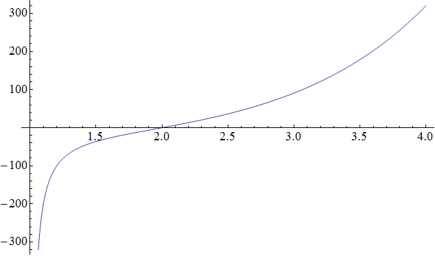
Figure 3. A graph of $F(s)$ for $1<s<4$.

5. $L^{p}$ space

Let $1\leq p\leq\infty$. We can also consider the transfer operator $L$ on the Lebesgue space $L^{p}(\mathbb{T})$. Here we consider only the case $f(t)=|\cos(\pi t)|^{q}$. Other cases can be treated similarly.

Let $d\geq 2$ be an integer. Let $L_{q}=L:L^{p}(\mathbb{T})\rightarrow L^{p}(\mathbb{T})$ be the operator given by

$$(L_{q}u)(t)=\frac{1}{d}\sum_{i=0}^{d-1}\left|\cos\left(\pi\frac{t+i}{d}\right)\right|^{q}u\left(\frac{t+i}{d}\right).$$

Then $L_{q}$ defines a bounded linear operator on $L^{p}(\mathbb{T})$. The adjoint of $L_{q}$ is given by $T_{q}=L_{q}^{*}:L^{p^{\prime}}(\mathbb{T})\rightarrow L^{p^{\prime}}(\mathbb{T})$ (where $p^{\prime}=p/(1-p)$),

$$(T_{q}x)(t)=|\cos(\pi t)|^{q}x(d\cdot t).$$

Notice that, for $p^{\prime}<\infty$,

$$\|T_{q}x\|_{p^{\prime}}^{p^{\prime}} =\int_{\mathbb{T}}|\cos(\pi t)|^{qp^{\prime}}|x(d\cdot t)|^{p^{\prime}}dt$$

$$=\int_{\mathbb{T}}(L_{qp^{\prime}}1)(t)|x(t)|^{p^{\prime}}dt.$$

Thus

$$\|L_{q}\|_{p\rightarrow p} =\|T_{q}\|_{p^{\prime}\rightarrow p^{\prime}}$$

$$=\left(\sup_{\|x\|_{p^{\prime}}\leq 1}\|T_{q}x\|_{p^{\prime}}^{p^{\prime}}\right)^{1/p^{\prime}}$$

$$=\left(\sup_{\||x|^{p^{\prime}}\|_{1}\leq 1}\int_{\mathbb{T}}(L_{qp^{\prime}}1)(t)|x(t)|^{p^{\prime}}dt\right)^{1/p^{\prime}}$$

$$=\|L_{qp^{\prime}}1\|_{\infty}^{1/p^{\prime}}.$$

By Lemma 3.2, the function $h_{1}(t)=(L_{qp^{\prime}}1)(t)$ attains its maximum at either $t=0$ or $t=1/2$ depending on the value of $qp^{\prime}$. (Note that the function $h_{1}$ for $f=|\cos(\pi t)|^{q}$ and that for $f=|\sin(\pi t)|^{q}$ differ only by a translation of $d/2$.) In particular, we obtain an explicit formula for the operator norm

$$\|L_{q}\|_{p\rightarrow p}=\max\left\{(L_{qp^{\prime}}1)(0),(L_{qp^{\prime}}1)(1/2)\right\}.$$

More generally, for any $n\in\mathbb{N}$, the same argument as above gives

$$\|L_{q}^{n}\|_{p\rightarrow p}=\|L_{qp^{\prime}}^{n}1\|_{\infty}^{1/p^{\prime}}.$$

Therefore, to compute the spectral radius of $L_{q}$ on $L^{p}(\mathbb{T})$, it suffices to find

$$\rho_{p}(L_{q}):=\lim_{n\rightarrow\infty}\|L_{q}^{n}\|^{1/n}_{p\rightarrow p} =\lim_{n\rightarrow\infty}\|L_{qp^{\prime}}^{n}1\|_{\infty}^{1/(np^{\prime})}$$

$$=\lim_{n\rightarrow\infty}\|h_{n}\|_{\infty}^{1/(np^{\prime})}$$

where $h_{n}(t)=(L_{qp^{\prime}}^{n}1)(t)$. However, the last expression is the $p^{\prime}$th root of the spectral radius of $L_{qp^{\prime}}$ on $C(\mathbb{T})$. So we obtain the following.

Proposition 5.1.

For $p>1$, we have

$$\rho_{p}(L_{q})=\big{[}\rho(L_{qp^{\prime}})\big{]}^{1/p^{\prime}}.$$

Similar as in Section 4, in the special case $d=2$, we can find eigenfunctions of $L_{q}$ in $L^{p}(\mathbb{T})$ explicitly. We consider two different cases.

Case 1: $qp^{\prime}\leq 1$. In this case we have, by Theorem 4.2,

$$\rho(L_{qp^{\prime}})=2^{-qp^{\prime}},$$

and so

$$\rho_{p}(L_{q})=2^{-q}.$$

Since $q\leq 1$, the spectral radius of $L_{q}$ on $L^{p}(\mathbb{T})$ coincides that on $C(\mathbb{T})$. In particular, we have the same eigenfunction

$$u(t)=|\sin(\pi t)|^{q}\in L^{p}(\mathbb{T})$$

corresponding to the eigenvalue $\lambda=2^{-q}$.

Case 2: $qp^{\prime}>1$. In this case we have

$$\rho(L_{qp^{\prime}})=\frac{1}{2},$$

and so

$$\rho_{p}(L_{q})=2^{-1/p^{\prime}}.$$

Note that $1/p^{\prime}<q$. Following the same idea as in Section 4, we consider functions of the form

$$u_{s}(t)=|\sin(\pi t)|^{q}G(s,t)$$

where $s>1$ and $G(s,t)=\zeta(s,t)+\zeta(s,1-t)$ is as in (28). Since

$$\zeta(s,t)\sim t^{-s},\quad\text{as }t\rightarrow 0^{+},$$

we have that $u_{s}\in L^{p}(\mathbb{T})$ if and only if $(s-q)p<1$, i.e.

$$s<q+\frac{1}{p}.$$

Since $qp^{\prime}>1$ exactly when $q+\frac{1}{p}>1$, we can take

$$s=q+\frac{1}{p}-\varepsilon$$

for sufficiently small $\varepsilon>0$ to obtain an eigenfunction in $L^{p}(\mathbb{T})$ corresponding to the eigenvalue

$$2^{-q+(s-1)}=2^{-1/p^{\prime}-\varepsilon}.$$

Therefore, as $\varepsilon\rightarrow 0$, $u_{s}(t)$ gives an ‘approximate’ eigenfunction corresponding to $\rho_{p}(L_{q})=2^{-1/p^{\prime}}$. Note that when $\varepsilon=0$, $u_{s}(t)$ gives an eigenfunction in the Lorentz space $L^{p,\infty}(\mathbb{T})$.

6. An application to Fourier multipliers

In this section, we present an application to some Bochner-Riesz type multipliers introduced by Mockenhaupt in [8, Section 4.3]. Let $E\subset\mathbb{R}$ be the middle-third Cantor set obtained from dissecting the interval $[-1/2,1/2]$, and let $\mu$ be the Cantor measure on $E$. It is well known that

$$\dim E=\alpha:=\frac{\log 2}{\log 3}$$

and that the Fourier transform of $\mu$ is given by

(33) $$\hat{\mu}(x)=\int_{\mathbb{R}}e^{-\pi ix\xi}d\mu(\xi)=\prod_{j=1}^{\infty}{\cos(\pi 3^{-j}x)}.$$

Let $\chi\in C_{c}^{\infty}(\mathbb{R})$ be a bump function with $\hat{\chi}\geq 0$. For $\delta>0$, let

$$m_{\delta}(\xi)=\frac{\chi(\cdot)}{|\cdot|^{\alpha-\delta}}*\mu(\xi)=\int_{\mathbb{R}}\frac{\chi(\xi-\eta)}{|\xi-\eta|^{\alpha-\delta}}d\mu(\eta).$$

Note that $m_{\delta}$ defines a bounded function only when $\delta>0$. In particular, $m_{\delta}$ is an $L^{2}$-Fourier multiplier if and only if $\delta>0$.

Theorem 6.1.

$m_{\delta}$ is an $L^{1}$-Fourier multiplier if and only if

$$\delta>\frac{\log 2}{\log 3}+\frac{\log c(1)}{\log 3}=0.236\cdots$$

where $c(1)$ is as in Section 3 (with $d=3$).

Proof.

Recall that an $L^{p}$-Fourier multiplier is a function $m(\xi)$ such that

(34) $$\|\mathcal{F}^{-1}\big{(}m(\xi)\hat{f}(\xi)\big{)}\|_{L^{p}(\mathbb{R})}\leq C\|f\|_{L^{p}(\mathbb{R})}$$

holds for a constant $C$ independent of $f$, where $\mathcal{F}^{-1}$ denotes the inverse Fourier transform. In the case $p=1$, this is equivalent to $\widehat{m}$ being a finite measure. If $\alpha-\delta\leq 0$, it is easy to see that this is the case with $m=m_{\delta}$. If $\alpha-\delta>0$, then we have

$$\widehat{m}_{\delta}(x)=c\cdot\left(\hat{\chi}*{|\cdot|^{\alpha-\delta-1}}\right)(x)\cdot\hat{\mu}(x)$$

for some constant $c$. Thus, ${m}_{\delta}$ is an $L^{1}$-Fourier multiplier if and only if

$$\int_{\mathbb{R}}|\widehat{m}_{\delta}(x)|dx =\int_{|x|\leq 3}|\widehat{m}_{\delta}(x)|dx+\sum_{k=1}^{\infty}\int_{3^{k}<|x|\leq 3^{k+1}}|\widehat{m}_{\delta}(x)|dx$$

$$\approx 1+\sum_{k=1}^{\infty}3^{(\alpha-\delta-1)k}\int_{3^{k}}^{3^{k+1}}\prod_{j=1}^{\infty}|{\cos(\pi 3^{-j}x)}|dx$$

$$<\infty$$

where we have used

$$\hat{\chi}*{|\cdot|^{\alpha-\delta-1}}(x)\approx|x|^{\alpha-\delta-1},\ \text{as }|x|\rightarrow\infty$$

and (33). On the other hand, notice that

$$\int_{3^{k}}^{3^{k+1}}\prod_{j=1}^{\infty}|{\cos(\pi 3^{-j}x)}|dx =3^{k}\int_{1}^{3}\prod_{j=1}^{\infty}|{\cos(\pi 3^{k-j}x)}|dx$$

$$=3^{k}\int_{1}^{3}|\hat{\mu}(x)|\prod_{j=0}^{k-1}|{\cos(\pi 3^{j}x)}|dx$$

$$\approx 3^{k}\int_{0}^{1}\prod_{j=0}^{k-1}|{\cos(\pi 3^{j}x)}|dx$$

where in the last line we have used periodicity and the fact that $|\hat{\mu}(x)|$ is bounded below on the interval $[2,3]$. Now by Theorem 2.6(b), we know that

$$\int_{0}^{1}\prod_{j=0}^{k-1}|{\cos(\pi 3^{j}x)}|dx\approx c(1)^{k}.$$

Therefore

$$\int_{\mathbb{R}}|\widehat{m}_{\delta}(x)|dx<\infty$$

if and only if

$$\sum_{k=1}^{\infty}3^{(\alpha-\delta-1)k}3^{k}c(1)^{k}<\infty,$$

which is equivalent to

$$\delta>\frac{\log 2}{\log 3}+\frac{\log c(1)}{\log 3}.$$

This completes the proof. ∎

Since $m_{\delta}$ is compactly supported, we can choose $f\in L^{p}(\mathbb{R})$ in (34) such that $\hat{f}\equiv 1$ on the support of $m=m_{\delta}$, and get $\widehat{m}_{\delta}\in L^{p}(\mathbb{R})$ as a necessary condition for $m_{\delta}$ to be an $L^{p}$-Fourier multiplier. By the same argument as above, this leads us to

$$\delta>\delta(p):=\frac{\log 2}{\log 3}-1+\frac{1}{p}+\frac{\log\big{(}c(p)^{1/p}\big{)}}{\log 3}.$$

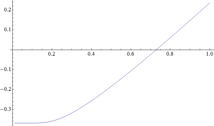
Figure 4. A graph of $\delta(p)$ as a function of $1/p\in(0,1)$.

References

- [1] Y. A. Abramovich, C. D. Aliprantis, and O. Burkinshaw. Positive operators on Kreĭn spaces. Acta Appl. Math., 27(1-2):1–22, 1992. Positive operators and semigroups on Banach lattices (Curaçao, 1990).
- [2] V. Baladi. Positive transfer operators and decay of correlations, volume 16 of Advanced Series in Nonlinear Dynamics. World Scientific Publishing Co., Inc., River Edge, NJ, 2000.
- [3] A. H. Fan and K.-S. Lau. Asymptotic behavior of multiperiodic functions . J. Fourier Anal. Appl., 4(2):129–150, 1998.
- [4] F. P. Gantmacher and M. G. Krein. Oscillation matrices and kernels and small vibrations of mechanical systems. AMS Chelsea Publishing, Providence, RI, revised edition, 2002. Translation based on the 1941 Russian original, Edited and with a preface by Alex Eremenko.
- [5] H. Hennion. Sur un théorème spectral et son application aux noyaux lipchitziens. Proc. Amer. Math. Soc., 118(2):627–634, 1993.
- [6] R. A. Horn and C. R. Johnson. Matrix analysis. Cambridge University Press, Cambridge, 1985.
- [7] P. Janardhan, D. Rosenblum, and R. S. Strichartz. Numerical experiments in Fourier asymptotics of Cantor measures and wavelets. Experiment. Math., 1(4):249–273, 1992.
- [8] G. Mockenhaupt. Bounds in Lebesgue spaces of oscillatory integral operators. Habilitationsschrift, Universität Siegen, Germany, 1996.
- [9] S. Smirnov. Notes on Ruelle’s theorem. available at http://www.unige.ch/~smirnov/papers/ruelle.pdf, 1999.
- [10] R. S. Strichartz. Self-similar measures and their Fourier transforms. I. Indiana Univ. Math. J., 39(3):797–817, 1990.
- [11] L. Vepštas. The Bernoulli map. available at http://www.academia.edu/3221320/The_bernoulli_map, 2004/2008/2010/2014.