Spheroidal harmonic expansions for the solution of Laplace’s equation for a point source near a sphere

Abstract

We propose a powerful approach to solve Laplace’s equation for point sources near a spherical object. The central new idea is to use prolate spheroidal solid harmonics, which are separable solutions of Laplace’s equation in spheroidal coordinates, instead of the more natural spherical solid harmonics. We motivate this choice and show that the resulting series expansions converge much faster. This improvement is discussed in terms of the singularity of the solution and its analytic continuation. The benefits of this approach are illustrated for a specific example: the calculation of modified decay rates of light emitters close to nanostructures in the long-wavelength approximation. We expect the general approach to be applicable with similar benefits to a variety of other contexts, from other geometries to other equations of mathematical physics.

Laplace’s equation is one of the most important partial differential equations of physics and engineering. It arises in many fields including electromagnetism, classical gravity, and fluid dynamics. It also has close links, through the Laplacian operator, with other important differential equations of physics, such as the wave equation and the diffusion equation. Analytical solutions of Laplace’s equation, typically obtained via the method of separation of variables, are standard materials for physics textbooks Morse and Feshbach (1953). The solution for a point source located outside a sphere plays a specially important role through its connection with the Green’s function formalism Stratton (1941). We will focus on electrostatics in this article, but our results naturally extend to other applications of Laplace’s equation.

The standard electrostatics solution for a point source outside a dielectric sphere is relatively straightforward and obtained as a multipole expansion (infinite series) Stratton (1941); Ford and Weber (1984). One important and often overlooked property of those series is that they can be very slowly convergent for sources close to the surface (often the most relevant situation), as shown explicitly in Ref. Le Ru and Etchegoin (2009). Moroz recently revisited this problem by focusing specifically on the decay rates (i.e. the self-field of a dipole in the quasi-static approximation) and used mathematical manipulations to express those series in a more convergent form Moroz (2011). Lindell also approached this problem from the point of view of image theory Lindell (1992), but the resulting solutions involve integrals which must be computed numerically.

In this work, we propose and demonstrate an alternative approach based on the use of spheroidal harmonics, which are the separable solutions of Laplace’s equation in spheroidal coordinates Stratton (1941); Morse and Feshbach (1953). This choice may appear counter-intuitive for a spherical object, but the point source breaks the spherical symmetry and we will show that the spheroidal harmonics are better suited to account for the singularities of the solution. With this original approach, we demonstrate dramatic improvements for the convergence of the solution series. We show that this idea is directly applicable to different types of point sources and argue that its applicability could extend to other geometries and other equations of mathematical physics.

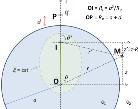
Figure 1: Schematic of the electrostatics problem under study: a point charge $q$ at a distance $d$ from a sphere of radius $a$. The various coordinate systems used in the solution are also illustrated: spherical ($r$,$\theta$,$\phi$), offset spherical ($r^{\prime}$,$\theta^{\prime}$,$\phi$), and offset prolate spheroidal ($\bar{\xi}$,$\bar{\eta}$,$\phi$).

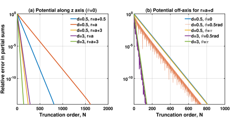
Figure 2: Convergence of the standard series solution (Eq. S32) for a point charge at a distance of $d=0.5$ nm or $d=3$ nm from an $a=25$ nm-radius sphere (with $\epsilon=-6.5+0.67i$). The relative errors in the partial sums (with respect to the converged sums) are shown for the outside potential at different positions either along the $z$-axis (a) or off-axis for $r=a+d$ (b).

To present our new approach, we will first focus on the simplest case of a point charge. As illustrated in Fig. 1, we consider a point charge $q$ located at $\mathbf{R}_{P}$, on the $z$-axis at a distance $d$ from a sphere of radius $a$ ($|\mathbf{R}_{P}|=R_{P}=a+d)$. The dielectric relative permittivities of the sphere and embedding medium are $\epsilon_{2}$ and $\epsilon_{1}$ respectively and their ratio is denoted $\epsilon={\epsilon_{2}}/{\epsilon_{1}}$ for convenience. Our results will be illustrated for $\epsilon={-6.5+0.67i}$ (corresponding to a gold sphere in water excited with $\lambda=633$ nm light in the quasi-static approximation), but similar conclusions were obtained with other values of $\epsilon$, including for absorbing or non-absorbing dielectric spheres. We also choose for illustration a sphere radius of $a=25\,$nm and a distance from the surface of $d=0.5$ or $d=3$ nm, but note that the results are scale-invariant.

We seek the outside potential $\phi(\mathbf{r})$, solution of Laplace’s equation in the presence of this source term. For convenience, we write $\phi=\bar{\phi}q/(4\pi\epsilon_{0}\epsilon_{1}a)$ and work with the dimensionless $\bar{\phi}$. The standard solution of this problem consists in expanding the point charge potential $\bar{\phi}_{q}$ as a series of regular solid harmonics centered on the sphere Stratton (1941):

$$\bar{\phi}_{q}=\frac{a}{R_{P}}\sum_{n=0}^{\infty}\frac{r^{n}}{R_{P}^{n}}P_{n}(\cos\theta)\quad(r<R_{P})$$ (1)

where $(r,\theta,\phi)$ are spherical coordinates and $P_{n}$ are the Legendre polynomials. The potential outside the sphere ($r>a$) is then given by $\bar{\phi}_{\mathrm{out}}=\bar{\phi}_{q}+\bar{\phi}_{r}$, with the “reflected” potential Stratton (1941):

$$\bar{\phi}_{r}=-\sum_{n=0}^{\infty}~{}\beta_{n}\left(\frac{R_{I}}{r}\right)^{n+1}P_{n}(\cos\theta),$$ (2)

where $R_{I}=a^{2}/R_{P}$ and the adimensional sphere polarizabilities are:

$$\beta_{n}=\frac{n(\epsilon-1)}{n(\epsilon+1)+1}.$$ (3)

We also define $\beta_{\infty}=(\epsilon-1)/(\epsilon+1)$, which is related to the response of a planar interface.

As discussed in Refs. Lindell (1992); Le Ru and Etchegoin (2009); Moroz (2011), the sum in Eq. S32 can be very slowly convergent when evaluated at or in the vicinity of the sphere surface ($r\approx a$) for a point source close to the sphere ($d\ll a$). This is shown explicitly in Fig. 2 where we computed the relative errors from the partial series of the potential at different points close to or on the sphere surface. One for example needs to sum more than 1500 terms in the series to obtain a converged solution (within the double-precision accuracy of $\sim 10^{-15}$) of the potential on the sphere surface when $a/d=50$. This slow convergence also occurs everywhere on the sphere surface, not just in the vicinity of the point source. In order to motivate our choice of working with prolate spheroidal coordinates, we first derive a more convergent formulation of the solution with spherical coordinates, where the nature of the singularities of the solution becomes more apparent. For this, we start from Eq. S32, and isolate the dominant contribution for large $n$ by writing:

$$\beta_{n} =\beta_{\infty}-\frac{\beta_{\infty}}{n(\epsilon+1)+1}.$$ (4)

Substituting back into Eq. S32, the second term gives a series that converges faster and the the first term gives a (still slowly-converging) series for which we recognize a closed-form analytical expression Stratton (1941):

$$-\beta_{\infty}\sum_{n=0}^{\infty}~{}\left(\frac{R_{I}}{r}\right)^{n+1}~{}P_{n}(\cos\theta)=-\frac{\beta_{\infty}R_{I}}{|\mathbf{r}-R_{I}\hat{\bm{z}}|}.$$ (5)

This can be viewed as the potential created by an image point charge $q_{I}=-q\beta_{\infty}(R_{I}/a)$, located at a distance $R_{I}$ from the origin on the $z$ axis (point I, see Fig. 1). This is the same image charge location as that used in the method of images to solve the same problem for a perfect conductor Stratton (1941); Jackson (1998). The solution then takes the form (the primed coordinates refer to those centered at I):

$$\bar{\phi}_{r}=-\beta_{\infty}\frac{R_{I}}{r^{\prime}}+\sum_{n=0}^{\infty}\frac{\beta_{\infty}}{n(\epsilon+1)+1}\left(\frac{R_{I}}{r}\right)^{n+1}P_{n}(\cos\theta).$$ (6)

The slow convergence of the series in Eq. S32 has been partially removed by isolating and recognizing the analytical expression for the image charge. Nevertheless, the convergence of the series in Eq. S50 remains slow (Fig. 3). This approach can be repeated to further improve the convergence. Isolating the next term and recognizing its closed-form expression, we obtain after manipulation (see Sec. S.I.):

$$\bar{\phi}_{r}=-\beta_{\infty}\frac{R_{I}}{r^{\prime}}+\frac{\beta_{\infty}}{\epsilon+1}\ln\frac{r^{\prime}-z^{\prime}}{r-z}$$

$$+\frac{\epsilon\beta_{\infty}}{\epsilon+1}\sum_{n=0}^{\infty}~{}\left(\frac{R_{I}}{r}\right)^{n+1}\frac{P_{n}(\cos\theta)}{(n+1)[n(\epsilon+1)+1]}.$$ (7)

As shown in Fig. 3, the convergence of Eq. 7 is again improved, but still requires a large number of terms ($\sim 800$) to reach double-precision accuracy.

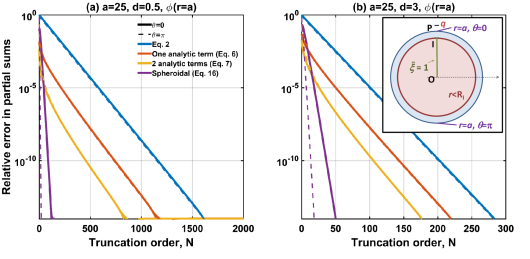
Figure 3: Convergence of the improved series solutions for the outside potential at the surface ($r=a$) either close to the source ($\theta=0$, solid lines) or at the opposite side of the sphere ($\theta=\pi$, dashed lines) for a point charge at a distance $d=0.5$ nm (a) or $d=3$ nm (b). We compare the standard solution (Eq. S32) with the improved solutions with the image charge term (Eq. S50) and with the logarithmic term (Eq. 7). The new approach using a spheroidal harmonics expansion (Eq. S45) is also compared to those and converges much faster, especially for sources very close to the sphere. The inset in (b) depicts the region of divergence of the series for spherical (red) and spheroidal (green) harmonics expansions.

It is also interesting to note that the second term in Eq. 7 exhibits a logarithmic singularity on the line segment OI; this term can therefore be viewed as an extended image source over this segment. Such a line image charge over OI was also found from a direct analysis of the problem within the method of images Lindell (1992). This extended line singularity provides the motivation for our proposed new approach to the problem. Instead of using a spherical harmonics expansion, we search instead for a solution in a basis of spheroidal harmonics, namely:

$$\bar{\phi}_{r}=\sum_{n=0}^{\infty}a_{n}Q_{n}(\bar{\xi})P_{n}(\bar{\eta}).$$ (8)

$Q_{n}(\bar{\xi})P_{n}(\bar{\eta})$ are irregular solid prolate spheroidal harmonics, i.e. they are the standard separable solutions of Laplace’s equation (where there is no $\phi$-dependence) in prolate spheroidal coordinates, with $Q_{n}(\bar{\xi})$ the Legendre functions of the second kind. $\bar{\xi}$ and $\bar{\eta}$ are prolate spheroidal coordinates with focal points at O, center of sphere, and I, position of the image charge. The segment OI then corresponds exactly to $\bar{\xi}=1$. Explicitly, $\bar{\xi}$ and $\bar{\eta}$ are:

$$\bar{\xi}=\frac{r+r^{\prime}}{R_{I}},\quad\bar{\eta}=\frac{r-r^{\prime}}{R_{I}}.$$ (9)

The “bar” notation is used here to emphasize the fact that prolate spheroidal coordinates are traditionally defined differently with O at the mid-point between the two foci Morse and Feshbach (1953). We choose these coordinates because $Q_{n}(\bar{\xi})$ is then singular exactly on the segment OI (i.e. $\bar{\xi}=1$), where the singularity of the solution is expected.

To determine the expansion coefficients $a_{n}$, we first need to find the expansion for the irregular spherical solid harmonics $P_{n}(\cos\theta)/r^{n+1}$ in terms of the irregular prolate spheroidal solid harmonics. Such expansions can be found in the literature Jansen (2000); Antonov and Baranov (2002) in the case where the spherical harmonics center is in the middle of the focal points used for the spheroidal coordinates. In our case however, the sphere center corresponds to one of the focal points, so new expressions had to be derived. The details are provided in Sec. S.II. and we here state the final result:

$${\left(\frac{R_{I}}{r}\right)^{n+1}}P_{n}(\cos\theta)=$$

$$\sum_{k=n}^{\infty}(-1)^{n+k}\frac{2(2k+1)(k+n)!}{n!^{2}(k-n)!}~{}Q_{k}(\bar{\xi})P_{k}(\bar{\eta}).$$ (10)

One can then substitute this expansion into the original solution (Eq. S32), swap the order of the sums and relabel the indices $n\leftrightarrow k$, to obtain the coefficients $a_{n}$ as:

$$a_{n}=-2(2n+1)\sum_{k=1}^{n}(-1)^{n+k}\frac{(n+k)!}{k!^{2}(n-k)!}\beta_{k}.$$ (11)

For the problem at hand, it is in fact beneficial to first isolate the point singularity (image charge) identified earlier, since it does not exhibit the line singularity found in the spheroidal solid harmonics. We therefore look for a solution of the form:

$$\bar{\phi}_{r}=-\beta_{\infty}\frac{R_{I}}{r^{\prime}}+\sum_{n=0}^{\infty}b_{n}Q_{n}(\bar{\xi})P_{n}(\bar{\eta}).$$ (12)

As for $a_{n}$, the coefficients $b_{n}$ are obtained by substituting Eq. 10 into the series in Eq. S50 and swapping the order of the sums. We obtain:

$$b_{n} =\beta_{\infty}2(2n+1)c_{n},$$ (13)

$$\mathrm{with~{}}c_{n} =\sum_{k=0}^{n}\frac{(-1)^{n+k}}{k(\epsilon+1)+1}~{}\frac{(n+k)!}{k!^{2}(n-k)!}.$$ (14)

This expression is however not suitable for practical computations as large numerical errors appear in the sum at relatively low $n$ ($\approx 20$), but one can derive the following equivalent expression (see Sec. S.III.):

$$c_{n}=\prod_{k=0}^{n}\frac{\mu-k}{\mu+k},\quad\mathrm{where~{}}\mu=\frac{1}{\epsilon+1}.$$ (15)

With this expression, $c_{n}$ can be computed easily by recurrence. The solution for the potential takes the form

$$\bar{\phi}_{r}=-\beta_{\infty}\frac{R_{I}}{r^{\prime}}+\beta_{\infty}\sum_{n=0}^{\infty}~{}2(2n+1)c_{n}Q_{n}(\bar{\xi})P_{n}(\bar{\eta}).$$ (16)

The convergence of this series is compared in Fig. 3 to those previously obtained and the improvements are dramatic. It should be noted that care should be taken in the computation of the Legendre functions of the second kind, which were computed using a backward recurrence and the modified Lentz algorithm Schneider et al. (2010). In the example of Fig. 3(a) ($a=25$, $d=0.5$), full accuracy is obtained for the surface field close to the point source with only $\sim 100$ terms instead of $\sim 1600$ for the standard solution. The benefits are even more dramatic elsewhere near the surface, with only 18 terms needed on the other side of the sphere.

To understand these improvements, we recognize that Eq. S45 provides an analytic continuation of Eq. 7. Those infinite series are strictly equivalent in the region where they both converge, but their ranges of convergence are different: Eq. 7 only converges for $r>R_{I}$, while Eq. S45 converges everywhere except on the segment OI. One naturally expects that slow convergence of either series will occur near the boundary of its region of convergence. For spheroidal expansions, the point $r=R_{P},\theta=\pi$ is far from the segment of divergence OI (see inset in Fig. 3(b)) and the series therefore converges rapidly. For spherical expansions, this point is very close to the sphere of divergence and convergence is very slow. The logarithmic term in Eq. 7 and previous studies using the method of images Lindell (1992) suggest that the analytic continuation of the solution is singular only on the segment OI and the divergence region cannot be further reduced. This suggests that the spheroidal solid harmonics (centered on the segment OI) are the most natural basis for this problem, which explains the better convergence even at the point source position, which is close to the singularity at I.

These arguments indicate that our proposed approach would be applicable to many related problems. The method can for example be adapted to apply to the solution inside the sphere (this would take us too far from the argument and will be discussed elsewhere). It can also be applied to other types of point sources near a sphere with minor modifications. We discuss below the results obtained for a dipole $\mathbf{p}$ located at a distance $d$ from the sphere on the $z$-axis (details of the derivations are provided in Secs. S.IV and S.V.). The dimensionless potential $\bar{\phi}$ is now defined as $\phi=\bar{\phi}p~{}/(4\pi\epsilon_{0}\epsilon_{1}aR_{P})$ for convenience. For a perpendicular dipole (oriented along $z$), the reflected potential can be expressed using solid spheroidal harmonics expansions as:

$$\bar{\phi}_{\bot}= \beta_{\infty}\frac{R_{I}^{2}z^{\prime}}{r^{\prime 3}}+\frac{\epsilon\beta_{\infty}}{\epsilon+1}\frac{R_{I}}{r^{\prime}}$$

$$-\frac{\epsilon\beta_{\infty}}{\epsilon+1}\sum_{n=0}^{\infty}~{}2(2n+1)c_{n}Q_{n}(\bar{\xi})P_{n}(\bar{\eta}).$$ (17)

The first two terms correspond to an image dipole and image point charge respectively, while the series exhibit a line singularity over the segment OI as before.

This solution is important in the context of nano-optics, where the modified decay rate $\Gamma$ for a dipolar emitter can be deduced from its self-field $\mathbf{E}_{\mathrm{sf}}$ as Chance et al. (1978); Ford and Weber (1984); Barnett et al. (1992); Novotny and Hecht (2006); Le Ru and Etchegoin (2009):

$$\frac{\Gamma}{\Gamma_{0}}=1+\frac{6\pi\epsilon_{0}\epsilon_{1}}{k_{1}^{3}}\frac{\mathrm{Im}\left(\mathbf{p}^{*}\cdot\mathbf{E}_{\mathrm{sf}}\right)}{|\mathbf{p}|^{2}},$$ (18)

where $\Gamma_{0}$ is the normal decay rate in the embedding medium, $k_{1}=(2\pi/\lambda)\sqrt{\epsilon_{1}}$ the wave-vector. In the quasi-static approximation, valid for spheres much smaller than the wavelength, the field solution close to the sphere can be approximated by the corresponding electrostatics solution. The self-field $\mathbf{E}_{\mathrm{sf}}$ can then be obtained by evaluating the reflected field $\mathbf{E}_{r}=-\bm{\nabla}\phi_{r}$ at the dipole position. For a dipole that is either perpendicular ($\bot$) or parallel ($\parallel$) to the sphere, we obtain (see Secs. S.IV. and S.V.):

$$\frac{\Gamma_{\bot}}{\Gamma_{0}} =1+\frac{3}{2(k_{1}a)^{3}}\mathrm{Im}\left\{\beta_{\infty}\left(\frac{2}{\delta_{P}^{3}}+\frac{\epsilon}{\epsilon+1}\frac{1}{\delta_{P}^{2}}\right.\right.$$

$$\left.\left.\times\left[1-\frac{1}{\delta_{P}(1+\delta_{P})}\sum_{n=0}^{\infty}(2n+1)(n+1)c_{n}[\bar{\xi}_{P}Q_{n}(\bar{\xi}_{P})-Q_{n+1}(\bar{\xi}_{P})]\right]\right)\right\}$$ (19)

$$\frac{\Gamma_{\parallel}}{\Gamma_{0}} =1-\frac{3}{2(k_{1}a)^{3}}\mathrm{Im}\left\{\beta_{\infty}\left(\frac{1}{\delta_{P}^{3}}-\frac{2}{\epsilon+1}\frac{1}{\sqrt{\delta_{P}(1+\delta_{P})}}\sum_{n=1}^{\infty}(2n+1)(c_{n}-1){Q_{n}^{1}(\bar{\xi}_{P})}\right)\right\}.$$ (20)

where we have defined $\delta_{P}=(R_{P}/a)^{2}-1$ ($\delta_{P}\ll 1$ when the dipole is close to the surface), $\bar{\xi}_{P}=1+2\delta_{P}$, and $Q_{n}^{m}$ are the associated Legendre functions of the second kind. Note that the coefficients $c_{n}$ in the series depend on $\epsilon$ and contribute to the material-dependence of the whole expression. In Fig. 4(a), the convergence of this new formula is compared for the perpendicular dipole to that of the standard expression obtained from spherical harmonics expansions Le Ru and Etchegoin (2009); Moroz (2011). Much faster convergence is again evidenced, and almost identical results were obtained for the parallel dipole. The wavelength dependence of the modified decay rate for a gold nanosphere is shown in Fig. 4(b) as an example of application of these new formula.

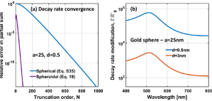
Figure 4: (a) Convergence of the standard and improved series solutions for the modified decay rates $\Gamma_{\bot}/\Gamma_{0}$. The spheroidal expansion (Eq. 19) requires much fewer terms for accurate results. (b) Spectral variation of the decay rate modification in the electrostatics approximation for a dipole perpendicular to a gold sphere of radius $a=25$ nm embedded in water ($\epsilon_{1}=1.33^{2}$), at a distance $d=0.5$ or 3 nm from the surface. The dielectric function for gold is taken from Ref. Etchegoin et al. (2006).

Beyond those examples, we envisage that our arguments could be extended to other equations of mathematical physics, such as the Helmholtz equation. The full-wave series solution for a dipole near a sphere are also slowly-convergent but the problem becomes more acute because numerical problems arise in computing those series for $n$ larger than typically 100 (the terms in the series include spherical Bessel functions whose values are beyond double-precision arithmetic at large orders). The solutions cannot therefore be easily computed numerically for dipoles close to the sphere. Spheroidal harmonics expansions (which may involve the standard spheroidal wavefunctions Li et al. (2002) or alternative definitions) may alleviate such issues. Spheroidal harmonics expansions could also provide new approaches to solve Laplace’s equation with other geometries, for example interacting spheres (where one sphere can be viewed as a source for the other) or of a sphere near an infinite plane. Although those extensions will require further developments, the results presented in this article provide a vivid demonstration of the usefulness of spheroidal coordinates in problems with symmetry of revolution where they may have been overlooked so far.

Supplimentary Information

Matt R. A. Majić Baptiste Auguié Eric C. Le Ru

I Proof of Eq. 6: closed-form expression for the logarithmic term

The same approach as carried out to find the image charge term (Eqs. 4-5) can be followed to obtain the next dominant term. We isolate the next dominant term in $\beta_{n}$ by writing:

$$\frac{n}{n(\epsilon+1)+1}=\frac{1}{\epsilon+1}-\frac{1}{(\epsilon+1)^{2}}\frac{1}{n+1}-\frac{\epsilon}{(\epsilon+1)^{2}}\frac{1}{(n+1)[n(\epsilon+1)+1]}.$$ (S1)

The choice of factor $1/(n+1)$ in the second term, instead of for example $1/n$, may look arbitrary but will simplify the calculations. When substituting back Eq. S1 into Eq. 2, the first term gives the same image charge term as found in Eq. 5. The analytic expression for the sum over the second term in Eq. S1 is less obvious. It involves the series:

$$\sum_{n=0}^{\infty}\left(\frac{R_{I}}{r}\right)^{n+1}\frac{P_{n}(\cos\theta)}{n+1}.$$ (S2)

To calculate it, we start from the generating function of the Legendre polynomials:

$$\frac{1}{\sqrt{1-2xt+t^{2}}}=\sum_{n=0}^{\infty}t^{n}P_{n}(x),\qquad(|t|<1).$$ (S3)

Integrating with respect to t:

$$\ln\left|\frac{t-x+\sqrt{1-2xt+t^{2}}}{1-x}\right|=\sum_{n=0}^{\infty}\frac{t^{n+1}}{n+1}P_{n}(x),\qquad(|t|<1).$$ (S4)

Setting $x=\cos\theta$ and $t=R_{I}/r$, we obtain after simplifications:

$$\sum_{n=0}^{\infty}\left(\frac{R_{I}}{r}\right)^{n+1}\frac{P_{n}(\cos\theta)}{n+1}=\ln\frac{r^{\prime}-z^{\prime}}{r-z}\qquad(r>R_{I}),$$ (S5)

where primed coordinates refer to the coordinates in the frame centered on point I:

$$\rho^{\prime}=\rho=r\sin\theta,\quad z^{\prime}=z-R_{I},\quad r^{\prime}=\sqrt{\rho^{2}+(z-R_{I})^{2}}=\sqrt{r^{2}-2zR_{I}+R_{I}^{2}},\quad\theta^{\prime}=\cos^{-1}\frac{z^{\prime}}{r^{\prime}}.$$ (S6)

Eq. 6 then follows for $r>R_{I}$ by substituting Eq. S1 into Eq. 2 and using the analytic forms of the series given in Eqs. 5 and S5.

It is also interesting to note that the logarithmic term found here is directly related to the prolate solid spheroidal harmonic for $n=0$:

$$Q_{0}(\bar{\xi})P_{0}(\bar{\eta})=\frac{1}{2}\ln\frac{\bar{\xi}+1}{\bar{\xi}-1}=\frac{1}{2}\ln\frac{r^{\prime}-z^{\prime}}{r-z}$$ (S7)

The latter equality is not obvious but can be proved straightforwardly by inverting the definitions of $\bar{\xi}$ and $\bar{\eta}$:

$$r=\frac{R_{I}}{2}(\bar{\xi}+\bar{\eta});\qquad r^{\prime}=\frac{R_{I}}{2}(\bar{\xi}-\bar{\eta});\qquad z=\frac{R_{I}}{2}(\bar{\xi}\bar{\eta}+1);\qquad z^{\prime}=\frac{R_{I}}{2}(\bar{\xi}\bar{\eta}-1)$$ (S8)

Then we have

$$\frac{r^{\prime}-z^{\prime}}{r-z} =\frac{(\bar{\xi}-\bar{\eta})-(\bar{\xi}\bar{\eta}-1)}{(\bar{\xi}+\bar{\eta})-(\bar{\xi}\bar{\eta}+1)}=\frac{(\bar{\xi}+1)(\bar{\eta}-1)}{(\bar{\xi}-1)(\bar{\eta}-1)}=\frac{\bar{\xi}+1}{\bar{\xi}-1}.$$ (S9)

This link (Eq. S7) provides further motivation for the use of spheroidal solid harmonics expansions.

II Expansion of spherical solid harmonics in terms of spheroidal solid harmonics

Such expansions can be found in the literature Jansen (2000); Antonov and Baranov (2002) in the case where the spherical harmonics center is in the middle of the focal points used for the spheroidal coordinates. There are four main formulae, corresponding to the expansion of regular (irregular) spherical solid harmonics in terms of regular (irregular) spheroidal harmonics and vice versa. Two of them are relevant to our problem and are reproduced below Jansen (2000); Antonov and Baranov (2002):

$$P_{n}^{m}(\xi)P_{n}^{m}(\eta) =\sum_{\begin{subarray}{c}k=m\\[2.84544pt] n+k\text{~{}even}\end{subarray}}^{n}~{}\frac{(-)^{(n-k)/2}(n+k-1)!!}{(n-k)!!(k+m)!}\frac{(n+m)!}{(n-m)!}\left(\frac{r}{c}\right)^{k}P_{k}^{m}(\cos\theta)$$ (S10)

$$\left(\frac{c}{r}\right)^{n+1}P_{n}^{m}(\cos\theta) =\sum_{\begin{subarray}{c}k=n\\[2.84544pt] n+k\text{~{}even}\end{subarray}}^{\infty}~{}\frac{(-)^{(n-k)/2+m}(2k+1)(n+k-1)!!}{(k-n)!!(n-m)!}\frac{(k-m)!}{(k+m)!}Q_{k}^{m}(\xi)P_{k}^{m}(\eta)$$ (S11)

where $(-)^{n}$ is shorthand for $(-1)^{n}$ and the foci are located at $z=\pm c$ on the $z$-axis and the prolate spheroidal coordinates for those focal points are given by (we use the definition of Ref. Morse and Feshbach (1953)):

$$\xi=\frac{\sqrt{r^{2}+2cz+r^{2}}+\sqrt{r^{2}-2cz+r^{2}}}{2c},\qquad\eta=\frac{\sqrt{r^{2}+2cz+r^{2}}-\sqrt{r^{2}-2cz+r^{2}}}{2c}.$$

In our case however, the sphere center corresponds to one of the focal points and the other one is a $z=R_{I}$, so the spheroidal coordinates are therefore given as:

$$\bar{\xi}=\frac{r+\sqrt{r^{2}-2zc+c^{2}}}{c},\qquad\bar{\eta}=\frac{r-\sqrt{r^{2}-2zc+c^{2}}}{c}.$$ (S12)

with $c\equiv R_{I}$. We therefore derived new expansions between spherical and the corresponding offset spheroidal harmonics:

$$P_{n}^{m}(\bar{\xi})P_{n}^{m}(\bar{\eta})=\frac{(n+m)!}{(n-m)!} \sum_{k=m}^{n}~{}\frac{(-)^{n+k}}{k!(k+m)!}\frac{(n+k)!}{(n-k)!}\left(\frac{r}{c}\right)^{k}P_{k}^{m}(\cos\theta)$$ (S13)

$$\frac{c^{n+1}}{r^{n+1}}P_{n}^{m}(\cos\theta)=\frac{2}{n!(n-m)!} \sum_{k=n}^{\infty}~{}(-)^{n+m+k}(2k+1)\frac{(k+n)!}{(k-n)!}\frac{(k-m)!}{(k+m)!}Q_{k}^{m}(\bar{\xi})P_{k}^{m}(\bar{\eta})$$ (S14)

The relation we use in the manuscript (Eq. 10) is Eq. S14 with $c\equiv R_{I}$ and $m=0$. It provides an expansion of the irregular solid spherical harmonics in terms of irregular spheroidal harmonics. Eq. S13 is only needed here in the proof of Eq. S14.  

Proof of Eq. S13

Let us consider the expansion of $P_{n}^{m}(\bar{\xi})P_{n}^{m}(\bar{\eta})\exp(im\phi)$ in terms of regular solid harmonics $r^{k}P_{k}^{m}(\cos\theta)\exp(im\phi)$, which must exist since the solid harmonics are a basis for regular solutions to Laplace’s equation. We can assume the $m$ are the same on both sides since $\phi$ is the same in both coordinate systems and $\exp(im\phi)$ are linearly independent functions. So we write:

$$P_{n}^{m}(\bar{\xi})P_{n}^{m}(\bar{\eta})=\sum_{k=0}^{\infty}~{}\alpha^{m}_{nk}\left(\frac{r}{c}\right)^{k}P_{k}^{m}(\cos\theta).$$ (S15)

The associated Legendre functions (see definitions in Sec. VI) can be written as

$$P_{n}^{m}(x)=\begin{cases}(-)^{m}(1-x^{2})^{m/2}\Pi_{n}^{m}(x)&|x|<1\\ (x^{2}-1)^{m/2}\Pi_{n}^{m}(x)&|x|>1\\ \end{cases}\qquad\text{, where }\Pi_{n}^{m}(x)=\frac{\mathrm{d}^{m}}{\mathrm{d}x^{m}}P_{n}(x).$$ (S16)

Using the following relation:

$$(1-\bar{\eta}^{2})(\bar{\xi}^{2}-1)=\frac{4r^{2}}{c^{2}}\sin^{2}\theta$$ (S17)

we deduce

$$P_{n}^{m}(\bar{\xi})P_{n}^{m}(\bar{\eta})=(-)^{m}\left(\frac{2r}{c}\right)^{m}\sin^{m}\theta~{}\Pi_{n}^{m}(\bar{\xi})\Pi_{n}^{m}(\bar{\eta})$$ (S18)

Eq. S15 can therefore be written in terms of $\Pi_{n}^{m}$ as

$$\Pi_{n}^{m}(\bar{\xi})\Pi_{n}^{m}(\bar{\eta})=\sum_{k=m}^{\infty}~{}\alpha^{m}_{nk}\left(\frac{r}{c}\right)^{k-m}\frac{1}{2^{m}}\Pi_{k}^{m}(\cos\theta)$$ (S19)

The coefficients $\alpha^{m}_{nk}$ can be determined by evaluating the expansion for $\theta=0$ and $r>c,z>c$, which implies $\bar{\eta}=1$ and $r=c(\bar{\xi}+1)/2$. Using the special value:

$$\Pi_{n}^{m}(1)=\frac{1}{2^{m}}\frac{(n+m)!}{m!(n-m)!}$$ (S20)

we obtain:

$$\Pi_{n}^{m}(\bar{\xi})=\sum_{k=0}^{\infty}~{}\alpha^{m}_{nk}\frac{(k+m)!(n-m)!}{(k-m)!(n+m)!}\frac{1}{2^{m}}\left(\frac{\bar{\xi}+1}{2}\right)^{k-m}.$$ (S21)

We then use the following identity for the Legendre polynomials

$$P_{n}(x)=\sum_{k=0}^{n}~{}(-)^{n+k}\frac{(n+k)!}{k!^{2}(n-k)!}\left(\frac{x+1}{2}\right)^{k}.$$ (S22)

By differentiating w.r.t $x$, $m$ times, we get

$$\Pi_{n}^{m}(x)=\sum_{k=m}^{n}~{}(-)^{n+k}\frac{(n+k)!}{k!^{2}(n-k)!}\frac{k!}{2^{m}(k-m)!}\left(\frac{x+1}{2}\right)^{k-m}.$$ (S23)

From this, we identify

$$\alpha^{m}_{nk}=\frac{(n+m)!}{(n-m)!}~{}(-)^{n+k}\frac{(n+k)!}{k!(n-k)!(k+m)!}\quad\mathrm{for~{}}m\leq k\leq n,\quad 0\mathrm{~{}otherwise,}$$ (S24)

which proves Eq. S13. Note that since the expansion is finite, it converges everywhere and is valid in all space.

Proof of Eq. S14

To prove Eq. S14, we will make use of the expansions of Green’s function in terms of both spherical and spheroidal solid harmonics. The expansion in terms of spheroidal harmonics can be found for example in Ref. Jansen (2000) for standard prolate spheroidal coordinates and it can be adapted to our modified coordinates with a simple scaling factor of 2, which comes from shrinking the focal length of the coordinates from $2c$ to $c$. For two points $\mathbf{r}_{1}$ and $\mathbf{r}_{2}$ with spheroidal coordinates denoted $(\bar{\xi}_{1},\bar{\eta}_{1},\phi_{1})$ and $(\bar{\xi}_{2},\bar{\eta}_{2},\phi_{2})$, we have when $\bar{\xi}_{1}<\bar{\xi}_{2}$:

$$\frac{1}{|\mathbf{r}_{1}-\mathbf{r}_{2}|}=\sum_{k=0}^{\infty}2\frac{2k+1}{c}\sum_{m=0}^{k}(-)^{m}(2-\delta_{m0})\frac{(k-m)!^{2}}{(k+m)!^{2}}P_{k}^{m}(\bar{\xi}_{1})P_{k}^{m}(\bar{\eta}_{1})Q_{k}^{m}(\bar{\xi}_{2})P_{k}^{m}(\bar{\eta}_{2})\cos m(\phi_{1}-\phi_{2}).$$ (S25)

We can write a similar expansion with spherical solid harmonics Jackson (1998) when $r_{1}<r_{2}$:

$$\frac{1}{|\mathbf{r}_{1}-\mathbf{r}_{2}|}=\sum_{n=0}^{\infty}\frac{r_{1}^{n}}{r_{2}^{n+1}}\sum_{m=0}^{n}(2-\delta_{m0})\frac{(n-m)!}{(n+m)!}P_{n}^{m}(\cos\theta_{1})P_{n}^{m}(\cos\theta_{2})\cos m(\phi_{1}-\phi_{2})$$ (S26)

where $(r_{1},\theta_{1},\phi_{1})$ and $(r_{2},\theta_{2},\phi_{2})$ are the spherical coordinates of $\mathbf{r}_{1}$ and $\mathbf{r}_{2}$. We then substitute Eq. S13 for $\mathbf{r_{1}}$ into Eq. S25 to express it as an expansion on the same spherical harmonics basis:

$$\frac{1}{|\mathbf{r}_{1}-\mathbf{r}_{2}|} =\sum_{k=0}^{\infty}2\frac{2k+1}{c}\sum_{m=0}^{k}(-)^{m}(2-\delta_{m0})\frac{(k-m)!^{2}}{(k+m)!^{2}}\left(\frac{(k+m)!}{(k-m)!}\sum_{n=m}^{k}~{}\frac{(-)^{k+n}}{n!(n+m)!}\frac{(k+n)!}{(k-n)!}\frac{r_{1}^{n}}{c^{n}}P_{n}^{m}(\cos\theta_{1})\right)$$

$$\hskip 142.26378pt\times Q_{k}^{m}(\bar{\xi}_{2})P_{k}^{m}(\bar{\eta}_{2})\cos m(\phi_{1}-\phi_{2}).$$

$$=\sum_{n=0}^{\infty}\sum_{m=0}^{n}\sum_{k=n}^{\infty}2\frac{2k+1}{c}(2-\delta_{m0})\frac{(-)^{n+k+m}(k-m)!(k+n)!}{(k+m)!(k-n)!n!(n+m)!}\frac{r_{1}^{n}}{c^{n}}P_{n}^{m}(\cos\theta_{1})Q_{k}^{m}(\bar{\xi}_{2})P_{k}^{m}(\bar{\eta}_{2})\cos m(\phi_{1}-\phi_{2}).$$ (S27)

where we have swapped the order of the sums using first $\sum_{m=0}^{k}\sum_{n=m}^{k}=\sum_{n=0}^{k}\sum_{m=0}^{n}$ and then
$\sum_{k=0}^{\infty}\sum_{n=0}^{k}=\sum_{n=0}^{\infty}\sum_{k=n}^{\infty}$.

Because the functions $r_{1}^{n}P_{n}^{m}(\cos\theta_{1})\cos m(\phi_{1}-\phi_{2})$ are linearly independent, we can equate all terms with same $n$ and $m$ in Eqs. S26 and S27 to get:

$$\frac{1}{r_{2}^{n+1}}\frac{(n-m)!}{(n+m)!}P_{n}^{m}(\cos\theta_{2})=\sum_{k=n}^{\infty}2\frac{2k+1}{c}\frac{(-)^{n+k+m}(k-m)!(k+n)!}{(k+m)!(k-n)!n!(n+m)!}\frac{1}{c^{n}}Q_{k}^{m}(\bar{\xi}_{2})P_{k}^{m}(\bar{\eta}_{2}),$$ (S28)

which can be simplified to obtain Eq. S14. This expansion is valid everywhere except on the line segment between the foci at $z=0$ and $z=c$.

III Simplification of coefficients $c_{n}$: proof of Eq. 15

We recall the definition of $c_{n}$ (Eq. 14) for $n\geq 0$:

$$c_{n}=\sum_{k=0}^{n}\frac{(-)^{n+k}}{k(\epsilon+1)+1}\frac{(n+k)!}{(n-k)!k!^{2}}=\mu\sum_{k=0}^{n}\frac{(-)^{n+k}}{k+\mu}\frac{(n+k)!}{(n-k)!k!^{2}}\quad\mathrm{with~{}}\mu=\frac{1}{\epsilon+1}.$$ (S29)

We want to prove that

$$\sum_{k=0}^{n}\frac{(-)^{k}}{k+\mu}\frac{(n+k)!}{(n-k)!k!^{2}}=\frac{(-)^{n}}{\mu}\prod_{k=0}^{n}\frac{\mu-k}{\mu+k}=\frac{(1-\mu)(2-\mu)...(n-\mu)}{\mu(\mu+1)(\mu+2)...(\mu+n)}.$$ (S30)

for a general $\mu$. We first convert the l.h.s into a single fraction:

$$\mathrm{l.h.s} =\frac{1}{\mu}-\frac{(n+1)n}{\mu+1}+\frac{(n+2)(n+1)n(n-1)}{(\mu+2)2!^{2}}-\frac{(n+3)(n+2)(n+1)n(n-1)(n-2)}{(\mu+3)3!^{2}}+...+(-)^{n}\frac{2n(2n-1)...1}{(\mu+n)n!^{2}}$$

$$= \frac{(\mu+1)...(\mu+n)-(n+1)n\alpha(\mu+2)(\mu+3)...(\mu+n)+\frac{1}{2!^{2}}(n+2)(n+1)n(n-1)\mu(\mu+1)(\mu+3)...(\mu+n)-...}{\mu(\mu+1)(\mu+2)...(\mu+n)}$$

Both the left and right hand sides of Eq. S30 are then fractions with the same denominator $\mu(\mu+1)(\mu+2)...(\mu+n)$, and their numerators are polynomials of $\mu$ of degree $n$. These will be equal if they are equal at $n+1$ different points. Define $f(\mu)$ as the l.h.s numerator and $g(\mu)$ as the r.h.s numerator. Choose the $n+1$ points to be at $\mu=-q$ where $q=0,1,2,...n$. For $g(\mu)$ it is easy to show that

$$g(-q)=(1+q)(2+q)...(n+q)=\frac{(n+q)!}{q!}.$$

For $f(\mu)$, note that it is composed of a sum of terms of the form $[(-)^{b}/b!^{2}]\mu(\mu+1)...(\mu+b-1)(\mu+b+1)...(\mu+n)\times(n+b)(n+b-1)...(n-b+1)$ for some $b\in\{0,1,...n\}$. When you set $\mu=-q$, all terms vanish except the $(q+1)^{\mathrm{th}}$ one. This term is:

$$f(-q) =(-)^{q}\frac{1}{q!^{2}}(n+q)(n+q-1)...(n-q+1)\times(-q)(-q-1)...(-)\times(1)(2)...(n-q)$$

$$=\frac{(n+q)!}{q!}.$$

This applies to all $n+1$ values of $q$, so $f(\mu)=g(\mu)$, which proves Eq. S30 (Eq. 15 of the manuscript).

IV Perpendicular dipole near a sphere

IV.1 Standard solution in spherical coordinates

We consider a dipole $\mathbf{p}=p\hat{\mathbf{z}}$ located at $\mathbf{R}_{P}$, on the $z$-axis at a distance $d$ from a sphere centred at the origin (i.e. $|\mathbf{R}_{P}|=R=a+d)$. For convenience, the dimensionless potential $\bar{\phi_{\perp}}$ is defined as $\phi=\bar{\phi_{\perp}}p/(4\pi\epsilon_{0}\epsilon_{1}aR_{P})$. The standard solution of this problem consists of expanding the dipole potential $\bar{\phi}_{\mathrm{dip}-{\bot}}$ as a series of regular solid harmonics centered at the origin:

$$\bar{\phi}_{\mathrm{dip}-{\bot}}(\mathbf{r})=aR_{P}\frac{z-R_{P}}{|\mathbf{r}-R_{P}\hat{\mathbf{z}}|^{3}}=-\frac{a}{R_{P}}\sum_{n=0}^{\infty}~{}(n+1)\left(\frac{r}{R_{P}}\right)^{n}P_{n}(\cos\theta)\quad(r<R_{P}).$$ (S31)

The potential outside the sphere is $\phi_{\mathrm{out}-\bot}=\bar{\phi}_{\mathrm{dip}-{\bot}}+\bar{\phi}_{\bot}$ with the reflected potential $\bar{\phi}_{\bot}(\mathbf{r})$ Stratton (1941):

$$\bar{\phi}_{\bot}=\sum_{n=1}^{\infty}~{}(n+1)\beta_{n}\left(\frac{R_{I}}{r}\right)^{n+1}P_{n}(\cos\theta),$$ (S32)

where $\beta_{n}$ are the adimensional sphere polarizabilities defined in Eq. 3.

The electrostatic field can then be obtained from

$$\mathbf{E}_{\bot}=-\bm{\nabla}\phi_{\bot}=-\frac{\partial\phi_{\bot}}{\partial r}\hat{\bm{r}}-\frac{1}{r}\frac{\partial\phi_{\bot}}{\partial\theta}\hat{\bm{\theta}}-\frac{1}{r\sin\theta}\frac{\partial\phi_{\bot}}{\partial\phi}\hat{\bm{\phi}}~{}~{}=-E_{0}R_{I}\bm{\nabla}\bar{\phi}_{\bot},\qquad\mathrm{with~{}~{}}E_{0}=\frac{p}{4\pi\epsilon_{0}\epsilon_{1}a^{3}}.$$

This gives

$$\mathbf{E}_{{\bot}}(\mathbf{r})=E_{0}\sum_{n=1}^{\infty}~{}(n+1)\beta_{n}\left(\frac{a^{2}}{R_{P}r}\right)^{n+2}\left[(n+1)P_{n}(\cos\theta)\hat{\bm{r}}-\frac{\mathrm{d}}{\mathrm{d}\theta}\left[P_{n}(\cos\theta)\right]\hat{\bm{\theta}}\right],$$ (S33)

The self-field at the dipole position ($r=R_{P}$, $\theta=0$) is then

$$\mathbf{E}_{\mathrm{sf}-{\bot}} =E_{0}\sum_{n=1}^{\infty}~{}(n+1)^{2}\beta_{n}\left(\frac{a^{2}}{R_{P}^{2}}\right)^{n+2}\hat{\bm{z}}.$$ (S34)

From this, we can use Eq. 18 to deduce the modified decay rate in the electrostatics approximation Moroz (2011); Le Ru and Etchegoin (2009):

$$\frac{\Gamma_{\bot}}{\Gamma_{0}}=1+\frac{3}{2(k_{1}a)^{3}}\sum_{n=1}~{}(n+1)^{2}\mathrm{Im}(\beta_{n})\left(\frac{a^{2}}{R_{P}^{2}}\right)^{n+2}.$$ (S35)

IV.2 Analytic expressions for image sources

We start from the reflected potential for a perpendicular dipole given in Eq. S32. Writing $\beta_{n}$ explicitly, it can be rewritten as:

$$\bar{\phi}_{\bot}=(\epsilon-1)\sum_{n=0}^{\infty}\frac{n(n+1)}{n(\epsilon+1)+1}\left(\frac{R_{I}}{r}\right)^{n+1}P_{n}(\cos\theta)$$ (S36)

We then isolate the first two dominant terms in the fraction (as $n\rightarrow\infty$):

$$\frac{n(n+1)}{n(\epsilon+1)+1}=\frac{n}{\epsilon+1}+\frac{\epsilon}{(\epsilon+1)^{2}}-\frac{\epsilon}{(\epsilon+1)^{2}[n(\epsilon+1)+1]}$$ (S37)

The sum over the second term on the r.h.s in Eq. S37 is the same as found for the point charge (Eq. 5) and can be evaluated analytically for $r>R_{I}$:

$$\sum_{n=0}^{\infty}\left(\frac{R_{I}}{r}\right)^{n+1}P_{n}(\cos\theta)=\frac{R_{I}}{r^{\prime}}.$$ (S38)

This is proportional to the potential created by an image point charge located at I.

Eq. S38 may be recognized as the expression for translation of solid spherical harmonics along the $z$ axis Jackson (1998) and can be proved using the generating function of the Legendre polynomials Abramovitz. A similar expression exists for the sum over the first term. It can be obtained by differentiating Eq. S38 with respect to $z$. First note that for $n\geq 0$:

$$\frac{\partial}{\partial z}\left[\left(\frac{R_{I}}{r}\right)^{n+1}P_{n}(\cos\theta)\right]=-\frac{n+1}{R_{I}}\left(\frac{R_{I}}{r}\right)^{n+2}P_{n+1}(\cos\theta)$$ (S39)

Then by applying $R_{I}\partial_{z}$ to both sides of equation S38 and re-indexing the sum from $n$ to $n-1$ we obtain:

$$\sum_{n=0}^{\infty}n\left(\frac{R_{I}}{r}\right)^{n+1}P_{n}(\cos\theta)=\left(\frac{R_{I}}{r^{\prime}}\right)^{2}\cos\theta^{\prime}=R_{I}^{2}\frac{z^{\prime}}{r^{\prime 3}}$$ (S40)

which is proportional to the potential of an image dipole located at I oriented along $z$ Jackson (1998), and provides an analytic expression for the sum over the first term on the r.h.s of Eq. S37. By substituting Eq. S37 into Eq. S36 and using the analytic forms of the series given in Eqs. S38,S40, we obtain:

$$\bar{\phi}_{{\bot}}=\beta_{\infty}\frac{R_{I}^{2}z^{\prime}}{r^{\prime 3}}+\frac{\epsilon\beta_{\infty}}{\epsilon+1}\frac{R_{I}}{r^{\prime}}-\frac{\epsilon\beta_{\infty}}{(\epsilon+1)}\sum_{n=0}^{\infty}~{}\left(\frac{R_{I}}{r}\right)^{n+1}\frac{1}{n(\epsilon+1)+1}P_{n}(\cos\theta).$$ (S41)

The same approach can be followed to obtain the next image source by splitting off the next leading order ($1/(n+1)$ dependence) of $\beta_{n}$. In fact this term is the same logarithmic source that was obtained for the point charge. Because it is singular on the segment OI, we do not separate it and include it in the expansion in terms of spheroidal harmonics.

IV.3 New approach with spheroidal harmonics

Following the same logic as in the manuscript for a point charge, we search for an equivalent solution where we keep the image point source terms (there are two of them here) and express the rest as a spheroidal solid harmonics expansion:

$$\bar{\phi}_{{\bot}}= R_{I}^{2}\beta_{\infty}\frac{z^{\prime}}{r^{\prime 3}}+\frac{\epsilon\beta_{\infty}}{\epsilon+1}\frac{R_{I}}{r^{\prime}}+\sum_{n=0}~{}d_{n}Q_{n}(\bar{\xi})P_{n}(\bar{\eta}).$$ (S42)

The coefficients $d_{n}$ are again obtained by substituting Eq. 10 into the series in Eq. S41 and swapping the order of the sums. We obtain:

$$d_{n} =-\beta_{\infty}\frac{\epsilon}{\epsilon+1}2(2n+1)\sum_{k=0}^{n}\frac{(-1)^{n+k}}{k(\epsilon+1)+1}~{}\frac{(n+k)!}{k!^{2}(n-k)!}=-\beta_{\infty}\frac{\epsilon}{\epsilon+1}2(2n+1)c_{n},$$ (S43)

where $c_{n}$ has been defined in Eqs. 14 and 15.

The new potential solution then takes the form:

$$\bar{\phi}_{{\bot}}=\beta_{\infty}R_{I}^{2}\frac{z^{\prime}}{r^{\prime 3}}+\frac{\epsilon\beta_{\infty}}{\epsilon+1}\frac{R_{I}}{r^{\prime}}-2\frac{\epsilon\beta_{\infty}}{\epsilon+1}\sum_{n=0}^{\infty}~{}(2n+1)c_{n}Q_{n}(\bar{\xi})P_{n}(\bar{\eta}).$$ (S45)

IV.4 Electric field and modified decay rate with new formulation

From this latest expression, we can deduce the corresponding electric field: For convenience, we provide explicit expressions for the components of the electric field. Note that multiple coordinates can be used ($r$, $\theta$, $r^{\prime}$, $\theta^{\prime}$, $\bar{\xi}$, $\bar{\eta}$) to express the field differently. We chose for simplicity to keep expressions involving a mixture of those coordinates. These are:

$$E_{\bot}^{r} =E_{0}\beta_{\infty}\left[\left(2\frac{R_{I}^{3}}{r^{\prime 3}}\cos\theta-3\frac{R_{I}^{4}r}{r^{\prime 5}}\sin^{2}\theta\right)-\frac{\epsilon}{\epsilon+1}\frac{R_{I}^{2}}{r^{\prime 3}}(R_{I}\cos\theta-r)\right.$$

$$\qquad\left.-\frac{2\epsilon}{\epsilon+1}\frac{R_{I}}{r}\sum_{n=0}^{\infty}(2n+1)(n+1)c_{n}\left(Q_{n}(\bar{\xi})P_{n}(\bar{\eta})+\frac{Q_{n}(\bar{\xi})P_{n+1}(\bar{\eta})-Q_{n+1}(\bar{\xi})P_{n}(\bar{\eta})}{\bar{\xi}-\bar{\eta}}\right)\right]$$

$$E_{\bot}^{\theta} =E_{0}\beta_{\infty}\sin\theta\left[\frac{R_{I}^{3}(r^{2}+R_{I}z-2R_{I}^{2})}{r^{\prime 5}}+\frac{\epsilon}{\epsilon+1}\frac{R_{I}^{3}}{r^{\prime 3}}\right.$$

$$\qquad\left.-\frac{2\epsilon}{\epsilon+1}\frac{R_{I}}{r}\sin\theta\sum_{n=0}^{\infty}(2n+1)(n+1)c_{n}\left(\frac{Q_{n}(\bar{\xi})P_{n}(\bar{\eta})\cos\theta}{\sin^{2}\theta}+\frac{r}{r^{\prime}}\left(\frac{Q_{n}(\bar{\xi})P_{n+1}(\bar{\eta})}{\bar{\eta}^{2}-1}-\frac{Q_{n+1}(\bar{\xi})P_{n}(\bar{\eta})}{\bar{\xi}^{2}-1}\right)\right)\right]$$

$$E_{\bot}^{\phi} =0$$ (S46)

The dipole position corresponds to coordinates

$$r=R_{P}, \theta=0,$$

$$r^{\prime}=R_{P}-R_{I}=R_{I}\delta_{P}, \theta^{\prime}=0,$$

$$\bar{\xi}=\bar{\xi}_{P}=2\frac{R_{P}^{2}}{a^{2}}-1=1+2\delta_{P}, \bar{\eta}=1,$$

$$\mathrm{where~{}~{}}\delta_{P}=\frac{R_{P}^{2}}{a^{2}}-1.$$

Note that the adimensional parameter $\delta_{P}>0$ becomes small when the dipole is close to the surface. The self-field $\bm{E}_{\mathrm{sf}-{\bot}}$ (at the dipole position) is given by

$$\bm{E}_{\mathrm{sf}-{\bot}} =E_{0}\beta_{\infty}\left(\frac{2}{\delta_{P}^{3}}+\frac{\epsilon}{\epsilon+1}\frac{1}{\delta_{P}^{2}}\left[1-\frac{1}{\delta_{P}(1+\delta_{P})}\sum_{n=0}^{\infty}(2n+1)(n+1)c_{n}[\bar{\xi}_{P}Q_{n}(\bar{\xi}_{P})-Q_{n+1}(\bar{\xi}_{P})]\right]\right)\hat{\bm{z}}$$ (S47)

from which we deduce the modified decay rate as

$$\frac{\Gamma_{\bot}}{\Gamma_{0}}=1+\frac{3}{2(k_{1}a)^{3}}\mathrm{Im}\left\{\beta_{\infty}\left(\frac{2}{\delta_{P}^{3}}+\frac{\epsilon}{\epsilon+1}\frac{1}{\delta_{P}^{2}}\left[1-\frac{1}{\delta_{P}(1+\delta_{P})}\sum_{n=0}^{\infty}(2n+1)(n+1)c_{n}[\bar{\xi}_{P}Q_{n}(\bar{\xi}_{P})-Q_{n+1}(\bar{\xi}_{P})]\right]\right)\right\}$$ (S48)

It is worth noting that the coefficients $c_{n}$ in the series also depend on $\epsilon$ and contribute to the material-dependence of the whole expression.

V Parallel dipole near a sphere

In this section, we adapt the derivations presented for the perpendicular dipole to the case of a parallel dipole. The main difference is that all spherical and spheroidal harmonic expansions now contain Legendre functions $P_{n}^{m},~{}Q_{n}^{m}$ with $m=1$, instead of $m=0$ for perpendicular dipoles.

V.1 Solution in spherical coordinates

The standard solution of this problem consists of expanding the dipole potential as a series of regular solid harmonics centred at the origin. For a dipole along $x$, located on the $z$-axis at $z=R_{P}$, we have (analogous to Eq. S31):

$$\bar{\phi}_{\mathrm{dip}-{\parallel}}=\frac{aR_{P}x}{|\mathbf{r}-R_{P}\hat{\mathbf{z}}|^{3}}=-\frac{a}{R_{P}}\sum_{n=1}^{\infty}~{}\left(\frac{r}{R_{P}}\right)^{n}P^{1}_{n}(\cos\theta)\cos\phi\qquad(r<R_{P}).$$ (S49)

The solution of the problem outside the sphere ($r>a$) is then given by $\bar{\phi}_{\mathrm{out-||}}=\bar{\phi}_{\mathrm{dip}-{\parallel}}+\bar{\phi}_{{\parallel}}$, with the reflected potential $\bar{\phi}_{{\parallel}}$ given by Stratton (1941):

$$\bar{\phi}_{{\parallel}}=\sum_{n=1}^{\infty}~{}\beta_{n}\left(\frac{R_{I}}{r}\right)^{n+1}~{}P_{n}^{1}(\cos\theta)\cos\phi,$$ (S50)

where $\beta_{n}$ are the adimensional sphere polarizabilities as defined in Eq. 3.

The reflected electric field solution outside the sphere is then:

$$\mathbf{E}_{\parallel}=E_{0}\sum_{n=1}^{\infty}\beta_{n}\left(\frac{R_{I}}{r}\right)^{n+2}\left[(n+1)P_{n}^{1}(\cos\theta)\cos\phi\hat{\bm{r}}-\frac{\mathrm{d}}{\mathrm{d}\theta}\left[P_{n}^{1}(\cos\theta)\right]\cos\phi\hat{\bm{\theta}}+\frac{P_{n}^{1}(\cos\theta)}{\sin\theta}\sin\phi\hat{\bm{\phi}}\right]$$

where $E_{0}=p/(4\pi\epsilon_{0}\epsilon_{1}a^{3})$. To calculate the self-field $E_{\mathrm{sf}-{\parallel}}$ (at $r=R_{P}$, $\theta=0$), we need to take the limit as $\theta\rightarrow 0$. We use the equalities:

$$P_{n}^{1}(1)=0,\quad\lim_{\theta\rightarrow 0}\left[\sin\theta{\frac{\mathrm{d}}{\mathrm{d}\theta}P_{n}^{1}(\cos\theta)}\right]=\lim_{\theta\rightarrow 0}\left[\frac{P_{n}^{1}(\cos\theta)}{\sin\theta}\right]=-\frac{n(n+1)}{2},$$ (S51)

and

$$\hat{\bm{x}}=\sin\theta\cos\phi\hat{\bm{r}}+\cos\theta\cos\phi\hat{\bm{\theta}}-\sin\phi\hat{\bm{\phi}}$$ (S52)

to obtain

$$\mathbf{E}_{\mathrm{sf}-{\parallel}} =E_{0}\sum_{n=1}^{\infty}\frac{n(n+1)}{2}\beta_{n}\left(\frac{a^{2}}{R_{P}^{2}}\right)^{n+2}\hat{\bm{x}}.$$ (S53)

The modified decay rate is therefore

$$\frac{\Gamma_{\parallel}}{\Gamma_{0}}=1+\frac{3}{4(k_{1}a)^{3}}\sum_{n=1}^{\infty}n(n+1)\mathrm{Im}(\beta_{n})\left(\frac{a^{2}}{R_{P}^{2}}\right)^{n+2}.$$ (S54)

V.2 Analytic expressions for image terms

We now come back to the potential (Eq. S50). Following the same arguments as for the perpendicular dipole, one can recognize closed-form expressions for the first few dominant terms. $\beta_{n}$ can be split and analytic expressions for the series can be identified. Explicitly:

$$\frac{n}{n(\epsilon+1)+1}=\frac{1}{\epsilon+1}-\frac{1}{n(\epsilon+1)^{2}}+\frac{1}{n(\epsilon+1)^{2}(n\epsilon+n+1)}.$$ (S55)

The first term results in the series

$$\sum_{n=1}^{\infty}~{}\left(\frac{R_{I}}{r}\right)^{n+1}P_{n}^{1}(\cos\theta)\cos\phi=-R_{I}^{2}\frac{x^{\prime}}{r^{\prime 3}}$$ (S56)

where we have recognized the expansion of a dipole offset along the $z$-axis (and located at $z=R_{I}$). This is the image dipole, whose orientation is in this case opposite to the real dipole.

The second term gives the series:

$$\sum_{n=1}^{\infty}\frac{1}{n}\left(\frac{R_{I}}{r}\right)^{n+1}P_{n}^{1}(\cos\theta)\cos\phi$$ (S57)

In contrast with the case of a perpendicular dipole where an image point charge was identified, it is not straightforward here to recognize an analytic expression. To develop this further, we will use (for $n\geq 1$):

$$P_{n}^{1}(\cos\theta)=\frac{n}{\sin\theta}[\cos\theta P_{n}(\cos\theta)-P_{n-1}(\cos\theta)].$$ (S58)

We then have

$$\sum_{n=1}^{\infty}\frac{1}{n}\left(\frac{R_{I}}{r}\right)^{n+1}P_{n}^{1}(\cos\theta)\cos\phi =\frac{\cos\phi}{\sin\theta}\sum_{n=1}^{\infty}\left(\frac{R_{I}}{r}\right)^{n+1}(\cos\theta P_{n}-P_{n-1})$$

$$=\frac{\cos\phi}{\sin\theta}\left[\cos\theta\sum_{n=1}^{\infty}\left(\frac{R_{I}}{r}\right)^{n+1}P_{n}-\frac{R_{I}}{r}\sum_{n=0}^{\infty}\left(\frac{R_{I}}{r}\right)^{n+1}P_{n}\right]$$

$$=\frac{\cos\phi}{\sin\theta}\left[\cos\theta\left(\frac{R_{I}}{r^{\prime}}-\frac{R_{I}}{r}\right)-\frac{R_{I}}{r}\frac{R_{I}}{r^{\prime}}\right]\qquad\mathrm{using~{}Eq.~{}\ref{gf_formula}}$$

$$=\frac{R_{I}\cos\phi}{r\sin\theta}(\cos\theta^{\prime}-\cos\theta)\qquad\mathrm{~{}~{}~{}~{}since~{}}\cos\theta^{\prime}=\frac{r\cos\theta-R_{I}}{r^{\prime}}$$

$$=\frac{R_{I}x}{\rho^{2}}(\cos\theta^{\prime}-\cos\theta)$$ (S59)

Note that the above expression is singular on the line from O to I, but converges to a finite value elsewhere even on the $z$ axis.

Putting those results together, and using $x^{\prime}=x$, we have for the potential:

$$\bar{\phi}_{\parallel}=-\beta_{\infty}\frac{R_{I}^{2}x}{r^{\prime 3}}-\frac{\beta_{\infty}}{\epsilon+1}\frac{R_{I}x(\cos\theta^{\prime}-\cos\theta)}{r^{2}\sin^{2}\theta}+\frac{\beta_{\infty}}{\epsilon+1}\cos\phi\sum_{n=1}^{\infty}\left(\frac{R_{I}}{r}\right)^{n+1}\frac{P^{1}_{n}(\cos\theta)}{n(n(\epsilon+1)+1)}$$ (S60)

V.3 New approach with spheroidal harmonics

The main difference with the perpendicular dipole is that only the first dominant analytic term in the expression above is a point singularity. Since the second term exhibits the line singularity from O to I, there is no reason to isolate it when looking for the expansion in spheroidal harmonics. We therefore start from the potential with the image dipole term only, namely:

$$\bar{\phi}_{\parallel}=-\beta_{\infty}\frac{R_{I}^{2}x}{r^{\prime 3}}-\beta_{\infty}\cos\phi\sum_{n=1}^{\infty}\left(\frac{R_{I}}{r}\right)^{n+1}\frac{P^{1}_{n}(\cos\theta)}{n(\epsilon+1)+1}$$ (S61)

This can then be converted into a spheroidal solid harmonics expansion using Eq. S14 for $m=1$, which reads:

$$\left(\frac{R_{I}}{r}\right)^{n+1}P^{1}_{n}(\cos\theta)=-2\sum_{k=n}^{\infty}\frac{(-)^{n+k}}{n!(n-1)!}\frac{(k+n)!}{(k-n)!}\frac{2k+1}{k(k+1)}Q_{k}^{1}(\bar{\xi})P_{k}^{1}(\bar{\eta})$$ (S62)

The series in the previous equation for $\bar{\phi}_{\parallel}$ then becomes

$$\sum_{n=1}^{\infty}\frac{P^{1}_{n}(\cos\theta)}{n(\epsilon+1)+1}\left(\frac{R_{I}}{r}\right)^{n+1} =-2\sum_{n=1}^{\infty}\frac{1}{n\epsilon+n+1}\sum_{k=n}^{\infty}\frac{(-)^{n+k}}{n!(n-1)!}\frac{(k+n)!}{(k-n)!}\frac{2k+1}{k(k+1)}Q_{k}^{1}(\bar{\xi})P_{k}^{1}(\bar{\eta})$$

$$=-2\sum_{n=1}^{\infty}\frac{2n+1}{n(n+1)}\sum_{k=1}^{n}\frac{(-)^{n+k}~{}k}{k\epsilon+k+1}\frac{(n+k)!}{k!^{2}(n-k)!}Q_{n}^{1}(\bar{\xi})P_{n}^{1}(\bar{\eta})$$ (S63)

In the last step, the order of summation was swapped, then the indices relabeled ($n\leftrightarrow k$).
Using the decomposition

$$(\epsilon+1)\frac{k}{k\epsilon+k+1}+\frac{1}{k\epsilon+k+1}=1,$$ (S64)

we obtain the following relation:

$$(\epsilon+1)\sum_{k=0}^{n}\frac{(-)^{n+k}~{}k}{k\epsilon+k+1}\frac{(n+k)!}{k!^{2}!(n-k)!}+\sum_{k=0}^{n}\frac{(-)^{n+k}}{k\epsilon+k+1}\frac{(n+k)!}{k!^{2}!(n-k)!}=\sum_{k=0}^{n}(-)^{n+k}\frac{(n+k)!}{k!^{2}(n-k)!}=1.$$ (S65)

The latter equality can be obtained by evaluating Eq. S13 at $m=0,~{}\bar{\xi}=\bar{\eta}=1$. The second term above can be identified as $c_{n}$ (Eq. 14) and the sum in the first term can start at $k=1$ without affecting the result, so we have:

$$\sum_{k=1}^{n}\frac{(-)^{n+k}~{}k}{k\epsilon+k+1}\frac{(n+k)!}{k!^{2}!(n-k)!}=\frac{1-c_{n}}{\epsilon+1}.$$ (S66)

The potential therefore takes the form:

$$\bar{\phi}_{\parallel}=-\beta_{\infty}\frac{R_{I}^{2}x}{r^{\prime 3}}-\frac{2\beta_{\infty}}{\epsilon+1}\cos\phi\sum_{n=1}^{\infty}\frac{2n+1}{n(n+1)}(c_{n}-1)Q_{n}^{1}(\bar{\xi})P_{n}^{1}(\bar{\eta}).$$ (S67)

V.4 Electric field and modified decay rate with new approach

Starting from the proposed new formula for the potential solution (Eq. S67), we can deduce the electric field in terms of the more convergent spheroidal harmonics expansions:

$$E_{\parallel}^{r}= -E_{0}\cos\phi\beta_{\infty}\left[\frac{R_{I}^{3}\sin\theta(2r^{2}-R_{I}z-R_{I}^{2})}{r^{\prime 5}}\right.$$

$$\left.+\frac{2}{\epsilon+1}\frac{R_{I}}{r}\sum_{n=1}^{\infty}(2n+1)(c_{n}-1)\left(\frac{Q_{n}^{1}(\bar{\xi})P_{n}^{1}(\bar{\eta})}{n}+\frac{Q_{n}^{1}(\bar{\xi})P_{n+1}^{1}(\bar{\eta})-Q_{n+1}^{1}(\bar{\xi})P_{n}^{1}(\bar{\eta})}{(n+1)(\bar{\xi}-\bar{\eta})}\right)\right]$$

$$E_{\parallel}^{\theta}= -E_{0}\cos\phi\beta_{\infty}\left[\frac{R_{I}^{3}}{r^{\prime 5}}\left(r^{\prime 2}\cos\theta-3R_{I}r\sin^{2}\theta\right)\right.$$

$$\left.-\frac{2}{\epsilon+1}\frac{R_{I}}{r\sin\theta}\sum_{n=1}^{\infty}(2n+1)(c_{n}-1)\left(\frac{Q_{n}^{1}(\bar{\xi})P_{n}^{1}(\bar{\eta})}{n}\cos\theta-\frac{R_{I}^{2}}{4rr^{\prime}}\frac{Q_{n}^{1}(\bar{\xi})P_{n+1}^{1}(\bar{\eta})(\bar{\xi}^{2}-1)-Q_{n+1}^{1}(\bar{\xi})P_{n}^{1}(\bar{\eta})(\bar{\eta}^{2}-1)}{(n+1)}\right)\right]$$

$$E_{\parallel}^{\phi}= -E_{0}\sin\phi\beta_{\infty}\left[\frac{R_{I}^{3}}{r^{\prime 3}}+\frac{2}{\epsilon+1}\frac{R_{I}}{r\sin\theta}\sum_{n=1}^{\infty}\frac{2n+1}{n(n+1)}(c_{n}-1)Q_{n}^{1}(\bar{\xi})P_{n}^{1}(\bar{\eta})\right].$$ (S68)

To calculate the self-field we take limits as $\theta\rightarrow 0$ to obtain:

$$\mathbf{E}_{\mathrm{sf}-{\parallel}} =-E_{0}\beta_{\infty}\left\{\frac{1}{\delta_{P}^{3}}-\frac{2}{\epsilon+1}\sum_{n=1}^{\infty}(2n+1)(c_{n}-1)\frac{Q_{n}^{1}(\bar{\xi}_{P})}{\sqrt{\bar{\xi}_{P}^{2}-1}}\right\}~{}\hat{\bm{x}}$$ (S69)

from which we deduce the modified decay rate as (using $\delta_{P}$ defined earlier)

$$\frac{\Gamma_{\parallel}}{\Gamma_{0}}=1-\frac{3}{2(k_{1}a)^{3}}\mathrm{Im}\left\{\beta_{\infty}\left(\frac{1}{\delta_{P}^{3}}-\frac{2}{\epsilon+1}\frac{1}{\sqrt{\delta_{P}(1+\delta_{P})}}\sum_{n=1}^{\infty}(2n+1)(c_{n}-1){Q_{n}^{1}(\bar{\xi}_{P})}\right)\right\}.$$ (S70)

The comparison of the convergence of this series to the spherical harmonic series is very similar to that obtained for the perpendicular dipole case.

VI Definition and computation of the Legendre functions of the first and second kind

The associated Legendre functions of the first kind are widely used, but there are different conventions. We used the following definition (for $m\geq 0$):

$$P_{n}^{m}(x)=\begin{cases}(-)^{m}(1-x^{2})^{m/2}\partial_{x}P_{n}(x)&|x|<1\\ (x^{2}-1)^{m/2}\partial_{x}P_{n}(x)&|x|>1\end{cases}$$ (S71)

They are computed by forward recurrence on $n$ (for a fixed $m$) using the relation:

$$(n-m+1)P_{n+1}^{m}(x)=(2n+1)xP_{n}^{m}(x)-(n+m)P_{n-1}^{m}(x),$$ (S72)

and the initial conditions

$$P_{m}^{m}(x)=\begin{cases}(-)^{m}(2m-1)!!(1-x^{2})^{m/2}&|x|<1\\ (2m-1)!!(x^{2}-1)^{m/2}&|x|>1\end{cases},\qquad P_{m+1}^{m}(x)=(2m+1)xP_{m}^{m}(x).$$ (S73)

The associated Legendre functions of the second kind are much less common. They are defined for $\xi\geq 1$ as follows Jansen (2000). First, for $m=0$, we define:

$$Q_{n}(\xi)=\frac{1}{2}\int_{-1}^{1}\frac{P_{n}(x)}{\xi-x}\mathrm{d}x.$$ (S74)

This gives for the first orders:

$$Q_{0}(\xi)=\frac{1}{2}\ln\frac{\xi+1}{\xi-1},\qquad Q_{1}(\xi)=\xi Q_{0}(\xi)-1,$$ (S75)

We then define for $\xi\geq 1$ and $m\geq 0$, similarly to the functions of the first kind:

$$Q_{n}^{m}(\xi)=(\xi^{2}-1)^{m/2}\frac{\mathrm{d}^{m}Q_{n}}{\mathrm{d}\xi^{m}}(\xi)$$ (S76)

$Q_{n}^{m}$ obeys exactly the same recurrence as in Eq. S72. However, stable computation of $Q_{n}(\xi)$ is more complicated as this simple forward recurrence becomes quickly numerically unstable as $n$ increases. Instead, we have therefore used a stable backward recurrence described in Ref. Schneider et al. (2010), which is based on the modified Lentz algorithm.

While $Q_{n}^{1}$ can be calculated using the backward recurrence described above, alternatively it can be easily derived from the $m=0$ functions:

$$Q_{n}^{1}(\xi)=\frac{n}{\sqrt{\xi^{2}-1}}\left[\xi Q_{n}(\xi)-Q_{n-1}(\xi)\right].\qquad(n\geq 1)$$ (S77)

Note this also applies to $P_{n}^{1}$.

References

Morse and Feshbach (1953)P. M. Morse and H. Feshbach, Methods of theoretical
physics (McGraw-Hill, New
York, 1953).
Stratton (1941)J. A. Stratton, Electromagnetic
theory (McGraw-Hill, New
York, 1941).
Le Ru and Etchegoin (2009)E. C. Le Ru and P. G. Etchegoin, Principles of
surface-enhanced Raman spectroscopy and related plasmonic effects (Elsevier, Amsterdam, 2009).
Chance et al. (1978)R. R. Chance, A. Prock, and R. Silbey, Adv. Chem. Phys. 37, 1 (1978).
Barnett et al. (1992)S. M. Barnett, B. Huttner, and R. Loudon, Phys. Rev. Lett. 68, 3698 (1992).
Novotny and Hecht (2006)L. Novotny and B. Hecht, Principles of
nano-optics (Cambridge University Press, Cambridge, 2006).
Etchegoin et al. (2006)P. G. Etchegoin, E. C. Le
Ru, and M. Meyer, J. Chem. Phys. 125, 164705 (2006).
Li et al. (2002)L. Li, X.-K. Kang, and M.-S. Leong, Spheroidal Wave Functions in Electromagnetic
Theory (Wiley, New York, 2002).