Leaders and followers: Quantifying consistency in spatio-temporal propagation patterns

Abstract

Repetitive spatio-temporal propagation patterns are encountered in fields as wide-ranging as climatology, social communication and network science. In neuroscience, perfectly consistent repetitions of the same global propagation pattern are called a synfire pattern. For any recording of sequences of discrete events (in neuroscience terminology: sets of spike trains) the questions arise how closely it resembles such a synfire pattern and which are the spike trains that lead/follow. Here we address these questions and introduce an algorithm built on two new indicators, termed SPIKE-Order and Spike Train Order, that define the Synfire Indicator value, which allows to sort multiple spike trains from leader to follower and to quantify the consistency of the temporal leader-follower relationships for both the original and the optimized sorting. We demonstrate our new approach using artificially generated datasets before we apply it to analyze the consistency of propagation patterns in two real datasets from neuroscience (Giant Depolarized Potentials in mice slices) and climatology (El Niño sea surface temperature recordings). The new algorithm is distinguished by conceptual and practical simplicity, low computational cost, as well as flexibility and universality.

, , ,

1 Introduction

Recordings of spatio-temporal activity are ubiquitous in many scientific disciplines. Among the most prominent examples are large-scale electrophysiological measurements of neuronal firing patterns in experimental neuroscience (Spira and Hai , 2013; Lewis et al. , 2015) and sensor data acquisition in seismology (Maranò et al. , 2014), oceanography (Heidemann et al. , 2012), meteorology (Muller et al. , 2013), or climatology (Menne et al. , 2012). Other examples include interaction protocols in social communication (Lazer et al. , 2009; Gallos et al. , 2012) or monitoring single-node dynamics in network science (Boccaletti et al. , 2014).

In all of these fields recordings often exhibit well-defined patterns of spatio-temporal propagation where some prominent feature first appears at a specific location and then spreads to other areas until potentially becoming a global event. Such characteristic propagation patterns occur in phenomena such as avalanches (Lacroix et al. , 2012), tsunamis (Pelinovsky et al. , 2006), chemical waves and diffusion processes (Kuramoto , 2012), and epileptic seizures (Baier et al. , 2012). Further examples are the epidemic transmission of diseases (Belik et al. , 2011), and, more recently, the spreading of memes on social networks (Wei et al. , 2013) or in science (Kuhn et al. , 2014).

In many cases spatio-temporal recordings can be represented as a two-dimensional plot where for each recording site the occurrence of certain discrete events (often obtained from threshold crossings in continuous data) are indicated by time markers. In neuroscience such a plot is known as a raster plot. A sequence of stereotypical neuronal action potentials (spikes, Rieke et al. (1996)) is a spike train and a set of spike trains exhibiting perfectly consistent repetitions of the same global propagation pattern is called a synfire pattern. In this paper we adapt this terminology and use all of these expressions not only in the context of neuronal spikes but also for any other kind of discrete events. However, note that our use of the term ‘synfire pattern’ differs slightly from the literature (see e.g. Abeles (2009)). Here we define a synfire pattern as a sequence of global events in which all neurons fire in consistent order and the interval between successive events is at least twice as large as the propagation time within an event. An example of a rasterplot with spike trains forming a perfect synfire pattern is shown in Fig. 1a.

For any spike train set exhibiting propagation patterns the questions arise naturally whether these patterns show any consistency, i.e., to what extent do the spike trains resemble a synfire pattern, are there spike trains that consistently lead global events and are there other spike trains that invariably follow these leaders? Such questions about leader-follower dynamics have been specifically investigated not only in neuroscience (Pereda et al. , 2005), but also in fields as wide-ranging as, e.g., climatology (Boers et al. , 2014), social communication (Varni et al. , 2010), and human-robot interaction (Rahbar et al. , 2015).

Figure 1: Motivation for SPIKE-order and Spike Train Order. (a) Perfect synfire pattern. (b) Unsorted set of spike trains. (c) The same spike trains as in B but now sorted from leader to follower.

In this study we introduce a framework consisting of two directional measures (SPIKE-Order and Spike Train Order) that allows to define a value termed Synfire Indicator which quantifies the consistency of the leader-follower relationships in a rigorous and automated manner. This Synfire Indicator attains its maximal value of $1$ for a perfect synfire pattern in which all neurons fire repeatedly in a consistent order from leader to follower (Fig. 1a).

The same framework also allows to sort multiple spike trains from leader to follower, as illustrated in Figs. 1b and 1c. This is meant purely in the sense of temporal sequence. Whereas Fig. 1b shows an artificially created but rather realistic spike train set, in Fig. 1c the same spike trains have been sorted to become as close as possible to a synfire pattern. Now the spike trains that tend to fire first are on top whereas spike trains with predominantly trailing spikes are at the bottom.

We demonstrate the new approach using artificially generated datasets before we apply it to analyze the consistency of propagation patterns in two real datasets from very different fields of research, neuroscience and climatology. The neurophysiological dataset consists of neuronal activity recorded from mice brain slices. These recordings typically exhibit a sequence of global events termed Giant Depolarized Potentials (GDPs) and one of the main questions we investigate is whether it is possible to identify neurons that consistently lead these events (potential hub neurons, see Bonifazi et al. (2009)). The climate dataset uses Optimum Interpolated Sea Surface Temperature (OISST) data provided by the National Oceanic and Atmospheric Administration (NOAA) to follow the El Niño phenomenon in the central pacific region Santoso et al. (2013) over the range of $35$ years, from 1982 to 2016. We employ a threshold criterion to track the El Niño events and then quantify the consistency of the longitudinal movement of the propagation front.

The remainder of the article is organized as follows: In the Methods (Section 2) we first describe the coincidence detection (Section 2.1) and the symmetric measure SPIKE-Synchronization (Section 2.2). Subsequently, we introduce the new directionality approach consisting of the two measures SPIKE-Order and Spike Train Order (Section 2.3) as well as the Synfire Indicator (Section 2.4) before we discuss the use of SPIKE-Order surrogates to evaluate the statistical significance of the results in Section 2.5. The Results Section 3 consists of three Subsections detailing applications of the new approach to artificially generated datasets (Section 3.1), neurophysiological data (Section 3.2) and climate data from the El Niño phenomenon (Section 3.3). Conclusions are drawn in Section 4. Finally, both real datasets are described in the Appendix, the electrophysiological recordings in Appendix A, and the El Niño dataset) in Appendix B.

2 Measures

Analyzing leader-follower relationships in a spike train set requires a criterion that determines which spikes should be compared against each other. What is needed is a match maker, a method which pairs spikes in such a way that each spike is matched with at most one spike in each of the other spike trains. This match maker already exists. It is the adaptive coincidence detection first used as the fundamental ingredient for the bivariate measure event synchronization (Quian Quiroga et al. , 2002; Kreuz et al. , 2007a).

Event synchronization itself is symmetric and quantifies the overall level of synchrony from the number of quasi-simultaneous appearances of spikes. It was proposed along with an asymmetric measure termed delay asymmetry which evaluates the temporal order among matching spikes in the two spike trains.

However, unfortunately both event synchronization and delay asymmetry are defined for the bivariate case of two spike trains only, rely on sampled time profiles, and have a very non-intuitive normalization. For the symmetric variant we have already addressed these issues by proposing SPIKE-Synchronization (Kreuz et al. , 2015), a renormalized multivariate extension of event synchronization.

The two new measures SPIKE-Order and Spike Train Order proposed here improve and extend the asymmetric measure delay asymmetry in the same way. In particular, instead of just quantifying bivariate directionality they open up a completely new application, since they allow us to sort the spike trains according to the typical relative order of their spikes and to quantify the consistency of this order using the Synfire Indicator.

All four approaches (bivariate/multivariate, symmetric/asymmetric) are time-resolved as well as parameter- and scale-free. Their calculation consists of two steps, adaptive coincidence detection followed by a combination of normalization and windowing. The first step, adaptive coincidence detection, is the same for all of these measures.

2.1 Adaptive Coincidence Detection

Most coincidence detectors rely on a coincidence window of fixed size $\tau$ (Kistler et al. , 1997; Naud et al. , 2011). However, since in many cases it is very difficult to judge whether two spikes are coincident or not without taking the local context into account (see Fig. 2a for an example), Quian Quiroga et al. (2002) proposed a more flexible coincidence detection. This coincidence detection is scale- and thus parameter-free since the minimum time lag $\tau^{(1,2)}_{ij}$ at which two spikes $t_{i}^{(1)}$ and $t_{j}^{(2)}$ of spike trains $(1)$ and $(2)$ are no longer considered to be synchronous is adapted to the local firing rates according to

$$\tau^{(1,2)}_{ij}=\min\{ t_{i+1}^{(1)}-t_{i}^{(1)},t_{i}^{(1)}-t_{i-1}^{(1)},$$ (1)

$$t_{j+1}^{(2)}-t_{j}^{(2)},t_{j}^{(2)}-t_{j-1}^{(2)}\}/2.$$

For some applications it might be appropriate to additionally introduce a maximum coincidence window $\tau_{max}$ as a parameter. This way additional knowledge about the data (such as typical propagation speed) can be taken into account in order to guarantee that two coincident spikes are really part of the same propagation front. Such a maximum coincidence window will be used in the application to the El Niño climate data in Section 3.3.

2.2 SPIKE-Synchronization

In normalization and windowing SPIKE-Synchronization (Kreuz et al. , 2015) has evolved so substantially from event synchronization that here we refrain from going into any detail on the original measure, but rather just mention the main improvements. For a thorough introduction to event synchronization please refer to the original paper (Quian Quiroga et al. , 2002), a more detailed comparison of the two measures can be found in Kreuz et al. (2015).

The main difference is that SPIKE-Synchronization (Kreuz et al. , 2015) results in a discrete, not a continuous, spike-timing based profile. The coincidence criterion is quantified by means of a coincidence indicator

$$C_{i}^{(1,2)}=\begin{cases}1&{\rm if}\min_{j}(|t_{i}^{(1)}-t_{j}^{(2)}|)<\tau_{ij}^{(1,2)}\cr 0&{\rm otherwise}\end{cases}$$ (2)

which assigns to each spike either a one or a zero depending on whether this spike is part of a coincidence or not. Note that here, unlike for event synchronization, the minimum function and the ’$<$’ guarantee that a spike can at most be coincident with one spike (the nearest one) in the other spike train. In case a spike is right in the middle between two spikes from the other spike train there is no ambiguity since this spike is not coincident with either one of them.

Figure 2: (a) This example demonstrates the usefulness of an adaptive coincidence detection. Depending on context the same two spikes (left) can appear as coincident (right, top) or as non-coincident (right, bottom). (b) Illustration of the adaptive coincidence detection. For clarity spikes and their coincidence windows are shown alternatively in bright and dark color. The first step assigns to each spike $t_{i}^{(1)}$ of the first spike train a potential coincidence window which does not overlap with any other coincidence window: $\tau_{i}^{(1)}=\min\{t_{i+1}^{(1)}-t_{i}^{(1)},t_{i}^{(1)}-t_{i-1}^{(1)}\}/2$. Thus any spike from the second spike train can at most be coincident with one spike from the first spike train. Small vertical lines mark the times right in the middle between two spikes, and a line is dashed when it does not mark the edge of a coincidence window. (c) In the same way a coincidence window $\tau_{j}^{(2)}=\min\{t_{j+1}^{(2)}-t_{j}^{(2)},t_{j}^{(2)}-t_{j-1}^{(2)}\}/2$ is defined for spike $t_{j}^{(2)}$ from the second spike train. For two spikes to be coincident they both have to lie in each other’s coincidence window which means that their absolute time difference has to be smaller than $\tau_{ij}=\min\{\tau_{i}^{(1)},\tau_{j}^{(2)}\}$ (which is equivalent to the shorter definition found in Eq. 1). For the two spikes $t_{i}^{(1)}$ and $t_{j}^{(2)}$ on the left side this is the case, whereas the spikes on the right side are not coincident.

This unambiguity, illustrated in Fig. 2b, is the essential property which allows the adaptive coincidence detection to act as a match-maker for the subsequent application of SPIKE-Synchronization. Fig. 2c shows examples, one with two coincident and one with two non-coincident spikes.

Figure 3: SPIKE-Synchronization. Note that the profile $C(t_{k})$ is defined only at the times of the spikes but a better visualization is achieved by connecting the individual dots. By construction the pooled spike train of these examples is identical consisting of $10$ evenly spaced bursts. The only difference is the distribution of the spikes among the individual spike trains which varies from maximum to minimum via intermediate synchrony. SPIKE-Synchronization correctly indicates these changes. (a) Maximum reliability results in the value one over the whole time interval. Each spike train contains one spike per firing event. (b) Synfire pattern of bursts resulting in minimum reliability corresponding to the value zero for the whole time interval. (c) A random distribution of spikes among spike trains yields intermediate values.

A multivariate version of SPIKE-Synchronization can be defined by generalizing the bivariate coincidence detection of Eq. 2 to all pairs of spike trains $(n,m)$ with $n,m=1,...,N$ and $N$ denoting the number of spike trains:

$$C_{i}^{(n,m)}=\begin{cases}1&{\rm if}\min_{j}(|t_{i}^{(n)}-t_{j}^{(m)}|)<\tau_{ij}^{(n,m)}\cr 0&{\rm otherwise.}\end{cases}$$ (3)

Here $\tau^{(n,m)}_{ij}$ is defined equivalent to Eq. 1. Subsequently, for each spike of every spike train a normalized coincidence counter

$$C_{i}^{(n)}=\frac{1}{N-1}\sum_{m\neq n}C_{i}^{(n,m)}$$ (4)

is obtained by averaging over all $N-1$ bivariate coincidence indicators involving the spike train $n$.

In order to obtain a single multivariate similarity profile we pool the spikes of all the spike trains as well as their coincidence counters:

$$\{C_{k}\}=\bigcup_{n}\{C_{i(k)}^{(n(k))}\},$$ (5)

where we map the spike train indices $n$ and the spike indices $i$ into a global spike index $k$ denoted by the mapping $i(k)$ and $n(k)$.

Note that in case there exist perfectly coincident spikes, $k$ counts over all of these spikes. From this discrete set of coincidence counters $C_{k}$ the SPIKE-Synchronization profile $C(t_{k})$ is obtained via $C(t_{k})=C_{k}$. Finally, SPIKE-Synchronization is defined as the average value of this profile

$$S_{C}=\begin{cases}\frac{1}{M}\sum_{k=1}^{M}C(t_{k})&{\rm if}\ M>0\cr\ \ \ \ \ \ \ \ \ 1&{\rm otherwise}\end{cases}$$ (6)

with $M=\sum_{n=1}^{N}M^{(n)}$ denoting the total number of spikes in the pooled spike train.

This way we have used the same consistent framework for both the bivariate and the multivariate case. The former is just a special case of the latter. The interpretation is very intuitive: SPIKE-Synchronization quantifies the overall fraction of coincidences. It reaches one if and only if each spike in every spike train has one matching spike in all the other spike trains (or if there are no spikes at all), and it attains the value zero if and only if the spike trains do not contain any coincidences. Examples for both of these extreme cases can be found in Fig. 3a and 3b and one intermediate example (random distribution of spikes among spike trains) is shown in Fig. 3c. For a derivation of the expectation value for Poisson spike trains please refer to Mulansky et al. (2015).

In the multivariate analysis proposed in this paper, SPIKE-Synchronization can be used to filter the input to the algorithm. In order to focus on propagation patterns within truly global events it is possible to set a threshold value $C_{thr}$ for the SPIKE-Synchronization profile $C(t_{k})$. This way only spikes with a coincidence value higher than this parameter $C_{thr}$ are taken into account, all the other noisy background spikes are simply ignored. This kind of filter will be used in the analysis of the neurophysiological datasets in Section 3.2.

2.3 SPIKE-Order and Spike Train Order

SPIKE-Synchronization assigns to each spike of a given spike train pair a bivariate coincidence indicator. These coincidence indicators $C_{i}^{(n,m)}$, which are either $0$ or $1$, are then averaged over spike train pairs and converted into one overall profile $C(t_{k})$ normalized between $0$ and $1$. In exactly the same manner SPIKE-Order and Spike Train Order assign bivariate order indicators to spikes. Also these two order indicators, the asymmetric $D_{i}^{(n,m)}$ and the symmetric $E_{i}^{(n,m)}$, which both can take the values $-1$, $0$, or $+1$, are averaged over spike train pairs and converted into two overall profiles $D(t_{k})$ and $E(t_{k})$ which are normalized between $-1$ and $1$. The SPIKE-Order profile $D(t_{k})$ distinguishes leading and following spikes, whereas the Spike Train Order profile $E(t_{k})$ provides information about the order of spike trains, i.e. it allows to sort spike trains from leaders to followers.

Figure 4: SPIKE-Order profile $D(t_{k})$ and Spike Train Order profile $E(t_{k})$ for an artificially created example dataset. (a) The rasterplot shows $6$ spike trains which emit spikes in nine reliable events. For the first two events spikes fire in order, for the next three events the order is random whereas for the last four events the order is inverted. In the last event there is one spike missing. Spike thickness decodes the SPIKE-Synchronization value $C(t_{k})$ (here almost constant), spike color the SPIKE-Order value $D(t_{k})$. (b,c) The SPIKE-Synchronization profile $C(t_{k})$ and its mirror profile (dashed black lines) act as envelope for both the SPIKE-Order profile $D(t_{k})$ (b, red) and the Spike Train Order profile $E(t_{k})$ (c, black). (b) The SPIKE-Order profile can not distinguish events with different firing order and by construction the average value is always $D=0$. (c) On the other hand, in the Spike Train Order profile events with different firing order can clearly be distinguished. For the first two correctly ordered events the value $1$ is obtained. The next three events exhibit random order and correspondingly the profile fluctuates rather wildly. Finally, the last four inversely ordered yield the value $-1$ except for the last event for which the absolute minimum value can not be obtained since one spike is missing. The average value, the Synfire Indicator $F$, is not $0$ but negative which reflects the dominance of the inversely ordered events.

First of all, similar to the transition from the symmetric event synchronization to delay asymmetry, the symmetric coincidence indicator $C^{(n,m)}_{i}$ of SPIKE-Synchronization (Eq. 3) is replaced by the asymmetric SPIKE-Order indicator

$$D_{i}^{(n,m)}=C_{i}^{(n,m)}\cdot\operatorname{sign}(t_{j^{\prime}}^{(m)}-t_{i}^{(n)}),$$ (7)

where the index $j^{\prime}$ is defined from the minimum in Eq. 2 as $j^{\prime}=\arg\min_{j}(|t_{i}^{(1)}-t_{j}^{(2)}|)$.

The corresponding value $D_{j^{\prime}}^{(m,n)}$ is obtained in an antisymmetric manner as

$$D_{j^{\prime}}^{(m,n)}=C_{j^{\prime}}^{(m,n)}\cdot\operatorname{sign}(t_{i}^{(n)}-t_{j^{\prime}}^{(m)})=-D_{i}^{(n,m)}.$$ (8)

Therefore, this indicator assigns to each spike either a $1$ or a $-1$ depending on whether the respective spike is leading or following a coincident spike from the other spike train. The value $0$ is obtained for cases in which there is no coincident spike in the other spike train ($C^{(n,m)}_{i}=0$), but also in cases in which the times of the two coincident spikes are absolutely identical ($t_{j^{\prime}}^{(m)}=t_{i}^{(n)}$).

The multivariate profile $D(t_{k})$ obtained analogously to Eq. 5 is normalized between $1$ and $-1$ and the extreme values are obtained if a spike is either leading ($+1$) or following ($-1$) coincident spikes in all other spike trains. It can be $0$ either if a spike is not part of any coincidences or if it leads exactly as many spikes from other spike trains in coincidences as it follows. From the definition in Eqs. 7 and 8 it follows immediately that $C_{k}$ is an upper bound for the absolute value $|D_{k}|$.

While the SPIKE-Order profile can be very useful for color-coding and visualizing local spike leaders and followers (Fig. 4a), it is not useful as an overall indicator of Spike Train Order (Fig. 4b). The profile is invariant under exchange of spike trains, i.e. it looks the same for all events no matter what the order of the firing is (in our example only the last event looks slightly different since one spike is missing). Moreover, summing over all profile values, which is equivalent to summing over all coincidences, necessarily leads to an average value of $0$, since for every leading spike ($+1$) there has to be a following spike ($-1$).

So in order to quantify any kind of leader-follower information between spike trains we need a second kind of order indicator. The Spike Train Order indicator is similar to the SPIKE-Order indicator defined in Eqs. 7 and 8 but with two important differences. Both spikes are assigned the same value and this value now depends on the order of the spike trains:

$$E_{i}^{(n,m)}=C_{i}^{(n,m)}\cdot\begin{cases}\operatorname{sign}(t_{j^{\prime}}^{(m)}-t_{i}^{(n)})\quad\text{if}\quad n<m\\ \operatorname{sign}(t_{i}^{(n)}-t_{j^{\prime}}^{(m)})\quad\text{if}\quad n>m\end{cases}$$ (9)

and

$$E_{j^{\prime}}^{(m,n)}=E_{i}^{(n,m)}.$$ (10)

This symmetric indicator assigns to both spikes a $+1$ in case the two spikes are in the correct order, i.e. the spike from the spike train with the lower spike train index is leading the coincidence, and a $-1$ in the opposite case. Once more the value $0$ is obtained when there is no coincident spike in the other spike train or when the two coincident spikes are absolutely identical.

The multivariate profile $E(t_{k})$, again obtained similarly to Eq. 5, is also normalized between $1$ and $-1$ and the extreme values are obtained for a coincident event covering all spike trains with all spikes emitted in the order from first (last) to last (first) spike train, respectively (see the first two and the last four events in Fig. 4). It can be $0$ either if a spike is not a part of any coincidences or if the order is such that correctly and incorrectly ordered spike train pairs cancel each other. Again, $C_{k}$ is an upper bound for the absolute value of $E_{k}$.

2.4 Synfire Indicator

In contrast to the SPIKE-Order profile $D_{k}$, for the Spike Train Order profile $E_{k}$ it does make sense to define an average value, which we term the Synfire Indicator:

$$F=\frac{1}{M}\sum_{k=1}^{M}E(t_{k}).$$ (11)

The interpretation is very intuitive. The Synfire Indicator $F$ quantifies to what degree the spike trains in their current order resemble a perfect synfire pattern. It is normalized between $1$ and $-1$ and attains the value $1$ ($-1$) if the spike trains in their current order form a perfect (inverse) synfire pattern. This means that all spikes are coincident with spikes in all other spike trains and that all orders from leading (following) to following (leading) spike consistently reflect the order of the spike trains.

It is $0$ either if the spike trains do not contain any coincidences at all or if among all spike trains there is a complete symmetry between leading and following spikes.

The Spike Train Order profile $E(t_{k})$ for our example is shown in Fig. 4c. In this case the order of spikes within an event clearly matters. The Synfire Indicator $F$ is slightly negative indicating that the current order of the spike trains is actually closer to an inverse synfire pattern.

Figure 5: Pairwise cumulative SPIKE-Order matrix $D$ before (left) and after (right) sorting for the example dataset from Fig. 4. The upper triangular matrix $D^{(n<m)}$, marked in black, is used to calculate the Synfire Indicator $F$, for both the unsorted spike trains ($F_{u}$, left) and the sorted spike trains ($F_{s}$, right). The thick black arrow in between the two matrices indicates the sorting process.

Given a set of spike trains we now would like to sort the spike trains from leader to follower such that the set comes as close as possible to a synfire pattern. To do so we have to maximize the overall number of correctly ordered coincidences and this is equivalent to maximizing the Synfire Indicator $F$. However, it would be very difficult to achieve this maximization by means of the multivariate profile $E(t_{k})$. Clearly, it is more efficient to sort the spike trains based on a pairwise analysis of the spike trains. The most intuitive way is to use the anti-symmetric cumulative SPIKE-Order matrix

$$D^{(n,m)}=\sum_{i}D_{i}^{(n,m)}$$ (12)

which sums up orders of coincidences from the respective pair of spike trains only and quantifies how much spike train $n$ is leading spike train $m$ (Fig. 5).

Hence if $D^{(n,m)}>0$ spike train $n$ is leading $m$, while $D^{(n,m)}<0$ means $m$ is leading $n$. If the current Spike Train Order is consistent with the synfire property, we thus expect that $D^{(n,m)}>0$ for $n<m$ and $D^{(n,m)}<0$ for $n>m$. Therefore, we construct the overall SPIKE-Order as

$$D_{<}=\sum_{n<m}D^{(n,m)},$$ (13)

i.e. the sum over the upper right tridiagonal part of the matrix $D^{(n,m)}$.

After normalizing by the overall number of possible coincidences, we arrive at a second more practical definition of the Synfire Indicator:

$$F=\frac{2D_{<}}{(N-1)M}.$$ (14)

The value is identical to the one of Eq. 11, only the temporal and the spatial summation of coincidences (i.e., over the profile and over spike train pairs) are performed in the opposite order.

Having such a quantification depending on the order of spike trains, we can introduce a new ordering in terms of the spike train index permutation $\varphi(n)$. The overall Synfire Indicator for this permutation is then denoted as $F_{\varphi}$. Accordingly, for the initial (unsorted) order of spike trains $\varphi_{u}$ the Synfire Indicator is denoted as $F_{u}=F_{\varphi_{u}}$.

The aim of the analysis is now to find the optimal (sorted) order $\varphi_{s}$ as the one resulting in the maximal overall Synfire Indicator $F_{s}=F_{\varphi_{s}}$:

$$\varphi_{s}:F_{\varphi_{s}}=\max_{\varphi}\{F_{\varphi}\}=F_{s}.$$ (15)

This Synfire Indicator for the sorted spike trains quantifies how close spike trains can be sorted to resemble a synfire pattern, i.e., to what extent coinciding spike pairs with correct order prevail over coinciding spike pairs with incorrect order. Unlike the Synfire Indicator for the unsorted spike trains $F_{u}$, the optimized Synfire Indicator $F_{s}$ can only attain values between $0$ and $1$ (any order that yields a negative result could simply be reversed in order to obtain the same positive value). For a perfect synfire pattern we obtain $F_{s}=1$, while sufficiently long Poisson spike trains without any synfire structure yield $F_{s}\approx 0$.

The complexity of the problem to find the optimal Spike Train Order is similar to the well-known travelling salesman problem (Applegate et al. , 2011). For $N$ spike trains there are $N!$ permutations $\varphi$, so for large numbers of spike trains finding the optimal Spike Train Order $\varphi_{s}$ is a non-trivial problem and brute-force methods such as calculating the $F_{\varphi}$-value for all possible permutations are not feasible. Instead, one has to make use of methods such as parallel tempering (Earl and Deem , 2005) or simulated annealing (Dowsland and Thompson , 2012) to search for the optimal order. Here we choose simulated annealing, a probabilistic technique which approximates the global optimum of a given function in a large search space. In our case this function is the Synfire Indicator $F_{\varphi}$ (which we would like to maximize) and the search space is the permutation space of all spike trains. We start with the $F_{u}$-value from the unsorted permutation and then visit nearby permutations using the fundamental move of exchanging two neighboring spike trains within the current permutation. The update of the Synfire Indicator when exchanging the spike trains $k$ and $k+1$ is simply given by $\Delta F=-2D^{(k,k+1)}$. All moves with positive $\Delta F$ are accepted while the likelihood of accepting moves with negative $\Delta F$ is decreased along the way according to a standard slow cooling scheme. The procedure is repeated iteratively until the order of the spike trains no longer changes or until a predefined end temperature is reached.

In Fig. 6 we show the complete SPIKE-order analysis including the results for the sorted spike trains. The sorting of the spike trains maximizes the Synfire Indicator as reflected by both the normalized sum of the upper right half of the pairwise cumulative SPIKE-Order matrix (Eq.14, Fig. 6c) and the average value of the Spike Train Order profile $E(t_{k})$ (Eq.11, Fig. 6d). Finally, the sorted spike trains in Fig. 6e are now ordered such that the first spike trains have predominantly high values (red) and the last spike trains predominantly low values (blue) of $D(t_{k})$.

Figure 6: Complete illustration of SPIKE-Order using our example dataset from Fig. 4. (a) Unsorted spike trains with the spikes color-coded according to the value of the SPIKE-Order $D(t_{k})$. (b) Spike Train Order profile $E(t_{k})$. The Synfire Indicator $F_{u}$ for the unsorted spike trains is slightly negative. (c) Pairwise SPIKE-Order matrix $D$ before and after sorting. The optimal order maximizes the upper triangular matrix. (d) Spike Train Order profile $E(t_{k})$ and its average values, the Synfire Indicator $F_{s}$ for the sorted spike trains. (e) Sorted spike trains.

The complete analysis returns results consisting of several levels of information. Time-resolved (local) information is represented in the spike-coloring and in the profiles $D$ and $E$. The pairwise information in the SPIKE-order matrix reflects the leader-follower relationship between two spike trains at a time. The Synfire Indicator $F$ characterizes the closeness of the dataset as a whole to a synfire pattern, both for the unsorted ($F_{u}$) and for the sorted ($F_{s}$) spike trains. Finally, the sorted order of the spike trains is a very important result in itself since it identifies the leading and the following spike trains.

2.5 Statistical significance

As a last step in the analysis we evaluate the statistical significance of the optimized Synfire Indicator $F_{s}$. What we would like to estimate is the likelihood that for the given total number of coincidences the prevalence of correctly ordered spike pairs (as quantified by the optimized Synfire Indicator) could have been obtained by chance. If all coincident spike pairs would be independent, the probability distribution would be strictly binomial and we could calculate this likelihood analytically. However, the pairwise spike orders in coincident events involving multiple spike trains are not independent from each other, and so instead we estimate the likelihood numerically using a set of carefully constructed spike order surrogates.

For each surrogate (Fig. 7a) we maintain the coincidence structure of the original spike trains by preserving the SPIKE-Synchronization values of every individual spike. However, we destroy the spike order patterns by swapping the order of the two spikes in a sufficient number of randomly selected coincident spike pairs. Note that the generation of surrogates takes place not on the level of spike times but on the level of order values (the x-axis in Fig. 7a is labeled ’time index’, not ’time’). Spike trains with swapped spike times would have different interspike intervals, and this would alter the results of the coincidence criterion in Eq. 1 and change the value of SPIKE-Synchronization. This in turn would make the desired evaluation of pure spike order effects difficult.

Figure 7: Statistical significance: Surrogate analysis for the example dataset from Fig. 4. (a) Spike order patterns for original (black) and one randomized surrogate (red). For clarity only the first four events are shown. For the first two events the synfire-order of the original is destroyed in the surrogates whereas for the next two events both sequences are equally unordered. (b) Histogram for $19$ surrogates. Thick lines denote mean and standard deviation. Since the value for the original dataset (black) is not maximum, the optimally sorted spike trains do not exhibit a statistically significant synfire pattern.

In the implementation, from one spike order surrogate to the next the number of spike order swaps is set to the number of coincident spikes in the spike train set, such that all possible spike order patterns can be reached. Only for the first surrogate, since it starts from the original spike trains, we swap twice as many coincidences in order to account for transients. After each swap we take extra care that all other spike orders that are affected by the swap are updated as well. For example, if a swap changes the order between the first and the third spike in an ordered sequence of three spikes, we also swap both the order between the first and the second as well as the order between the second and the third spike.

For each spike train surrogate we repeat exactly the same optimization procedure in the spike train permutation space that is done for the original dataset. The original Synfire Indicator is deemed significant if it is higher than the Synfire Indicator obtained for all of the surrogate datasets (this case will be marked by two asterisks). Here we use $s=19$ surrogates for a significance level of $p^{*}=1/(s+1)=0.05$. As a second indicator we state the z-score, e.g., the deviation of the original value $x$ from the mean $\mu$ of the surrogates in units of their standard deviation $\sigma$:

$$z=\frac{x-\mu}{\sigma}.$$ (16)

Results of the significance analysis for our standard example are shown in the histogram in Fig. 7b. In this case the absolute value of the z-score is smaller than one and the p-value is larger than $p^{*}$ and the result is thus judged as statistically non-significant.

In case the initial sorting of the spike trains is used to test a specific hypothesis there also exists a straightforward procedure to test the statistical significance of the Synfire Indicator $F_{u}$ for the unsorted spike trains. In this case no optimization of the Synfire Indicator is required, rather the Synfire Indicator $F_{u}$ for the initial sorting is compared against Synfire Indicators obtained for random permutations of the spike trains. This kind of significance test will be used in Section 3.2.

3 Results

In the following we apply our new algorithm to artificially generated datasets (Section 3.1), neurophysiological data (Section 3.2) and, finally, climate data from the El Niño phenomenon (Section 3.3). For the Figures we use the same full layout introduced in Fig. 6 to which we add the significance analysis of Fig. 7b.

3.1 Application to artificially generated data

Figure 8: SPIKE- and Spike Train Order analysis for a perfect inverse synfire pattern. The plot follows the layout of Fig. 6 with the histogram of the surrogate test (see Fig. 7b) for statistical significance added as subplot f. For the unsorted spike trains a minimal Synfire Indicator of $F_{u}=-1$ is obtained, while sorting results in the maximum value of $F_{s}=1$. According to the surrogate test the statistical significance of the result is very high.

We start with examples covering the two extreme cases of a perfect synfire pattern and a completely random spike train set. First, in Fig. 8 we apply the algorithm to a perfect inverse synfire pattern for which the spike trains are initially sorted from follower to leader. Therefore, the Synfire Indicator of the unsorted spike trains yields its minimum value of $F_{u}=-1$. Sorting just reverses the order of the spike trains and in consequence the maximum value of $F_{s}=1$ is obtained. Any shuffling of spike orders necessarily destroys the synfire pattern and thus leads to much lower values of the Synfire Indicator. Accordingly, the surrogate test (Fig. 8f) shows that the statistical significance of the original Synfire Indicator is very high.

Figure 9: SPIKE- and Spike Train Order analysis for $20$ Poisson spike trains. Since the number of spike trains is too large to label the spike trains in the top and in the bottom subplot with numbers we use color coding at the left side to label them. Both before and after sorting the Synfire Indicator is very close to zero. The surrogate analysis reveals the result to be non-significant.

The other extreme case is Poisson spike trains (Fig. 9) for which the arrival times of spikes are completely random and without any preferred order. For this realization the Synfire Indicator $F_{u}$ for the unsorted spike trains happens to be slightly negative indicating that the spike trains are closer to an inverse synfire pattern than to a synfire pattern. The absolute value $F_{s}$ after sorting is higher. The fact that both of these values are non-zero is due to the finite size effect caused by the limited number of spikes. For more and more spike trains and/or spikes the expectation value even for the sorted case would converge towards zero. As expected, the surrogate test shows that the order for the original spike trains is not statistically distinct from the order of the surrogate spike trains (there is no preferred order that can be destroyed by the shuffling) and, accordingly, the value of the original Synfire Indicator is revealed to be clearly non-significant.

Figure 10: SPIKE- and Spike Train Order analysis for Poisson spike train interspersed with spike trains that contain random spikes but also a perfect inverse synfire pattern. The order contained within the synfire pattern spike train is distinct enough to make the Synfire Indicator for the sorted spike trains statistically significant.

The third example in Fig. 10 shows a mixture of these two extremes, Poisson spike train interspersed with spike trains that contain a perfect inverse synfire pattern (plus random spikes). Sorting the spike trains restores the correct order of the synfire pattern spike trains within the Poisson spike train. The Synfire Indicator for the sorted spike trains $F_{s}$ for this mixed example is actually almost identical to the value obtained for the Poisson spike trains in Fig. 9, but this time the surrogate test reveals the value to be highly significant. These two examples combined illustrate nicely that the Synfire Indicator and the surrogate analysis provide complementary information. In the mixture example of Fig. 10 there are many more random Poisson spikes than ordered synfire pattern spikes. According to the Synfire Indicator, these two types of spikes together appear to be as ordered as the spikes of the shorter but purely random Poisson spike trains in Fig. 9. However, the Synfire Indicator is strongly influenced by the statistics of the dataset and thus is in itself not sufficient to reliably compare two datasets with widely different number of spike trains and spikes. The surrogate analysis, on the other hand, can be used to compare datasets of different size since by preserving the spike numbers in the surrogates it explicitly takes the statistics of each dataset into account.

3.2 Application to neuroscience

In order to apply the Spike Train Order algorithm to real neurophysiological data, we analyzed data recorded via fast multicellular calcium imaging in acute CA3 hippocampal brain slices from juvenile mice. In the juvenile hippocampus, the CA3 region is the origin of a stereotypical network phenomenon of wavelike propagating activity termed giant depolarizing potentials (GDPs Ben-Ari et al. (1989)). In previous studies, GDPs have been used to investigate the topology of networks and the role of hub cells (Bonifazi et al. , 2009) as well as to reveal the deterministic and stochastic processes underlying spontaneous, synchronous network bursts (Takano et al. , 2012). Due to the distinct architecture and the repetitive nature of the GDPs this experimental setup offers a very suitable test case for our synfire pattern analysis (for more background and a detailed description of the experimental methods refer to Appendix A).

Figure 11: SPIKE-Order for real data recorded in an acute hippocampal slice from a juvenile mouse. Note how the color-coding of the spikes according to their SPIKE-order $D$ helps to overcome the low temporal resolution of the Figure and to resolve the spike order within the GDPs. (a) Initially the spike trains are sorted according to their firing rate starting with the most sparse spike trains. The messy color-patterns reveal that this is completely uncorrelated to the spike order within the GDPs. (f) After sorting, there is a fairly consistent transition from spike trains with predominantly leading spikes (red) in the GDPs to spike trains with predominantly following spikes (blue).

The first dataset analyzed in Fig. 11 includes $13$ GDPs over a bit more than $6$ minutes. Almost all GDPs involve the whole network. Here as for all other neurophysiological datasets analyzed initially the spike trains are sorted according to their firing rate such that the sparsely spiking neurons are on top and the most active neurons at the bottom (Fig. 11a). This specific sorting allows us to test the hypothesis that the neurons which fire almost exclusively within the GDPs and are very sparse on background activity might have a stronger role in initiating GDPs and tend to lead, whereas the more regularly spiking neurons might tend to follow. If this would be the case one would expect a very high value for the initial Synfire Indicator $F_{u}$. However, according to Fig. 11b the actual value is very close to zero and actually slightly negative. A statistical significance test using random permutations of spike trains (see Section 2.5) indeed proves the Synfire Indicator of the unsorted spike trains $F_{u}$ to be non-significant (result not shown). A further indicator for this is the fact that the order of the sorted spike trains is very different from the initial order, as can be seen by comparing the color bars on the left of Fig. 11a and Fig. 11e. The color-coding of the GDPs exhibits typically a slightly noisy transition from leader (red) to follower (blue). The Synfire Indicator for the sorted spike trains $F_{s}$ is also much higher (Fig. 11d). Finally, the surrogate analysis (Fig. 11f) shows this result to be highly significant.

Figure 12: SPIKE-Order for the real data already analyzed in Fig. 11 but this time the analysis of SPIKE-Order was restricted to spikes with a SPIKE-Synchronization value of at least $0.7$. This simple thresholding allows to focus the analysis on the reliable events and to disregard all spikes between the events (these are not colored and thus remain black). This results in an increase of the overall value of SPIKE-Order from $0.284$ to $0.438$.

However, the spiking in Fig. 11 consists not only of the GDPs. Most neurons exhibit at least to some extent spontaneous background activity, the ones at the top of the initial sorting less than the ones at the bottom. The spikes in this background activity are typically coincident with only few other spikes and do not take part in any propagation patterns (note their green color which indicates SPIKE-order values close to zero). So in the context of our synfire pattern analysis this is just noise that leads to a decrease of the Synfire Indicator. There is a straightforward way to disregard these background spikes by setting a threshold value $C_{thr}$ for the SPIKE-Synchronization profile $C(t_{k})$. Only spikes with a coincidence value higher than $C_{thr}$ are taken into account, all other spikes are simply ignored. The result of this background correction can be seen in Fig. 12 for the same dataset already used in Fig. 11. Focusing the analysis on the reliable GDPs leads to an increase of the Synfire Indicator from $0.284$ to $0.438$.

Figure 13: Projection of the optimized Spike Train Order on the 2D-photo of the hippocampal slice. The Regions of Interest (ROIs) which denote filled and identified cells in the CA3 region are color-coded from leader (index $1$, red) to follower (index $163$, blue) using the optimized Spike Train Order of Fig. 12. The very first leader (lower right) and the very last follower (upper left) are marked by filled contours.

As already mentioned before, one of the main results of our analysis is the sorted order of the spike trains itself. For these neurophysiological data it allows to identify the leading and the following neurons in the network and to project this information back on the recording setup. This is shown in Fig. 13 where we have color-coded the optimized Spike Train Order obtained in Fig. 12 within a 2D-plot of the neurons recorded from the hippocampal slice. For this example there appears to be a clear overall propagation from right to left but there is also a considerable degree of variability which might be due to a non-trivial connectivity within the network.

Figure 14: SPIKE-Order for a second dataset for which again the analysis of SPIKE-Order was restricted to spikes with a SPIKE-Synchronization value of at least $0.7$. In this case the focus on the GDPs let the Synfire Indicator increase from $0.296$ (result not shown) to $0.389$. In addition, here we also calculated one average Spike Train Order value per GDP (green points) which illustrates once more the time-resolved nature of the method.

In Fig. 14 we apply the SPIKE-order analysis to a second dataset recorded from a different slice, again focusing on the order within the global events only. Here we also added one new feature, the mean value of the Spike Train Order $E(t_{k})$ for each global event (we use the maxima and minima of the SPIKE order profile $D(t_{k})$ to delineate the GDPs). This again emphasizes the time-resolved nature of the SPIKE order and the Spike Train Order indicators.

Overall, we have analyzed neurophysiological datasets from four hippocampal slices exhibiting an average of $7.75$ GDPs. We obtained an average value for SPIKE-Synchronization of $0.59$ before focusing on the GDPs (as in Fig. 11) and $0.92$ after (as in Fig. 12). With or without this focus the Synfire Indicator for the initial spike train sorting $F_{u}$ was very close to zero and in all cases proved to be non-significant when tested against Synfire Indicators obtained for random permutations of the Spike Train Order. Since the initial sorting was based on overall firing rate of the neurons, this signifies that the hypothesis that the low-firing neurons which are basically only active during the GDPs might have a stronger role in initiating GDPs can be rejected. For the sorted spike trains the Synfire Indicator $F_{s}$ was $0.20$ for all spikes and $0.42$ for the spikes within the GDPs only. Suppressing the effect of the noisy background spikes in the analysis thus leads to an average increase of the Synfire Indicator by about $110\%$. Finally, according to the surrogate analysis described in Section 2.5 the Synfire Indicator for the sorted spike trains $F_{s}$ yielded a statistically significant result for all datasets analyzed.

So overall we can conclude that the GDPs recorded in brain slices from juvenile mice are distinguished by a very high consistency of their spatio-temporal propagation patterns. However, it is interesting to note that this consistency does not hold when comparing different slices. In the datasets analyzed in this paper we find examples of both propagation in the direction of CA2 as well as propagation towards the dentate gyrus. This is consistent with results reported in Takano et al. (2012).

3.3 Application to climate data

Although being developed mainly for neuroscientific data (spike train recordings), the Spike Train Order approach presented in this paper can be applied in many other contexts as well. One particular field where event-based analysis is employed very frequently is climate science, see e.g. Malik et al. (2012); Boers et al. (2014).

In the following we will use the new Spike Train Order method to analyze the sea surface temperature (SST) in the central and eastern tropical Pacific Ocean to identify the propagation patterns connected with the warm phase of the El Niño Southern Oscillation (ENSO). Predicting the occurrence and strength of El Niños is very important due to the vast ecological and economical effects (McPhaden et al. , 2006) and therefore this phenomenon has been studied extensively in terms of both intensity (e.g. Rasmusson et al. (1982); Yeh et al. (2009)) and frequency (e.g. Qian et al. (2011); An and Wang (2000)). However, here we will not discuss El Niño prediction, but focus on the longitudinal propagation pattern of the El Niño events within the Pacific Ocean (Santoso et al. , 2013; Antico and Barros , 2016). The region used here to analyze the SST is depicted in Fig. 15 (dashed line), and an examplary smoothed time profile for the center of the analyzed region ($215\text{\,}\mathrm{\SIUnitSymbolDegree}\mathrm{E}$) is shown in Fig. 16. Further details on the region, the dataset and data preprocessing (smoothing) is outlined in Appendix B.

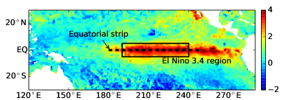
Figure 15: El Niño 3.4 region (rectangle) and the small strip around the equator used for the analysis in this work (dashed line). Color coding represents daily SST anomaly (in $\text{\,}\mathrm{\SIUnitSymbolDegree}\mathrm{C}$) on November 11, 2015.

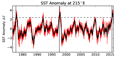
Figure 16: Exemplary time series of the SST anomaly at $215\text{\,}\mathrm{\SIUnitSymbolDegree}\mathrm{E}$ before (red) and after (black) Gaussian smoothing. The horizontal dashed line corresponds to a temperature threshold of $\Delta T_{\text{th}}=$2.5\text{\,}\mathrm{\SIUnitSymbolDegree}\mathrm{C}$$ used for event detection and the vertical lines are the resulting events identified from upward threshold crossings of the smoothed time series.

Starting from the smoothed SST profiles, we performed an event detection by identifying the onset of the SST anomaly connected with an El Niño in terms of an upward crossing of the smoothed time series with a temperature anomaly threshold $\Delta T_{\text{th}}$. As we are interested in the initial propagation front for each El Niño event, we additionally introduce an artificial refractory period of 11 months, which means threshold crossings occurring within 11 months after previous event are disregarded. Fig. 16 depicts this procedure for a threshold value $\Delta T_{\text{th}}=$2.5\text{\,}\mathrm{\SIUnitSymbolDegree}\mathrm{C}$$ leading to the identification of three events in this example (vertical lines in Fig. 16). From this, we finally arrive at $N=140$ discrete event series corresponding to the onsets of El Niño SST anomaly elevations at the different longitudinal locations along the dashed line in Fig. 15. The resulting spike trains are depicted in Fig. 17 on the left for four different threshold values $\Delta T_{\text{th}}=$1.5\text{\,}\mathrm{\SIUnitSymbolDegree}\mathrm{C}$\dots$3.0\text{\,}\mathrm{\SIUnitSymbolDegree}\mathrm{C}$$ (step size of $0.5$). The first thing to note is that this event detection procedure is able to correctly identify the El Niño occurrences as seen from the horizontal event structure in accordance with the El Niño years (labeled on the $x$-axis in the raster plots a-d) as well as the consistently high SPIKE-Synchronization values $C$ for all threshold values. With increasing temperature threshold, however, only the three strongest El Niño events are being captured (1983, 1998 and 2016, bold labels in Fig. 17) as seen from Fig. 17c and Fig. 17d.

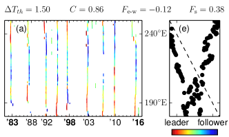
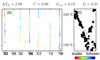
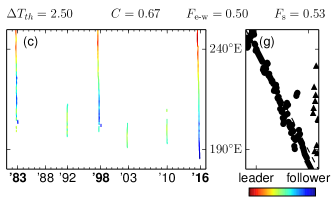
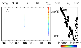
Figure 17: Spike Train Order analysis for propagation pattern of daily sea surface temperature anomalies within the equatorial strip ($$0.5\text{\,}\mathrm{\SIUnitSymbolDegree}\mathrm{S}$\dots$0.5\text{\,}\mathrm{\SIUnitSymbolDegree}\mathrm{N}$$, $$170\text{\,}\mathrm{\SIUnitSymbolDegree}\mathrm{E}$\dots$250\text{\,}\mathrm{\SIUnitSymbolDegree}\mathrm{E}$$) smoothed in time using a Gaussian kernel with width of $2\,\text{weeks}$. Events are defined as initial threshold crossings of the smoothed temperature time series (see text). From top to bottom four different threshold values have been used: $\Delta T_{\text{th}}=$1.5\text{\,}\mathrm{\SIUnitSymbolDegree}\mathrm{C}$\dots$3.0\text{\,}\mathrm{\SIUnitSymbolDegree}\mathrm{C}$$. The left graphs (a-d) show the event raster plots with with SPIKE-Order value in color coding using an east-to-west ordering. The years shown on the $x$-axis (representing January 1st of the indicated year) denote the moderate and strong (bold face) El Niño events. On the right (e-h), the optimal leader-follower order compared to an initial east-to-west sorting is shown (circles: spike trains with at least 2 spikes, triangles: spike trains with less than two spikes). Additionally, the SPIKE-Synchronization $C$ as well as the Synfire Indicator for the original (east-to-west) $F_{\text{e-w}}$, and the optimal sorting $F_{\text{s}}$ are reported.

To quantify the consistency of the propagation patterns, we perform a Spike Train Order analysis on these event sequences. The results are also presented in Fig. 17. As a central observation, we found that for the three strong El Niño events (1983, 1998, 2016), there is a clear consistent propagation of the SST anomaly elevation at the equator from east to west as confirmed by a Synfire Indicator of $F_{\text{e-w}}=0.5$ for the east-to-west sorting ($\Delta T_{\text{th}}=$2.5\text{\,}\mathrm{\SIUnitSymbolDegree}\mathrm{C}$$, Fig. Fig. 17c). Furthermore, optimizing the Synfire Indicator by changing the sorting only leads to minor improvements ($F_{\text{s}}=0.53$) and the resulting optimal order is very close to the original east-to-west sorting indicated in Fig. 17g. Finally, this observation is also confirmed by the SPIKE-Order based color coding in the raster plots (c) of the spike trains. For each of the three major El Niño events (1983, 1998, 2016) we see a clear tendency of leader (red) to follower (blue) going from east (top) to west (bottom) for all three threshold values. Further increase of the threshold temperature (Fig. 17d and h) leads to essentially the same observation, but parts of the longitudinal propagation might be missed as the SST anomaly maxima stay below threshold.

Moderate El Niño events (1992, 2003, 2010), on the other hand, seem to propagate in eastwards direction, as seen by opposite directed coloring for those years in Fig. 17b ($\Delta T_{\text{th}}=2.0$). Consequently, the Synfire Indicator for the east-to-west sorting is very low, $F_{\text{e-w}}=0.12$, as some of the propagation events are moving in the opposite direction which reduces the Synfire Indicator. Therefore, it is also not possible to find a correct ordering, as indicated by a rather low optimized Synfire Indicator of $F_{\text{s}}=0.31$ in this case. This is even more pronounced for the smallest threshold temperature $\Delta T_{\text{th}}=1.5$, shown in Fig. 17b. There, essentially all moderate El Niños are captured and most of those exhibit an eastwards propagation, opposed to the strong El Niños that propagate westwards. Therefore, the initial Synfire Indicator for the east-to-west sorting is negative, $F_{\text{e-w}}=-0.11$ and the optimal sorting shows the sign of a west-to-east propagation (Fig. 17e) with $F_{\text{s}}=0.38$.

To better understand the dependency of the Spike Train Order analysis on the temperature threshold, we computed the Synfire Indicator for the initial east-to-west ordering as well as the value for optimal ordering $F_{\text{s}}$ for varying thresholds $\Delta T_{\text{th}}=1.5\dots 3.5$ (Fig. 18). Additionally, Fig. 18 also shows the SPIKE-Synchronization values for these parameters. One first observes that the SPIKE-Synchronization remains rather constant over the whole range of threshold values, indicating a consistently good identification of the El Niño events. The Synfire Indicator for the original east-to-west sorting $F_{\text{e-w}}$ on the other hand shows a clear increase saturating in a plateau for a threshold value of around $\Delta T_{\text{th}}=$2.5\text{\,}\mathrm{\SIUnitSymbolDegree}\mathrm{C}$$, where it is then also very close to the optimal value $F_{\text{s}}$. This is easily understood by the fact that at temperature thresholds above $2.5\text{\,}\mathrm{\SIUnitSymbolDegree}\mathrm{C}$, only the three strong El Niños are captured that show a consistent westwards propagation, while for values below also weaker El Niños that exhibit eastward propagation enter the analysis.

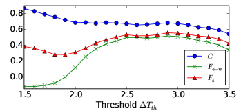
Figure 18: SPIKE-Synchronization $C$ and Synfire Indicator for the original sorting (east-to-west) $F_{\text{e-w}}$ and the optimal sorting $F_{\text{s}}$ in dependence of the temperature threshold $\Delta T_{\text{th}}$.

In summary, we showed that the newly proposed Spike Train Order method is also readily applicable to climate data and is able to identify propagation patterns in recurring events such as the El Niño. Our results indicate that close to the equator, strong El Niño events exhibit a clear westward propagation of an SST front, while for moderate El Niños we found indications for an eastward front propagation. Interestingly, previous results based on zonal current velocity within the El Niño 3.4 region found eastward propagation for the extreme El Niño events in 1983 and 1998 (Santoso et al. , 2013), while here we found west-ward propagation (Fig. 17). This discrepancy is most likely due to the different regions (El Niño 3.4 vs equatorial strip) and methodology (average warming/cooling rates vs front propagation).

4 Discussion

Over the last years a wide variety of measures to quantify the synchrony between spike trains have been introduced. Three recent proposals, ISI-distance (Kreuz et al. , 2007b, 2009), SPIKE-distance (Kreuz et al. , 2011, 2013), and SPIKE-Synchronization (Kreuz et al. , 2015; Mulansky et al. , 2015), share the desirable property of being time-resolved and parameter-free (time-scale independent). However, their bivariate versions are symmetric and in consequence their multivariate versions are invariant to changes in the order of spike trains. None of these measures is designed to provide information about the directionality of the propagation patterns.

In the present study we address this issue. First we use an adaptive coincidence detection as match maker in order to identify pairs of coincident spikes. Then we define two measures, the asymmetric SPIKE-Order $D$ and the symmetric Spike Train Order $E$, which are particularly useful in a bivariate representation (pairwise matrix) and as a time-resolved multivariate profile, respectively. From these two measures we can derive the Synfire Indicator $F$, a condensed scalar value that quantifies the overall consistency of the spatio-temporal propagation patterns in a rigorous and automated way. Its maximization allows to sort multiple spike trains from leader to follower. This is meant purely in the sense of temporal sequence of the spikes. The question asked is: For which spike trains do spikes tend to occur first and for which do they tend to occur last? We use simulated annealing to search among all permutations of spike trains for the sorting that resembles as closely as possible a synfire pattern, a perfectly consistent repetition of the same global propagation pattern. In a final step we evaluate the statistical significance of the optimized permutation using a set of carefully constructed spike train surrogates.

We first illustrate the merits of our new approach using artificially generated datasets and then apply it to real datasets from two very different fields of research, neuroscience and climatology. In the neurophysiological dataset we analyze Giant Depolarized Potentials (GDPs) recorded from mice brain slices in order to search for potential hub neurons (Bonifazi et al. , 2009), whereas in the climate application we quantify the consistency of the longitudinal movement of the propagation front of El Niño events (Santoso et al. , 2013).

The new algorithm is conceptually simple, of low computational cost and comes with an intuitive and straightforward visualization, including a color-coded rasterplot. It substantially improves on all the bivariate functionalities of its predecessor directional measure delay asymmetry (no need for sampled profiles, more intuitive normalization etc.) and could thus also be used in the context of the pairwise matrices, both normalized or cumulative, used in complex network theory (Malik et al. , 2010; Boers et al. , 2014). However, one of the main advantages of the new algorithm is its multivariate nature which opens up completely new kinds of application such as spike train sorting.

One important advantage that the method shares with other techniques of spike train analysis is the high flexibility in the definition of events. For example, when looking at the synchronization of neuronal bursts instead of individual spikes one can define the events as the onset, the center or the offset of the activity (e.g., the first, the middle or the last spike of each burst). In cases in which a burst of spikes is considered to be equivalent to a single spike one could introduce some kind of meta-events and then look at coincidences between these meta-events.

The application of our measures is also not restricted to truly discrete data. Continuously sampled data can be reduced to a spike train where the only information maintained is the timing of the individual events. Often these event times are obtained in a manner similar to how the neuronal spike times are extracted from recordings of neuronal membrane potentials (usually done via some kind of thresholding). Examples of sampled data to which measures of spike train synchrony have been applied include EEG data (Quian Quiroga et al. , 2002; Kreuz et al. , 2013; Rosário et al. , 2015) and, outside of neuroscience, stock market velocity (Zhou and Sornette , 2003) - and rainfall events (Malik et al. , 2010).

The algorithm is particularly suited for datasets with a high value of SPIKE-Synchronization. According to the coincidence criterion (Eq. 1) these are spike trains that include sequences of global events for which the interval between successive events is at least twice as large as the propagation time within an event. For these datasets the Synfire Indicator evaluates the consistency of the order within these well separated global events. The universality of the phenomenon, repetitive propagation patterns, makes our new algorithm applicable in a wide array of fields such as medical sciences, seismology, oceanography, meteorology or climatology. For example, the duration of an epileptic seizure is typically much shorter than the interval between two successive seizures. Also the time it takes a storm front to cross a specific region is typically much smaller than the time to the next storm. Many other repetitive propagation phenomena exhibit similar ratios of characteristic time scales.

In order to understand the scope of our proposed algorithm it is important to understand what it is not designed to achieve. The method deals purely with relative order, it does not consider the length of absolute delays. Moreover, while the instantaneous coincidence criterion makes the method time-scale independent, parameter-free and easy to use, it also renders it insensitive to patterns involving spikes that are not immediately adjacent. Many other, typically more complicated, methods have been designed to characterize the detailed spatio-temporal structure in large neuronal networks (Schneider et al. , 2006; Gansel and Singer, 2012) or to detect hierarchically structured spike-train communities (Billeh et al. , 2014; Russo and Durstewitz, 2017). The method is also not designed to detect neuronal synfire chains (in the strict sense of the word) in massively parallel data. For this task other statistical methods based on some forms of pattern detection have been developed (Schrader et al. , 2008; Gerstein et al. , 2012).

Another caveat concerns causality. While a significant value of the Synfire Indicator $F_{s}$ in our algorithm clearly shows the presence of a preferred temporal order of some signals with respect to others, it does not necessarily prove a driver-responder relationship. There are other methods that have been developed for this kind of system dynamics analysis (e.g., Andrzejak and Kreuz (2011)). But even for such methods causality is always a strong claim. In fact, the two signals might be driven by a common hidden source and a consistent leader (follower) could just indicate a drive with a smaller (larger) delay. Similarly, internal delay loops in one of the two systems can also fool the interpretation.

There are a number of possible directions for future research, both from a methods and from a data point of view. Regarding the algorithm, for the coincidence detection it would be straightforward to limit the range of allowed time lags by incorporating information about the expected speed of propagation (Malik et al. , 2010). One could introduce a minimum time lag in order to ensure causality and/or limit the maximally allowed time lag in order to focus on meaningful propagation of activity. In principle the range of allowed time lags could even be selected individually for each pair of spike trains depending on the known properties of the connectivity between the respective two neurons. Importantly, even with such type of time lag restrictions in place, it has still to be guaranteed that each spike can be part of at most one coincidence.

A follow-up task for our neurophysiological data would be to investigate to what extent the neurons that are identified as leading by our analysis are identical to the so-called hub neurons (Bonifazi et al. , 2009), i.e. neurons with a much higher than average degree of connectivity within the network. Regarding the El Niño analysis, the difference in propagation directions observed for the strong and weak El Niño events remains an open question. Furthermore, expanding the analysis to wider regions, i.e. $$5\text{\,}\mathrm{\SIUnitSymbolDegree}\mathrm{S}$\dots$5\text{\,}\mathrm{\SIUnitSymbolDegree}\mathrm{N}$$ and verifying the consistency of the observed propagation patterns is an interesting topic for future research. Finally, the relation to results based on average warming/cooling rates (Santoso et al. , 2013) requires further investigations.

The algorithm will be readily applicable for everyone since, together with the existing symmetric measures ISI-distance, SPIKE-distance, and SPIKE-Synchronization, SPIKE-Order is implemented in in three publicly available software packages, the Matlab-based graphical user interface SPIKY  (Kreuz et al. , 2015), cSPIKE  (Matlab command line with MEX-files), and the Python library PySpike  (Mulansky et al. , 2016).

Appendix A Neurophysiological dataset

The neurophysiological data analyzed in Section 3.2 were recorded via fast multicellular calcium imaging in acute CA3 hippocampal slices from juvenile mice. The CA3 region has a strong recurrent excitatory connectivity (Amaral and Witter, 1995). This distinct feature is suggested to be crucial for memory encoding and pattern completion and thus memory retrieval (Leutgeb and Leutgeb, 2007). During memory retrieval in rodents, population bursts of the CA3 lead to high frequency stimulation of the efferent regions, so called sharp wave ripples (Chrobak and Buzsáki, 1996). In the juvenile hippocampus, due to a higher chloride reversal potential in the CA3 pyramidal cells, the GABA-ergic system is excitatory (Ben-Ari et al. , 1989). GABA-ergic interneurons have been shown to serve as so called hub neurons that trigger the GDPs (Bonifazi et al. , 2009).

The recordings were performed by the group of Heinz Beck at the Department of Epileptology, University of Bonn, Germany, prior to and independently from the design of this study. Transversal acute brain slices ($300\mu m$ thick) were prepared from $5$ to $10$-day-old (P5-P10) C57BL/6 mice (Charles River, n = $19$ slices). Slice preparation, calcium imaging and data analysis were performed as previously described in (Hedrich et al. , 2014). For AM-loading of brain slices with OGB1-AM we used a protocol modified from (Crépel et al. , 2007). Multicellular calcium imaging was done using a homemade single planar illumination microscope (SPIM) modified from (Holekamp et al. , 2008). Movies were recorded at a frame rate of $200$ Hz over a minimal length of $5$ min up to $30$ min to record a sufficient amount of spontaneous activity. Time points of cell activity from the imaging data were defined as the onsets of Ca² events in fluorescence traces of all individual cells using the maximum of the second derivative of each event (Henze et al. , 2000).

In order to test the Spike Train Order algorithm, datasets were chosen that exhibited at least three global GDPs during the recording ($n=5$). For one dataset the surrogate analysis described in Section 2.5 proved to be unfeasible due to its excessive density of spontaneous activity. Therefore this dataset was discarded from further analysis, so the final number of datasets analyzed was $n=4$.

Appendix B El Niño dataset

The data analyzed in Section 3.3 describe one of the most well-known global climate effects, the so called El Niño, the warm phase of the El Niño Southern Oscillation (ENSO). It is usually characterized by an increased sea surface temperature (SST) in the central and eastern tropical Pacific Ocean typically during the months September – February (Trenberth , 1997). According to the U.S. National Oceanic and Atmospheric Administration (NOAA), an El Niño event is identified by an increased three-month moving average SST by $0.5\text{\,}\mathrm{\SIUnitSymbolCelsius}$ over at least six months. El Niños can last from nine months up to two years and typically occur in irregular intervals of two to seven years.

The analysis presented in Section 3.3 uses the Optimum Interpolated Sea Surface Temperature (OISST) data provided by NOAA. These data result from a high-resolution blended analysis (spatial resolution of $0.25\text{\,}\mathrm{\SIUnitSymbolDegree}$) of daily SST and ice constructed by combining observations from different platforms (satellites, ships, buoys) on a regular global grid with a time range from 1981 to 2016 (Reynolds et al. , 2007). The daily SST data is centralized by the long-term daily mean resulting in daily SST anomaly data (deviations from long-term mean) that form the basis of this analysis.

The area used to define El Niño events, the El Niño 3.4 region, stretches from $$5\text{\,}\mathrm{\SIUnitSymbolDegree}\mathrm{S}$\dots$5\text{\,}\mathrm{\SIUnitSymbolDegree}\mathrm{N}$$ in latitude and $$190\text{\,}\mathrm{\SIUnitSymbolDegree}\mathrm{E}$\dots$240\text{\,}\mathrm{\SIUnitSymbolDegree}\mathrm{E}$$ in longitude, as shown in Fig. 15. However, for the latitudinal direction we here focused only on a small central strip around the equator, i.e. from $$0.5\text{\,}\mathrm{\SIUnitSymbolDegree}\mathrm{S}$\dots$0.5\text{\,}\mathrm{\SIUnitSymbolDegree}\mathrm{N}$$ over a longitudinal stretch consistent with the El Niño region, i.e. from $$180\text{\,}\mathrm{\SIUnitSymbolDegree}\mathrm{E}$\dots$250\text{\,}\mathrm{\SIUnitSymbolDegree}\mathrm{E}$$ (dashed line in Fig. 15). Note, that this focus on the small region around the equator is the main difference to most previous works that studied the propagation of SST anomalies averaged over a much larger latitudinal extent, e.g. $$5\text{\,}\mathrm{\SIUnitSymbolDegree}\mathrm{S}$\dots$5\text{\,}\mathrm{\SIUnitSymbolDegree}\mathrm{N}$$ in Santoso et al. (2013); Antico and Barros (2016). In latitudinal direction, we average over the whole strip (four grid points), while in longitudinal direction an averaging over two grid points is performed resulting in $0.5\text{\,}\mathrm{\SIUnitSymbolDegree}$ of spatial resolution and a total of $N=140$ time series of daily SST anomalies. We disregard short-term fluctuation by applying a Gaussian smoothing with width $\sigma=$14\text{\,}\mathrm{d}\mathrm{a}\mathrm{y}\mathrm{s}$$. In Fig. 16 we show the time series resulting from this procedure exemplarily for the center of the observed region, $215\text{\,}\mathrm{\SIUnitSymbolDegree}\mathrm{E}$.

For the Sea Surface Temperature data we use a threshold criterion to identify the moving high temperature fronts of the El Niño events. The threshold determines the signal-to-noise ratio of the data: for small values even weaker events have an effect on the result, whereas for higher values the analysis is focused on the strongest El Niño events only. Due to the variability of the propagation patterns it might happen that in successive years the threshold is surpassed in different regions. However, since the aim of the analysis is to look at the propagation of individual (seasonal) fronts we suppress coincidences between threshold crossings from different years. We still use the adaptive coincidence detection from Eq. 1 but define a maximum coincidence window $\tau_{max}$ which in this case is set to $9$ months.

Acknowledgements We are indebted to Heinz Beck from the Department of Epileptology, University of Bonn, Germany, for providing the neurophysiological data. We thank Markus Abel, Roman Bauer, Heinz Beck, Nebojsa Bozanic, Christoph Gebhardt, Marcus Kaiser, Stefano Luccioli, Florian Mormann, Giorgia Paratore, and Alessandro Torcini for useful discussions. Finally, we are grateful to Irene Malvestio and Bernd Mulansky for carefully reading the manuscript. TK thanks Marcus Kaiser and his group for hosting him at the University of Newcastle, UK.

We acknowledge funding support from the European Commission through the Marie Curie Initial Training Network ‘Neural Engineering Transformative Technologies (NETT)’, project 289146 (TK and MM), and through the European Joint Doctorate ‘Complex oscillatory systems: Modeling and Analysis (COSMOS)’, project 642563 (TK and ES). TK also acknowledges the Italian Ministry of Foreign Affairs regarding the activity of the Joint Italian-Israeli Laboratory on Neuroscience.

References

- Abeles (2009) Abeles, M., Synfire chains. Scholarpedia 4 (7), 1441 (2009).
- Amaral and Witter (1995) Amaral, D. G., Witter, M. P., Hippocampal formation, Paxinos G., The rat nervous system, 443-493 (1995).
- An and Wang (2000) An, S. I., Wang, B., Interdecadal change of the structure of the ENSO mode and its impact on the ENSO frequency. J Climate 13 (12), 2044-2055 (2000).
- Andrzejak and Kreuz (2011) Andrzejak, R. G., Kreuz, T., Characterizing unidirectional couplings between point processes and flows. Europhysics Letters 96, 50012 (2011).
- Antico and Barros (2016) Antico, P. L., Barros, V. R., Changes in the zonal propagation of El Niño-related SST anomalies: A possible link to the PDO. Theoretical and Applied Climatology, 1-6 (2016).
- Applegate et al. (2011) Applegate, D. L., Bixby, R. E., Chvatal, V., Cook, W. J., The traveling salesman problem: A computational study. Princeton University Press (2011).
- Baier et al. (2012) Baier, G., Goodfellow, M., Taylor, P. N., Wang, Y., Garry, D. J., The importance of modeling epileptic seizure dynamics as spatio-temporal patterns. Front Physiol 3, 281 (2012).
- Belik et al. (2011) Belik, V., Geisel, T., Brockmann, D., Natural human mobility patterns and spatial spread of infectious diseases. Physical Review X 1 (1), 011001 (2011).
- Ben-Ari et al. (1989) Ben‐Ari, Y., Cherubini, E., Corradetti, R., Gaiarsa, J. L., Giant synaptic potentials in immature rat CA3 hippocampal neurones. J Physiol 416 (1), 303-325 (1989).
- Billeh et al. (2014) Billeh, Y. N., Schaub, M. T., Anastassiou, C. A., Barahona, M., Koch, C., Revealing cell assemblies at multiple levels of granularity. J Neurosci Methods 236, 92-106 (2014).
- Boccaletti et al. (2014) Boccaletti, S., Bianconi, G., Criado, R., Del Genio, C. I., Gómez-Gardenes, J., Romance, M., Sendiña-Nadal, I., Wang, Z., Zanin, M, The structure and dynamics of multilayer networks. Physics Reports 544 (1), 1-122 (2014).
- Boers et al. (2014) Boers, N., Bookhagen, B., Barbosa, H. M. J., Marwan, N., Kurths, J., Marengo, J. A., Prediction of extreme floods in the eastern central andes based on a complex networks approach. Nature Communications 5, 5199 (2014).
- Bonifazi et al. (2009) Bonifazi P., Goldin M., Picardo, M. A., Jorquera, I., Cattani, A., Bianconi, G., Represa, A., Ben-Ari, Y., Cossart, R., Gabaergic hub neurons orchestrate synchrony in developing hippocampal networks. Science 326, 1419 (2009).
- Chrobak and Buzsáki (1996) Chrobak, J. J., Buzsáki, G., 1996. High-frequency oscillations in the output networks of the hippocampal–entorhinal axis of the freely behaving rat. Journal of neuroscience 16 (9), 3056–3066.
- Crépel et al. (2007) Crépel, V., Aronov, D., Jorquera, I., Represa, A., Ben-Ari, Y., Cossart, R., 2007. A parturition-associated nonsynaptic coherent activity pattern in the developing hippocampus. Neuron 54, 105.
- Dowsland and Thompson (2012) Dowsland, K. A., Thompson, J. M., 2012. Simulated annealing. In: Handbook of Natural Computing. Springer, pp. 1623-1655.
- Earl and Deem (2005) Earl, D. J., Deem, M. W., 2005. Parallel tempering: Theory, applications, and new perspectives. Physical Chemistry Chemical Physics 7 (23), 3910-3916.
- Gallos et al. (2012) Gallos, L. K., Rybski, D., Liljeros, F., Havlin, S., Makse, H. A., 2012. How people interact in evolving online affiliation networks. Physical Review X 2 (3), 031014.
- Gansel and Singer (2012) Gansel, K. S., Singer, W., 2012. Detecting multineuronal temporal patterns in parallel spike trains. Frontiers in Neuroinformatics 6, 18.
- Gerstein et al. (2012) Gerstein, G. L., Williams, E. R., Diesmann, M., Grün, S., Trengove, C., 2012. Detecting synfire chains in parallel spike data. J Neurosci Methods 206 (1), 54-64.
- Hedrich et al. (2014) Hedrich, U. B., Liautard, C., Kirschenbaum, D., Pofahl, M., Lavigne, J., Liu, Y., Theiss, S., Slotta, J., Escayg, A., Dihné, M., et al., 2014. Impaired action potential initiation in GABAergic interneurons causes hyperexcitable networks in an epileptic mouse model carrying a human NaV1. 1 mutation. J Neurosci 34 (45), 14874.
- Heidemann et al. (2012) Heidemann, J., Stojanovic, M., Zorzi, M., 2012. Underwater sensor networks: applications, advances and challenges. Philosophical Transactions of the Royal Society of London A: Mathematical, Physical and Engineering Sciences 370 (1958), 158-175.
- Henze et al. (2000) Henze, D. A., González-Burgos, G. R., Urban, N. N., Lewis, D. A., Barrionuevo, G., 2000. Dopamine increases excitability of pyramidal neurons in primate prefrontal cortex. J Neurophysiol 84, 2799.
- Holekamp et al. (2008) Holekamp, T. F., Turaga, D., Holy, T. E., 2008. Fast three-dimensional fluorescence imaging of activity in neural populations by objective-coupled planar illumination microscopy. Neuron 57, 661.
- Kistler et al. (1997) Kistler, W. M., Gerstner, W., Leo van Hemmen, J., 1997. Reduction of Hodgkin-Huxley equations to a single variable threshold model. Neural Comput 9, 1015.
- Kreuz et al. (2007a) Kreuz, T., Mormann, F., Andrzejak, R. G., Kraskov, A., Lehnertz, K., Grassberger, P., 2007a. Measuring synchronization in coupled model systems: A comparison of different approaches. Phys D 225, 29.
- Kreuz et al. (2007b) Kreuz, T., Haas, J. S., Morelli, A., Abarbanel, H. D. I., Politi, A., 2007b. Measuring spike train synchrony. J Neurosci Methods 165, 151.
- Kreuz et al. (2009) Kreuz, T., Chicharro, D., Andrzejak, R. G., Haas, J. S., Abarbanel, H. D. I., 2009. Measuring multiple spike train synchrony. J Neurosci Methods 183, 287.
- Kreuz et al. (2011) Kreuz, T., Chicharro, D., Greschner, M., Andrzejak, R. G., 2011. Time-resolved and time-scale adaptive measures of spike train synchrony. J Neurosci Methods 195, 92.
- Kreuz et al. (2013) Kreuz, T., Chicharro, D., Houghton, C., Andrzejak, R. G., Mormann, F., 2013. Monitoring spike train synchrony. J Neurophysiol 109, 1457.
- Kreuz et al. (2015) Kreuz, T., Mulansky, M., Bozanic, N., 2015. SPIKY: A graphical user interface for monitoring spike train synchrony. J Neurophysiol 113, 3432.
- Kuhn et al. (2014) Kuhn, T., Perc, M., Helbing, D., 2014. Inheritance patterns in citation networks reveal scientific memes. Physical Review X 4 (4), 041036.
- Kuramoto (2012) Kuramoto, Y., 2012. Chemical oscillations, waves, and turbulence. Vol. 19. Springer Science & Business Media.
- Lacroix et al. (2012) Lacroix, P., Grasso, J.-R., Roulle, J., Giraud, G., Goetz, D., Morin, S., Helmstetter, A., 2012. Monitoring of snow avalanches using a seismic array: Location, speed estimation, and relationships to meteorological variables. J Geophys Research: Earth Surface 117 (F1).
- Lazer et al. (2009) Lazer, D., Pentland, A. S., Adamic, L., Aral, S., Barabasi, A. L., Brewer, D., Christakis, N., Contractor, N., Fowler, J., Gutmann, M., et al., 2009. Life in the network: the coming age of computational social science. Science (New York, NY) 323 (5915), 721.
- Leutgeb and Leutgeb (2007) Leutgeb, S., Leutgeb, J. K., 2007. Pattern separation, pattern completion, and new neuronal codes within a continuous ca3 map. Learning & memory 14 (11), 745–757.
- Lewis et al. (2015) Lewis, C., Bosman, C., Fries, P., 2015. Recording of brain activity across spatial scales. Current Opinion in Neurobiology 32, 68-77.
- Malik et al. (2010) Malik, N., Marwan, N., Kurths, J., 2010. Spatial structures and directionalities in monsoonal precipitation over south asia. Nonlinear Process Geophys 17, 371.
- Malik et al. (2012) Malik, N., Bookhagen, B., Marwan, N., Kurths, J., 2012. Analysis of spatial and temporal extreme monsoonal rainfall over south asia using complex networks. Climate Dynamics 39 (3-4), 971-987.
- Maranò et al. (2014) Maranò, S., Fäh, D., Lu, Y. M., 2014. Sensor placement for the analysis of seismic surface waves: sources of error, design criterion and array design algorithms. Geophys J International, ggt489.
- McPhaden et al. (2006) McPhaden, M. J., Zebiak, S. E., Glantz, M. H., 2006. ENSO as an integrating concept in earth science. Science 314 (5806), 1740-1745.
- Menne et al. (2012) Menne, M. J., Durre, I., Vose, R. S., Gleason, B. E., Houston, T. G., 2012. An overview of the global historical climatology network-daily database. J Atmospheric and Oceanic Technology 29 (7), 897-910.
- Mulansky et al. (2015) Mulansky, M., Bozanic, N., Sburlea, A., Kreuz, T., 2015. A guide to time-resolved and parameter-free measures of spike train synchrony. Event-based Control, Communication, and Signal Processing (EBCCSP) International Conference on, 1-8.
- Mulansky et al. (2016) Mulansky, M., Kreuz, T., 2016. PySpike - a Python library for analyzing spike train synchrony. Software X (in press).
- Muller et al. (2013) Muller, C. L., Chapman, L., Grimmond, C., Young, D. T., Cai, X., 2013. Sensors and the city: A review of urban meteorological networks. International J Climatology 33 (7), 1585-1600.
- Naud et al. (2011) Naud, R., Gerhard, F., Mensi, S., Gerstner, W., 2011. Improved similarity measures for small sets of spike trains. Neural Comput 23, 3016.
- Pelinovsky et al. (2006) Pelinovsky, E., 2006. Waves in Geophysical Fluids: Tsunamis, Rogue Waves, Internal Waves and Internal Tides. Springer Vienna, Vienna, Ch. Hydrodynamics of Tsunami Waves, pp. 1-48.
- Pereda et al. (2005) Pereda, E., Quian Quiroga, R., Bhattacharya, J., 2005. Nonlinear multivariate analysis of neurophysiological signals. Progress in Neurobiology 77, 1.
- Qian et al. (2011) Qian, C., Wu, Z., Fu, C., Wang, D., 2011. On changing El Niño: A view from time-varying annual cycle, interannual variability, and mean state. J Climate 24 (24), 6486-6500.
- Quian Quiroga et al. (2002) Quian Quiroga, R., Kreuz, T., Grassberger, P., 2002. Event synchronization: A simple and fast method to measure synchronicity and time delay patterns. Phys. Rev. E 66, 041904.
- Rahbar et al. (2015) Rahbar, F., Anzalone, S., Varni, G., Zibetti, E., Ivaldi, S., Chetouani, M., 2015. Predicting extraversion from nonverbal features during a face-to-face human-robot interaction. International Conference on Social Robotics, 10.
- Rasmusson et al. (1982) Rasmusson, E. M., Carpenter, T. H., 1982. Variations in tropical sea surface temperature and surface wind fields associated with the southern oscillation/El Niño. Monthly Weather Rev 110 (5), 354-384.
- Reynolds et al. (2007) Reynolds, R. W., Smith, T. M., Liu, C., Chelton, D. B., Casey, K. S., Schlax, M. G., 2007. Daily high-resolution-blended analyses for sea surface temperature. J Climate 20 (22), 5473-5496.
- Rieke et al. (1996) Rieke, F., Warland, D., de Ruyter van Steveninck, R., Bialek, W., 1996. Spikes: Exploring the neural code. Institute of Technology, Cambridge, Massachusetts.
- Rosário et al. (2015) Rosário, R. S., Cardoso, P. T., Muñoz, M. A., Montoya, P., Miranda, J. G. V., 2015. Motif-synchronization: A new method for analysis of dynamic brain networks with EEG. Physica A 439, 7.
- Russo and Durstewitz (2017) Russo, E., Durstewitz, D., 2017. Cell assemblies at multiple time scales with arbitrary lag constellations. eLife 6, e19428.
- Santoso et al. (2013) Santoso, A., McGregor, S., Jin, F.-F., Cai, W., England, M. H., An, S.-I., McPhaden, M. J., Guilyardi, E., 2013. Late-twentieth-century emergence of the El Niño propagation asymmetry and future projections. Nature 504 (7478), 126-130.
- Schneider et al. (2006) Schneider, G., Havenith, M. N., Nikolić, D., 2006. Spatiotemporal structure in large neuronal networks detected from cross-correlation. Neural Computation 18 (10), 2387-2413.
- Schrader et al. (2008) Schrader, S., Grün, S., Diesmann, M., Gerstein, G. L., 2008. Detecting synfire chain activity using massively parallel spike train recording. J Neurophysiol 100 (4), 2165-2176.
- Spira and Hai (2013) Spira, M. E., Hai, A., 2013. Multi-electrode array technologies for neuroscience and cardiology. Nature Nanotechnology 8 (2), 83-94.
- Takano et al. (2012) Takano, H., McCartney, M., Ortinski, P. I., Yue, C., Putt, M. E., Coulter, D. A., 2012. Deterministic and stochastic neuronal contributions to distinct synchronous CA3 network bursts. J Neurosci 32 (14), 4743-4754.
- Trenberth (1997) Trenberth, K. E., 1997. The definition of El Niño. Bulletin of the American Meteorological Society 78 (12), 2771-2777.
- Varni et al. (2010) Varni, G., Volpe, G., Camurri, A., 2010. A system for realtime multimodal analysis of nonverbal affective social interaction in user-centric media. IEEE Transactions on Multimedia 12, 576.
- Wei et al. (2013) Wei, X., Valler, N. C., Prakash, B. A., Neamtiu, I., Faloutsos, M., Faloutsos, C., 2013. Competing memes propagation on networks: A network science perspective. Selected Areas in Communications, IEEE Journal on 31 (6), 1049-1060.
- Yeh et al. (2009) Yeh, S.-W., Kug, J.-S., Dewitte, B., Kwon, M.-H., Kirtman, B. P., Jin, F.-F., 2009. El Niño in a changing climate. Nature 461 (7263), 511-514.
- Zhou and Sornette (2003) Zhou, W. X., Sornette, D. Evidence of a worldwide stock market log-periodic anti-bubble since mid-2000. Physica A: Statistical Mechanics and its Applications 330, 543 (2003).