3d ${\cal N}=2$ minimal SCFTs from Wrapped M5-branes

Abstract

We study CFT data of 3-dimensional superconformal field theories (SCFTs) arising from wrapped two M5-branes on closed hyperbolic 3-manifolds. Via so-called 3d/3d correspondence, central charges of these SCFTs are related to a $SL(2)$ Chern-Simons (CS) invariant on the 3-manifolds. We give a rigorous definition of the invariant in terms of resurgence theory and a state-integral model for the complex CS theory. We numerically evaluate the central charges for several closed 3-manifolds with small hyperbolic volume. The computation suggests that the wrapped M5-brane systems give infinitely many discrete SCFTs with small central charges. We also analyze these ‘minimal’ SCFTs in the eye of 3d ${\cal N}=2$ superconformal bootstrap.

1 Introduction and Conclusion

Quantum field theory (QFT) has become the dominant language in theoretical physics since the success of quantum electrodynamics. The usage of QFT is not restrict to particle physics but ubiquitous: statistical, condensed matter system and even quantum gravity using holography. In general, QFTs are in the form of

$$\textrm{QFT}\;:\;\textrm{(a CFT with flavor symmetry $G$)+(deformation)+(gauging $H\subset G$)}\;.$$

At infrared (IR) limit, a QFT flows to another conformal field theory (CFT). So, the general QFTs can be thought as RG flows between CFTs and thus understanding general CFTs is the first step toward understanding QFTs.

“ Classify consistent CFTs and solve them ”

One rigorous way of defining a CFT is specifying CFT data: spectrum of local operators $\{O_{I}\}$ and their operator product expansion (OPE) coefficients $\{\lambda_{IJK}\}$. By solving a CFT, we mean determining these CFT data.

In this work, we study 3d ${\cal N}=2$ unitary superconformal field theories (SCFTs) without any flavor symmetry and with small central charges. 3d supersymmetry has not been observed experimentally yet. But there is a concrete proposal for condensed matter system Ponte:2012ru ; Grover:2013rc which exhibits an emergent supersymmetry and described by a 3d SCFT called critical Wess-Zumino (cWZ) model. The model is known to be the simplest 3d ${\cal N}=2$ SCFT with smallest central charge $c_{T}/c_{T}^{free}=\frac{16}{243}\left(16-\frac{9\sqrt{3}}{\pi}\right)\simeq 0.7268$ Witczak-Krempa:2015jca where $c_{T}^{free}$ is the central charge for a free chiral theory. Classifying such simple unitary CFTs is an interesting open question. In two dimensional spacetime, there is a complete classification when $c_{T}<1$ called 2d minimal models. Here, we propose 3d ${\cal N}=2$ ‘minimal’ SCFTs based on wrapped M5-brane systems.

An efficient way of constructing 3d ${\cal N}=2$ SCFTs is using wrapped M5-branes system in M-theory:

$$11d\;\textrm{space-time : }\;\; \mathbb{R}^{1,2}\times T^{*}M\times\mathbb{R}^{2}\;$$

$$\;\;\;\;\;\;\;\bigcup$$ (1)

$$N\;M5\textrm{-branes}\;:\;\;\; \mathbb{R}^{1,2}\times M\;.$$

Here $T^{*}M$ denotes the cotangent bundle of $M$. The IR fixed point of the wrapped M5-branes’ world-volume theory defines a 3d ${\cal N}=2$ SCFT. It is labelled by an orientable closed hyperbolic 3-manifold (${\rm CH3}$) $M$ and an integer $N\geq 2$. We denote the SCFT as $T_{N}[M]$. The space of CH3 with small hyperbolic volume is depicted in Figure 1.

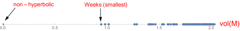
Figure 1: Space of closed 3-manifolds $M$ with $\textrm{vol}(M)<\textrm{vol}\big{(}(S^{3}\backslash{\bf 5^{2}_{1}})_{(5,-1)}\big{)}\simeq 2.02988$. ${\rm vol(M)}$ denotes a topological invariant of 3-manifold $M$ called hyperbolic volume, the volume measured in the unique hyperbolic metric $(R_{\mu\nu}=-2g_{\mu\nu})$. For each non-zero hyperbolic volume plotted in the graph, there are only finitely many (mostly unique) ${\rm CH3}$s. The spectrum is discrete and infinite and has a (non-zero) lower bound 0.9427 which is saturated by the Weeks manifold ($(S^{3}\backslash{\bf 5^{2}_{1}})_{(5,-1)(5,-2)}$) 2007arXiv0705.4325G .

For nomenclature of 3-manifolds, we use a Dehn surgery description (30) on $S^{3}$ along a White-head link in Figure 3. One natural question is

“ Solve $$T[M] M$$ for closed hyperbolic 3-manifolds ”. (2)

As a first step we develop a systematic algorithm for computing the central charge of wrapped M5-brane CFTs. The algorithm can be summarized as :

$$\big{(}\textrm{a surgery description \eqref{surgery description} of $M$ and an ideal triangulation \eqref{classical triangulation}}\big{)}\;,$$

$$\xRightarrow{\;\;\;\;\;\;\;}\big{(}\textrm{State-integral model in eq.~{}\eqref{quantum ideal triangulation} and \eqref{Dehns-filling}}\big{)}\;,$$

$$\xRightarrow{\;\;\;\;\;\;\;}\textrm{\big{(}Perturbative expansion $\{S_{n}^{\overline{\textrm{hyp}}}(M)\}_{n=0}^{\infty}$ in eq.~{}\eqref{def of S^{conj}}\big{)}}\;,$$

$$\xRightarrow{\;\;\;\;\;\;\;}\textrm{\big{(}Borel resummation to ${\cal Z}^{\overline{\textrm{hyp}}}(M;\hbar)$ in eq.~{}\eqref{Z^{conj} from borel sum}\big{)}}\;,$$ (3)

$$\xRightarrow{\;\;\;\;\;\;\;}\textrm{\big{(}${\cal Z}\big{[}\textrm{$T[M]$ on $S^{3}_{b}$}\big{]}$ using 3d/3d relation in eq.~{}\eqref{3d/3d in resurgence}\big{)}}\;,$$

$$\xRightarrow{\;\;\;\;\;\;\;}\textrm{\big{(}$c_{T}\big{(}T[M]\big{)}$ using the relation in eq.~{}\eqref{squashed free-energy and central charge}\big{)}}\;.$$

In the procedure, a) we reformulate the 3d/3d correspondence for squashed 3-sphere partition function (ptn) in the language of resurgence and b) develop a state-integral for $SL(2)$ Chern-Simons theory on closed hyperbolic 3-manifolds. We numerically evaluate the central charge for three examples listed in Table 1.

	Weeks: $(S^{3}\backslash{\bf 5^{2}_{1}})_{(5,-1)(5,-2)}$	Thurston: $(S^{3}\backslash{\bf 5^{2}_{1}})_{(5,-1)(1,-2)}$	$(S^{3}\backslash{\bf 5^{2}_{1}})_{(5,-1)(5,-1)}$
$c_{T}(T[M])$	0.93	1.01	1.28
vol($M$)	0.9427	0.9814	1.2637

Table 1: Central charge of $T[M]$ and hyperbolic volume for three CH3s.

From the three examples, we see that the central charge is well-approximated by the hyperbolic volume within a few percent error. With this observation on top of Weeks manifold having smallest non-zero hyperbolic volume, we expect that the $T[{\it Weeks}]$ to be the simplest non-trivial wrapped M5-brane SCFT and there are infinitely many discrete SCFTs with small central charge $(\lesssim 2)$.

In recent years, the conformal bootstrap has provided valuable insights in strongly-interacting CFTs in $d\geq 2$ spacetime dimensions started with pioneering work of Rattazzi:2008pe . Studying even a small subset of crossing symmetry constraints combined with unitarity was surprisingly restrictive on the allowed CFT data. The approach is quite universal and have been used to study CFTs in various spacetime dimensions with various number of supersymmetries and global symmetries ElShowk:2012ht ; El-Showk:2014dwa ; Kos:2013tga ; Nakayama:2014yia ; Poland:2010wg ; Poland:2011ey ; Beem:2013qxa ; Beem:2014zpa ; Beem:2015aoa ; Chester:2014fya ; Iliesiu:2015qra ; Lin:2015wcg ; Lin:2016gcl . It provides truly non-perturbative approach to probe full spaces of CFTs without reference to specific microscopic description, therefore providing another important tool for studying wrapped M5-brane CFTs.

For this purpose, we refer to the study for 3d ${\cal N}=2$ was initiated in Bobev:2015vsa ; Bobev:2015jxa . In the dimension bound for unprotected operator there exist a kink which is connected to the kink observed in 4d ${\cal N}=1$ superconformal bootstrap Poland:2011ey ; Poland:2015mta . It has been proposed that this kink might be signalling some unknown ‘minimal’ SCFT. In this work, we further analyze and improve upon the results of Bobev:2015vsa ; Bobev:2015jxa to make connections to wrapped M5-brane CFTs as possible candidates for the kink theory. Using chiral ring relation $\Phi^{2}\sim 0$ for chiral primary operator $\Phi$, our best estimate for the CFT data obtained using numerical superconformal bootstrap is $\Delta_{\Phi}\geq 0.87$, $c_{T}/c_{T}^{free}\geq 1.0361$ and $\Delta_{\bar{\Phi}\Phi}\leq 2.3624$.

This work put the first step toward the challenging problem (2) and there are several interesting directions worth exploring. We hope to report progresses on these in near future.
$\bullet$ Justify the physical and technical assumptions ((21) and (60)) used in the central charge computation. We give some circumstantial evidences for them.
$\bullet$ Prove topological invariance of the state-integral model developed in Section 3.1.1. The state-integral model is based on a Dehn surgery representation (30) of a 3-manifold. The representation is not unique and we need to show the independence on the choice. We check it perturbatively up to two-loops for several cases.
$\bullet$ Determine BPS operator spectrum of the $T[M]$. As noticed in Section 3.2, it is related to the problem of refinement/categorification of Chern-Simons invariants on CH3s.
$\bullet$ Using the central charge and BPS operator spectrum obtained above, bootstrap the $T[M]$ following Beem:2015aoa .

The paper is organized as follows. In Section 2, we introduce wrapped M5-brane SCFTs and their basic properties. We also present a rigorous form of 3d/3d relation for $S^{3}_{b}$-ptn in terms of resurgence theory. In Section 3, a systematic algorithm for computing the central charge is given. It is based on a state-integral for a complex CS theory developed in the section. We give explicit examples for the computation and comments on the difficulties in determining chiral operator spectrum. In Section 4, we investigate the possibility of SCFTs at kinks in numerical bootstrap being identified with wrapped M5-brane SCFTs.

2 Wrapped M5-brane SCFT and 3d/3d correspondence

We introduce a 3d SCFT $T[M]$ labelled by a closed 3-manifold $M$ and review basic aspects (holography and 3d/3d correspondence) of the SCFT. Especially, we reformulate the 3d/3d relation for squashed 3-sphere ptn in terms of resurgence theory. For recent studies on the topic, refer to Dimofte:2010tz ; Terashima:2011qi ; Terashima:2011xe ; Dimofte:2011jd ; Dimofte:2011ju ; Dimofte:2011py ; Dimofte:2013iv ; Gang:2013sqa ; Yagi:2013fda ; Lee:2013ida ; Cordova:2013cea ; Chung:2014qpa ; Dimofte:2014zga ; Gang:2014ema ; Gang:2015wya ; Pei:2015jsa (see also recent review Dimofte:2016pua ).

2.1 3d ${\cal N}=2$ SCFT $T_{N}[M]$

A 3d SCFT $T_{N}[M]$ is defined as an infrared (IR) fixed point of twisted compactification of 6d $A_{N-1}$ $(2,0)$ theory on a closed 3-manifold $M$:

6d $$A_{N-1} \mathbb{R}^{1,2}\times M M$$ (2,0) theory on with partial topological twisting along

$$\xrightarrow{\;\;\;\;\textrm{IR}\;\;\;}\;\;\textrm{3d SCFT $T_{N}[M]$}\;.$$ (4)

For the partial twisting, we use the usual $SO(3)$ subgroup of $SO(5)$ R-symmetry of the 6d theory. The twisting generically preserves a quarter of supercharges and the resulting 3d theory has ${\cal N}=2$ superconformal symmetry. The metric structure on the 3-manifold is irrelevant in the IR and the 3d SCFT depends only on the topology of the 3-manifold. From M-theoretical perspective, these theories are realized as low-energy world-volume theory of wrapped $N$ M5-branes in (1). As pointed out in Chung:2014qpa , the ‘full’ IR CFT has an additional abelian flavor symmetry called $U(1)_{t}$ and will be denoted as $T^{\rm full}_{N}[M]$.

	$T^{\textrm{full}}_{N}[M]$	$T_{N}[M]$
Global symmetry	$U(1)_{R}\times U(1)_{t}$	$U(1)^{\rm IR}_{R}$
3d/3d correspondence	“Refined” $SL(N)$ CS theory	$SL(N)$ CS theory
Large $N$ gravity dual	Unknown	$AdS_{4}\times M\times S^{4}$ (for $CH3$)

Table 2: Comparison between $T^{\rm full}_{N}[M]$ and $T_{N}[M]$.

The theory $T_{N}[M]$ of our interest is obtained as IR fixed point of the $T^{\rm full}_{N}[M]$ through a renormalization group (RG) flow triggered by a Higgsing/deformation procedure

$$\big{(}T^{\rm full}_{N}[M]+\textrm{ Higgsing/deformation}\big{)}\;\;\leadsto\;\;T_{N}[M]\;.$$ (5)

Not all 3-manifolds $M$ give non-trivial interacting CFTs. Our basic assumptions are

a) For hyperbolic 3-manifold $M$, the IR fixed theory $T_{N}[M]$ is non-trivial.

b) For non-hyperbolic 3-manifold $M$ with $SO(3)$ Riemmanian holonomy (for example, $M=S^{3}$), the corresponding $T_{N}[M]$ seems to be more or less trivial theories (theories only with topological degree of freedom).

c) $M$ has reduced Riemannina holonomy group (thus non-hyperbolic), i.e, $M=\Sigma\times S^{1}$ with a Riemann surface $\Sigma$. In the case, the resulting 3d SCFT has additional structure, enhanced ${\cal N}=4$ SUSY or additional flavor symmetry.

Simple evidence for a) is

$$\lim_{b\rightarrow 0}2\pi b^{2}{\cal F}_{b}(T_{N}[M])=\frac{N(N^{2}-1)}{6}\textrm{vol}(M)\;.$$ (6)

Here ${\cal F}_{b}$ denotes the free-energy on a squashed 3-sphere $S^{3}_{b}$ Hama:2011ea ,

$${\cal F}_{b}(\textrm{a SCFT}) :=(\textrm{free-energy of the SCFT on $S^{3}_{b}$})$$

$$:=-\textrm{Re}\big{(}\log{\cal Z}[\textrm{the SCFT on $S^{3}_{b}$}]\big{)}\;.$$ (7)

Metrically, the curved background can be realized as

$$S^{3}_{b}=\{b^{2}|z|^{2}+b^{-2}|w|^{2}=1\;:\;(z,w)\in\mathbb{C}^{2}\}\;,\quad\textrm{with real $b$}.$$ (8)

The geometry has an exact symmetry exchanging $b\leftrightarrow b^{-1}$ and so does the free-energy ${\cal F}_{b}$. The relation in eq. (6) can be explained using a 3d/3d relation and perturbative expansion of $SL(N)$ CS theory as we will see in the next section. Since we are interested in a non-trivial 3d ${\cal N}=2$ SCFT with small central charge and no extra structures (flavor symmetry or enhacencd SUSY), we concentrate on $N=2$ and the case a).

Holographic dual

Holographic dual to the RG flow (4) across dimension was constructed in Gauntlett:2000ng

$$(\;AdS_{7}\times S^{4}\;\textrm{solution}\;)\xrightarrow{\;\;\;\;\textrm{Holographic RG}\;\;\;}(\;\textrm{Pernici-Sezgin $AdS_{4}$ solution in }\;)$$

and M-theory on the $AdS_{4}$ solution is proposed as gravity dual of $T_{N}[M]$. The supergravity solution is

$$AdS_{4}\times M\times S^{4}\;,$$ (9)

with a warped product metric and the $S^{4}$ non-trivially fibred over the $M$ factor. The supergravity solution was found only for closed hyperbolic $M$. From the holographic computation using supergravity approximation, it has been predicted that Gang:2014ema

$$\lim_{N\rightarrow\infty}\frac{1}{N^{3}}{\cal F}_{b}(T_{N}[M])=\frac{(b+b^{-1})^{2}}{12\pi}\textrm{vol}(M)\;.$$ (10)

2.2 3d/3d relation and resurgence

Naively, 3d/3d relation relates the squashed 3-sphere ptn of $T_{N}[M]$ to ptn of $SL(N)$ CS theory on $M$.

$${\cal Z}[T_{N}[M]\textrm{ on }S^{3}_{b}]={\cal Z}\big{[}SL(N)_{k,\sigma}\textrm{ CS theory on }M\big{]}$$

$$:=\int\frac{[D{\cal A}]}{(\textrm{gauge})}\exp\bigg{(}\frac{i(k+\sigma)}{8\pi}\textrm{CS}[{\cal A}]+\frac{i(k-\sigma)}{8\pi}\textrm{CS}[\bar{{\cal A}}]\bigg{)}\;,$$ (11)

where $k$ and $\sigma$ are two coupling constants of the complex CS theory. $k\in\mathbb{Z}$ is a quantized CS level and the $\sigma$ can be either real or purely imaginary. In the 3d/3d relation for $S^{3}_{b}$-ptn, they are Cordova:2013cea ; Dimofte:2014zga

$$k=1\;\;\textrm{and}\;\;\sigma=\frac{1-b^{2}}{1+b^{2}}\;.$$ (12)

${\cal A},\bar{{\cal A}}$ denote a pair of $SL(N)$ gauge fields on $M$ and the CS functional is defined as

$$\textrm{CS}[{\cal A}]:=\int_{M}\textrm{Tr}\bigg{(}{\cal A}\wedge d{\cal A}+\frac{2}{3}{\cal A}\wedge{\cal A}\wedge{\cal A}\bigg{)}\;.$$ (13)

The path-integral on the complex CS theory is ambiguous since there is no canonical choice for the path-integral contour and gauge transformation for real $\sigma$. See sec 2.1 in Gang:2015wya for discussion on the issue.

Goal of this section is to make the 3d/3d relation more rigorous avoiding these ambiguities. For the purpose, we use the language of resurgence theory.

Perturbative ptn ${\cal Z}^{\overline{\textrm{hyp}}}_{N;\rm pert}$

When $b^{2}\rightarrow 0^{+}$, the $S^{3}_{b}$-ptn has following asymptotic expansion Terashima:2011xe ; Dimofte:2011jd

$${\cal Z}\big{[}T_{N}[M]\textrm{ on }S^{3}_{b}\big{]}\xrightarrow{\;\;\;\;\textrm{$b^{2}\rightarrow 0^{+}$}\;\;\;}\sum_{\alpha}n_{\alpha}{\cal Z}^{\alpha}_{N;\textrm{pert}}\big{(}M;\hbar\big{)}\;.$$ (14)

Here $\alpha$ labels $SL(N)$ flat connections on $M$ and $n_{\alpha}$ are integer coefficients and $Z_{\textrm{pert}}^{\alpha}$ denotes the formal perturbative expansion around the flat-connection ${\cal A}^{\alpha}$ .

$${\cal Z}_{N;\textrm{pert}}^{\alpha}(M;\hbar):=\exp\bigg{(}\frac{1}{\hbar}S^{\alpha}_{0}(M;N)+S^{\alpha}_{1}(M;N)+\ldots+\hbar^{n-1}S^{\alpha}_{n}(M;N)+\ldots\bigg{)}\;.$$ (15)

Through out the paper, we define

$$\hbar:=2\pi ib^{2}\in i\mathbb{R}_{+}\;.$$ (16)

$S^{\alpha}_{n}$ is the $n$-loop $SL(N)$ CS invariant on $M$. The classical part is

$$S^{\alpha}_{0}=-\frac{1}{2}\textrm{CS}[{\cal A}^{\alpha}]\;.$$ (17)

For hyperbolic 3-manifolds, there are two special flat connections, ${\cal A}^{\textrm{hyp}}$ and ${\cal A}^{\overline{\textrm{hyp}}}$, which can be constructed using the unique (complete) hyperbolic structure on $M$:

$${\cal A}^{\textrm{hyp}}_{N}:=\rho_{N}(\omega+ie)\;,\quad{\cal A}^{\overline{\textrm{hyp}}}_{N}:=\rho_{N}(\omega-ie)\;,$$ (18)

where $e$ and $\omega$ are drei-bein and spin connection for the unique hyperbolic structure respectively and $\rho_{N}$ is an embedding of $SL(2)$ into $SL(N)$ using the $N$-dimensional representation of $SL(2)\simeq SU(2)_{\mathbb{C}}$. Einstein equation with negative cosmology constant become flat connection equation through the above relation. Value of CS functional for these flat connections are related to the hyperbolic volume of 3-manifold:

$$\textrm{Im}\big{(}\textrm{CS}[{\cal A}^{\textrm{hyp}}_{N}]\big{)}=-\frac{1}{3}N(N^{2}-1)\;\textrm{vol}(M)\;,\quad\textrm{Im}\big{(}\textrm{CS}[{\cal A}^{\overline{\textrm{hyp}}}_{N}]\big{)}=\frac{1}{3}N(N^{2}-1)\;\textrm{vol}(M)\;.$$ (19)

These flat connections have most exponentially growing and decaying classical part $e^{\frac{1}{\hbar}S_{0}}$ when $b\in\mathbb{R}$ :

$$\textrm{Im}\big{(}\textrm{CS}[{\cal A}^{\textrm{hyp}}_{N}]\big{)}<\textrm{Im}\big{(}\textrm{CS}[{\cal A}^{\alpha}_{N}]\big{)}<\textrm{Im}\big{(}\textrm{CS}[{\cal A}^{\overline{\textrm{hyp}}}_{N}]\big{)}\;,\;\textrm{for any other flat-connections ${\cal A}_{N}^{\alpha}$}.$$ (20)

From the compatibility with the holographic prediction (10) and an argument using a state-integral model, it has been claimed that Andersen:2011bt ; Gang:2014ema

$$n_{\alpha}\neq 0\;\textrm{ only for $\alpha$ = $\overline{\textrm{hyp}}$}\;.$$ (21)

It implies that the $S^{3}_{b}$-ptn is exponentially decaying at small $b$ which seems to be an universal property of unitary non-topological 3d SCFTs. Actually, the choice (21) with $n_{\overline{\textrm{hyp}}}=\pm 1$ maximizes the free-energy ${\cal F}_{b}$ at small $b$, see eq. (20). We assume that this is the correct choice for the IR SCFT appearing in the 3d/3d relation.

Borel resummation to ${\cal Z}^{\overline{\textrm{hyp}}}_{N}$

The perturbative ptn ${\cal Z}_{N;\textrm{pert}}^{\overline{\textrm{hyp}}}(M;\hbar)$ can be promoted to non-perturbative ptn through Borel resummation. For that, first reorganize the perturbative expansion in the following ways :

$${\cal Z}^{\overline{\textrm{hyp}}}_{N;\textrm{pert}}(M;\hbar)=\exp\bigg{(}\frac{1}{\hbar}S_{0}^{\overline{\textrm{hyp}}}(M;N)+S_{1}^{\overline{\textrm{hyp}}}(M;N)\bigg{)}\times\bigg{(}1+\sum_{n=1}^{\infty}a^{\overline{\textrm{hyp}}}_{n}(M;N)(b^{2})^{n}\bigg{)}\;,$$

then the non-perturbative ptn ${\cal Z}_{N}^{\overline{\textrm{hyp}}}$ is defined by Borel summation of the series $\{a_{n}^{\overline{\textrm{hyp}}}\}$:

$${\cal Z}^{\overline{\textrm{hyp}}}_{N}(M;\hbar):=\exp\bigg{(}\frac{1}{\hbar}S_{0}^{\overline{\textrm{hyp}}}(M;N)+S_{1}^{\overline{\textrm{hyp}}}(M;N)\bigg{)}\times\bigg{(}1+\int_{0}^{\infty}d\zeta e^{-\frac{\zeta}{b^{2}}}B^{\overline{\textrm{hyp}}}_{N}(\zeta)\bigg{)}\;,$$

$$\textrm{ where }B_{N}^{\overline{\textrm{hyp}}}(\zeta):=\sum_{n=1}^{\infty}\frac{a^{\overline{\textrm{hyp}}}_{n}(M;N)}{(n-1)!}\zeta^{n-1}\;.$$ (22)

Here we assume that the series $\{a_{n}^{\overline{\textrm{hyp}}}\}_{n=1}^{\infty}$ is Borel summable which is reasonable since the saddle point ${\cal A}^{\overline{\textrm{hyp}}}$ gives the smallest classical contribution and thus other saddle points can not appear as instanton trans-series. The $Z^{\overline{\textrm{hyp}}}$ is determined by the perturbative invariants $\{S^{\overline{\textrm{hyp}}}_{n}(M)\}_{n=1}^{\infty}$, which can be defined (with mathematical rigour) and explicitly computed using state-integral models, see eq. (52) for $N=2$. Using the definition, the 3d/3d relation in eq. (11) and (12) for hyperbolic 3-manifolds $M$ can be more rigorously stated as:

$${\cal Z}\big{[}T_{N}[M]\textrm{ on $S^{3}_{b}$}\big{]}={\cal Z}_{N}^{\overline{\textrm{hyp}}}\big{(}M;\hbar=2\pi ib^{2}\big{)}\;.$$ (23)

On the other hand, it was claimed in Gukov:2016njj that the Borel resummation ${\cal Z}_{N}^{\overline{\textrm{hyp}}}$ gives the vortex ptn (ptn on $\mathbb{R}^{2}\times_{q}S^{1}$) instead of $S^{3}_{b}$-ptn. There are two evidences supporting our proposal over their claim: a) At large $N$ and the leading order $(N^{3})$ in $1/N$ expansion, the perturbative series $\{S^{\overline{\textrm{hyp}}}_{n}(N)\}$ becomes a finite series terminating at two-loops and the answer nicely matches with the holographic prediction (10) of $S^{3}_{b}$-ptn Gang:2014ema , b) For $N=2$ and $M=S^{3}\backslash\mathbf{4}_{1}$ (figure-eight knot complement), the Borel resummation is performed explicitly in Gukov:2016njj

$${\cal Z}^{\overline{\textrm{hyp}}}\big{(}S^{3}\backslash\mathbf{4}_{1};\hbar=2\pi ib^{2}\big{)}\big{|}_{b=1}\simeq 0.37953\;,$$ (24)

which is a good approximation for the correct $S^{3}_{b}$-ptn of $T_{N=2}[S^{3}\backslash\mathbf{4}_{1}]$ computed using a state-integral model. The exact value at $b=1$ is Garoufalidis:2014ifa

$${\cal Z}\big{[}T[S^{3}\backslash\mathbf{4}_{1}]\textrm{ on $S^{3}_{b=1}$}\big{]} =\frac{1}{\sqrt{3}}\bigg{(}\exp(\frac{\textrm{vol}(S^{3}\backslash\mathbf{4}_{1})}{2\pi})-\exp(-\frac{\textrm{vol}(S^{3}\backslash\mathbf{4}_{1})}{2\pi})\bigg{)}\simeq 0.379568\;.$$ (25)

Here the hyperbolic volume of $S^{3}\backslash\mathbf{4}_{1}$ is

$$\textrm{vol}(S^{3}\backslash\mathbf{4}_{1})=2\textrm{Im}[\mathrm{Li}_{2}(e^{i\pi/3})]\simeq 2.02988\;.$$ (26)

The proposed equality (23) is somewhat surprising since the quantity in the left-hand side has a manifest $b\leftrightarrow b^{-1}$ symmetry but the other does not. In the asymptotic expansion, $S_{n}^{\overline{\textrm{hyp}}}$ or $a^{\overline{\textrm{hyp}}}_{n}$, the non-perturbative symmetry is invisible but the equality suggests that the symmetry emerges after Borel resummation. It would be interesting to explicitly check the emergence for several examples.

3 CFT data of $T[M]$

3.1 Central charge computation

One basic quantity characterizing a SCFT is central charge $c_{T}$ which is defined using two point function of stress-energy tensor:

$$T(x)T(0)\sim\frac{c_{T}}{|x|^{2d}}\times(\textrm{tensor structure})\;.$$ (27)

For 3d ${\cal N}=2$ SCFTs, the central charge is related to the squashed 3-sphere free energy ${\cal F}_{b}$ (7) as follows Closset:2012ru :

$$c_{T}=\frac{8}{\pi^{2}}\frac{\partial^{2}{\cal F}_{b}}{\partial b^{2}}\bigg{|}_{b=1}\;.$$ (28)

We use following normalization

$$c_{T}(\textrm{a free chiral theory})=1\;.$$ (29)

Combining the 3d/3d correspondence (23) and the relation (28), we will compute the central charge of $T[M]$. The full procedure is summarized in eq. (3).

3.1.1 A state-integral model for $SL(2)$ CS theory

As a first step in (3), we review and extend a state-integral for $SL(2)$ CS theory on hyperbolic 3-manifolds which gives a rigorous definition and a computation tool for the CS perturbative invariants $\{S^{\overline{\textrm{hyp}}}_{n}(M)\}_{n=0}^{\infty}$. The extended state-integral model is applicable to any closed hyperbolic 3-manifolds which was not possible for state-integrals Dimofte:2011gm ; Hikami01 ; Andersen:2011bt in the literature.

Dehn surgery and ideal triangulation

We use a Dehn surgery description of 3-manifold $M$ :

$$M=\big{(}S^{3}\backslash K\big{)}_{\{(p_{\alpha},q_{\alpha})\}_{\alpha=1}^{S\leq|K|}}:=\bigg{[}\big{(}S^{3}\backslash K\big{)}\bigcup_{\alpha=1}^{S}(D^{2}\times S^{1})_{\alpha}\bigg{]}/\sim\;,$$ (30)

and a sufficiently good ideal triangulation of the link complement $S^{3}\backslash K$ :

$$S^{3}\backslash K=\bigg{(}\bigcup_{i=1}^{T}\Delta_{i}\bigg{)}/\sim\;.$$ (31)

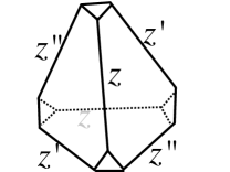
Figure 2: An ideal tetrahedron $\Delta$, tetrahedron with truncated vertices. Hyperbolic structures of $\Delta$ are parameterized by edge parameters $(z:=e^{Z},z^{\prime}:=e^{Z^{\prime}},z^{\prime\prime}=e^{Z^{\prime\prime}})$ satisfying relations $z^{\prime}=\frac{1}{1-z}$ and $z^{\prime\prime}=1-z^{-1}$. These parameters assigned to each pair of boundary edges, as shown in the figure. Geometrically, the logarithm parameters ($Z,Z^{\prime},Z^{\prime\prime}$) measure complex dihedral angles between two faces meeting at the edges. Imaginary parts of these logarithm parameters take values between 0 and $\pi$.

Here $K$ is a link on $S^{3}$ of $|K|$ components. A link complement $S^{3}\backslash K$ is a 3-manifold obtained by removing the tubular neighborhood (topologically $|K|$ copies of solid-tori) of a link $K$ from a 3-sphere $S^{3}$. The manifold has $|K|$ torus boundaries and 1-cycles around the link are called ‘meridians’ and 1-cycles along the link are ‘longitudes’. The 3-manifold $M$ in (30) is obtained by gluing $S$ solid-tori back to the link complement with following identification :

$$p_{\alpha}(\textrm{$\alpha$-th meridian})+q_{\alpha}(\textrm{$\alpha$-th longitude})$$

$$\sim(\textrm{contractable cycle in $\alpha$-th solid-torus})\;.$$ (32)

The procedure of gluing solid-torus is called $(p_{\alpha},q_{\alpha})$-Dehn filling. $(p_{\alpha},q_{\alpha})$ is a pair of coprime numbers and the ratio $p_{\alpha}/q_{\alpha}$ is called ‘slopes’. In short, the 3-manifold is obtained by gluing $T$ ideal tetrahedrons and $S$ solid-tori:

$$T\;:\;\sharp\textrm{ of ideal tetrahedrons}\;,\quad S\;:\;\sharp\textrm{ of solid-tori}\;.$$ (33)

The resulting 3-manifold $M$ has $(|K|-S)$ torus boundaries and when $S=|K|$ it is a closed 3-manifold. Any closed 3-manifold $M$ can be obtained by a Dehn surgery on $S^{3}$ 10.2307/1970373 ; Wallace1960 .

State-integral model

State-integrals give a finite-integral representation of the CS ptn by properly ‘quantizing’ the ideal triangulation (31) and the Dehn filling (32). There are several state-integral models 2007JGP….57.1895H ; Dimofte:2011gm ; Andersen:2011bt , which are believed to be equivalent, based on an ideal triangulation of $M$. We use the one developed by Dimofte and incorporate Dehn filling into the state-integral model to cover more general class of 3-manifolds such as closed hyperbolic 3-manifolds. One systematic way of specifying the gluing rule of an ideal triangulation is using (generalized) Neunmann-Zagier (NZ) datum $(A,B,C,D;f,f^{\prime\prime},\nu,\nu_{p})$, refer to Dimofte:2012qj for the definition, where $A,B,C,D$ are $T\times T$ matrices forming $Sp(2T,\mathbb{Q})$

$$\left(\begin{array}[]{cc}A&B\\ C&D\end{array}\right)\in Sp(2T,\mathbb{Q})\;,\quad\textrm{with }{\rm det}B\neq 0\;,$$ (36)

and $(f,f^{\prime\prime},\nu,\nu_{p})$ are vectors of length $T$. From these datum, the state-integral (SI) for the link complement is given by Dimofte:2012qj

$${\cal Z}_{\rm SI}(S^{3}\backslash K;X_{1},\ldots,X_{|K|};\hbar)$$

$$=\frac{1}{\sqrt{{\rm det}B}}\int\prod_{i=1}^{T}\frac{\Psi_{b}(Z_{i})dZ_{i}}{\sqrt{2\pi\hbar}}\exp\bigg{[}\frac{1}{2\hbar}\vec{Z}\cdot B^{-1}A\vec{Z}+\frac{1}{\hbar}\bigg{(}2u\cdot DB^{-1}u+(2\pi i+\hbar)f\cdot B^{-1}u$$

$$\qquad\qquad\qquad\qquad+\frac{1}{2}(i\pi+\hbar/2)^{2}f\cdot B^{-1}\nu-\vec{Z}\cdot B^{-1}\big{(}(i\pi+\hbar/2)\nu+2u\big{)}\bigg{)}\bigg{]}\;.$$ (37)

Here we define

$$u=\big{(}X_{1},\ldots,X_{|K|},0,\ldots,0\big{)}\;.$$ (38)

The quantum dilogarithm function (QDL) $\Psi_{b}$ is a wave-function on each tetrahedron. See Appendix B for the definition and basic properties of the special function. Quantizing the Dehn fillings in (32), we finally have

$${\cal Z}_{\rm SI}\big{(}M;X_{1},\ldots,X_{|K|-S};\hbar\big{)}$$

$$=\int\prod_{\alpha=1}^{S}\frac{\Delta_{b}(X_{\alpha+|K|-s};s_{\alpha},q_{\alpha})dX_{\alpha+|K|-S}}{(2\pi q_{\alpha}\hbar)^{1/2}}\exp\bigg{(}\frac{1}{\hbar}\sum_{\alpha=1}^{S}\frac{p_{\alpha}X_{\alpha+|K|-s}^{2}}{q_{\alpha}}\bigg{)}{\cal Z}_{\rm SI}\big{(}S^{3}\backslash K;X_{1},\ldots,X_{|K|};\hbar\big{)}\;,$$

$$\textrm{with }\Delta_{b}(X;s,q):=e^{-\frac{i\pi s}{2q}(b^{2}+b^{-2})}\bigg{(}e^{\frac{X}{b^{2}q}}\sinh(\frac{X-i\pi s}{q})-e^{-\frac{X}{b^{2}q}}\sinh(\frac{X+i\pi s}{q})\bigg{)}\;.$$ (39)

Here $s_{\alpha}$ is defined to be an integer satisfying $s_{\alpha}p_{\alpha}\in q_{\alpha}\mathbb{Z}-1$. See Appendix C for the derivation. The CS wave-function has following naive path-integral interpretation,

$${\cal Z}_{\rm SI}\big{(}M;X_{1},\ldots,X_{|K|-S};\hbar=2\pi ib^{2}\big{)}$$

$$=\int\frac{[d\mathcal{A}]_{X}}{(\textrm{gauge})}\exp\bigg{(}\frac{i(k+\sigma)}{8\pi}\textrm{CS}[{\cal A}]+\frac{i(k-\sigma)}{8\pi}\textrm{CS}[\bar{{\cal A}}]\bigg{)}\bigg{|}_{\eqref{3d-3d correspondence-2}}\;,\;\textrm{ where}$$

$$[d{\cal A}]_{X}\;:\;\textrm{Path-integral over $SL(2)$ gauge field on $M$ subject to}$$

$$\qquad\qquad\textrm{boundary conditions fixing }\textrm{P}e^{\oint_{I-\textrm{th merdian}}{\cal A}}=\left(\begin{array}[]{cc}e^{X_{I}}&1\\ 0&e^{-X_{I}}\end{array}\right)\;.$$ (42)

The $SL(2)$ CS wave-function is defined up to a factor Dimofte:2012qj .

$$\exp\big{(}\frac{\pi^{2}}{6\hbar}\alpha+\frac{i\pi}{4}\beta+\frac{\hbar}{24}\gamma\big{)}\;,\quad\alpha,\beta,\gamma\in\mathbb{Z}\;.$$ (43)

The factor is a purely phase factor for real $b$ and irrelevant in free-energy ${\cal F}_{b}$ computation. In the SCFT side of 3d/3d correspondence, (some parts of) the ambiguities comes from local counter-terms in a supergravity on the curved ($S^{3}_{b}$) background Closset:2012vg .

3.1.2 Perturbative invariants

Using the state-integral model above, we define the perturbative invariants which play an essential role in the 3d/3d relation (23). The state-integral model in (37) and (39) is of the form :

$${\cal Z}_{\rm SI}\big{(}M;X_{1},\ldots,X_{|K|-S};\hbar\big{)}$$

$$=\int\frac{dX_{|K|-S+1}\ldots dX_{|K|}dZ_{1}\ldots dZ_{T}}{(2\pi\hbar)^{(T+S)/2}}\;\exp\bigg{(}{\cal W}\big{(}Z_{1},\ldots,Z_{T},X_{1},\ldots,X_{|K|};\hbar\big{)}\bigg{)}\;.$$ (44)

In the limit when $\hbar\rightarrow 0$, using eq. (118)

$${\cal W}(\vec{Z},\vec{X};\hbar)\sim\frac{1}{\hbar}{\cal W}_{0}(\vec{Z},\vec{X})+{\cal W}_{1}(\vec{Z},\vec{X})+\hbar{\cal W}_{2}(\vec{Z},\vec{W})+\ldots\;.$$ (45)

Saddle point equations are

$$\bullet\;\frac{\partial{\cal W}_{0}}{\partial Z_{i}}=0\;,\quad\textrm{for }i=1,\ldots,T$$

$$\;\;\;\;\Rightarrow A\cdot\vec{Z}+B\cdot\vec{Z}^{\prime\prime}-i\pi\nu=2u\;\;\textrm{where }Z^{\prime\prime}_{i}:=\log(1-e^{-Z_{i}})\;,$$

$$\bullet\;\frac{\partial{\cal W}_{0}}{\partial X_{\alpha+|K|-S}}=0\;,\;\;\textrm{for }\alpha=1,\ldots,S$$

$$\;\;\;\;\Rightarrow p_{\alpha}X_{\alpha+|K|-S}+q_{\alpha}P_{\alpha+|K|-S}=-\textrm{sign}\big{(}\textrm{Re}[\frac{X_{\alpha+|K|-S}}{q_{\alpha}}]\big{)}\pi i\;.$$ (46)

Here $u$ is defined in (38) and we define

$$P_{\alpha+|K|-S}:=\big{(}C\cdot\vec{Z}+D\cdot\vec{Z}^{\prime\prime}-i\pi\nu_{p}\big{)}_{\alpha+|K|-S}\;.$$ (47)

Interpreting the variables $Z$ and $Z^{\prime\prime}$ as logarithmic edge parameters of ideal tetrahedrons, these are nothing but gluing equations for the 3-manifold studied in NZ:1985 . Solutions to the gluing solution give $SL(2)$ flat connections on $M$. Refer to Dimofte:2013iv for explicit construction of holonomy representation of a flat connection from a solution to the gluing equations. In the map, the solution corresponding to the flat connection ${\cal A}^{\overline{\rm hyp}}$ is characterized by following conditions:

$$0<\textrm{Im}[Z_{i}]<\pi\;,\quad\textrm{for all $i=1,\ldots,T$\;}\;\;\quad\quad(\textrm{hyperbolic})$$

$$X_{1}=\ldots=X_{|K|-S}=0\;\qquad\qquad\qquad\qquad\;\;\;(\textrm{complete})$$ (48)

Under the first condition, logarithmic edge parameter $Z_{i}$ determines a hyperbolic structure on $\Delta_{i}$, see Fig 2. The gluing equations are conditions for the hyperbolic structures to be glued smoothly and give a hyperbolic structure on the 3-manifold. For complete hyperbolic structure, we additionally need the second conditions requring the meridian holonomies in eq. (42) are parabolic. Near each $\mathbb{T}^{2}$-boundary, the complete hyperbolic metric on $M$ are locally

$$ds^{2}=\frac{1}{z^{2}}\big{(}dz^{2}+ds^{2}_{\mathbb{T}^{2}}\big{)}\;.$$ (49)

Here $z$ is the (inward) direction transverse to the boundary $\mathbb{T}^{2}$. Using the metric, one can check that the flat connection ${\cal A}^{\overline{\textrm{hyp}}}$ in (18) have parabolic meridian holonomies. For the case when $M$ is hyperbolic and we use an idea triangulation with positive angle structure, there is an unique solution for eq. (46) and (48) modulo the Weyl-symmetries $(\mathbb{Z}_{2})^{S}$.

$$(\mathbb{Z}_{2})^{S}\;:\;X_{\alpha+|K|-S}\rightarrow\pm X_{\alpha+|K|-S}\;\;\;\textrm{for }\alpha=1,\ldots,S\;.$$ (50)

The unique saddle point corresponds to the flat connection ${\cal A}^{\overline{\textrm{hyp}}}$ and we denote

$$\big{(}X_{\alpha+|K|-S}^{\overline{\textrm{hyp}}},Z_{i}^{\overline{\textrm{hyp}}}\big{)}:=\textrm{A solution satisfying eq.~{}\eqref{saddle point equations} and \eqref{geometric gluing solution}}\;.$$ (51)

For non-hyperbolic $M$, there’s no saddle point satisfying these conditions. The formal perturbative expansion of the state-integral around the saddle point defines the perturbative ptn ${\cal Z}_{\rm pert}^{\overline{\textrm{hyp}}}(M;\hbar)$ (15):

$${\cal Z}^{\overline{\textrm{hyp}}}_{\rm pert}\big{(}M;\hbar\big{)}:=2^{S}\times{\cal Z}_{\rm pert;SI}^{\overline{\textrm{hyp}}}\big{(}M;\vec{X}=\vec{0};\hbar\big{)}\;,$$

$$:=2^{S}\times\big{[}\textrm{Perturbative expansion of ${\cal Z}_{\rm SI}\big{(}M;\vec{X}=\vec{0};\hbar\big{)}$ around \eqref{the saddle point in state-integral}}\big{]}\;.$$ (52)

The overall factor $2^{S}$ comes from the fact that there are that many saddle points related by Weyl-symmetries and they all give same perturbative expansion. The state-integral is finite dimensional integration and thus the formal expansion coefficients $\{S^{\overline{\textrm{hyp}}}_{n}(M)\}_{n=0}^{\infty}$ are well-defined without any issue of regularization. Refer to Dimofte:2012qj for perturbative expansion of the state-integral model in (37) using Feynman diagram.

Examples $(S^{3}\backslash{\bf 5^{2}_{1}})_{(p,q)}$

White-head link (${\bf 5^{2}_{1}}$) is one of simplest hyperbolic link with two components.

Figure 3: White-head link (${\bf{\color[rgb]{1,0,0}5}^{2}_{\color[rgb]{0,0,1}1}}$), the 1st one among links with 2 components and 5 crossings.

The link complement can be decomposed into 4 ideal tetrahedrons (see Appendix A) :

$$S^{3}\backslash{\bf 5^{2}_{1}}=\bigg{(}\bigcup_{i=1}^{4}\Delta_{i}\bigg{)}/\sim\;.$$ (53)

Using the ideal triangulation, the corresponding state-integral is given by

$${\cal Z}_{\rm SI}\big{(}S^{3}\backslash{\bf 5^{2}_{1}};X_{1},X_{2};\hbar\big{)}=\frac{1}{\sqrt{2}}\int\prod_{i=1}^{4}\frac{\Psi_{b}(Z_{i})dZ_{i}}{\sqrt{2\pi\hbar}}\exp\bigg{[}\frac{2X_{1}(2Z_{1}+2Z_{4}-\hbar-2i\pi)-2Z_{3}Z_{4}}{2\hbar}$$

$$\;\;\;\;\quad+\frac{2X_{2}(-2Z_{2}-2Z_{4}+\hbar+2i\pi)+(Z_{1}+Z_{2}-Z_{3})(Z_{1}+Z_{2}-Z_{3}-\hbar-2i\pi)}{2\hbar}\bigg{]}\;.$$ (54)

Applying the quantum Dehn filling formula (39) to the above integral, we obtain the state-integral for $M=(S^{3}\backslash{\bf 5^{2}_{1}})_{(p,q)}$. For example, when $(p,q)=(5,-1)$

$${\cal Z}_{\rm SI}\big{(}(S^{3}\backslash{\bf 5^{2}_{1}})_{(5,-1)};X_{1};\hbar\big{)}$$

$$=\int\frac{2\sinh(X_{2})\sinh(X_{2}/b^{2})dX_{2}}{\sqrt{2\pi\hbar}}\exp\big{(}-\frac{5X_{2}^{2}}{\hbar}\big{)}{\cal Z}_{\rm SI}(S^{3}\backslash{\bf 5^{2}_{1}};X_{1},X_{2};\hbar)\;.$$ (55)

In the case, the resulting 3-manifold is turned out to be a 3-manifold called ‘sister of figure-eight knot-complement’. In SnapPy’s notation snappy , the 3-manifold is denoted as $m003$ and allows an ideal triangulation using two tetrahedrons (see Appendix A):

$$m003=(S^{3}\backslash{\bf 5^{2}_{1}})_{(5,-1)}=\bigg{(}\bigcup_{i=1}^{2}\Delta_{i}\bigg{)}/\sim\;.$$ (56)

From the ideal triangulation, we have an alternative expression for the state-integral model

$${\cal Z}_{\rm SI}(m003;X_{1};\hbar) =\int\prod_{i=1}^{2}\frac{\Psi_{b}(Z_{i})dZ_{i}}{\sqrt{2\pi\hbar}}\exp\bigg{[}\frac{X_{1}(8Z_{1}+4Z_{2}-2\hbar-4i\pi)+8X_{1}^{2}}{2\hbar}$$

$$\qquad\qquad+\frac{2Z_{1}(Z_{2}-\hbar-2i\pi)+Z_{2}(Z_{2}-\hbar-2i\pi)+4Z_{1}^{2}}{2\hbar}\bigg{]}\;.$$ (57)

One can check that both expressions, eq. (55) and eq. (57), give same perturbative invariants $S^{\overline{\textrm{hyp}}}_{n}(M)$ modulo (43) :

$$S^{\overline{\textrm{hyp}}}_{0}(m003)=S^{\overline{\textrm{hyp}}}_{0}\big{(}(S^{3}\backslash{\bf 5^{2}_{1}})_{(5,-1)}\big{)}=(1.64493\,-2.02988i)\;,$$

$$S^{\overline{\textrm{hyp}}}_{1}(m003)=S^{\overline{\textrm{hyp}}}_{1}\big{(}(S^{3}\backslash{\bf 5^{2}_{1}})_{(5,-1)}\big{)}=(-0.621227+1.309i)\;,$$

$$S^{\overline{\textrm{hyp}}}_{2}(m003)=S^{\overline{\textrm{hyp}}}_{2}\big{(}(S^{3}\backslash{\bf 5^{2}_{1}})_{(5,-1)}\big{)}=(0.0104167\,+0.0701641i)\;.$$

We did similar consistency checks for other examples, $(S^{3}\backslash{\bf 5^{2}_{1}})_{(3,-2)}=m007,(S^{3}\backslash{\bf 5^{2}_{1}})_{(5,-2)}=m006$ and $(S^{3}\backslash{\bf 5^{2}_{1}})_{(2,-3)}=m053$. The matches are delicate and strongly suggests that the state-integral model gives at least the correct perturbative invariants. We leave the general proof showing topological invariance of the perturbative series as future work.

3.1.3 Examples : $M=(S^{3}\backslash{\bf 5^{2}_{1}})_{(5,-1),(p,q)}$

Here we give concrete examples of central charge computation for closed hyperbolic 3-manifolds $M$. The most technically non-trivial step in (3) is extracting the perturbative invariants $\{S_{n}^{\overline{\textrm{hyp}}}\}_{n=0}^{\infty}$ from the state-integral model and performing their Borel resummation. Since the central charge is related to the squashed 3-sphere ptn around $b=1$, which corresponds to $\hbar=2\pi i=o(1)$, we need to take into account of sufficiently higher loop corrections to give a valid approximation. To circumvent the difficulty, we use a following alternative definition of ${\cal Z}^{\overline{\textrm{hyp}}}$:

$${\cal Z}^{\overline{\textrm{hyp}}}(M;\hbar)$$

$$:=\big{(}\textrm{Integration of the ${\cal Z}_{\rm SI}(M;\vec{X}=\vec{0};\hbar)$ in \eqref{form of state-integral model} along a Contour $\Gamma^{\overline{\textrm{hyp}}}(b)$}\big{)}\;,$$ (58)

where the converging continuous Contour $\Gamma^{\overline{\textrm{hyp}}}(b)$

$$\Gamma^{\overline{\textrm{hyp}}}(b):=\big{\{}Z_{i}=m_{i}+i\mathbb{Z}_{i}(b;\vec{m}),\;X_{|K|-S+\alpha}=m_{T+\alpha}+i\mathbb{X}_{\alpha}(b;\vec{m})\;:\;\vec{m}\in\mathbb{R}^{T+S}\big{\}}_{i=1,\ldots,T}^{\alpha=1,\ldots,S}$$

$$\qquad\qquad\;\;\subset\mathbb{C}^{T+S}\;,$$

is chosen to satisfy following conditions

$$0<\mathbb{Z}_{i}(b;\vec{m})<\pi(1+b^{2})\;,\quad\textrm{ $\forall\vec{m}\in\mathbb{R}^{T+S}$ and $\forall i=1,\ldots,T$\;.}$$ (59)

From Picard-Lefschetz and resurgence theory (see, for example, Dunne:2015eaa and reference therein) and the uniqueness of saddle point (51), we expect that for hyperbolic $M$

$$a)\textrm{ There is an unique converging non-trivial contour satisfying the conditions in \eqref{geometric contour} ,}$$

$$b)\textrm{ Two definitions of ${\cal Z}^{\overline{\textrm{hyp}}}$ in \eqref{Z^{conj} from borel sum} and \eqref{Z^{conj} from state-integral} are equivalent. }$$ (60)

For non-hyperbolic $M$, on the other hand, we expect that there is no converging contour satisfying (59). It would be interesting to check $a)$ and $b)$ explicitly using examples other than the figure-eight knot case in (24) and (25).

In the below, we give the explicit form of unique converging cycle for several cases and numerically evaluate the central charges using the ‘short-cut’ (58). For better reliability, it is recommended to do central charge computation again using the Borel resummation of the perturbative invariants which calls for an efficient algorithm of computing the invariants, such as Feynman diagrams Dimofte:2012qj .

Weeks manifold $=(S^{3}\backslash{\bf 5^{2}_{1}})_{(5,-1)(5,-2)}=({m003})_{(5,-2)}$

Weeks manifold is the smallest volume hyperbolic 3-manifold. The state-integral is given by (sloppy in the overall factor of the form (43))

$${\cal Z}^{\overline{\textrm{hyp}}}\big{(}{\it Weeks};\hbar=2\pi ib^{2}\big{)}$$

$$=\int_{\Gamma^{\overline{\textrm{hyp}}}_{{\it Weeks}}}\frac{dZ_{1}dZ_{2}dX}{(2\pi)^{3}\sqrt{2}}\big{(}2\cosh(\frac{bX}{2})\cosh(\frac{X}{2b})\big{)}\psi_{b}(Z_{1})\psi_{b}(Z_{2})$$

$$\quad\quad\times e^{-\frac{1}{2}(b+b^{-1})(2Z_{1}+Z_{2}+2X)-\frac{i}{4\pi}(4Z_{1}^{2}+Z_{2}^{2}+4Z_{2}X+3X^{2}+2Z_{1}Z_{2}+8Z_{1}X)}\;,$$

$$\simeq\int_{{\gamma}^{\overline{\textrm{hyp}}}_{{\it Weeks}}}\frac{dZ_{1}dX}{(2\pi)^{2}\sqrt{2}}\big{(}2\cosh(\frac{bX}{2})\cosh(\frac{X}{2b})\big{)}\psi_{b}(Z_{1})\psi_{b}(2X+Z_{1})$$

$$\qquad\times\exp\big{[}-(b+b^{-1})(Z_{1}+X)-\frac{i}{4\pi}(4Z_{1}^{2}+3X^{2}+8Z_{1}X)\big{]}\;.$$

Using an identity of QDL (123), we first integrated out $Z_{2}$ along a cycle $\mathbb{E}_{2X+Z_{1}}$. The contour $\Gamma^{\overline{\textrm{hyp}}}_{\it Weeks}$ is a bundle over a 2d cycle $\gamma^{\overline{\textrm{hyp}}}_{\rm Weeks}\subset\mathbb{C}^{2}_{X,Z_{1}}$ whose fiber is the $\mathbb{E}_{2X+Z_{1}}$:

$$\mathbb{E}_{2X+Z_{1}}\;\longrightarrow\;\; \Gamma^{\overline{\textrm{hyp}}}_{Weeks}$$

$$\downarrow$$ (61)

$$\gamma^{\overline{\textrm{hyp}}}_{\it Weeks}$$

One particular choice of converging contour $\gamma^{\overline{\textrm{hyp}}}_{\it Weeks}$ in the reduced two-dimensional integration is

$$\gamma^{\overline{\textrm{hyp}}}_{\it Weeks}:=\big{\{}\big{(}Z_{1},X\big{)}=\big{(}m_{1}+iA_{\it Weeks}(m_{1},m_{2}),m_{2}+iB_{\it Weeks}(m_{1},m_{2})\big{)}\;:\;(m_{1},m_{2})\in\mathbb{R}^{2}\big{\}}\subset\mathbb{C}^{2}\;,$$

where the continuous functions $A_{\it Weeks}(m_{1},m_{2})$ and $B_{\it Weeks}(m_{1},m_{2})$ have following asymptotic behavior :

$$\big{\{}A_{\it Weeks},B_{\it Weeks}\big{\}}=\begin{cases}\big{\{}\frac{(b+b^{-1})}{8},0\big{\}}&\mbox{if }m_{1}\geq\Lambda\;\;\;\;\;\textrm{ and }\;\;\;m_{2}\geq\Lambda\\ \big{\{}\frac{27(b+b^{-1})}{20},-\frac{11(b+b^{-1})}{20}\big{\}}&\mbox{if }m_{1}\geq\Lambda\;\;\;\;\;\textrm{ and }\;\;\;m_{2}<-\Lambda\\ \big{\{}\frac{(b+b^{-1})}{8},{\rm min}(\frac{|m_{1}|}{2|m_{2}|},1)(b+b^{-1})\big{\}}&\mbox{if }m_{1}\leq-\Lambda\;\;\textrm{ and }\;\;\;m_{2}\geq\Lambda\\ \big{\{}2(b+b^{-1}),-\frac{1}{2}(b+b^{-1})\big{\}}&\mbox{if }m_{1}\leq-\Lambda\;\;\textrm{ and }\;\;\;m_{2}\leq-\Lambda\\ \end{cases},$$

with a proper positive number $\Lambda$, say $5$. For other asymptotic regions, the functions $(A_{Weeks},B_{Weeks})$ are given by a linear interpolation of the above. For example,

$$A_{\it Weeks}(m_{1},m_{2})=\frac{1}{2\Lambda}(m_{1}+\Lambda)A_{\it Weeks}(\Lambda,m_{2})+\frac{1}{2\Lambda}(\Lambda-m_{1})A_{\it Weeks}(-\Lambda,m_{2})\;,$$

$$\textrm{when }-\Lambda\leq m_{1}\leq\Lambda\textrm{ and }m_{2}\geq\Lambda\;.$$ (62)

The function can be continuously extended to the remaining finite region $[-\Lambda,\Lambda]^{2}\subset\mathbb{R}^{2}$ without touching poles, see (122), in the integrand. Since the integrand is locally holomorphic, small deformations of the contour do not change the final integration. The final result only depends on an homology class of the contour and the extension to the finite region is unique as an element of the homology. Using the contour, we numerically compute

$$c_{T}(T[{\it Weeks}]) =-\frac{8}{\pi^{2}}\textrm{Re}\bigg{[}\frac{\partial_{b}^{2}{\cal Z}^{\overline{\textrm{hyp}}}\big{(}{\it Weeks};\hbar=2\pi ib^{2}\big{)}}{{\cal Z}^{\overline{\textrm{hyp}}}\big{(}{\it Weeks};\hbar=2\pi ib^{2}\big{)}}\bigg{]}_{b=1}\;,$$

$$\simeq 0.93\;.$$ (63)

Thurston manifold $=(S^{3}\backslash{\bf 5^{2}_{1}})_{(5,-1),(1,-2)}=(m003)_{(1,-2)}$

It is the second smallest hyperbolic closed 3-manifold. After integrating $Z_{2}$ using the identity (123), the state-integral model reduced to

$${\cal Z}^{\overline{\textrm{hyp}}}\big{(}{\it Thurston};\hbar=2\pi ib^{2}\big{)}$$

$$=\int_{{\gamma}^{\overline{\textrm{hyp}}}_{\it Thurston}}\frac{dZ_{1}dX}{(2\pi)^{2}\sqrt{2}}\big{(}2\cosh(\frac{bX}{2})\cosh(\frac{X}{2b})\big{)}\psi_{b}(Z_{1})\psi_{b}(2X+Z_{1})$$

$$\qquad\times\exp\big{[}-(b+b^{-1})(Z_{1}+X)-\frac{i}{4\pi}(4Z_{1}^{2}+7X^{2}+8Z_{1}X)\big{]}\;.$$ (64)

The converging contour can be constructed in the same way as for $M={\it Weeks}$ case using

$$\big{\{}A_{\it Thurston},B_{\it Thurston}\big{\}}=\begin{cases}\big{\{}\frac{(b+b^{-1})}{8},0\big{\}}&\mbox{if }m_{1}>\Lambda\;\;\;\;\;\textrm{ and }\;\;\;m_{2}>\Lambda\\ \big{\{}\frac{(b+b^{-1})}{2},\frac{3(b+b^{-1})}{4}\big{\}}&\mbox{if }m_{1}>\Lambda\;\;\;\;\;\textrm{ and }\;\;\;m_{2}<-\Lambda\\ \big{\{}2(b+b^{-1}),-\frac{7}{8}(b+b^{-1})\big{\}}&\mbox{if }m_{1}<-\Lambda\;\;\textrm{ and }\;\;\;m_{2}>\Lambda\\ \big{\{}\frac{(b+b^{-1})}{4},(b+b^{-1})\big{\}}&\mbox{if }m_{1}<-\Lambda\;\;\textrm{ and }\;\;\;m_{2}<-\Lambda\\ \end{cases}.$$

Using the contour, we numerically obtain

$$c_{T}(T[{\it Thurston}])\simeq 1.01\;.$$ (65)

(5,-1)-Dehn filling on $m003$, $(S^{3}\backslash{\bf 5^{2}_{1}})_{(5,-1),(5,-1)}=(m003)_{(5,-1)}$

The reduced state-integral model for this case is

$${\cal Z}^{\overline{\textrm{hyp}}}\big{(}m003_{-5};\hbar=2\pi ib^{2}\big{)}$$

$$=\int_{{\gamma}^{\overline{\textrm{hyp}}}_{m003_{-5}}}\frac{dZ_{1}dX}{(2\pi)^{2}}\big{(}2\sin(bX)\sin(bX/2)\big{)}\psi_{b}(Z_{1})\psi_{b}(2X+Z_{1})$$

$$\qquad\times\exp\big{[}-(b+b^{-1})(Z_{1}+X)-\frac{i}{4\pi}\big{(}4Z_{1}^{2}-2X^{2}+8Z_{1}X\big{)}\big{]}\;.$$

For the contour, we use

$$\big{\{}A_{m003_{-5}},B_{m003_{-5}}\big{\}}=\begin{cases}\big{\{}\frac{(b+b^{-1})}{8},0\big{\}}&\mbox{if }m_{1}>\Lambda\;\;\;\;\;\textrm{ and }\;\;\;m_{2}>\Lambda\\ \big{\{}2(b+b^{-1}),-\frac{9(b+b^{-1})}{10}\big{\}}&\mbox{if }m_{1}>\Lambda\;\;\;\;\;\textrm{ and }\;\;\;m_{2}<-\Lambda\\ \big{\{}\frac{(b+b^{-1})}{8},(b+b^{-1})\big{\}}&\mbox{if }m_{1}<-\Lambda\;\;\textrm{ and }\;\;\;m_{2}>\Lambda\\ \big{\{}2(b+b^{-1}),-\frac{(b+b^{-1})}{2}\big{\}}&\mbox{if }m_{1}<-\Lambda\;\;\textrm{ and }\;\;\;m_{2}<-\Lambda\\ \end{cases}.$$

Using the contour, numerically we find

$$c_{T}(T[(m003)_{(5,-1)}])\simeq 1.28\;.$$ (66)

Integral Dehn fillings on $m003$, $(S^{3}\backslash{\bf 5^{2}_{1}})_{(5,-1),(p,1)}=(m003)_{(p,1)}$ with $p\geq 5$

The reduced state-integral model is

$${\cal Z}^{\overline{\textrm{hyp}}}\big{(}m003_{p};\hbar=2\pi ib^{2}\big{)}$$

$$=\int_{{\gamma}^{\overline{\textrm{hyp}}}_{m003_{p}}}\frac{dZ_{1}dX}{(2\pi)^{2}}\big{(}2\sinh(bX)\sin(X/b)\big{)}\psi_{b}(Z_{1})\psi_{b}(2X+Z_{1})$$

$$\qquad\times\exp\big{[}-(b+b^{-1})(Z_{1}+X)-\frac{i}{4\pi}\big{(}4Z_{1}^{2}+(8+2p)X^{2}+8Z_{1}X\big{)}\big{]}\;.$$

One particular choice of $\gamma^{\overline{\textrm{hyp}}}_{m003_{p}}$ ($p\geq 5$) is

$$\gamma^{\overline{\textrm{hyp}}}_{m003_{p}}:=\bigg{\{}\big{\{}Z_{1},X\big{\}}=\big{\{}m_{1}+(b+b^{-1})i,m_{2}-\frac{2(b+b^{-1})i}{3\pi}\arctan(m_{2})\big{\}}\;:\;m_{1},m_{2}\in\mathbb{R}\bigg{\}}\subset\mathbb{C}^{2}\;.$$

3.2 Comments on BPS operator spectrum

Here we present some difficulties in determining chiral operator spectrum of wrapped M5-brane theory $T[M]$. The difficulties are closely related to the two challenges in 3d/3d story posed in Chung:2014qpa : a) recovering full flat connections on $M$ some of which are missing in ideal triangulations b) categorification/refinement of complex Chern-Simons theory.

Superconformal index computation

Superconformal index (SCI) is a physical quantity which contains information about BPS operator spectrum. Via the 3d/3d relation, it is also related to a complex CS ptn Dimofte:2011py ; Gang:2013sqa ; Yagi:2013fda ; Lee:2013ida as $S^{3}_{b}$-ptn. But there is a crucial difference between two CS theories corresponding to SCI and $S^{3}_{b}$-ptn: whether the non-quantized CS level $\sigma$ is real or purely imaginary,

$$\sigma\in i\mathbb{R}\;\quad\textrm{for superconformal index}\;,$$

$$\sigma\in\mathbb{R}\;\quad\;\;\textrm{for $S^{3}_{b}$-ptn with real $b$}\;.$$

For purely imaginary $\sigma$, unitarity structure of the complex CS theory is usual and $\bar{{\cal A}}$ con be considered as the complex conjugation of ${\cal A}$. In the case, all flat connections contribute to the CS ptn since they are on the contour, $\bar{{\cal A}}={\cal A}^{*}$ Witten:2010cx (see also the sec 2.1 of Gang:2015wya ). However, the construction based on ideal triangulation misses some branches of flat-connections including Abelian branch Chung:2014qpa . Thus, the state-integral based on ideal triangulation can not give correct full SCI of $T[M]$. For real $\sigma$, on the other hand, the situation is more subtle and it is difficult to say which flat connections may contribute to the CS ptn from view-point of purely complex CS theory. Our basic assumption motivated by physical principles (holography and unitarity of wrapped M5-branes SCFTs) is that the ${\cal A}^{\overline{\textrm{hyp}}}$ is the only relevant flat connection appearing in the 3d/3d relation for $S^{3}_{b}$-ptn, see eq. (21) and (23). The flat connection is always captured in an ideal triangulation and the $S^{3}_{b}$-ptn can be computed using the ‘incomplete’ state-integral as we proposed in the previous sections.

Non-trivial mixing of the IR R-charge

One may think the superonformal IR $R$-symmetry $U(1)^{\rm IR}_{R}$ of 3d SCFT $T[M]$ comes from a $SO(2)$ subgroup of the $SO(5)$ R-symmetry in the original 6d $(2,0)$ theory. If it is the case, spectrum of the $U(1)^{\rm IR}_{R}$ should be quantized and so should $\Delta_{\Phi}$ (conformal dimension of a chiral primary $\Phi$). Actually, however, the correct 3d IR $R$-charge is a linear combination of $U(1)_{R}$ and $U(1)_{t}$ of $T^{\rm full}[M]$, see Table 2.

$$\bigg{(}U(1)^{\rm IR}_{R}\textrm{ of }T[M]\bigg{)}\;\subset\;\bigg{(}U(1)_{R}\times U(1)_{t}\textrm{ of }T^{\rm full}[M]\bigg{)}\;.$$ (67)

The correct IR mixing can be determined after identifying the ‘Higgsing/deformation’ procedure in eq. (5). The complex mass parameter for the $U(1)_{t}$ plays a role as a refinement parameter in refined Chern-Simons theory Chung:2014qpa . Holographically the mixing can be studied by analyzing KK spectrum on the holographic dual background (9). There is an unique massless vector field on the $AdS_{4}$ background which is given by a linear combination of the form Donos:2010ax

$$A^{\rm IR}=A+\frac{3}{g}C\;,$$ (68)

where $g$ is a constant in the supergravity solution related to the number of M5-branes. $A$ is an one-form obtained by KK-reduction of metric along the $S^{1}$ isometry direction in the $S^{4}$ and $C$ is an one-form by KK-reduction of four-form field strength $G_{4}=dC_{3}$ along a 3-cycle inside the internal manifold $M\times S^{4}$. The holographic dual of $T^{\rm full}_{N}[M]$ should have two massless vector fields, $A$ and $C$, corresponding to $U(1)_{R}$ and $U(1)_{t}$ respectively. Since an integration of the Ramond-Ramond 4-form flux $G_{4}=dC_{3}$ measures M2-brane charge, the $U(1)_{t}$-charge counts M2-branes wrapping a 3-cycle inside $M\times S^{4}$. It is compatible with the interpretation of $U(1)_{t}$ in Gukov:2016gkn .

4 Kink CFTs in superconformal bootstrap

In this section, we analyze the SCFTs constructed in the previous section by wrapped two M5-branes on closed hyperbolic 3-manifolds in the eye of numerical superconformal bootstrap. Studies on numerical bootstrap for 3d ${\cal N}=2$ SCFT was given in Bobev:2015vsa ; Bobev:2015jxa . One of the notable features in their work was existence of three kinks for $\bar{\Phi}\Phi$ operator dimensions bounds. From the numerical bootstrap studies of Ising model and $O(N)$ vector model, there are good indications that interesting theory (known or unknown) exists with CFT spectrum at the kink location ElShowk:2012ht ; El-Showk:2014dwa ; El-Showk:2013nia ; Kos:2013tga ; Kos:2014bka ; Kos:2015mba ; Kos:2016ysd . Sudden change of numerical bounds indicate rearrangement of operator spectrum, such as certain operator decoupling, indicating interesting physical theory associated with it El-Showk:2014dwa .

The identity of the first kink is well described by critical Wess-Zumino(cWZ) model at $\Delta_{\Phi}=\frac{2}{3}$ whereas the second kink at $\Delta_{\Phi}=\frac{3}{4}$ is suggested to be coming from kinematic constraints . The third kink seems interesting as it appears to show similar features as other interesting theories identifiable in the study of conformal bootstrap. As far as we know, there are currently no good identification to any known SCFT construction for the third kink. Similar exotic kink also appears in 4d ${\cal N}=1$ SCFT Poland:2011ey ; Poland:2015mta , and attempts to construct candidate theory for the kink Xie:2016hny ; Buican:2016hnq .

First note that, we can easily exclude the possibility that the first kink SCFT (cWZ) as an wrapped M5-branes CFT $T[M]$. Comparing the $S^{3}_{b}$ free-energy at small $b$:

$$\lim_{b\rightarrow 0}2\pi b^{2}{\cal F}_{b}(\textrm{cWZ})=\textrm{Re}[i\mathrm{Li}_{2}(e^{-2i\pi/3})]\simeq 0.6766$$

$$<\textrm{vol}(weeks)=0.9427\leq\textrm{vol}(M)=\lim_{b\rightarrow 0}2\pi b^{2}{\cal F}_{b}(T[M])\textrm{ for any $M$}$$

$$\Rightarrow\lim_{b\rightarrow 0}2\pi b^{2}{\cal F}_{b}(\textrm{cWZ model})<\lim_{b\rightarrow 0}2\pi b^{2}{\cal F}_{b}(T[M])\textrm{ for any $M$}$$ (69)

In the second line, we use eq. (10) and the fact that the Weeks manifold has smallest hyperbolic volume. We note that this argument does not exclude the possibility that the minimal SCFT can be realized as a SCFT of generalized wrapped M5-branes system, such as including ‘irregular’ co-dimension two defects in 6d $(2,0)$ theory along whole 3d spacetime and a link $K$ inside a closed 3-manifold $M$.

Now we focus on possibility whether SCFTs constructed by wrapped M5-branes on hyperbolic 3-manifolds are candidates for the SCFT associated with third kink .

4.1 Third kink SCFT in superconformal boostrap

Let us first review, the salient properties of the third kink observed in Bobev:2015vsa ; Bobev:2015jxa :

• Chiral primary operator $\Phi$ with dimension $\Delta_{\Phi}\approx 0.86$.

• Central charge of the kink solution is $c_{T}\approx 0.93$.

• $\Phi$ has a chiral ring relation $\Phi^{2}\sim 0$.

Recall that normalization for $c_{T}$ is given as in (29).

In obtaining the numerical bounds authors of Bobev:2015vsa ; Bobev:2015jxa performed moderate numerics in order to observe global patterns in large parameter space with various spacetime dimensions. Here moderate numerics means in the sense of space of linear functional $\alpha$ in running numerical bootstrap (for a review see Rychkov:2016iqz ; Simmons-Duffin:2016gjk ; Poland:2016chs )

$$\alpha(F)=\sum_{m+n\leq\Lambda}a_{mn}\partial^{m}_{z}\partial^{n}_{\bar{z}}F(z,\bar{z})\Big{|}_{z=\bar{z}=\tfrac{1}{2}}$$ (70)

where $\Lambda$ is a cutoff introduced to make the problem finite. We are interested in constraints for $\Lambda\rightarrow\infty$. If numerics converges fast moderate value of $\Lambda$ can be sufficient, however there are cases(e.g. Beem:2014zpa ; Beem:2015aoa ; Poland:2015mta ; Lin:2015wcg ; Collier:2016cls ; Lin:2016gcl ) where reasonable computation do not yield converging result and requires extrapolation.

We focus on studying the numerical bounds close to the third kink and report more stringent bounds. Both upper bound on $\Delta_{\bar{\Phi}\Phi}$ and lower bound on $c_{T}$ vary as derivative order $\Lambda$ increases. The strategy is to obtain bounds at multiple high $\Lambda$ and extrapolate to infer the value of bounds if we searched for infinite space of linear functionals.

For running the numerics obtained in this section, we used the semi-definite programming formulation of the problem Poland:2011ey ; Kos:2013tga , making use of the solver SDPB Simmons-Duffin:2015qma and convenient wrapper cboot cbootOhtsky .

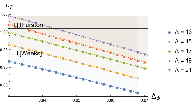
Figure 4: Lower bound of $c_{T}$ for 3d ${\cal N}=2$ SCFTs near the third kink point. The bound is obtained with most general assumption about SCFT spectrum consistent with unitarity. There is no interesting feature even at the kink point. For reference we included $c_{T}$ values computed for the $T[{\it Weeks}]$ and $T[{\it Thurston}]$ wrapped M5-brane SCFTs obtained in the previous section.

4.2 Detailed analysis of the third kink CFT data

In obtaining more stringent bound for $c_{T}$, we obtain bound directly on $c_{T}$ as opposed to extracting it from the extremal solution. The naive $c_{T}$ bound from most generic unitary spectrum do not show interesting feature and monotonically decreases as $\Delta_{\Phi}$ passes through the third kink (see Figure 4). This is most generic bound on the central charge, however it fails to capture the information of extremal theories saturating the bound. We can add extra assumption on the scalar spectrum that lightest $\Delta_{\bar{\Phi}\Phi}$ is maximal value obtained by the numerical bootstrap bound. This is similar to studying the extremal spectrum and indeed we observe the same characteristics of the third kink with extremal spectrum study was done Bobev:2015jxa for $\Lambda=13$.

We used two different ways of identifying the third kink. First is the standard way of locating where the slope of the bound changes in $\Delta_{\bar{\Phi}\Phi}$ bound or $c_{T}$ bound with maximal $\Delta_{\bar{\Phi}\Phi}$ gap imposed. Another method is to use the fact that at the kink $\Phi^{2}$ chiral primary operator decouples. Extra assumption of excluding $\Phi^{2}$ operator in the SCFT spectrum drastically change the numerical bounds near the kink. This strategy was utilized in studying similar exotic kink for 4d ${\cal N}=1$ SCFTs Poland:2015mta . This extra assumption allows us more efficient ways to study the spectrum of the kink as we can pin down the location with binary search in both $\Delta_{\Phi}$ and $\Delta_{\bar{\Phi}\Phi}$ directions. The reason that we could do binary search in $\Delta_{\Phi}$ is due to the bound having a jump at the kink (see Figure 5). Near the jump point $\Delta_{\bar{\Phi}\Phi}$ close to unitarity bound is allowed if $\Delta_{\Phi}$ is greater than the kink location and disallowed if $\Delta_{\Phi}$ is smaller than the kink location. We observe that the two approaches essentially gives the same result(e.g. Figure 5) in identifying the kink, and therefore focus on the result from the second approach imposing $\Phi^{2}$ decoupling.

First thing to observe is that the numerics does not converge as well as the first kink in the case for the third kink. For example, the location of the third kink shifts significantly as $\Lambda$ increases as see in Figure 6. Other CFT data, which relies on the location of the kink, also varies as one increases derivative order. As the numerics do not converge at reasonable order, we extrapolate to infer the CFT data for $\Lambda\rightarrow\infty$. For the $c_{T}$ with maximal $\Delta_{\bar{\Phi}\Phi}$ gap imposed (as well as other CFT data) see Figure 7 and Table 3.

$\Lambda$	$\Delta_{\Phi}$	$c_{T}$(no gap)	$c_{T}$(maximal gap)	$\Delta_{\bar{\Phi}\Phi}$
13	0.8598(2)	$0.9258$	0.9264	$2.3920(10)$
15	0.8624(2)	$0.9485$	$0.9497$	$2.3861(10)$
17	0.8647(2)	$0.9717$	$0.9731$	$2.3777(10)$
19	0.8659(2)	$0.9842$	$0.9858$	$2.3762(10)$
21	0.8669(2)	$0.9962$	$0.9976$	$2.3715(10)$
23	0.8676(2)	$1.0034$	$1.0049$	2.3700(10)
27	0.8687(2)	$1.0172$	$1.0183$	2.3663(10)
31	0.8693(2)	$1.0257$	$1.0269$	2.3643(10)
35	0.8697(2)	$1.0318$	1.0320	2.3628(10)
39	0.8700(2)	$1.0361$	1.0374	2.3624(10)
$\infty$	$0.8757/0.8713$	$1.0957/1.0723$	$1.0968/1.0709$	$2.3453/2.3554$

Table 3: Few CFT data of the third kink at various $\Lambda$ assuming no $\Phi^{2}$ in the spectrum. The bottom row indicates interpolated values for $\Lambda\rightarrow\infty$, which should be taken as suggested value rather than a strict bound. Interpolation was taken with both linear(left value) and quadratic(right value) fit respect to $\frac{1}{\Lambda}$. The values for given $\Lambda$ gives strict upper bound for $\Delta_{\bar{\Phi}\Phi}$ and strict lower bound for $\Delta_{\Phi}$ and $c_{T}$.

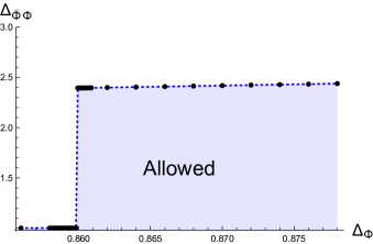
(a)

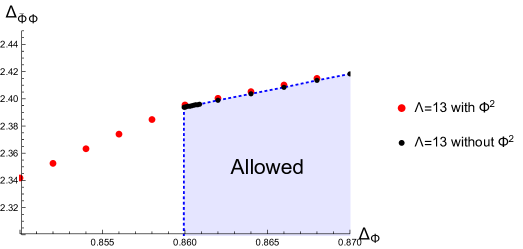
(b)

Figure 5: (a) Upper bound for dimension of $\bar{\Phi}\Phi$ with explicit assumption of $\Phi^{2}$ operator decoupling. The jump is at $(\Delta_{\Phi},\Delta_{\bar{\Phi}\Phi})=(0.8598(2),2.3937(5)).$ (b) Same bound overlapped with $\Phi^{2}$ included in the spectrum (red dots). The third kink can be identified as sudden jump (black dots) in the bound when spectrum excludes $\Phi^{2}$. The numerics was obtained with $\Lambda=13$.

According to our computation, both $T[{\it Weeks}]$ and $T[{\it Thurston}]$ are ruled out as the candidate for the third kink SCFT irrespective of interpolation(see Figure 7). Initial study from Bobev:2015jxa indicated a reasonable match with the $c_{T}$ value of $T[{\it Weeks}]$ SCFT. However, further analysis with higher order numerics excludes the potential identification. It would be interesting to check if $T[M]$ with other 3-manifolds with bigger volume can be identified as the 3rd kink.

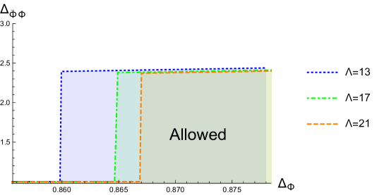
Figure 6: Assuming no $\Phi^{2}$ in the spectrum, position of the third kink shifts to larger values as $\Lambda$ increases. The numerics does not converge at reasonable order and we resort to extrapolate to infer the location at $\Lambda\rightarrow\infty$. At a given order, the kink location can be efficiently searched with binary search over $\Delta_{\Phi}$ near where the jump occurs.

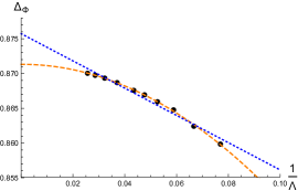
(a)

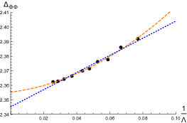
(b)

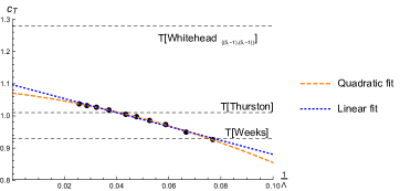
(c)

Figure 7: CFT data at the third kink as function of $\frac{1}{\Lambda}$. (a) Lower bound of location of $\Delta_{\Phi}$ (b) Upper bound on $\Delta_{\bar{\Phi}\Phi}$ (c) Lower bound on central charge with maximal $\Delta_{\bar{\Phi}\Phi}$ gap(value in (b)) imposed. The blue dashed-dotted line corresponds to the linear fit and orange dashed line corresponds to the quadratic fit of the points. Refer to Table 3 for the asymptotic value at $\tfrac{1}{\Lambda}\rightarrow 0$. For reference we included $c_{T}$ values computed for three small hyperbolic volume wrapped M5-brane SCFTs obtained in the previous section.

Appendix A Ideal triangulation of $S^{3}\backslash{\bf 5^{2}_{1}}$ and $m003$

Ideal triangulations of 3-manifolds with cusped boundaries are available in a computer software SnapPy snappy .

Whitehead link complement ($S^{3}\backslash{\bf 5^{2}_{1}}$)

The 3-manifold can be triangulated by 4 ideal tetrahedrons ($T=4$). Boundary meridian/longitude variables and indepedent internal edges $(\mathcal{C})$ are

$$X_{1}=-Z_{1}^{\prime\prime}-Z_{3}^{\prime\prime}+Z_{4}\;\;,\;\;P_{1}=\frac{Z_{1}}{2}-Z_{3}+\frac{3Z_{4}}{2}-\frac{Z^{\prime}_{1}}{2}-\frac{Z^{\prime}_{4}}{2}-Z^{\prime\prime}_{1}-Z^{\prime\prime}_{3}-\frac{Z^{\prime\prime}_{2}}{2}\;,$$

$$X_{2}=Z_{1}-Z_{2}^{\prime}-Z_{3}\;\;,\;\;P_{2}=Z_{1}-\frac{Z_{3}}{2}-\frac{Z_{4}}{2}+\frac{Z^{\prime}_{3}}{2}-\frac{Z^{\prime}_{1}}{2}-\frac{Z^{\prime}_{2}}{2}-\frac{Z^{\prime\prime}_{4}}{2}\;,$$

$$\mathcal{C}_{1}=2Z_{1}^{\prime}+Z_{1}^{\prime\prime}+2Z_{2}^{\prime}+Z_{2}^{\prime\prime}+Z_{3}+Z_{4}^{\prime\prime}-2\pi i\;,$$

$$\mathcal{C}_{2}=Z_{1}^{\prime\prime}+Z_{2}^{\prime\prime}+2Z_{3}^{\prime\prime}+Z_{3}+2Z_{4}^{\prime}+Z_{4}^{\prime\prime}-2\pi i\;.$$ (71)

Using a linear relation

$$Z_{i}+Z_{i}^{\prime}+Z_{i}^{\prime\prime}=i\pi\;,$$ (72)

the edge parameter $Z^{\prime}_{i}$ can be eliminated. After the elimination, generalized Neumann-Zagier datum $(A,B,C,D;f,f^{\prime\prime},\nu,\nu_{p})$ are determined by

$$A\cdot\left(\begin{array}[]{c}Z_{1}\\ Z_{2}\\ Z_{3}\\ Z_{4}\end{array}\right)+B\cdot\left(\begin{array}[]{c}Z^{\prime\prime}_{1}\\ Z^{\prime\prime}_{2}\\ Z^{\prime\prime}_{3}\\ Z^{\prime\prime}_{4}\end{array}\right)-i\pi\nu=\left(\begin{array}[]{c}X_{1}\\ X_{2}\\ \mathcal{C}_{1}\\ \mathcal{C}_{2}\end{array}\right)\;,\;\;C\cdot\left(\begin{array}[]{c}Z_{1}\\ Z_{2}\\ Z_{3}\\ Z_{4}\end{array}\right)+D\cdot\left(\begin{array}[]{c}Z^{\prime\prime}_{1}\\ Z^{\prime\prime}_{2}\\ Z^{\prime\prime}_{3}\\ Z^{\prime\prime}_{4}\end{array}\right)-i\pi\nu_{p}=\left(\begin{array}[]{c}P_{1}\\ P_{2}\\ \Gamma_{1}\\ \Gamma_{2}\end{array}\right)$$ (97)

$$A\cdot f+B\cdot f^{\prime\prime}=\nu\;,\quad C\cdot f+D\cdot f^{\prime\prime}=\nu_{p}\;.$$

Here $\{\Gamma_{i}\}_{i=1}^{2}$ are some linear combinations of $\vec{Z}$ and $\vec{Z}^{\prime\prime}$ chosen to satisfy

$$\left(\begin{array}[]{cc}A&B\\ C&D\end{array}\right)\in Sp(8,\mathbb{Q})\;.$$ (100)

For example, we can choose

$$\Gamma_{1}=\frac{Z_{1}}{2}-\frac{Z_{3}}{4}-\frac{Z_{4}}{4}+\frac{Z^{\prime\prime}_{1}}{4}-\frac{Z^{\prime\prime}_{2}}{2}-\frac{Z^{\prime\prime}_{3}}{4}-\frac{Z^{\prime\prime}_{4}}{4}\;,$$

$$\Gamma_{2}=\frac{Z_{1}}{2}+\frac{Z_{4}}{2}-\frac{5Z_{3}}{8}+\frac{3Z^{\prime\prime}_{1}}{8}+\frac{Z^{\prime\prime}_{4}}{8}-\frac{3Z^{\prime\prime}_{2}}{8}\;.$$ (101)

The final expression of the state-integral model is independent on the specific choice of $\Gamma_{1}$ and $\Gamma_{2}$.

Sister of figure-eight knot complement = $(S^{3}\backslash 5^{2}_{1})_{{\bf(5,-1)}}=(m003)$

The 3-manifold can be triangulated by 2 ideal tetrahedrons ($T=2$). After eliminating $(Z_{1}^{\prime},Z_{2}^{\prime})$, we have

$$X=Z_{1}^{\prime\prime}+Z_{1}-2Z_{2}-3Z_{2}^{\prime\prime}+i\pi\;,\quad P=-Z_{2}-2Z_{2}^{\prime\prime}+i\pi\;.$$

$$\mathcal{C}=Z_{1}^{\prime\prime}+2Z_{1}-Z_{2}-2Z_{2}^{\prime\prime}\;,\quad\Gamma=Z_{1}^{\prime\prime}+Z_{1}$$

Generalized Neumann-Zagier datum $(A,B,C,D;f,f^{\prime\prime},\nu,\nu_{p})$ are determined by

$$A\cdot\left(\begin{array}[]{c}Z_{1}\\ Z_{2}\end{array}\right)+B\cdot\left(\begin{array}[]{c}Z^{\prime\prime}_{1}\\ Z^{\prime\prime}_{2}\end{array}\right)-i\pi\nu=\left(\begin{array}[]{c}X\\ \mathcal{C}\end{array}\right)\;,\;\;C\cdot\left(\begin{array}[]{c}Z_{1}\\ Z_{2}\end{array}\right)+D\cdot\left(\begin{array}[]{c}Z^{\prime\prime}_{1}\\ Z^{\prime\prime}_{2}\end{array}\right)-i\pi\nu_{p}=\left(\begin{array}[]{c}P\\ \Gamma\end{array}\right)$$ (114)

$$A\cdot f+B\cdot f^{\prime\prime}=\nu\;,\quad C\cdot f+D\cdot f^{\prime\prime}=\nu_{p}\;.$$

Appendix B Quantum dilogarithm

In this appendix we collect formulas for the noncompact quantum dilogarithm (QDL) function FaddeevKashaevQuantum . The function function $\Psi_{b}(Z)$ is defined by

$$\Psi_{b}(Z):=\begin{cases}\prod_{r=1}^{\infty}\frac{1-q^{r}e^{-Z}}{1-\tilde{q}^{-r+1}e^{-\tilde{Z}}}&\mbox{if }|q|<1\\ \prod_{r=1}^{\infty}\frac{1-\tilde{q}^{r}e^{-\tilde{Z}}}{1-q^{-r+1}e^{-Z}}&\mbox{if }|q|>1\\ \end{cases}$$ (115)

with

$$q:=e^{2\pi ib^{2}}\;,\quad\tilde{q}:=e^{2\pi ib^{-2}}\;,\quad\tilde{Z}:=\frac{1}{b^{2}}Z\;.$$ (116)

Integral representation:

$$\log\Psi_{b}(Z)=\int_{\mathbb{R}+i0^{+}}\frac{e^{\frac{itZ}{\pi b}+t(b+b^{-1})}}{\sinh(bt)\sinh(b^{-1}t)}\frac{dt}{4t}\;,\quad\textrm{for $0<\textrm{Im}[Z]<2\pi(1+b^{2})$\;.}$$ (117)

Asymptotic expansion when $\hbar=2\pi ib^{2}\rightarrow 0$ :

$$\log\Psi_{b}(Z)\xrightarrow{\;\;b^{2}\rightarrow 0^{+}\;\;}\sum_{n=0}^{\infty}\frac{B_{n}\hbar^{n-1}}{n!}\textrm{Li}_{2-n}(e^{-Z})\;,\quad\textrm{for $0<\textrm{Im}[Z]<\pi$}\;.$$ (118)

Here $B_{n}$ is the $n$-th Bernoulli number with $B_{1}=1/2$. To have $b\leftrightarrow b^{-1}$ symmetry, we define

$$\log\psi_{b}(x):=\log\Psi_{b}(bx)\;.$$ (119)

At $b=1$, the QDL simplified as

$$\log\psi_{b=1}(x)=\frac{-(2\pi+ix)\log(1-e^{-x})+i\textrm{Li}_{2}(e^{-x})}{2\pi}\;.$$ (120)

As $|x|\rightarrow\infty$,

$$\log\psi_{b}(x)\quad\sim\quad \frac{-x^{2}}{4\pi i}+\frac{1}{2}(b+b^{-1})x \textrm{for Re[x]$<$0}\;,$$

$$\sim\quad 0 \textrm{for Re[x]$>$0}\;.$$ (121)

Poles of the $\psi_{b}(Z)$ are located on

$$\mathbb{Z}_{\leq 0}(2\pi ib)+\mathbb{Z}_{\leq 0}(2\pi ib^{-1})\;\;.$$ (122)

Fourier transformation:

$$\frac{e^{\frac{i\pi(b^{2}+3+b^{-2})}{12}}}{2\pi}\int_{\mathbb{E}_{y}}dx\psi_{b}(x)e^{\frac{x^{2}+2xy-2\pi ix(b+b^{-1})}{4\pi i}}=\psi_{b}(y)\quad\quad\textrm{for Im}(y)>0\;,$$

$$\mathbb{E}_{y}:=\{x+if(x)\;:\;x\in\mathbb{R}\}\subset\mathbb{}\;\textrm{where $f$ is a function satisfying}$$

$$f\rightarrow\begin{cases}-\textrm{Im}(y)+(b+b^{-1})\pi-\epsilon_{1}&\mbox{if }x\rightarrow\infty\\ \epsilon_{2}&\mbox{if }x<\Lambda\\ \end{cases}\textrm{ with small $\epsilon_{1},\epsilon_{2}>0$ and positive $\Lambda$}.$$ (123)

Appendix C Quantum Dehn filling

Classical phase space $P(\partial M)$ and its Lagrangian subvariety ${\cal L}(M)$ for the $SL(2)$ CS theory are

$$P(\partial M)=\{SL(2)\textrm{-flat connections on $\partial M=(\mathbb{T}^{2})^{|K|-S}$}\}=\big{(}P(\mathbb{T}^{2})\big{)}^{|K|-S}\;$$

$$\;\;\qquad\qquad\textrm{with }P(\mathbb{T}^{2})=(\mathbb{C}^{*})^{2}/\mathbb{Z}_{2}=\{(x,p)\in(\mathbb{C}^{*})^{2}:(x,p)\sim(1/x,1/p)\}\;,$$

$$\mathcal{L}(M)=\{SL(2)\textrm{-flat connections on $M$}\}\;.$$ (124)

Here $x$ and $p$ parametrize the $SL(2)$ gauge holonomy around each meridian and longitude respectively:

$$\textrm{P}e^{\oint_{\textrm{merdian}}{\cal A}}=\left(\begin{array}[]{cc}x&1\\ 0&1/x\end{array}\right)\;,\quad\textrm{P}e^{\oint_{\textrm{longitude}}{\cal A}}=\left(\begin{array}[]{cc}p&1\\ 0&1/p\end{array}\right)\;.$$ (129)

Quantizing them, we have

$$P(\partial M)\; \leadsto\;{\cal H}(\partial M)=\big{(}{\cal H}(\mathbb{T}^{2})\big{)}^{|K|-S}\;\;\textrm{(a Hilbert-space)}\;,$$

$${\cal L}(M)\; \leadsto\;\big{|}{\cal Z}(M)\big{\rangle}\in{\cal H}(\partial M)\qquad\;\;\;\;\textrm{(a state)}\;.$$ (130)

Quantization of the phase space $P(\mathbb{T}^{2})$ with $k=1$

Phase space ${\cal P}(\mathbb{T}^{2})$ for $SL(2)_{k,\sigma}$ CS theory with $k=1$ and $\sigma=\frac{1-b^{2}}{1+b^{2}}$ on $\mathbb{R}_{t}\times\mathbb{T}^{2}$ is give in (124) with following symplectic form ($X:=\log x,P:=\log p$):

$$\Omega=\frac{1}{\pi(1+b^{2})}dP\wedge dX+\frac{1}{\pi(1+b^{-2})}d\overline{P}\wedge d\overline{X}\;.$$ (131)

Quantization of the phase space give an infinite dimensional Hilbert-space ${\cal H}(\mathbb{T}^{2})$ whose position basis are

$$\textrm{Position bais of ${\cal H}(\mathbb{T}^{2})$}=\big{\{}|X\rangle\;:\;X\in\mathbb{C}\;,\;|X\rangle\sim=|-X\rangle\big{\}}.$$ (132)

The quantum position/momentum operators acts on the Hilbert-space as

$$\langle X|\hat{x}=\langle X|e^{X}\;,\quad\langle X|\hat{\bar{x}}=\langle X|e^{X/b^{2}}\;,\quad\langle X|\hat{p}=\langle X+i\pi b^{2}|\;,\quad\langle X|\hat{\bar{p}}=\langle X+i\pi|\;.$$ (133)

Completeness relation in ${\cal H}(\mathbb{T}^{2})$ is

$$\frac{1}{4\pi b}\int d\mu\big{|}X\big{\rangle}\big{\langle}X\big{|}=\mathbb{I}\;.$$ (134)

Quantization of Dehn filling

For a 3-manifold closed $M$ obtained by gluing two 3-manifolds $M_{1}$ and $M_{2}$ along a common $\mathbb{T}^{2}$ boundary with a $\varphi\in SL(2,\mathbb{Z})$ twist, the $SL(2)$ CS ptn is given by

$${\cal Z}_{\rm SI}(M=M_{1}\cup_{\varphi}M_{2};\hbar)=\big{\langle}{\cal Z}(M_{1})\big{|}\hat{\varphi}\big{|}{\cal Z}(M_{2})\big{\rangle}\;,$$

$$\big{|}{\cal Z}(M_{i})\big{\rangle}\in{\cal H}(\mathbb{T}^{2})\;,\quad i=1,2\;,$$

$$\hat{\varphi}\;:\;{\cal H}(\mathbb{T}^{2})\rightarrow{\cal H}(\mathbb{T}^{2})\;.$$ (135)

For solid-torus $D_{2}\times S^{1}$, the wave-function is simply given by

$$\big{\langle}X\big{|}{\cal Z}(D_{2}\times S^{1})\big{\rangle}=4\sinh(X)\sinh(X/b^{2})\;.$$ (136)

Note that solid-torus can be thought as unknot complement on $S^{3}$, $D^{2}\times S^{1}=S^{3}\backslash\mathbf{0}_{1}$, and we use the canonical polarization where the position (momentum) is an eigenvalue homonomy around the meridian (longitude). The wave-function satisfy a pair of difference equations ($q:=e^{2\pi ib^{2}},\bar{q}:=e^{2\pi ib^{-2}}$):

$$\hat{A}_{K=\mathbf{0}_{1}}(\hat{x}^{2},\hat{p},q^{1/2})\big{|}{\cal Z}(D^{2}\times S^{1})\big{\rangle}=\hat{A}_{K=\mathbf{0}_{1}}(\hat{\bar{x}}^{2},\hat{\bar{p}},\bar{q}^{1/2})\big{|}{\cal Z}(D^{2}\times S^{1})\big{\rangle}=0\;,$$

$$\textrm{where }\hat{A}_{\mathbf{0}_{1}}(\hat{x}^{2},\hat{p},q^{1/2})=\hat{p}^{2}+1-q^{1/2}\hat{p}-q^{-1/2}\hat{p}\;.$$ (137)

Regardless of whether the gauge group is $SU(2)$ or its complexification $SL(2)$, the difference operator $\hat{A}_{K}$ annihilating the knot-complement wave-function $|Z(S^{3}\backslash K)\rangle$ is the same and called ‘quantum A-polynomial’ of knot $K$ Gukov:2003na . For a closed 3-manifold $(S^{3}\backslash K)_{p/q}$ obtained by performing Dehn surgery with a slope $p/q$ on $S^{3}$ along a knot $K$, the CS wave function can be obtained as follows:

$$(S^{3}\backslash K)_{p/q}=(D^{2}\times S^{1})\cup_{\varphi_{p/q}}(S^{3}\backslash K)\;,\quad\varphi_{p/q}:=\left(\begin{array}[]{cc}*&*\\ p&q\end{array}\right)\in SL(2,\mathbb{Z})\;,$$ (140)

$${\cal Z}_{\rm SI}\big{(}(S^{3}\backslash K)_{p/q};\hbar\big{)}=\big{\langle}{\cal Z}(D^{2}\times S^{1})\big{|}\hat{\varphi}_{p/q}\big{|}{\cal Z}(S^{3}\backslash K)\big{\rangle}\;,\;\quad\hat{\varphi}_{p/q}\;:\;{\cal H}(\mathbb{T}^{2})\rightarrow{\cal H}(\mathbb{T}^{2})\;.$$ (141)

Two generators of $SL(2,\mathbb{Z})$ are

$$\varphi_{S}=\left(\begin{array}[]{cc}0&-1\\ 1&0\end{array}\right)\;,\quad\varphi_{T}=\left(\begin{array}[]{cc}1&0\\ 1&1\end{array}\right)\;.$$ (146)

Quantization of these operators give Dimofte:2014zga

$$\hat{\varphi}_{S}\;,\;\hat{\varphi}_{T}\;:\;{\cal H}(\mathbb{T}^{2})\rightarrow{\cal H}(\mathbb{T}^{2})\;,$$

$$\big{\langle}X\big{|}\hat{\varphi}_{S}\big{|}\psi\big{\rangle}=\frac{1}{\sqrt{2}\pi b}\int dYe^{-\frac{XY}{\pi ib^{2}}}\big{\langle}Y\big{|}\psi\big{\rangle}\;,$$

$$\big{\langle}X\big{|}\hat{\varphi}_{T}\big{|}\psi\big{\rangle}=e^{\frac{1}{2\pi ib^{2}}X^{2}}\big{\langle}X\big{|}\psi\big{\rangle}\;,\quad\textrm{for any $\big{|}\psi\big{\rangle}\in{\cal H}(\mathbb{T}^{2})$}\;.$$ (147)

For general element $\varphi=\left(\begin{array}[]{cc}r&s\\ p&q\end{array}\right)\in SL(2,\mathbb{Z})$,

$$\big{\langle}X\big{|}\hat{\varphi}\big{|}\psi\rangle=\frac{1}{\sqrt{2s}\pi b}\int dYe^{\frac{qX^{2}}{2\pi ib^{2}s}+\frac{XY}{\pi ib^{2}s}+\frac{rY^{2}}{2\pi ib^{2}s}}\big{\langle}Y\big{|}\psi\big{\rangle}\;,\quad\textrm{for }s\neq 0\;,$$

$$\big{\langle}X\big{|}\hat{\varphi}\big{|}\psi\big{\rangle}=e^{\frac{pX^{2}}{2\pi ib^{2}r}}\big{\langle}X\big{|}\psi\big{\rangle}\;,\quad\textrm{for }s=0\;.$$ (148)

Inserting the completeness relation (134), we have

$${\cal Z}_{\rm SI}\big{(}(S^{3}\backslash K)_{p/q};\hbar\big{)}=\big{\langle}{\cal Z}(D^{2}\times S^{1})\big{|}\hat{\varphi}\big{|}{\cal Z}(S^{3}\backslash K)\big{\rangle}$$

$$=\frac{1}{4\pi b}\int dX\big{\langle}{\cal Z}(D^{2}\times S^{1})\big{|}X\big{\rangle}\big{\langle}X\big{|}\hat{\varphi}\big{|}{\cal Z}(S^{3}\backslash K)\big{\rangle}$$

$$=\frac{1}{\pi^{2}b^{2}\sqrt{2s}}\int dXdY\sinh(X)\sinh(X/b^{2})e^{\frac{qX^{2}}{2\pi ib^{2}s}+\frac{XY}{\pi ib^{2}s}+\frac{rY^{2}}{2\pi ib^{2}s}}\big{\langle}Y\big{|}{\cal Z}(S^{3}\backslash K)\big{\rangle}$$

$$=\int\frac{\Delta_{b}(Y;s,q)dY}{(2\pi q\hbar)^{1/2}}\exp\big{(}\frac{p}{\hbar q}Y^{2}\big{)}{\cal Z}_{\rm SI}(S^{3}\backslash K;Y;\hbar)\;.$$ (149)

Here $\Delta_{b}$ is defined in eq. (39). For given $(p,q)$, the $s$ is determined modulo $q\mathbb{Z}$ and the final expression ${\cal Z}_{\rm SI}\big{(}(S^{3}\backslash K)_{p/q}\big{)}$ does not depend on the choice of $(r,s)$ modulo the intrinsic ambiguity (43). This is compatible with the fact that the resulting 3-manifold does not depends on $(r,s)$ but only on $(p,q)$.

References

- (1) P. Ponte and S.-S. Lee, Emergence of supersymmetry on the surface of three dimensional topological insulators, New J. Phys. 16 (2014) 013044, [1206.2340].
- (2) T. Grover, D. N. Sheng and A. Vishwanath, Emergent Space-Time Supersymmetry at the Boundary of a Topological Phase, Science 344 (2014) 280–283, [1301.7449].
- (3) W. Witczak-Krempa and J. Maciejko, Optical conductivity of topological surface states with emergent supersymmetry, Phys. Rev. Lett. 116 (2016) 100402, [1510.06397].
- (4) D. Gabai, R. Meyerhoff and P. Milley, Minimum volume cusped hyperbolic three-manifolds, ArXiv e-prints (May, 2007) , [0705.4325].
- (5) R. Rattazzi, V. S. Rychkov, E. Tonni and A. Vichi, Bounding scalar operator dimensions in 4D CFT, JHEP 12 (2008) 031, [0807.0004].
- (6) S. El-Showk, M. F. Paulos, D. Poland, S. Rychkov, D. Simmons-Duffin and A. Vichi, Solving the 3D Ising Model with the Conformal Bootstrap, Phys. Rev. D86 (2012) 025022, [1203.6064].
- (7) S. El-Showk, M. F. Paulos, D. Poland, S. Rychkov, D. Simmons-Duffin and A. Vichi, Solving the 3d Ising Model with the Conformal Bootstrap II. c-Minimization and Precise Critical Exponents, J. Stat. Phys. 157 (2014) 869, [1403.4545].
- (8) F. Kos, D. Poland and D. Simmons-Duffin, Bootstrapping the vector models, JHEP 06 (2014) 091, [1307.6856].
- (9) Y. Nakayama and T. Ohtsuki, Five dimensional -symmetric CFTs from conformal bootstrap, Phys. Lett. B734 (2014) 193–197, [1404.5201].
- (10) D. Poland and D. Simmons-Duffin, Bounds on 4D Conformal and Superconformal Field Theories, JHEP 05 (2011) 017, [1009.2087].
- (11) D. Poland, D. Simmons-Duffin and A. Vichi, Carving Out the Space of 4D CFTs, JHEP 05 (2012) 110, [1109.5176].
- (12) C. Beem, L. Rastelli and B. C. van Rees, The Superconformal Bootstrap, Phys. Rev. Lett. 111 (2013) 071601, [1304.1803].
- (13) C. Beem, M. Lemos, P. Liendo, L. Rastelli and B. C. van Rees, The superconformal bootstrap, JHEP 03 (2016) 183, [1412.7541].
- (14) C. Beem, M. Lemos, L. Rastelli and B. C. van Rees, The (2, 0) superconformal bootstrap, Phys. Rev. D93 (2016) 025016, [1507.05637].
- (15) S. M. Chester, J. Lee, S. S. Pufu and R. Yacoby, The superconformal bootstrap in three dimensions, JHEP 09 (2014) 143, [1406.4814].
- (16) L. Iliesiu, F. Kos, D. Poland, S. S. Pufu, D. Simmons-Duffin and R. Yacoby, Bootstrapping 3D Fermions, JHEP 03 (2016) 120, [1508.00012].
- (17) Y.-H. Lin, S.-H. Shao, D. Simmons-Duffin, Y. Wang and X. Yin, N=4 Superconformal Bootstrap of the K3 CFT, 1511.04065.
- (18) Y.-H. Lin, S.-H. Shao, Y. Wang and X. Yin, (2,2) Superconformal Bootstrap in Two Dimensions, 1610.05371.
- (19) D. Poland and D. Simmons-Duffin, The conformal bootstrap, Nature Phys. 12 (2016) 535–539.
- (20) N. Bobev, S. El-Showk, D. Mazac and M. F. Paulos, Bootstrapping the Three-Dimensional Supersymmetric Ising Model, Phys. Rev. Lett. 115 (2015) 051601, [1502.04124].
- (21) N. Bobev, S. El-Showk, D. Mazac and M. F. Paulos, Bootstrapping SCFTs with Four Supercharges, JHEP 08 (2015) 142, [1503.02081].
- (22) D. Poland and A. Stergiou, Exploring the Minimal 4D SCFT, JHEP 12 (2015) 121, [1509.06368].
- (23) T. Dimofte, S. Gukov and L. Hollands, Vortex Counting and Lagrangian 3-manifolds, 1006.0977.
- (24) Y. Terashima and M. Yamazaki, SL(2,R) Chern-Simons, Liouville, and Gauge Theory on Duality Walls, JHEP 1108 (2011) 135, [1103.5748].
- (25) Y. Terashima and M. Yamazaki, Semiclassical Analysis of the 3d/3d Relation, 1106.3066.
- (26) T. Dimofte and S. Gukov, Chern-Simons Theory and S-duality, 1106.4550.
- (27) T. Dimofte, D. Gaiotto and S. Gukov, Gauge Theories Labelled by Three-Manifolds, 1108.4389.
- (28) T. Dimofte, D. Gaiotto and S. Gukov, 3-Manifolds and 3d Indices, 1112.5179.
- (29) T. Dimofte, M. Gabella and A. B. Goncharov, K-Decompositions and 3d Gauge Theories, 1301.0192.
- (30) D. Gang, E. Koh, S. Lee and J. Park, Superconformal Index and 3d-3d Correspondence for Mapping Cylinder/Torus, 1305.0937.
- (31) J. Yagi, 3d TQFT from 6d SCFT, JHEP 1308 (2013) 017, [1305.0291].
- (32) S. Lee and M. Yamazaki, 3d Chern-Simons Theory from M5-branes, 1305.2429.
- (33) C. Cordova and D. L. Jafferis, Complex Chern-Simons from M5-branes on the Squashed Three-Sphere, 1305.2891.
- (34) H.-J. Chung, T. Dimofte, S. Gukov and P. Sulkowski, 3d-3d Correspondence Revisited, 1405.3663.
- (35) T. Dimofte, Complex Chern-Simons theory at level k via the 3d-3d correspondence, 1409.0857.
- (36) D. Gang, N. Kim and S. Lee, Holography of 3d-3d correspondence at Large N, 1409.6206.
- (37) D. Gang, N. Kim, M. Romo and M. Yamazaki, Aspects of Defects in 3d-3d Correspondence, 1510.05011.
- (38) D. Pei and K. Ye, A 3d-3d appetizer, 1503.04809.
- (39) T. Dimofte, Perturbative and nonperturbative aspects of complex Chern-Simons Theory, 2016. 1608.02961.
- (40) D. Gaiotto and X. Yin, Notes on superconformal Chern-Simons-Matter theories, JHEP 08 (2007) 056, [0704.3740].
- (41) S. Gukov and D. Pei, Equivariant Verlinde formula from fivebranes and vortices, 1501.01310.
- (42) N. Hama, K. Hosomichi and S. Lee, SUSY Gauge Theories on Squashed Three-Spheres, 1102.4716.
- (43) J. P. Gauntlett, N. Kim and D. Waldram, M-fivebranes wrapped on supersymmetric cycles, Phys. Rev. D63 (2001) 126001, [hep-th/0012195].
- (44) J. Ellegaard Andersen and R. Kashaev, A TQFT from Quantum Teichmüller Theory, Commun.Math.Phys. 330 (2014) 887–934, [1109.6295].
- (45) S. Gukov, M. Marino and P. Putrov, Resurgence in complex Chern-Simons theory, 1605.07615.
- (46) S. Garoufalidis and R. Kashaev, Evaluation of state integrals at rational points, Commun. Num. Theor. Phys. 09 (2015) 549–582, [1411.6062].
- (47) C. Closset, T. T. Dumitrescu, G. Festuccia and Z. Komargodski, Supersymmetric Field Theories on Three-Manifolds, JHEP 05 (2013) 017, [1212.3388].
- (48) T. Dimofte, Quantum Riemann Surfaces in Chern-Simons Theory, Adv. Theor. Math. Phys. 17 (2013) 479–599, [1102.4847].
- (49) K. Hikami, Hyperbolic structure arising from a knot invariant, Internat. J. Modern Phys. A 16 (2001) no. 19, 3309–3333.
- (50) W. B. R. Lickorish, A representation of orientable combinatorial 3-manifolds, Annals of Mathematics 76 (1962) 531–540.
- (51) A. H. Wallace, Modifications and cobounding manifolds, Canad. J. Math 12 (1960) 503–528.
- (52) K. Hikami, Generalized volume conjecture and the A-polynomials: The Neumann Zagier potential function as a classical limit of the partition function, Journal of Geometry and Physics 57 (Aug., 2007) 1895–1940, [math/0604094].
- (53) T. D. Dimofte and S. Garoufalidis, The Quantum content of the gluing equations, 1202.6268.
- (54) C. Closset, T. T. Dumitrescu, G. Festuccia, Z. Komargodski and N. Seiberg, Contact Terms, Unitarity, and F-Maximization in Three-Dimensional Superconformal Theories, JHEP 10 (2012) 053, [1205.4142].
- (55) W. Neumann and D. Zagier, Volumes of hyperbolic three-manifolds, Topology 24(3) (1985) 307–332.
- (56) M. Culler, N. Dunfield and J. R. Weeks, SnapPy, a computer program for studying the geometry and topology of 3-manifolds, http://snappy.computop.org .
- (57) What is QFT? Resurgent trans-series, Lefschetz thimbles, and new exact saddles, PoS LATTICE2015 (2016) 010, [1511.05977].
- (58) E. Witten, Analytic Continuation Of Chern-Simons Theory, 1001.2933.
- (59) A. Donos, J. P. Gauntlett, N. Kim and O. Varela, Wrapped M5-branes, consistent truncations and AdS/CMT, JHEP 12 (2010) 003, [1009.3805].
- (60) S. Gukov, P. Putrov and C. Vafa, Fivebranes and 3-manifold homology, 1602.05302.
- (61) S. El-Showk, M. Paulos, D. Poland, S. Rychkov, D. Simmons-Duffin and A. Vichi, Conformal Field Theories in Fractional Dimensions, Phys. Rev. Lett. 112 (2014) 141601, [1309.5089].
- (62) F. Kos, D. Poland and D. Simmons-Duffin, Bootstrapping Mixed Correlators in the 3D Ising Model, JHEP 11 (2014) 109, [1406.4858].
- (63) F. Kos, D. Poland, D. Simmons-Duffin and A. Vichi, Bootstrapping the O(N) Archipelago, JHEP 11 (2015) 106, [1504.07997].
- (64) F. Kos, D. Poland, D. Simmons-Duffin and A. Vichi, Precision islands in the Ising and O(N ) models, JHEP 08 (2016) 036, [1603.04436].
- (65) D. Xie and K. Yonekura, Search for a Minimal N=1 Superconformal Field Theory in 4D, Phys. Rev. Lett. 117 (2016) 011604, [1602.04817].
- (66) M. Buican and T. Nishinaka, A Small Deformation of a Simple Theory, 1602.05545.
- (67) S. Rychkov, EPFL Lectures on Conformal Field Theory in Dimensions, 1601.05000.
- (68) D. Simmons-Duffin, TASI Lectures on the Conformal Bootstrap, 1602.07982.
- (69) S. Collier, Y.-H. Lin and X. Yin, Modular Bootstrap Revisited, 1608.06241.
- (70) D. Simmons-Duffin, A Semidefinite Program Solver for the Conformal Bootstrap, JHEP 06 (2015) 174, [1502.02033].
- (71) T. Ohtsuki, cboot: A sage module to create (convolved) conformal block table, https://github.com/tohtsky/cboot .
- (72) L. D. Faddeev and R. M. Kashaev, Quantum dilogarithm, Modern Phys. Lett. A 9 (1994) 427–434.
- (73) S. Gukov, Three-dimensional quantum gravity, Chern-Simons theory, and the A polynomial, Commun. Math. Phys. 255 (2005) 577–627, [hep-th/0306165].