Introduction to abelian and non-abelian anyons

Abstract

In this set of lectures, we will start with a brief pedagogical introduction to abelian anyons and their properties. This will essentially cover the background material with an introduction to basic concepts in anyon physics, fractional statistics, braid groups and abelian anyons. The next topic that we will study is a specific exactly solvable model, called the toric code model, whose excitations have (mutual) anyon statistics. Then we will go on to discuss non-abelian anyons, where we will use the one dimensional Kitaev model as a prototypical example to produce Majorana modes at the edge. We will then explicitly derive the non-abelian unitary matrices under exchange of these Majorana modes.

I Introduction

The first question that one needs to answer is why we are interested in anyonsleinaas . Well, they are new kinds of excitations which go beyond the usual fermionic or bosonic modes of excitations, so in that sense they are like new toys to play with! But it is not just that they are theoretical constructs - in fact, quasi-particle excitations have been seen in the fractional quantum Hall (FQH) systems, which seem to obey these new kind of statisticsstern . Also, in the last decade or so, it has been realised that if particles obeying non-abelian statistics could be created, they would play an extremely important role in quantum computationanyonsqc . So in the current scenario, it is clear that understanding the basic notion of exchange statistics is extremely important.

So if we want to start by explaininganyonprimer ; anyonlerda ; anyonkhare what an ‘anyon’ is, to someone who may be hearing the word for the first time, we can tell them that just as fermions are particles obeying Fermi-Dirac statistics and bosons are particles obeying Bose-Einstein statistics, anyons are particles obeying ‘any’ statistics. Clearly, they are not as ubiquitous as bosons and fermion, else they would have been just as familiar to everyone as bosons and fermions. But as we shall see later in this lecture, even theoretically, anyons can only occur in two dimensions, whereas the world is three dimensional. So it is only in planar systems, or in systems where the motion in the third dimension is essentially frozen, that excitations can be anyonic.

Hence, although the theoretical possibility of anyons was studied as early as 1977leinaas , it shot into prominence only in the late eighties and early nineties, when not only the excitations in the FQH systems were found to be anyonic, for a while, there was also speculation that anyons could explain the unusual features of high temperature superconductivityanyonsuperconductivity .

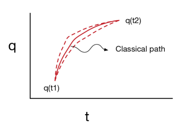
Figure 1: Sum over paths from $q(t1)$ to $q(t2)$

The easiest way to understand the notion of phases and statistics under exchange of particles in quantum mechanics is to think about how particles move around each other and from this point of view, the easiest way of understanding the quantum motion of these particles is via path integrals. Here, we will assume that you have some familiarity with the idea of path integrals, although not many details will be required. To recollect it, we just mention the following few things. In quantum mechanics, the probability amplitude to go from one space-time point to another is given by

$$A=\sum_{paths}e^{i\mathcal{S}}~{},$$ (1)

where $\mathcal{S}=\int\mathcal{L}dt$ is the action for the particular trajectory or path. In other words, quantum mechanically, we need to include all possible paths between the initial and final points of the trajectory sSee Fig.1). But most of these paths will interfere destructively with each other and hence will not contribute to the probability amplitude. The only exception is the classical path and the paths close to it, which interfere constructively with the classical path - i.e., the most important contribution will be from the classical path. That is all the information that we need here.

With this introduction, we come to the details of what we will study here. In Sec.(II), we will explain the basic notions of anyon physics and why they can exist only in two spatial dimensions. We will analyse a simple physical model of an anyon and use it to understand the quantum mechanics of two anyons and see that even in the absence of any interactions, it needs to be studied as an interacting theory, with the interactions arising due to the anyonic exchange statistics. Then, in Sec.(III), we will study the exactly solvable toric code model as an example of a system with anyonic excitations. Finally, in Sec.(IV), we will discuss non-abelian statistics, where again, we will explain many features of non-abelian anyons using the one-dimensional Kitaev model as a typical example.

II Abelian anyons

II.1 Basic concepts of anyon physics

The term ‘exchange statistics’ refers to the phase picked up by a wave-function when two identical particles are exchanged. But this definition is slightly ambiguous. Does statistics refer to the phase picked up by the wave-function when all the quantum numbers of the particles are exchanged (i.e., under permutation of the particles) or the actual phase that is obtained when two particles are adiabatically transported giving rise to the exchange? In three dimensions, these two definitions are equivalent but not in two dimensions. In quantum mechanics, we deal with interference of paths of particles and hence, it is the second definition which is more relevant, and we will show how it can be different from the first definition.

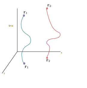
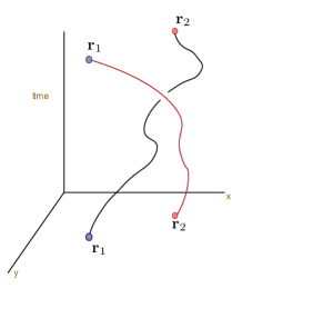
Figure 2: Direct and exchange paths

Let us first consider the statistics under exchange of two particles in three dimensions. By the path integral prescription, the amplitude for a system of particles that moves from (${\bf r}_{1}(t_{1}),{\bf r}_{2}(t_{1})$) to (${{\bf r}_{1}}^{\prime}(t_{2}),{{\bf r}_{2}}^{\prime}(t_{2})$) is given by

$$A=\sum_{paths}e^{i\int_{t_{1}}^{t_{2}}dt\mathcal{L}[{\bf r}_{1}(t),{\bf r}_{2}(t)]}~{}.$$ (2)

If the two particles are identical, then there are two classes of paths (see Fig.2). How do we see this? If we use the convention that we always refer to the position of the first particle first and the second particle second, then we see that the final configuration remains the same whether we have (${{\bf r}_{1}}(t_{2}),{{\bf r}_{2}}(t_{2}$)) or (${{\bf r}_{2}}(t_{2}),{{\bf r}_{1}}(t_{2})$) because the two particles are identical. Even though the particles are exchanged in one path and not in the other, the final configuration is the same. In terms of the centre of mass (${\bf R}=({\bf r}_{1}+{\bf r}_{2})/2$) and relative coordinates (${\bf r}={\bf r}_{1}-{\bf r}_{2}$), we see that the centre of mass motion is the same for both the paths, but the relative coordinate changes for both the paths. Also, since the CM motion moves both the particles together, it is independent of any possible phase under exchange. For convenience in visualising the configuration space, let us keep $|{\bf r}|$ fixed and non-zero, i.e, the two particles do not intersect. Then, the vector ${\bf r}$ takes values on the surface of the sphere.

Figure 3: Paths in three dimensional configuration space with fixed radius

Now let us draw the paths in configuration space as shown in Fig.3. It is clear that the paths can only move along the surface of the sphere as the two particles move, since $|{\bf r}|$ is fixed. But once they get back to their original positions or get exchanged, since they are indistinguishable, the path is closed. In other words, closed paths on the surface of the sphere are formed by the particles coming back to their original positions (no exchange) or going to the antipodal point (${\bf r}\rightarrow-{\bf r}$ or getting exchanged). But if we exchange the particles another time, then $\bf r$ comes back to itself, after having gone around the sphere once. In terms of diagrams, this is shown in Fig.13. Since we have eliminated coincident points, the wave-function is non-singular and well-defined at all points in the configuration space, and consequently on the surface of the sphere. So the phase picked up by the wave-function is also well-defined and does not change under continuous deformations of the path. Let us consider the possible phases of the wave-function when the motion of the particles is along each of the three paths, - A (no exchange), B (single exchange) and C (two exchanges) - depicted in Figs. 3(a),(b) and (c). Path A is a closed path which does not involve any exchange and can clearly be shrunk to a point. Hence, the wave-function cannot pick up any phase other than unity. Path B involves the exchange of the two particles and goes from a point on the sphere to its diametrically opposite point. Since the two end points are fixed, this path cannot be shrunk to a single point. So this exchange can have a non-trivial phase in the wave-function . However, path C which forms a closed loop on the surface and involves two exchanges can be continuously shrunk to a point by imagining the path to be a physical string looped around a sphere. So this again cannot pick up any phase. Let $\eta$ be the phase picked up under a single exchange. Since two exchanges are equivalent to no exchange, $\eta^{2}=+1\Longrightarrow\eta=\pm 1$. Hence, the only statistics possible in three dimensions are Fermi statistics or Bose statistics.

With slightly more mathematical rigour, one can say that the configuration space of relative coordinates is given by $({\mathbb{R}}_{3}-origin)/\mathbb{Z}_{2}$. Here ${\mathbb{R}}_{3}$ is just the three dimensional Euclidean space spanned by the relative coordinate ${\bf r}$. We subtract out the origin because we have assumed that paths do not cross (which is true for all particles other than bosons, because of hard core repulsion and for bosons, is not relevant anyway, because the exchange phase is unity). The division by ${\mathbb{Z}}_{2}$ is because of the identification of ${\bf r}$ with $-{\bf r}$, which is because the particles are indistinguishable. To study the phase picked up by the wave-function of a particle as it goes around another particle, we need to classify all paths in this configuration space. The claim, from the pictorial analysis above, is that there are just two classes of paths. Mathematically, this is expressed in terms of the first homotopy group $\Pi_{1}$ of the space, which is the group of inequivalent paths (paths not deformable to each other), passing through a given point in the space, with group multiplication being defined as traversing paths in succession and group inverse as traversing a path in the opposite direction. Thus

$$\Pi_{1}(\mathbb{R}_{3}-origin)/\mathbb{Z}_{2})=\Pi_{1}(\mathbb{RP}_{2})=Z_{2}$$ (3)

where $\mathbb{RP}_{2}$ stands for real projective space and is the notation for the surface of the sphere with diametrically opposite points identified and $\mathbb{Z}_{2}=(1,-1)$ is a group of just two elements.

Now that we have determined that there are two classes of paths in three dimensions, in terms of path integrals, the amplitude can be written as

$$A[{\bf r}_{1}(t_{1}),{\bf r}_{2}(t_{1}))\rightarrow({{\bf r}_{1}}^{\prime}(t_{2}),{{\bf r}_{2}}^{\prime}(t_{2})]=\sum_{direct~{}paths}e^{i\mathcal{S}}+\sum_{exchange~{}paths}e^{i\mathcal{S}}~{}.$$ (4)

The direct paths involve all closed paths which end at the same point and the exchange paths involve all paths which end on antipodal points, (which are also closed paths). In terms of the path integral, we can also introduce a phase between the two classes of paths and write

$$A[{\bf r}_{1}(t_{1}),{\bf r}_{2}(t_{1}))\rightarrow({{\bf r}_{1}}^{\prime}(t_{2}),{{\bf r}_{2}}^{\prime}(t_{2}))]=\sum_{direct~{}paths}e^{i\mathcal{S}}+e^{i\phi}\sum_{exchange~{}paths}e^{i\mathcal{S}}~{}.$$ (5)

Since have already seen that exchanging the particle twice leads again to the direct path, it is clear that $e^{2i\phi}=1$, which implies that $\phi$ can only be $0,\pi$ giving rise, as before, to bosons and fermions.

Figure 4: Paths in two dimensional configuration space with fixed radius

What changes in two dimensions? The point is that the topology of the configuration space is now different. In two spatial dimensions, the configuration space of the relative coordinates is given by $(\mathbb{R}_{2}-origin)/\mathbb{Z}_{2}$. Just as before, for ease of visualisation, we shall keep the magnitude of the relative coordinate fixed, so that configuration space can be represented by a circle, and since the particles are indistinguishable, diametrically opposite points are identified (see Figs.4(a),(b),(c)). Here, however, several closed paths are possible. The path A that involves no exchanges can obviously be shrunk to a point, since it only moves along the circle and back. But path B that exchanges the two particles is non-contractible since the end-points are fixed. But even path C, where both the solid and dashed line are followed in the clock-wise direction (or anti-clockwise direction) cannot be contracted to a point. This is easily understood by visualising the paths as physical strings looping around a cylinder. Thus, if $\eta$ is the phase under single exchange, $\eta^{2}$ is the phase under two exchanges, $\eta^{3}$ is the phase under three exchanges and so on. All we can say is that since the modulus of the wave-function remains unchanged under exchange, $\eta$ has to be a phase - $\eta=e^{i\theta}$. This explains why we can get ‘any’ statistics in two dimensions.

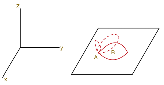
Figure 5: Path of A around B being lifted off the surface and shrunk to a point

The distinction between the paths in two and three dimensions can also be seen as follows. In three dimensions, the loop that is formed by taking a particle all around another particle (two exchanges) can be lifted off the plane and shrunk to a point as shown in Fig.5. This is not possible if the motion is restricted to a plane, as long as we disallow configurations where two particles are at the same point (removal of the origin).

The mathematical crux of the distinction between configuration spaces in two and three dimensions, is that the removal of the origin in two dimensional space, makes the space multiply connected (unlike in three dimensional space, where removal of the origin keeps it singly connected). So it is possible to define paths that wind around the origin. Mathematically, we can say that

$$\Pi_{1}((\mathbb{R}_{2}-origin)/\mathbb{Z}_{2})=\Pi_{1}(\mathbb{RP}_{1})=\mathbb{Z}$$ (6)

where $\mathbb{Z}$ is the group of integers under addition. $\mathbb{RP}_{1}$ is just the notation for the circumference of a circle with diametrically opposite points identified. The different paths are labelled by integer winding numbers.

So in terms of path integrals, we now see that paths starting and ending at the same positions (upto exchanges due to indistinguishability) can be divided into an infinite number of classes, all distinct. So we can write the total amplitude as

$$A=\sum_{direct~{}paths}e^{i\mathcal{S}}+e^{i\phi}\sum_{single~{}exchange}e^{i\mathcal{S}}+e^{2i\phi}\sum_{two~{}exchanges}e^{i\mathcal{S}}+\dots$$ (7)

where $\phi=0,\pi$ give the usual bosons and fermions, but since in general, $e^{in\phi}\neq 1$ for any $n$, $\phi$ can be anything and as we said earlier, ‘any’ statistics are possible in two dimensions.

Note that if we do want to understand exchange of particles in the Hamiltonian formulation without invoking path integral ideas, we need to pin down the particles by using a confining potential - $i.e.$, by putting them in a box -

$$H=\sum_{i}\frac{{\bf p}_{i}^{2}}{2m}+\sum_{i}V_{\rm box}({\bf x}_{i}-{\bf R}_{i})$$ (8)

The particles can now be moved around by changing ${\bf R}_{i}$ as a function of time. Since the particles are identical, exchanges are equivalent to closed paths, and do not depend on the geometry of the paths ${\bf R}_{i}(t)$ involved. So the statistics of the particles under exchange can be found by computing the Berry phase when the particles are exchanged. However, in this review, we shall basically use the path integral formalism.

II.2 Anyons obey braid group statistics

The distinction between the phase of the wave-function when the quantum numbers of the particles are exchanged and the phase obtained under adiabatic transport of particles should now be clear. Under the former definition, the phase $\eta^{2}$ after two exchanges is always unity, whereas the phase under the latter definition has many more possibilities at least in two dimensions. Mathematically, the first definition classifies particle under the permutation group $\mathbb{P}_{N}$, whereas the second one classifies particles under the braid group $\mathbb{B}_{N}$. The permutation group $\mathbb{P}_{N}$ is the group formed by all possible permutations of $N$ objects with group multiplication defined as successive permutations and group inverse as undoing the permutation. It is clear that permuting two objects twice brings the system back to the original configuration. Thus particles that transform as representations of the permutation group can only be bosons or fermions.

Figure 6: Elements of the braid group $\mathbb{B}_{4}$

On the other hand, when we adiabatically exchange two particles, we can visualise the process as paths in space-time with time being the vertical axis and space being the horizontal axis as shown in Fig.2. The particles can circle around each other and form closed paths by coming back to their original positions (upto permutations of the positions). The adiabatic exchange of particles classifies particles under the braid group. As we saw earlier, even under adiabatic exchange, in three spatial dimensions, we only have fermions or bosons, whereas in two dimensions, there are many other possibilities. Formally, the braid group $\mathbb{B}_{N}$ is the group of inequivalent paths that occur when adiabatically transporting $N$ particles. Since they represent a configuration of $N$ particles, at some particular time (say $t=0$), evolving to a configuration of $N$ particles at some later time $t=T$, the world lines cannot cross each other or form knots around each other or loop back. At each time, we want to have only $N$ particles. Each history or set of trajectories of the $N$ particles becomes a braid. For example, in Fig.6, we show an example of some elements of the braid group $\mathbb{B}_{4}$, which is the braid group of 4 particles. Exchanges of neighbouring particles (by some counting rule, since the particles are in two dimensional space) form the generators of the group. For instance, the generators of the group $\mathbb{B}_{4}$ are given in Fig.7 and are denoted as $\sigma_{j}$, $j=1,2,3$. $\sigma_{j}$ describes exchange of $j^{th}$ particle with $(j+1)^{th}$ particle in a counter-clockwise direction (by definition), so that the clockwise exchange is denoted by $(\sigma_{j})^{-1}$. The identity element is given by $\sigma_{0}$ where there is no exchange, and group inverse by the clockwise exchange $(\sigma_{j})^{-1}$ as shown in Fig.8. Group multiplication is defined as following one trajectory by another in time as shown in Fig.9. Note that we have put crosses on the time-lines which are identified (are at equal times) in the figure. It is now easy to check that $(\sigma_{j})(\sigma_{j})^{-1}=\sigma_{0}$ as shown in Fig.10 (without the crosses). It is also easy to see that $(\sigma_{1})^{n}\neq\sigma_{0}$ for any $n$, which is the reason that ‘any’ statistics are allowed in two dimensions. (See Fig.11).

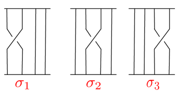
Figure 7: The three generators of the braid group $\mathbb{B}_{4}$

Figure 8: The identity and the inverse of the generator $\sigma_{1}$.

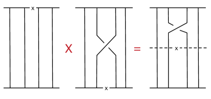
Figure 9: Group multiplication.

Figure 10: Product of $\sigma_{1}$ and $(\sigma_{1})^{-1}$ giving rise to identity.

Figure 11: $(\sigma_{1})^{n}\neq\sigma_{0}$

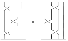
Figure 12: Yang-Baxter relations.

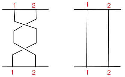
Figure 13: Different elements of the braid group, but same element of the permutation group.

We will end this subsection by mentioning the two defining relations satisfied by the generators of the braid group.

$$\sigma_{i}\sigma_{j}=\sigma_{j}\sigma_{i},\quad|i-j|\geq 2$$

$$\sigma_{j}\sigma_{j+1}\sigma_{j}=\sigma_{j+1}\sigma_{j}\sigma_{j+1}$$ (9)

The second one is called the Yang-Baxter relation. Both these relations can be easily checked pictorially ( as we show in Fig.12 for the generators of $\mathbb{B}_{4}$).

It should be clear by now that the braid group leads to a much finer classification than the permutation group. For instance, the two elements shown in Fig.13 are different elements of the braid group, but the same element of the permutation group. So the quantum theory of anyons has the quantum states of the anyons transforming as unitary representations of the braid group. Abelian anyons form one-dimensional representations of the braid group. There are an infinite number of such representations, because under exchange, the phase that is picked up is $e^{i\theta}$ and $\theta$ can take any value. $\theta=0$ and $\theta=\pi$ represent bosons and fermions respectively. We will discuss non-abelian representations in the last section.

II.3 Spin of an anyon

Let us start with spin in the familiar three dimensional world. We know that spin is an intrinsic angular momentum quantum number that labels different particles. The three spatial components of the spin obey the commutation relations given by

$$[S_{i},S_{j}]=\epsilon_{ijk}S_{k}$$ (10)

We shall show that these commutation relations constrain the spin to be either integer or half-integer. Let $|s,m>$ be the state with $S^{2}|s,m>=s(s+1)|s,m>$ and $S_{z}|s,m>=m|s,m>$. By applying the raising operator, we may create the state

$$S^{+}|s,m>=[s(s+1)-m(m+1)]^{1/2}|s,m+1>=|s,m^{\prime}>$$ (11)

Requiring this state to have positive norm for all $m$, leads to $m<s$. Thus, it is clear that for some integer $m^{\prime}=m+$integer, $m^{\prime}>s$ unless $s=m^{\prime}$ or

$$s-m={\rm integer}$$ (12)

Similarly by insisting that $S^{-}|s,m>$ have a positive norm, we get $s(s+1)-m(m-1)\geq 0$, which implies that $m\geq-s$ for all $m$. Once again, to avoid $m<-s$, we need to set

$$m-(-s)={\rm integer}$$ (13)

Adding the equations in Eqs.12 and 13, we get

$$2s={\rm integer}\Longrightarrow s={\rm integer}/2~{}.$$ (14)

Thus, just from the commutation relations, we can prove that the particles in three dimensions have either integer or half-integer spin.

However, in two dimensions, there exists only one axis of rotation, perpendicular to the plane of the two dimensions. Hence, here spin only refers to $S_{3}$ which has no commutation relations to satisfy, and hence it can be anything!

II.4 Physical model of an anyon

Now let us construct a simple physical model of an anyonwilczek . Imagine a spinless particle of charge $q$ orbiting around a thin solenoid along the $z$-axis at a distance ${\bf r}$ as shown in Fig14. When there is no current through the solenoid, the orbital angular momentum of the charged particle is quantitized as an integer - $l_{z}$ = integer. When a current is turned on, the particle feels an electric field that can easily be computed using

$$\int(\nabla\times{\bf E})d^{2}{\bf r}=\int Bd^{2}{\bf r}=-\frac{\partial\phi}{\partial t}$$ (15)

where $\phi$ is the total flux through the solenoid. This is just the Aharanov-Bohm effect. Hence,

$$\int{\bf E}\cdot d{\bf l}=2\pi|{\bf r}|E_{\theta}=-{\dot{\phi}}\quad{\rm leading~{}to}\quad{\bf E}=-\frac{{\dot{\phi}}}{2\pi|{\bf r}|}({\hat{z}}\times{\bf r})~{}.$$ (16)

Thus, the angular momentum of the charge particle changes with the rate of change given being proportional to the torque - i.e.,

$${\dot{l}_{z}}={\bf r}\times{\bf F}={\bf r}\times q{\bf E}=-\frac{q{\dot{\phi}}}{2\pi}\quad{\rm leading~{}to}\quad\Delta l_{z}=-\frac{q{\phi}}{2\pi}.$$ (17)

Thus $\Delta l_{z}$ is the change in the angular momentum due to the fiux in the solenoid. In the limit where the solenoid becomes very narrow and the distance between the charged particle and the solenoid is shrunk to zero, the system may be considered as a single composite object - a charge-fluxtube composite. In fact in a planar system, there is no extension in the $z$ direction. So this essentially point-like composite object with fractional angular momentum can be considered as a model of an anyon. Note that we have denoted this angular momentum as the change in the angular momentum due to the flux. So if we start with the original charge to be spinless, then the spin of the composite particle is given by $l_{z}=s_{z}=q\pi/2\pi$. This is also sometimes referred to as a topological spin and is intrinsic to the anyon. However, this is a little too naive. In an anyon, the charge and the fiux it carries are related - the charge gets turned on along with the flux. This implies that the $q$ in Eq.17 is time-dependent, and $q(t)=c\phi(t)$ for some constant $c$. Hence, we find

$$\Delta l_{z}=\frac{c\phi^{2}}{4\pi}=\frac{q\phi}{4\pi}$$ (18)

so that the angular momentum of a charge-flux composite with charge proportional to flux is less than what we originally computed by a factor of 1/2. In the next subsection, we shall see that it has the right statistics, and complete the identification of the charge-fluxtube composite as an anyon.

Figure 14: Physical model of an anyon.

II.5 Two anyon quantum mechanics

We shall now study the quantum mechanics of two anyons in order to determine its statistics using the simple physical picture of the anyon that we developed in the last subsection. The Hamiltonian for the system is given by

$$H=\frac{({\bf p}_{1}-q{\bf a}_{1})^{2}}{2m}+\frac{({\bf p}_{2}-q{\bf a}_{2})^{2}}{2m}$$ (19)

with

$${\bf a}_{1}=\frac{\phi}{2\pi}\frac{{\hat{z}}\times({\bf r}_{1}-{\bf r}_{2})}{|{\bf r}_{1}-{\bf r}_{2}|^{2}},\quad{\rm and}\quad{\bf a}_{2}=\frac{\phi}{2\pi}\frac{{\hat{z}}\times({\bf r}_{2}-{\bf r}_{1})}{|{\bf r}_{1}-{\bf r}_{2}|^{2}}$$ (20)

where ${\bf a}_{1}$ and ${\bf a}_{2}$ are the vector potentials at the positions of the composites (anyons) 1 and 2 due to the fluxes in composites (anyons) 2 and 1 respectively. Let us now work in the centre of mass (CM) and relative (rel) coordinates - i.e., we define respectively

$${\bf R}=\frac{{\bf r}_{1}+{\bf r}_{2}}{2}\Rightarrow{\bf P}={\bf p}_{1}+{\bf p}_{2},\quad{\rm and}\quad{\bf r}={\bf r}_{1}-{\bf r}_{2}\Rightarrow{\bf p}=\frac{{\bf p}_{1}-{\bf p}_{2}}{2}~{}.$$ (21)

In terms of these coordinates, the Hamiltonian can be recast as

$$H=\frac{{\bf P}^{2}}{4m}+\frac{({\bf p}-q{\bf a})^{2}}{m}\quad{\rm with}\quad{\bf a}_{rel}=\frac{\phi}{2\pi}\frac{{\hat{z}}\times{\bf r}}{|{\bf r}|^{2}}~{}.$$ (22)

Thus the CM motion which translates both the particles rigidly and is independent of the statistics is free. The relative motion, on the other hand, which is sensitive to whether the particles are bosons, fermion or anyons, reduces to the problem of a single particle of mass $m/2$ orbiting around a flux $\phi$ at a distance ${\bf r}$. Since the composites have been formed of a bosonic charge orbiting around a bosonic flux, the wave -function of the two composite system has to be symmetric under exchange and the boundary condition is given by

$$\psi({\bf r}_{1},{\bf r}_{2})=\psi({\bf r}_{2},{\bf r}_{1})\Longrightarrow\psi_{rel}({\bf r})=\psi_{rel}(-{\bf r})\Longrightarrow\psi_{rel}(r,\theta+\pi)=\psi_{rel}(r,\theta)$$ (23)

where $\psi_{rel}$ is the wave-function of the relative piece of the Hamiltonian and ${\bf r}=(r,\theta)$ in cylindrical coordinates.

Now, let us perform a (singular) gauge transformation so that

$${\bf a}_{rel}\longrightarrow{\bf a}^{\prime}_{rel}={\bf a}_{rel}-\nabla\Lambda(r,\theta)\quad{\rm where}\quad\Lambda(r,\theta)=\frac{\phi}{2\pi}\theta~{}.$$ (24)

This gauge transformation is singular because $\theta$ is a periodic angular coordinate with period $2\pi$ and is not single-valued. In the primed gauge,

$$a^{\prime}_{rel,\theta}=a_{rel,\theta}-\frac{1}{r}\frac{\partial\Lambda}{\partial\theta}=\frac{\phi}{2\pi r}-frac{\phi}{2\pi r}=0,\quad{\rm and}\quad{a^{\prime}}_{rel,r}=a_{rel,r}-\frac{\partial}{\partial r}\Lambda=0-0=0,$$ (25)

i.e., the gauge potential vanishes completely and the Hamiltonian just reduces to

$$H=\frac{{\bf P}^{2}}{2m}+\frac{{\bf p}^{2}}{2m}$$ (26)

which is just the Hamiltonian of two free particles. However, in the primed gauge, the wave function of the relative Hamiltonian has also changed. It is now given by

$$\psi_{rel}^{\prime}(r,\theta+\pi)=e^{-iq\phi/2}\psi_{rel}(r,\theta)~{}$$ (27)

-i.e., the particles obey anyonic statistics. So the problem of two free anyons is equivalent to the problem of two interacting charge flux composites described by the Hamiltonian in Eq.19. The quantum mechanical problem can be solved - we need to go back to the boson gauge ( since we do not know how to solve quantum mechanics problems with non-trivial statistics) and write the Hamiltonian in terms of centre of mass (CM) and relative coordinates and note that the CM motion becomes free and the relative motion acquires an extra $q\phi/2m$ factor in the angular momentum term, thus adding to the centrifugal barrier. The radial part of the relative motion can then be identified as a Bessel equation. Thus the two anyon wave-function can be written as

$$\psi({\bf R},{\bf r})=\psi_{\rm CM}({\bf R})\psi_{\rm rel}({\bf r})=e^{i{\bf P}\cdot{\bf R}}e^{i(l+q\phi/2m)\theta}J_{|l+q\phi/2m|}(kr)$$ (28)

where ${\bf r}=(r,\theta)$. The two particle wave-function can be recast in terms of the original single particle coordinates - $i.e.$, $\psi(({\bf R},{\bf r})=\psi({\bf r}_{1},{\bf r}_{2})$. However, unless $q\phi/2m$ is either integer or half-integer, the two particle wave-function cannot be factorised into a product of two suitable one-particle wave-functions. Also, the energy levels of the two anyon system cannot be obtained as sums of one anyon energy levels. This is easier to see with discrete energy levels and so we will next solve the problem of two anyons in a harmonic oscillator potential.

The Hamiltonian for two anyons in a harmonic oscillator potential is given by

$$H=\frac{{\bf p}_{1}^{2}}{2m}+\frac{{\bf p}_{2}^{2}}{2m}+\frac{1}{2}m\omega^{2}{\bf r}_{1}^{2}+\frac{1}{2}m\omega^{2}{\bf r}_{2}^{2}~{}.$$ (29)

The problem can be separated into CM and relative coordinates in terms of which the Hamiltonian is given by

$$H=\frac{{\bf P}^{2}}{4m}+\frac{{\bf p}^{2}}{m}+m\omega^{2}{\bf R}^{2}+\frac{1}{4}m\omega^{2}{\bf r}^{2}~{}.$$ (30)

The problem can now be solved in terms of the cylindrical $(R,\Theta)$ and $(r,\theta)$ coordinates. The CM motion is independent of the statistics of the particles and one can simply find the energy levels as

$$E_{CM}=\omega(n+|L|+1)~{}.$$ (31)

The Hamiltonian for the relative motion can be solved in the same way, except that because of the phase under exchange, we need to go to the boson gauge, where there is a dependence on the statistical gauge field - $i.e.$, we have

$$H_{rel}\psi_{rel}=[\frac{({\bf p}-q{\bf a}_{rel})^{2}}{m}+\frac{1}{4}m\omega^{2}{\bf r}^{2}]\psi_{rel}=E_{rel}\psi_{rel}~{}.$$ (32)

In terms of the $(r,\theta)$ coordinates, we now find that the energy levels are given by

$$E_{rel}=\omega(n+|l+\alpha/\pi|+1).$$ (33)

Note that $\alpha=0$ and $\alpha=\pi$ give the usual energy levels for bosons and fermions respectively. Otherwise, they are given by

$$E_{j} = (2j+1+\alpha/\pi),\quad{\rm degeneracy~{}~{}factor}=j+1,$$

$$E_{j} = (2j+1-\alpha/\pi),\quad{\rm degeneracy~{}~{}factor}=j~{}.$$ (34)

Clearly, the levels are not equally spaced and the total energy of the two anyon system given by

$$E_{2anyons}=E_{CM}+E_{rel}=(2j+p+2\pm\alpha/\pi)\omega,\quad p,j={\rm integers}$$ (35)

is not a sum of the one particle levels $E=(n+1)\omega$, with $n=$ integer. Similarly, the two anyon wave function is also not a simple product of one anyon wave functions. We find that

$$\psi({\bf R},{\bf r}) = e^{-m\omega(R^{2}+r^{2}/4)}r^{\alpha/\pi}e^{i\alpha\theta/\pi}\implies\psi({\bf r}_{1},{\bf r}_{2})\propto e^{-m\omega(r_{1}^{2}+r_{2}^{2})/2}({\bf r}_{1}-{\bf r}_{2})^{\alpha/\pi}$$ (36)

which does not factorise into a product of two single particle wave-functions except when $\alpha=0,\pi$. This is why even a system of free anyons needs to be tackled as an interacting problem. For more details, see Ref.anyonprimer, .

II.6 Many anyon systems

Finally, we briefly mention what happens when we have many anyons. As we have seen above, even the two free anyon system is an interacting system because of the statistical interactions. Hence, any many anyon system needs to be treated as an interacting system, where each particle has long-range statistical interactions with each of the other particles.

Here, we will just mention one important concept of many anyon systems, which is that of fusion rules. A system which has anyons must have many types of anyons. If we have an anyon with statistics parameter $\theta$, then we can combine two such anyons or make a bound state of two such particles. What would be the statistics of the bound state? You may naively think that it should be $2\theta$. But that is not correct. One can see this by thinking of the anyon as a charge-flux composite in two ways. (1) In terms of angular momentum, we can add up the individual spins of the two anyons - $\theta/2\pi+\theta/2\pi=\theta/\pi$. But we also need to include the orbital angular momentum of the anyon pair. Normally, the orbital angular momentum is an integer because the wave-function of the two particle system is single-valued, if you take one particle around the other. But here, the counter-clockwise transport of one anyon around another in a full circle leads to the phase $e^{-2i\theta}=e^{i2\pi L}$ where $L$ is the orbital angular momentum. Now adding the spin and orbital angular momentum, we find that the total angular momentum is $\theta/\pi+\theta/\pi=2\theta/\pi=4\theta/2\pi$ which gives the statistics parameter as $4\theta$. (2) Here, we note that a single anyon exchange leads to a phase of $e^{i\theta}$. So when a two anyon molecule exchanges with another 2 anyon molecule, there are $2^{2}=4$ exchanges and hence the phase acquired will be $e^{4i\theta}$, which agrees with the total spin of the bound state as well.

Now, we can generalise this to say that more particles can be bound together to form new bound states or new types of particles. This is called fusion. The statistics parameter when $n$ such particles are bound together is given by $e^{in^{2}\theta}$. One can think of this new particle as an $n$-charge-$n$-flux composite. The formation of a different type of anyon by bringing together two anyons is called fusion. If we bring together an anyon and anti-anyon with opposite statistics parameter ( $\theta$ and $-\theta$), the result has statistics zero, which is equivalent to having no particles. The system with no particles (called the vacuum) is often denoted by the identity $I$. It is also called a trivial particle.

For abelian anyons, it is clear that if we bring together 2 anyons with statistics parameter $\theta$, they give rise to an anyon with statistics parameter $4\theta$ and in general $n$ such particles give rise to anyons with statistics parameter $n^{2}\theta$. But for non-abelian anyons, this is no longer true. There is no unique way of combining anyons to form new anyons and one can have different outcomes by bringing them together (just like two spin1/2 particles can be brought together to form spin 0 or spin1 particles). These are called fusion channels. The probability of the different outcomes is specified by a set of numbers which give rise to the fusion rules.

In the next section, instead of studying anyons abstractly as we have done in this section, we shall study an explicit lattice model, whose excitations turn out to be abelian anyons. We will come back to this later when we study non-abelian anyons.

III Toric code model as an example of abelian anyons

Let us begin this section, by first answering two questions - what is the toric code and why do we want to study it. The toric code is actually a spin model defined on a two dimensional lattice. It was engineered by Kitaevkitaevtc to be exactly solvable and to have low energy excitations that are anyonic. The reason that this model became so important was because it was shown by Kitaev that these anyons could be used, in principle, to perform fault tolerant quantum computation - fault tolerant because information could be stored in the fusion properties of anyons, which could not be destroyed by local perturbations. This model is thus, the prototypical concrete lattice model for many of the more abstract ideas of quantum computation.

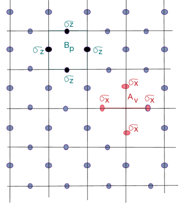
Figure 15: The Kitaev toric code model on a square lattice. Spins are placed on the links. The operator $A_{v}$ is the product of the $x$-components of the spin of the four links that cross at the vertex and the operator $B_{p}$ is the product of the $z$-component of the spins around the perimeter of the square.

III.1 Toric code on a square lattice

In general, the toric code model can be defined on any lattice, but here we will work on the simplest model which is an exactly solvable spin 1/2 model on a two dimensional square lattice of $N\times N$ pointskitaev2 ; burello . The spins are placed on the edges or links of an open lattice as shown in Fig.15 and it is easy to check that we have twice as many spins as the number of lattice points - $2N^{2}$. The components of the spins on different links commute with one another. On a given link, the spins satisfy the usual anti-commutation relations $\{\sigma_{\alpha},\sigma_{\beta}\}=2\delta_{\alpha\beta}$ where $\alpha,\beta=x,y,z$. The Hamiltonian for the model is given bykitaev2

$$H=-J_{e}\sum_{v}A_{v}-J_{m}\sum_{p}B_{p}$$ (37)

where

$$A_{v}=\Pi_{j\in v}\sigma_{j}^{x}~{}~{}{\rm and}~{}~{}B_{p}=\Pi_{j\in p}\sigma_{j}^{z}$$ (38)

are the vertex operator that acts on the four spins surrounding the vertex and the plaquette operator involving the four spins around the plaquette, respectively, as shown in Fig.15. Note that this is not a very common or physical looking Hamiltonian since it has four spin interactions, and has explicitly been engineered for a purpose! As can be easily seen from the diagram, every spin is a part of two vertex and two plaquette operators. The eigenvalues of both $A_{v}$ and $B_{p}$ are $\pm 1$. However, the product of the eigenvalues over all the plaquettes or all the vertices is always unity - i.e.,

$$\Pi_{j\in V}A_{V}=\Pi_{j\in P}B_{p}=+1$$ (39)

where $V=$ total number of vertices in the model is $N^{2}$ and $P=$ total number of plaquettes in the model is also $N^{2}$.

Note that the vertex operators contain the $x$-component of the spins and the plaquette operators contain the $z$-component of the spins. Hence, it is easy to check that the vertex operators and the plaquette operators commute among themselves

$$[A_{v},A_{v^{\prime}}]=[B_{p},B_{p^{\prime}}]=0$$ (40)

But it is also true that $[A_{v},B_{p}]=0$. This is trivially true if they do not have any spins in common, since spins on different sites commute. But in case, they do have a spin in common, they will always have two spins in common. For example, from Fig.16, it is clear that the plaquette $B_{\alpha_{1}}$ shares spins with the four vertex operators $A_{\beta_{1}},...A_{\beta_{4}}$. But with each of them, it shares 2 spins. For instance, we have

$$[B_{\alpha_{1}},A_{\beta_{1}}]=\sigma_{1}^{z}\sigma_{2}^{z}\sigma_{3}^{z}\sigma_{4}^{z}\sigma_{1}^{x}\sigma_{2}^{x}\sigma_{5}^{x}\sigma_{6}^{x}-\sigma_{1}^{x}\sigma_{2}^{x}\sigma_{5}^{x}\sigma_{6}^{x}\sigma_{1}^{z}\sigma_{2}^{z}\sigma_{3}^{z}\sigma_{4}^{z}$$ (41)

which is zero because $\sigma_{1}^{z}\sigma_{1}^{x}=-\sigma_{1}^{x}\sigma_{1}^{z}$ and $\sigma_{2}^{z}\sigma_{2}^{x}=-\sigma_{2}^{x}\sigma_{2}^{z}$. So the two negative signs cancel each other. The same thing goes through for the other three vertex operators as well. So the bottomline is that all the terms in the Hamiltonian commute with each other, and commute with the Hamiltonian. So all the $A_{v}$ and $B_{p}$ operators can be simultaneously diagonalised and their values can be used to label the states.

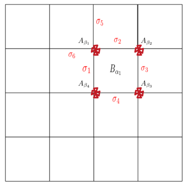
Figure 16: Commutation relations of the operators on different links and same links. See text for details.

The next step is to find the ground state of the Hamiltonian. This means that the energy of all the terms in the Hamiltonian have be minimised, which, in turn means that each of the $A_{v}$ and $B_{p}$ terms have to be maximised. Let us work in the $\sigma_{z}$ diagonal basis. The eigenvalues of $\sigma_{j}^{z}$ are $s_{j}=\pm 1$. Let us also define $\omega_{p}(s)$ , the product of the eigenvalues around the plaquette $p$ (where $s$ stands for the configuration of $\{s_{j}\}$). This can also be just +1 or $-1$. We will call this the flux through the plaquette. A configuration where $\omega_{p}=-1$ is called a vortex (or flux) configuration. (See Fig.17 for examples.) Now suppose that we have only $B_{p}$ terms in the Hamiltonian - i.e. $H=-J_{m}\sum_{p}B_{p}$. Here, again the only possible eigenvalues for the operator $B_{p}$ are +1 and $-1$ and the configurations are all given in Fig.17. We note that there are eight configurations with ‘no flux’ ($\omega_{p}=+1$) and eight configurations with non-zero flux (vortex configurations with $\omega_{p}=-1$) as shown in Fig.17. As to why these are called flux configurations, it turns out that this toric code model turns out to be the same as the $Z_{2}$ gauge theory on a lattice, and the flux is that of the $Z_{2}$ gauge field. But the study of this connection is beyond the scope of these lectures and for us here, the word flux can be thought of as just nomenclature. The ground state is now clearly given by any linear combination of configurations which have no vortices -i.e, the ground state is given by

$$|\psi>=\sum_{\{s,\omega_{p}(s)=+1\forall p\}}C_{s}|s>$$ (42)

where $C_{s}$ is arbitrary. All we know about the ground state is that it has no vortices and

$$B_{p}|\psi>=|\psi>~{}~{}\forall~{}B_{p}$$ (43)

because the eigenvalue of $B_{p}$ acting on $|s>$ is always $+|s>$. For $2N^{2}$ spins, the ground state degeneracy would be $2^{N^{2}}$ (because pairs have to be either $\uparrow$ or $\downarrow$). In other words, of the total number of configurations $2^{2N^{2}}$, $2^{N^{2}}$ would have $\omega_{p}=+1$ ( ground state configuration) and $2^{N^{2}}$ would have $\omega_{p}=-1$ ( vortex configuration).

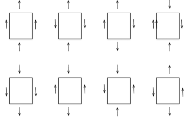
Figure 17: The configurations of spins on each plaquette on the left have $\omega_{p}(s)=1$ and the configurations on the right have $\omega_{p}(s)=1$

Now let us add back the vertex terms to the Hamiltonian. The $A_{v}$ acts on $|s>$ by flipping spins, since $\sigma_{x}\sigma_{z}\sigma_{x}^{-1}=-\sigma_{z}$, but in any plaquette, it will always flip two spins. So it will keep configurations with $\omega_{p}=1$ in configurations with $\omega_{p}=1$. Hence, operation of $A_{v}$ on $|s>$ will only take it to some other $|s^{\prime}>$, which will also belong to the same set of vortex free configurations with $\omega_{p}(s)=1$. But since $A_{v}$ can act on any of the lattice points, $A_{v}$ can be an eigen-operator for $|\psi>$ only if $C_{s}=+1$ for all $s$. So now, we define

$$|\Psi_{0}>=\sum_{\{s,\omega_{p}(s)=+1\forall p\}}|s>$$ (44)

as the ground state with all $A_{v}$ and $B_{p}$ acting on it with eigenvalue 1. (We could have worked in a $\sigma_{x}$ diagonal basis, and defined a state $|s^{\prime}>$ with ‘no ($x$) vortices’ in the dual lattice configuration so that $A_{v}$ acting on the state would give +1 for all $v$ and repeated the same argument. So it is clear that this ground state is a sum over all spin configurations that have neither $x$ nor $z$ ‘vorticity’.) It has an energy $E=-2N^{2}J_{e}-2N^{2}J_{m}$. Any excitation over this ground state must have non-zero vorticity which would imply that at least one of the spins would have to flip in either the $z$ or $x$ directions. In that case, 2 of the $B_{p}$’s or 2 of the $A_{v}$’s would have eigenvalues $-1$ and hence, the energy of the excitation would be either $4J_{m}$ or $4J_{e}$, but we will come back to these excitations later.

So we have found the ground state of an interacting Heisenberg spin model in two dimensions exactly, essentially because the Hamiltonian has been constructed to be exactly solvable. The ground state can also be written as

$$|\Psi_{0}>=N\prod_{v}(1+A_{v})|\xi>$$ (45)

where $|\xi>$ is some reference state. For example, we can take $|\xi>$ to be the state with all spins pointing $\uparrow$. The easiest way to check that this is the ground state is to check that for all $A_{v}$ and $B_{p}$, we get the eigenvalue +1, when they act on this state. Let us check this.

$$A_{v^{\prime}}|\Psi_{0}>=A_{v^{\prime}}N\prod_{v}(1+A_{v})|\xi>$$ (46)

First consider the terms where $v\neq v^{\prime}$. Then $A_{v^{\prime}}A_{v}=A_{v}A_{v^{\prime}}$. But for $v=v^{\prime}$, $A_{v^{\prime}}(1+A_{v^{\prime}})=A_{v^{\prime}}+1$, since $A_{v^{\prime}}^{2}=1$. Hence

$$A_{v^{\prime}}|\Psi_{0}>=+1|\Psi_{0}>$$ (47)

Furthermore, we already know that $A_{v}$ acting on any state does not change its $z$-vorticity since it always flips two spins. Since the reference state has vorticity = +1 and $B_{p}=+1$ on all states with vorticity =+1, we also have

$$B_{p}|\Psi_{0}>=+1|\Psi_{0}>~{}.$$ (48)

This is essentially a unique ground state on a plane or with open boundary conditions. We shall see later what happens when we have periodic boundary conditions which is equivalent to putting the model on a torus. But before that, let us see how to create excitations over the ground state.

III.2 Excitations over the ground state and fusion rules

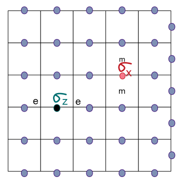
Figure 18: Flipping the $z$-component of the spin by $\sigma_{x}$ creates 2 monopoles, in adjacent plaquettes whereas flipping the $x$-component of the spin by $\sigma_{z}$ creates 2 charges at adjacent vertices.

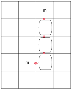
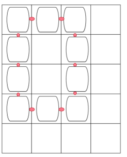
Figure 19: (a) A pair of monopoles created by flipping the $z$-component of the spin by $\sigma_{x}$ along a string on the dual lattice. (b) Annihilating the monopoles by closing the string. This configuration again has zero vorticity and commutes with the Hamiltonian. (Note that the spins that do not change are not shown in this diagram and in most further diagrams, where they are obvious, in the interest of not cluttering the diagrams.)

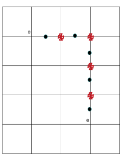
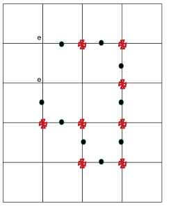
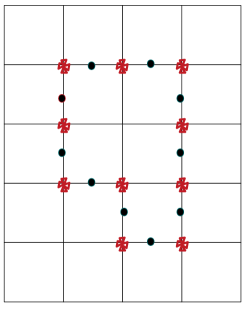
Figure 20: (a) A pair of electric charges created by flipping the $x$-component of the spin by $\sigma_{z}$ along a string. Note that the vertices in between the spins all have spins flipped on two links connected to them. (b) Moving one of the charges by flipping more spins and increasing the length of the string (c) Annihilating the charges by closing the string. This configuration has zero vorticity and commutes with the Hamiltonian.

There are two types of excitations that we can create on the ground state - one by applying $\sigma_{x}$ and the other by applying $\sigma_{z}$. Another way of thinking about excitations is to note that both $A_{v}$ and $B_{p}$ acting on the ground state have eigenvalues +1. One can make excitations if any of these values for some vertex or some plaquette becomes $-1$. First, let us try to make the vorticity in a given plaquette become $-1$. To do this, we need to flip the $z$-component of the spin on one link, which can be done by applying $\sigma_{x}^{i}$ on the $i^{th}$ link. So $\sigma_{x}^{i}|\Psi>$ flips $\uparrow$ to $\downarrow$ on the $i^{th}$ spin. However, this gives the value for $B_{p}$ to be $-1$ on two plaquettes, since the link is common to two plaquettes. The energy of this excitation is clearly $2J_{m}+2J_{m}=4J_{m}$ since the sign change of a single plaquette costs $2J_{m}$. These excitations are shown in Fig.18 where 2 e-excitations have been created on neighbouring vertices and 2 m-excitations in neighbouring plaquettes.

Note that the the pairs of excitations can be moved away from one another at no cost in energy. This is most easily seen diagrammatically. The string $\Pi_{j\in t^{\prime}}\sigma_{x}^{j}$ between the two magnetic excitations (or monopoles) changes the $z$-component on all the links between the end points as shown in Fig.19(a), but essentially all the intermediate plaquettes have $B_{p}=+1$. If we consider drawing a line between the two monopoles, note that this line (or contour or string) is defined on the dual lattice.

Similarly, $A_{v}=-1$ if the $x$-component of the spin on one of the links gets flipped. This can be done by applying $\sigma_{z}$ to the ground state. But here again, the change of the $x$-component of the spin on a link affects two vertices, and hence creates a pair of electric excitations with energy $2J_{e}+2J_{e}=4J_{e}$. Once again, the two members of the pair of excitations can be moved away from one another at no cost in energy as is shown in Figs.20(a,b) by applying a string of operators, $\Pi_{j\in t}\sigma_{z}^{j}$ between the two electric excitations. Here if we draw a line between the e-excitations, the line or string is defined on the lattice. The string changes the eigenvalues of the $x$ components of all the spins belonging to the string. However, except at the end points of the string, every vertex will have two spins flipped and will continue to have $A_{v}=+1$. It is only at the two ends of the string, that the vertices will have $A_{v}=-1$. For instance in Fig.20(a), we have flipped the $x$-component of 5 spins. However, we have created only two electric excitations.

We can even make closed string loops that create, move and annihilate the electric or magnetic charges as shown in Figs.19(b) and 20(c). These loops have $z$ or $x$ vorticity =+1 - i.e., they commute with all $A_{v}$ and $B_{p}$. In other words, they commute with the Hamiltonian and can be thought of as symmetries, and the existence of these symmetries is the reason for the exact solvability of the model. The ground state can also be thought of as a superpositions of all these loops.

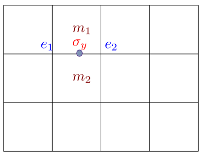
Figure 21: A pair of monopoles and a pair of electric charges created by flipping both the $x$-component and $z$-component of the spin by $\sigma_{y}$. This is equivalent to a pair of $\epsilon$ excitations.

Are there any other kind of excitations in the toric code? One might think that by applying $\sigma_{y}$ on the ground state, we may get new excitations. In fact, it turns out that there is a new excitation, which is a composite of the electric and magnetic excitations, which is called the $\epsilon$ excitation -

$$|\epsilon>=\sigma_{z}^{i}\sigma_{x}^{i}|\Psi_{0}>=i\sigma_{y}^{i}|\psi_{0}>$$ (49)

Essentially, $\sigma_{y}^{i}$ acting on a spin flips both its $\sigma_{x}$ and $\sigma_{z}$ components. So by applying it on a link as shown in Fig.21, it creates a pair of electric and magnetic excitations, or a pair of $\epsilon=e\times m$ excitations. There are no further excitations that can be created. So the particle content of the model is given by $I$ (no particles), $m$-particles, $e$-particles and $\epsilon=e\times m$-particles.

Now let us see what happens if we apply two $\sigma$ operators on the same plaquette. We know that $\sigma_{x}^{j}$ applied on a state creates a pair of excitations ( $m$- particles) on two adjoining plaquettes. But if we apply $\sigma_{x}^{i}$ twice, we do not get two pairs of excitations, because $(\sigma_{x}^{j})^{2}=I$ and $I$ operating on a state does not give rise to any excitation. So one cannot have more than one $m$-particles in each plaquette. This leads us to what are called fusion rules. We find that

$$e\times e = I$$ (50)

$$m\times m = I$$ (51)

$$\epsilon\times\epsilon = I~{}.$$ (52)

Further we had already seen that the first line of the following set of equations are true and it is not hard to check that the others are true as well -

$$e\times m = \epsilon$$ (53)

$$e\times\epsilon = m$$ (54)

$$m\times\epsilon = e~{}.$$ (55)

We had earlier seen that we can define string operators to move particles away from one another and even annihilate them by forming closed loops. We said that all these closed loops formed by creating, moving and annihilating particles, cost no energy and commute with the Hamiltonian. They are products of $A_{v}$’s or $B_{p}$’s and can be thought of as trivial symmetries of the Hamiltonian because they map the Hamiltonian onto itself. The ground state is unique and a linear combination of all these vortex-free states.

III.3 Toric code on a torus and topological degeneracy

Figure 22: Operators $W_{1\gamma_{1}}$ and $W_{2\gamma_{2}}$ which are defined by taking the product of the $z$ component of the spins, $\sigma_{z}^{j}$, along the paths $\gamma_{1}$ (red) going from top to bottom and $\gamma_{2}$ (cyan) going from left to right

But a new element is introduced if we have periodic boundary conditions or equivalently, consider the toric code model on a torus. In this case, there are two other independent operators, that we can define, which are not the products of the $A_{v}$ and $B_{p}$ operators of the Hamiltonian, and which can take the values $+1$ and $-1$. We can write them as

$$W_{1\gamma_{1}} = \prod_{j\in\gamma_{1}}\sigma_{z}^{j}$$ (56)

$$W_{2\gamma_{2}} = \prod_{j\in\gamma_{2}}\sigma_{z}^{j}$$ (57)

where $\gamma_{1}$ and $\gamma_{2}$ are paths which go from one edge of the torus to the other in the two orthogonal directions - for definiteness, let us assume that the loop $\gamma_{1}$ is in the vertical direction and the the loop $\gamma_{2}$ is in the horizontal direction - as shown in Fig.22. They form non-contractible loops. The paths can be moved around by multiplying the $W_{i}$’s with $B_{p}$’s, (because they do not change anything since they just give +1 on the ground state as shown in Fig.23). But there is precisely one non-contractible loop in each direction, which we can take to be the shortest path. It is easy to see that $W_{1}^{2}=W_{2}^{2}=1$ which says that $W_{1},W_{2}$ have eigenvalues $\pm 1$. They are symmetries, because they commute with the Hamiltonian. They also commute with one another and hence, they give rise to a four-fold degeneracy of the ground state -

$$|W_{1},W_{2}>_{gs}=|1,1>,~{}~{}|1,-1>,~{}~{}|-1,1>,~{}~{}|-1,-1>$$ (58)

because each of the $W_{i}$ can take values $\pm 1$.

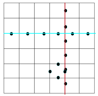
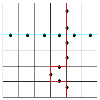
Figure 23: The operator $W_{1\gamma_{1}}$ can changed by multiplying the operator by $B_{p}$. This essentially changes the path $\gamma_{1}$, which is now no longer the straight vertical path.

Now let us show that this degeneracy is topological and there is no local operator that can cause transitions between these four ground states.

We shall first see if there are any operators that connect the degenerate states in the ground state manifold. We have already defined $W_{1}$ and $W_{2}$. Let us now define also

$$W_{3\gamma_{1}} = \prod_{j\in\gamma_{1}}\sigma_{x}^{j}$$ (59)

$$W_{4\gamma_{2}} = \prod_{j\in\gamma_{2}}\sigma_{x}^{j}$$ (60)

where $W_{3}^{2}=W_{4}^{2}=1$. These operators also commute with the Hamiltonian, but they do not increase the degeneracy, because as we shall see below, they do not commute with the earlier operators. There are only 4 mutually commuting operators that commute with the Hamiltonian. Clearly, $[W_{1},W_{2}]=0$ and $[W_{3},W_{4}]=0$. It is also easy to see that if both the loops are in the vertical or horizontal direction, they will commute, since they can always be displaced, i.e., we see that $[W_{1},W_{3}]=0$ and $[W_{2},W_{4}]=0$. However, this is not true when we consider $W_{1}$ and $W_{4}$. With even the simplest choice of path, they must have at least one spin in common, since one of the paths is vertical and the other horizontal. (More complicated paths will also always give odd number of common spins). So if this common spin is at location $0$, then it is the anticommutator of the two operators which vanishes - $\{W_{1},W_{4}\}=\{\sigma_{(0)}^{z},\sigma_{(0)}^{x}\}=0$ (and similarly $\{W_{2},W_{3}\}=0$). So it is as if we can define $W_{1}=\sigma_{1}^{z},W_{2}=\sigma_{2}^{z},W_{3}=\sigma_{2}^{x},W_{4}=\sigma_{1}^{x}$, so that the $W_{i}^{\prime}$s can be represented as Pauli matrices. Thus, $W_{3}$ and $W_{4}$ can change the eigenvalues of $W_{1}$ and $W_{2}$ by acting on the spins one at a time.

Now how do we confirm that the ground state degeneracy is a topological degeneracy and is topologically protected? The idea is that no local operator allows transitions between the different ground states. Suppose $\Omega$ is a local operator -i.e., it is of the form

$$\Omega\equiv\sigma_{i}^{\alpha}\sigma_{j}^{\beta}\sigma_{k}^{\delta}\dots$$ (61)

where the links $i,j,k$ are nearby in the sense that the maximum distance is small compared to the thermodynamic limit $N$. Then, we can always ensure that

$$[\Omega,W_{i}]=0$$ (62)

This means that $\Omega$ commutes with both $\sigma_{i}^{x}$ and $\sigma_{i}^{z}$ - i.e., with both Pauli matrices at a given site. This means that it has to be proportional to the identity. So it cannot directly cause any transition between different ground states. It can only lead to transitions if it can cause indirect transitions which will take it out of the ground state manifold. This would cost an energy $E_{0}$ which is the energetic distance to the next state. Moreover, since the operator is local, it would have to be applied $N$ times since the $W_{3,4}$ operators change the state of 1 link at a time. So if the relevant matrix element of $\Omega$ is $\omega$, we see that the total transition amplitude is of $O((\omega/E_{0})^{N})$ which goes to zero in the thermodynamic limit as long as $\omega/E_{0}<1$. In other words, no local operators can cause transitions between the degenerate states. One needs a non-local measurement to distinguish between the four degenerate ground states. This is why the ground state is said to have topological order, and this is what makes it relevant for quantum computation.

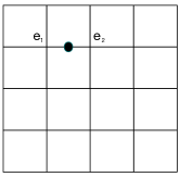
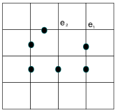
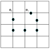
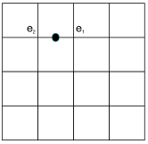
Figure 24: The exchange of the charges $e_{1}$ and $e_{2}$ by operating with the string operator $\Pi_{j}\sigma_{j}^{z}$. In the last step, we have simply removed a closed string loop of vorticity zero.

III.4 Statistics and braiding properties of the excitations

Finally, we want to understand the statistics and braiding properties of the excitations. Let us first look at the statistics of $e$-particles. $\sigma_{i}^{z}|\zeta>$, where $|\zeta>$ is the ground state, creates two $e$-particles in the adjacent vertices to the edge $i$. A string $\Pi_{j}\sigma_{j}^{z}$ can separate the two excitations. As shown in Fig.24, the two particles can even be exchanged by applying the string operators. But since all $\sigma^{z}$’s commute with one another, whichever way we move them, we do not get any phase. Thus, the $e$-excitations are bosons. Similarly, it is easy to argue that all $m$-excitations are also bosons.

But now let us see consider the mutual statistics between $e$ and $m$ particles. We first create pairs of $e$ and $m$ excitations at sites $i$ and $j$ by applying $\sigma_{i}^{z}\sigma_{j}^{x}|\zeta>$. We then separate the excitations by applying string operators as shown in Fig.25(a) and then we move an $e$-particle all around an $m$-particle, as shown in the series of figures in Fig.25(b), Fig.25(c) and Fig.25(d). It is clear that there is one site at which the $\sigma^{x}$ has to be taken beyond a $\sigma^{z}$ spin. This anti-commutation gives rise to a minus sign. The closed loop can be removed and the net effect of the process is that

$$\sigma_{i}^{z}\sigma_{j}^{x}|\zeta>\rightarrow-\sigma_{i}^{x}\sigma_{j}^{x}|\zeta>~{}.$$ (63)

Now let $R_{em}$ be the operator that exchanges the $e$ and $m$ particles. We have found that the wavefunction for the creation of the two excitations,

$$\psi({\bf r}_{e},{\bf r}_{m})\rightarrow R_{em}^{2}\psi({\bf r}_{e},{\bf r}_{m})=-\psi({\bf r}_{e},{\bf r}_{m})$$ (64)

since taking one particle completely around another is equivalent to two exchanges. Hence $R_{em}=e^{\pm i\pi/2}=\pm i$, which means that the $e$ and $m$ particles have mutual anyon statistics.

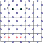
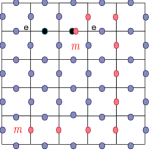
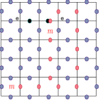
Figure 25: The sequence of steps in taking an $m$ charge around an $e$ charge by operating with the string operator $\Pi_{j}\sigma_{j}^{x}$. In the second step, we note that a $\sigma_{x}$ has to go past a $\sigma_{z}$, leading to a negative sign. In going from the third to the last figure, a closed loop of $\sigma_{x}$ operators has been removed, returning the configuration to the original configuration in the first figure.

We have already seen that $R_{ee}=R_{mm}=1$. The $e$ and $m$ particles are bosons under exchange. What about the $\epsilon$ particles? It is clear that if we take one $\epsilon$ particle completely around another, it is equivalent to taking an electron-monopole pair completely around another electron-monopole pair ( since $\sigma_{y}|g.s>\sim\sigma_{x}\sigma_{z}|g.s>$). In this case, the phase we expect to get is +1 since there will be two negative signs coming from anti commuting a $\sigma_{x}$ through a $\sigma_{z}$ and vice-versa, so two anti-commutations altogether. But this is not enough to tell us whether a single exchange gives a +1 or a -1. But the fact that taking the $m$ particle around the $e$ particle gives rise to a -1 can be interpreted as getting a negative sign when the $\epsilon$ particle is rotated through $2\pi$. This is the signature of a fermion. It is a ‘spinor’ and requires a rotation through $4\pi$ to get back to itself. Hence, the $\epsilon$ particle is a fermion and we conclude that $R_{\epsilon\epsilon}=-1$.

So now we have all the fusion and braiding rules for the excitations of the toric code. The particle content of the model is given by $I,e,m,\epsilon$. The fusion rules are

$$e\times e=I,~{}~{}~{}m\times m=I,~{}~{}~{}\epsilon\times\epsilon=I$$

$$e\times m=\epsilon,~{}~{}~{}e\times\epsilon=m,~{}~{}~{}m\times\epsilon=e$$ (65)

and the braiding rules are

$$R_{ee}=R_{mm}=1,~{}~{}~{}R_{\epsilon\epsilon}=-1,~{}~{}~{}R_{em}=i$$ (66)

Hence, this model has mutual (abelian) anyonic statistics. We will leave this model here and now go on to study a model which has non-abelian anyon statistics.

IV Non-abelian anyons

In this section, we will study a modelkitaev3 which has non-abelian anyon excitations. Let me start with a brief explanation of why non-abelian anyonsmooreread ; mong are of interest today, other than being an exotic form of exchange statistics. The reason is that they are expected to be relevant to quantum computationalicea . Quantum computation requires the possibility of storing quantum information. This needs a ‘protected’ portion of the Hilbert space which will not be disturbed by noise, temperature, etc, as long as the length scales are below the gap which separates the ‘protected’ states from the rest of the states. This protection may be due to some symmetry or even due to topology, which, in a sense acts like a robust symmetry, since it cannot be easily destroyed. This leads us to the idea of topological ordertopologicalorder , which exists if there is a degeneracy due to topology. For instance, in the earlier section, we studied the toric code, which had only abelian (mutual) anyons and no degeneracy on the plane. But the toric code on a torus has a four-fold degeneracy which was topological and could be used for quantum computation.

In general, in models with non-abelian anyons, we will find that the ground state is degenerate, and if the ground state is separated from all other states by a gap, then the ground state has topological order and can be used for quantum computation.

With this motivation, let us now seepreskill what one means by non-abelian excitations. Suppose we have $N$ degenerate states represented by $\psi_{\alpha}$ $,\alpha=1\dots N$, representing $N$ particles. The idea is that if we now exchange particles 1 and 2, it can now do more than just give a phase. It can rotate the state to another wave-function in the same degenerate space. In other words, the column vector $\psi=(\psi_{1}\psi_{2}\dots\psi_{N})^{T}\rightarrow\psi^{\prime}=U\psi$ where $U\equiv U_{\alpha\beta}$ is an $N\times N$ unitary matrix. If we now exchange two other particles, say 2 and 3, it could lead to $\psi\rightarrow\psi^{\prime}=V\psi$ with $V$ another unitary $N\times N$ matrix. If $U$ and $V$ do not commute, which, in general, they will not, the particles are said to have non-abelian statistics. Clearly, to have non-abelian statistics, we need to have at least 2 degenerate states, since otherwise, $U$ and $V$ are just phases and commute and we have abelian anyons.

One could think about generalising the physical model of any anyon - a charge orbiting around a flux - to the non-abelian case. In this case, the non-abelian charge would be a vector $|q_{i}>=\begin{pmatrix}q_{1}&q_{2}&.&.&q_{N}\end{pmatrix}$ moving around a non-abelian flux and returning to its original position, but in the process, instead of just acquiring phase factors,

$$|q_{i}>\rightarrow|q_{i}^{\prime}>=\sum_{j}U_{ij}|q_{j}>~{},$$ (67)

where $U_{ij}$ is the non-abelian flux matrix. But unlike the abelian flux which was path independent, the non-abelian counterpart $U$ is path dependent. It depends on where the path begins and ends as well as the contour. If we think of $U$ as a matrix belonging to the gauge group $U(N)$ or $SU(N)$, it means that the transport of charge around a flux is gauge dependent because $U$ depends on the choice of gauge. It is only the eigenvalues of $U$ (also called conjugacy class of the flux in group $G$) which is gauge independent. So for the non-abelian anyons, the physical picture does not help in simplifying or understanding the model and it is better to deal with the more abstract picture.

The main ingredients for a theory of non-abelian anyons are the following -
(1) We need a list of types of particles in the model.
(2) We need fusion rules - rules for fusing two constituents into one and also for splitting a particle into two constituents, which is its inverse.
(3) We need rules for braiding two particles (equivalently exchanging two particles).

Figure 26: The first denotes a local excitation, since it can be removed by flipping two spins locally, whereas the second one is a topological quasi-particle since it is protected by the boundary conditions which are fixed.

So let us now start with an abstract model. We first need a list of particles with their charges. Note that here by charges, we mean topological charges. In a condensed matter system, one can have quasi-particle excitations which are local or which are topological. For instance, in the toric code model that we studied in the last section, a spin operator could be applied locally (at a given position) to create a pair of excitations ($e$-type or $m$ type particles by applying $\sigma_{x}$ or $\sigma_{z}$). So a pair of excitations is a local or trivial type of particle or equivalent to the identity. But individually, the $e$ or $m$ particles carry a $Z_{2}$ charge which is topological. Another example is that of spin flip excitations in an Ising model as shown in Figs. 26(a) and 26(b). A single spin-flip (or even a few spin flips) is a local excitation and is equivalent to the identity as far as particle type is considered. But a domain wall is a topological excitation that is protected by the boundary conditions and cannot be removed by local perturbations. So let us list the topological particles in our system as $a,b,c,\dots$.

Next, we need to specify the fusion rules for these particles. The fusion algebra is defined as

$$a\times b=\sum_{c}N_{ab}^{c}c$$ (68)

where $N_{ab}^{c}\geq 1$. This equation simply means that if $N_{ab}^{c}=0$,then the particle $c$ is not obtained and if $N_{ab}^{c}=1$, then the particle $c$ is obtained as a fusion product and if $N_{ab}^{c}>1$, then $c$ can be obtained in $N_{ab}^{c}$ ways. Here, $a,b,c$ are just labels of the different kinds of particles. For abelian anyons, an anyon with statistics parameter $\alpha_{1}$ will fuse with an anyon with statistics parameter $\alpha_{2}$ to yield a specific anyon with statistics parameter $\alpha_{3}$ and $N_{\alpha_{1}\alpha_{2}}^{\alpha_{3}}=1$ and is otherwise zero. But this is not true for non-abelian anyons. The fusing of two anyons could lead to different types of particles with different probabilities. In that sense, fusion of particles is like a measurement. Given two abelian anyons $a$ and $b$, their fusion is well-defined and leads to a unique answer. But for non-abelian anyons, it does not lead to a single answer. The integers $N_{ab}^{c}$ define the probabilities of the outcome. The simplest non-abelian model will have $N_{ab}^{c}\neq 0$ for at least two distinct values of $c$. The Hilbert space of two (or more) dimensions formed from these distinct outcomes of fusing two particles is known as the topological Hilbert space of the pair of non-abelian anyons.

Now, let us consider what happens when we have many non-abelian anyons. For abelian anyons, each time you bring in a new particle, the fusion rules give you only one possible outcome. But for non-abelian anyons, since even two anyons can have more than one outcome, a third anyon can fuse with either of the outcomes and again give rise to more possible outcomes. So one can get many fusion paths, since fusion is not unique. Since sometimes, different paths can lead to the same outcomes, there are consistency conditions that need to be satisfied called pentagon equations. Once we also include braiding matrices in the game, there are also consistency conditions called hexagon equations which need to be satisfied.

However, instead of going further ahead with the abstract analysis, we will now change gears and study a concrete model with non-abelian excitations. The is the Kitaev one-dimensional toy model with unpaired Majorana fermions. We will explicitly show that these Majorana fermions obey non-abelian statistics under exchange.

IV.1 Kitaev model in one dimension

The Hamiltonian for the Kitaev model in one dimension is given bykitaev3

$$H=-\mu\sum_{x=1}^{N}n_{x}-\sum_{x=1}^{N-1}(tc_{x}^{\dagger}c_{x+1}+\Delta c_{x}c_{x+1}+h.c.)$$ (69)

where $c_{x}$ represents spinless fermions on site $x$, $t$ is the amplitude of hopping to nearest neighbour sites, and $\Delta$ is the superconducting parameter and denotes $p$-wave pairing - $p$ wave because the electrons are of the same kind (spinless or equivalently same projection of spin) - on nearest neighbour sites are paired. $\mu$ is the chemical potential and $n_{x}=c_{x}^{\dagger}c_{x}$ is the number operator, so that $N=\sum_{x}n_{x}$.

Now, let us rewrite the Hamiltonian in terms of new operators called Majorana operators.

$$c_{x} = \frac{1}{2}(\gamma_{A,x}+i\gamma_{B,x})$$

$$c_{x}^{\dagger} = \frac{1}{2}(\gamma_{A,x}-i\gamma_{B,x})~{}.$$ (70)

This implies that $\gamma_{A,x}=c_{x}+c_{x}^{\dagger}$ and $\gamma_{B,x}=i(c_{x}-c_{x}^{\dagger})$ are hermitean (self-conjugate) operators. This is the definition of Majorana operators.

Now, let us look at some properties of these Majorana modes. We can check that they are fermions, in the sense that they anti-commute. More precisely, they satisfy the algebra given by

$$\{\gamma_{a},\gamma_{b}\}=\delta_{ab},\quad\gamma_{a}^{2}=\gamma_{b}^{2}=1~{},$$ (71)

whereas genuine fermions satisfy

$$\{c_{a},c_{b}^{\dagger}\}=\delta_{ab},\{c_{a},c_{b}\}=0,\quad c_{a}^{2}=0~{}.$$ (72)

Pairs of Majorana fermions ($\gamma_{A}$ and $\gamma_{B}$) can be combined to form genuine fermions which can form a single 2 level system, depending on whether the fermion state is occupied or unoccupied. The next step is to consider what happens when we have $2N$ Majorana fermions. We can pair them up to make $N$ ordinary fermions -

$$q_{x}=\frac{1}{2}(\gamma_{A,x}+i\gamma_{B,x}),\quad q_{x}^{\dagger}=\frac{1}{2}(\gamma_{A,x}-i\gamma_{B,x})$$ (73)

(the same equations used to split the fermions into Majorana modes given in Eq.70) with the number operators at each site $x$ given as $N_{x}=q_{x}^{\dagger}q_{x}=0,1$. This gives a $2^{N}$ dimensional Fock space.

Why is it interesting to rewrite fermions in terms of pairs of Majorana fermions? Naively, this seems to be something which can always be done, and does not lead to anything new. But if a pair of Majoranas can be spatially separated, then the fermion made from them is delocalised. It is hence, protected from local changes that affect only one of them and hence protected from decoherence. This is why Majorana modes are expected to be relevant in quantum computation.

Now, let us get back to the Kitaev model. To understand the physics in a simple way, let us consider two simple limits, where the Hamiltonian becomes particularly simple. First, consider the case when $\mu=0$ and $t=\Delta$. Here, we get

$$H=-it\sum_{x=1}^{N-1}\gamma_{B,x}\gamma_{A,x+1}~{}.$$ (74)

In the other limit, we take $\mu<0$ and $t=\Delta=0$ and get

$$H=-\frac{\mu}{2}\sum_{x=1}^{N}(1+i\gamma_{B,x}\gamma_{A,x})~{}.$$ (75)

What do these two limits mean?

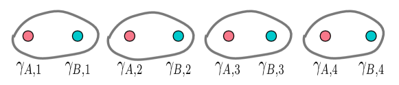
Figure 27: Here, the bonds are between Majorana modes at the same site. The ground state is unique and the end Majorana modes do not play any special role.

We first analyse the second case. Here, the fermion at each site is simply broken up into two Majorana fermions and the $\mu$ term simply couples them as shown in Fig.27. In this case, there is a unique ground state corresponding to the vacuum state with no fermions. Adding a fermion to the system costs an energy $\mu$, so the system is gapped.

Figure 28: Here, the bonds are between Majorana modes on adjacent sites. There are unpaired Majorana modes at the two ends. The ground state is doubly degenerate depending on whether the fermion state formed from the unpaired Majorana modes is occupied or unoccupied.

The first limit, on the other hand, couples Majorana modes at adjacent sites. In terms of new fermions $d_{x}=(\gamma_{B,x}+i\gamma_{A,x+1})/2$, the Hamiltonian can be rewritten as

$$H=2t\sum_{x=1}^{N-1}d_{x}^{\dagger}d_{x}$$ (76)

This clearly shows that the system has a gap and the cost of adding a fermion to the system is $2t$. But the interesting point to note is that the Hamiltonian is completely independent of the two Majorana modes $\gamma_{A,1}$ and $\gamma_{B,N}$ as shown in Fig.28, at the two ends of the wire. These two Majorana modes can be combined to form a fermion as

$$c_{M}=\frac{1}{2}(\gamma_{A,1}+i\gamma_{B,N})~{}.$$ (77)

But this is a highly non-local fermion, since $\gamma_{A,1}$ and $\gamma_{B,N}$ are localised at opposite ends of the chain. Moreover, since this fermion is absent from the Hamiltonian, the energy is the same whether or not this fermion state is occupied. So the ground state is degenerate. If $|0>$ is the ground state, then $c_{M}^{\dagger}|0>$ is also a ground state. Note that $\gamma_{a}^{2}=1$ implies that there is no Pauli principle for the Majorana modes - in fact, as we saw earlier, there is no notion of occupation number for a single Majorana mode. Number operators only exist for fermions formed from pairs of Majorana modes. Depending on the occupation or not of the zero energy mode of the fermion - i.e, of $c_{M}$ - there exists an odd or even number of fermions in the ground state referred to as ‘fermion parity’. To change the parity, electrons have to be added or removed from the superconductor. This is unlike normal gapped superconductors, (e.g. the second limit), which have a unique ground state with even fermion parity.

In the more general caseleinjse , when $\mu,t$ and $\Delta$ are non-zero, the general features of the topologically trivial case with a unique ground state, and the topologically non-trivial case with the Majorana edge states persist. Why do we call them topologically trivial and non trivial in the two cases? Well, in the trivial case there are no edge states and in the non-trivial case, there are edge states. In terms of the bulk properties of the Kitaev chain, one can find the bulk quasiparticle spectrum by going to momentum space and rewriting the Hamiltonian in Eq.69 as

$$H=\sum_{k}\zeta_{k}c_{k}^{\dagger}c_{k}+\sum_{k}(\Delta_{k}c_{k}c_{-k}+h.c.)$$ (78)

using $c_{x}=\frac{1}{\sqrt{N}}\sum_{k}e^{ikx}c_{k}$ and $c_{x}=c_{x+N}$, $\zeta_{k}=-2t\cos k-\mu$ and $\Delta_{k}=-2i\Delta\sin k$ We then find the quasi-particle spectrum by going to Nambu space and writing the Boguliobov-de Gennes Hamiltonian as

$$H=(c_{k}^{\dagger}c_{-k})\begin{pmatrix}\zeta_{k}&\Delta_{k}^{*}\\ \Delta_{k}&-\zeta_{k}\end{pmatrix}\begin{pmatrix}c_{k}^{\dagger}\\ c_{-k}\end{pmatrix}$$ (79)

and finally we get the spectrum $E_{k}=\sqrt{(\zeta_{k}^{2}+|\Delta_{k}|^{2})}$. Hence, the model is gapped, except when $\mu=-2t$ when $k=k_{F}=0$ or when $\mu=+2t$ when $k=k_{F}=\pm\pi$. The lines $\mu=\pm 2t$ are where the system becomes gapless. For $\mu<2t$, the system is topological and is adiabatically connected to the first limit with Majorana edge states. For $\mu>2t$, the system is topologically trivial and is adiabatically connected to the second limit with no edge states.

IV.2 Statistics of the Majorana modes

Figure 29: Here, we exchange the Majorana modes belonging to the same fermion. This only gives rise to a phase and hence abelian statistics.

Now, let us consider the statisticsivanov ; berg of the Majorana modes. Let us start with the simplest case where $N=1$. In this case, there are only two Majorana modes and the braid group only has a single generator $\tau$. As we saw in the first section, $\tau$ is the operator that exchanges the Majorana modes $A$ and $B$ (as shown in Fig.29) -

$$\gamma_{A}\rightarrow\gamma_{A}^{\prime}=\tau^{\dagger}\gamma_{A}\tau=e^{i\phi}\gamma_{B}~{},$$ (80)

but it does not fix the phase $\phi$ which is arbitrary. We can choose it to be +1. But then the phase of

$$\gamma_{B}\rightarrow\gamma_{B}^{\prime}=\tau^{\dagger}\gamma_{B}\tau=e^{i\phi}\gamma_{A}$$ (81)

is forced to be $-1$. This is because when there are only 2 Majorana modes, and the system is isolated, the fermion parity is forced to be conserved. The fermion state formed from the two Majorana modes is either occupied or unoccupied and we can check that

$$i\gamma_{A}\gamma_{B}=(1-2c_{M}^{\dagger}c_{M}).$$ (82)

So if the right hand side remains unchanged, then $i\gamma_{A}\gamma_{B}$ has to remain unchanged, which is only possible, if we choose the phases as shown above, since $\gamma_{A}\gamma_{B}=-\gamma_{B}\gamma_{A}$. Here, we can choose the exchange operator to be of the form

$$\tau=\frac{1}{\sqrt{2}}(1+\gamma_{A}\gamma_{B}).$$ (83)

It is easy to check that $\tau$ defined this way is unitary and that it actually carries out the exchange by substituting for $\tau$ in Eq.81. It is also easy to check that $\tau$ can be rewritten as ${\rm exp}(\pi\gamma_{A}\gamma_{B}/4)$. If we write it in terms of the fermion number operator,

$$\tau=e^{i\pi(1-2n)/4},\quad{\rm where}\quad n=c_{M}^{\dagger}c_{M}.$$ (84)

Clearly, since $n$ does not change, the statistics parameter is abelian and it cannot rotate states in the ground state manifold ($|0>,c_{M}^{\dagger}|0>$).

Now, let us see what happens when $N=2$. Here, we have 4 Majorana modes $\gamma_{i},i=A\dots D$ which can form 2 normal fermions -

$$c_{1}=\frac{1}{2}(\gamma_{A}+i\gamma_{B}),~{}~{}c_{1}^{\dagger}=\frac{1}{2}(\gamma_{A}-i\gamma_{B})$$

$$c_{2}=\frac{1}{2}(\gamma_{C}+i\gamma_{D}),~{}~{}c_{2}^{\dagger}=\frac{1}{2}(\gamma_{C}-i\gamma_{D})$$ (85)

The degenerate states of the system are given by $|n_{1},n_{2}>=c_{1}^{\dagger}c_{2}^{\dagger}|0,0>=\{|0,0>,|1,0>,|0,1>,|1,1>\}$. Operator $\tau_{AB}$ exchanges the Majoranas $A$ and $B$ keeping $C,D$ unchanged and operator $\tau_{CD}$ exchanges the Majoranas $C$ and $D$ keeping $A,B$ unchanged. Similarly, we can define, $\tau_{AC}$, $\tau_{BD}$, etc.

Figure 30: Here, we exchange the Majorana modes belonging to two different fermions. This leads to a unitary rotation in the space of degenerate states and hence, to non-abelian statistics.

It is now clear that analogous to the $N=1$ case, if we exchange the two Majorana zero modes from the same fermion, as shown in Fig.29, we will only get a phase - i.e.,

$$\tau_{AB}|n_{1},n_{2}> = e^{{i\pi(1-2n_{1})/4}}|n_{1},n_{2}>$$

$$\tau_{CD}|n_{1},n_{2}> = e^{{i\pi(1-2n_{2})/4}}|n_{1},n_{2}>~{}.$$ (86)

In the first equation, $n_{2}$ comes along for a ride and in the second equation, $n_{1}$ comes along for a ride. So both these operators are abelian operators. But now, let us exchange one Majorana from one of the fermions with another Majorana from the other fermion, (as shown in Fig.30) -

$$\tau_{BC}=\frac{1}{\sqrt{2}}(1+\gamma_{B}\gamma_{C}).$$ (87)

In terms of the fermions $c_{1}$ and $c_{2}$, this can be written as

$$\tau_{BC}=\frac{1}{\sqrt{2}}[1-i(c_{1}-c_{1}^{\dagger})(c_{2}+c_{2}^{\dagger})].$$ (88)

Now acting this on $|n_{1},n_{2}>$ does not lead to a phase. Instead, it leads to a rotation in the space of degenerate states given by

$$\tau_{BC}|n_{1},n_{2}>=\frac{1}{\sqrt{2}}[|n_{1},n_{2}>+i(-1)^{n_{1}}|1-n_{1},1-n_{2}>]~{}.$$ (89)

If we now consider sequential exchanges, it is clear that different exchanges will not commute with one another - the final state will depend on the order of the operations. This is what is meant by saying that the Majorana particles have non-abelian statistics under exchange.

The derivation of the non-abelian statistics is not dependent on the details of how the exchange between the particles is carried out, and hence it cannot be changed by disorder or local details. It is topologically stable.

To understand multiple non-abelian anyons, as we already mentioned, we need to understand fusion paths, since the fusion rules do not need to unique results. These fusion paths represent a basis of the degenerate ground state manifold, and are most conveniently studied in terms of conformal blocks of the appropriate conformal field theoryanyonsqc . But that is beyond the scope of these lectures and we will stop here.

V Conclusion

Let me conclude by repeating the main message of these lectures - understanding the notion of anyons and non-abelian anyons is an exciting field today. The study of these excitations could lead to an understanding of concepts like decoherence and entanglement which are relevant in quantum computation. Work on non-abelian states, in general, is still in its infancy. For young researchers, hence, this should be a useful and relevant topic of study at the crossroads of condensed matter physics and quantum information. For more information and references, there are many recent reviewsstern ; anyonsqc ; alicea available on the net.

References

- (1) J. M. Leinaas and J. Myrrheim, Il Nuovo Cimento, 37, 1 (1977).
- (2) See for instance, review by A. Stern, ‘Anyons and the quantum Hall effect - a pedagogical review’, cond-mat/0711.4697.
- (3) C. Nayak, S. H. Simon, M. Freedman and S. D. Sarma, Rev. Mod. Phys. 80 1083 (2008).
- (4) See review by S. Rao, ‘An Anyon Primer’, hep-th/9209066 based on Lectures delivered at the VIII SERC School in High Energy Physics, 30 Dec. ’91 - 18 Jan ’92, held at Physical Research Laboratory, Ahmedabad, and at the I SERC School in Statistical Mechanics, Feb ’94, held at Puri, published in ’Models and Techniques of Statistical Physics’, edited by S. M. Bhattacharjee (Narosa Publications).
- (5) ‘Anyons’ Alberto Lerda, Lecture notes in Physics Monographs, Series 14, Springer-Verlag publications, 1992.
- (6) ‘Fractional statistics and quantum theory’, A. Khare, World Scientific, 1998.
- (7) See for instance, ‘Fractional statistics and Anyon Superconductivity’, edited by F. Wilczek, Series on directions in condensed matter physics, World Scientific Publications, October 1990.
- (8) F. Wilczek, Phys. Rev. Lett. 48, 1144 (1982); ibid, 49, 957 (1982).
- (9) A. Kitaev, ‘Fault tolerant quantum computation by anyons’, Ann. Phys. 321, 2 (2003).
- (10) A. Kitaev and C. Laumann, ‘Topological phases and quantum computation’, 0904.2771, lectures given by A. Kitaev at the 2008 Les Houches summer school ‘Exact methods in low-dimensional physics and quantum computing’.
- (11) M. Burello, ‘Topological order and quantum computation: Toric code’ , talk available on the net.
- (12) A. Y. Kitaev, ‘Unpaired Majorana fermions in quantum wires’, Physics-Uspekhi, 44, 131 (2001).
- (13) G. Moore and N. Read, Nucl. Phys. B360, 362 (1991).
- (14) R. S. K. Mong et al, Phys. Rev. X4, 011036 (2014).
- (15) J. Alicea, ‘New directions in the pursuit of Majorana fermions in solid state systems’, cond-mat/1202.1293, Rep. Prog. Phys. 75, 076501 (2012).
- (16) X. G. Wen, Int. J. Mod. Phys. B4, 239 (1990); X. G. Wen and Q. Niu, Phys. Rev. BB 41, 9377 (1990).
- (17) J. Preskill, ‘Lecture notes for Physics 219: Quantum computation’ http://www.theory.caltech.edu/ preskill/ph219/topological.pdf
- (18) M. Leinjse and K. Flensberg, cond-mat/1206.1736, Semicond. Sci. Technol. 27, 124003 (2012).
- (19) D. A. Ivanov, Phys. Rev. Lett. 86, 268 (2001).
- (20) E. Berg, ‘Anyonic statistics : A new paradigm for non-abelian statistics’, talk available on the net.