Shortcut to adiabatic population transfer in quantum three-level systems: effective two-level problems and feasible counter-diabatic driving

Abstract

Shortcut to adiabaticity in various quantum systems has attracted much attention with the wide applications in quantum information processing and quantum control. In this paper, we concentrate on stimulated Raman shortcut-to-adiabatic passage in quantum three-level systems. To implement counter-diabatic driving but without additional coupling, we first reduce the quantum three-level systems to effective two-level problems at large intermediate-level detuning, or on resonance, apply counter-diabatic driving along with the unitary transformation, and eventually modify the pump and Stokes pulses for achieving fast and high-fidelity population transfer. The required laser intensity and stability against parameter variation are further discussed, to demonstrate the advantage of shortcuts to adiabaticity.

I INTRODUCTION

Coherent manipulation of internal state in various quantum systems plays a significant role in atomic and molecular physics with the applications in metrology, interferometry, quantum computing, quantum information processing and control of chemical interaction, see review Bergmann-Rev ; Guerin ; Shapiro-Rev ; Molmer ; Bergmann-Rev2 . Quite often, one of the most important goals is to achieve state preparation or transfer with high fidelity. So adiabatic approaches such as rapid adiabatic passage (RAP), stimulated Raman adiabatic passage (STIRAP) and their variants Shapiro-Rev ; Molmer ; Bergmann-Rev2 have been proposed and widely applied in different quantum two-level or three-level systems. These adiabatic protocols are robust against the fluctuations of control parameters, as compared to the resonant pulses. However, the long time required to satisfy the adiabatic criteria might be problematic, when the decoherence effect is considered. Therefore, in order to achieve fast and high-fidelity quantum state control, the optimal control theory Tannor ; Boscain ; Kontz ; Vitanov-opt and composite pulses Levitt ; Torosov-PRL ; Torosov have been proposed, by reducing the time consumption and diabatic loss or minimizing systematic errors.

Alternatively, several works on “shortcut to adiabaticity” (STA), including counter-diabatic, inverse engineering, and fast-forward approaches, have been recently devoted to mimicking adiabatic population transfers but within a short time Berry ; Rice ; PRL105 ; ChenPRA11 ; Ruschhaupt ; GuerinPRL ; ChenPRA12 ; Arimondo ; Longhi-nonHermite ; Sofia ; Masuda ; SongXK ; Xiayan ; Clerk . Among them, the counter-diabatic driving Rice (equivalent to transitionless quantum algorithm Berry ) provides a powerful method to design complementary interaction appropriately, so that diabatic transition can be suppressed and the system evolves exactly following the adiabatic reference. Such shortcut protocol has been experimentally demonstrated in (effective) two-level quantum systems, e.g. accelerated optical lattice Oliver and spin of a single NV center in diamond Suter . In the three-level atomic systems, additional coupling between initial and target levels can be implemented by a magnetic dipole transition PRL105 ; Unanyan , which might be problematic in practice. In other systems, it might be even unfeasible. The way out is to apply the unitary transformation for cancelling the additional coupling but keeping the same dynamics PRL109 ; Takahashi ; SongXK , or the (generalized) inverse engineer for pulse shapes ChenPRA12 ; Clerk . However, in many cases the examples of three-level system on one-photon resonance have been worked out for simplicity.

Figure 1: $\Lambda$-type three-level system for STIRAP, where the Rabi frequencies $\Omega_{p,s}$ present the pump and Stokes pulses, $\Delta$ and $\Delta_{s}$ are the detunings.

In this paper, we shall concentrate on the construction and implementation of stimulated Raman shortcut-to-adiabatic passage (STIRSAP) in quantum three-level systems, see Fig. 1. Particularly, large intermediate-level detuning or one-photon resonance are assumed here, since STIRAP in these cases can be reduced to effective two-level problems VitanovPRA . This allows us to utilize the counter-diabatic technique along with unitary transformation proposed in two-level systems PRL109 , thus implementing STIRSAP without additional coupling by only modifying pump and Stokes pulses. In detail, in the case of large detuning, we first reduce the quantum three-level system to an effective two-level system by using “adiabatic elimination”, apply counter-diabatic driving along with the unitary transformation, and finally design pump and Stokes pulses. For the sake of completeness, the counter-diabatic driving in one-photon resonance case and the connection with other shortcut methods is studied. At last, the stability with respect to the parameter fluctuation is also discussed, showing the advantage of STA. STIRSAP proposed here can be demonstrated in recent experiments for speeding up SITRAP with cold atom NC and solid-state spin systems NV-3level .

II MODEL and HAMILTONIAN

Considering the Hamiltonian for STIRAP system within the rotating wave approximation (RWA) Bergmann-Rev ; Bergmann-Rev2 ; ChenPRA12

$$H_{0}=\frac{\hbar}{2}\left(\begin{array}[]{ccc}0&\Omega_{p}(t)&0\\ \Omega_{p}(t)&2\Delta&\Omega_{s}(t)\\ 0&\Omega_{s}(t)&2\delta_{s}\end{array}\right).$$ (1)

Here $\Omega_{p}(t)$ and $\Omega_{s}(t)$ are Rabi frequencies of pump and Stokes laser fields, shown in Fig. 1, where $\Delta=(E_{2}-E_{1})/\hbar-\omega_{p}$, $\Delta_{s}=(E_{2}-E_{3})/\hbar-\omega_{s}$, and $\delta_{s}=\Delta-\Delta_{s}$, $\omega_{p}$ and $\omega_{s}$ are the laser frequencies of pump and Stokes laser, respectively, and $E_{j},j=1,2,3$ are bare-basis state energies. On two-photon resonance ($\delta_{s}=0$), the Hamiltonian (1) reads

$$H_{0}=\frac{\hbar}{2}\left(\begin{array}[]{ccc}0&\Omega_{p}(t)&0\\ \Omega_{p}(t)&2\Delta&\Omega_{s}(t)\\ 0&\Omega_{s}(t)&0\end{array}\right),$$ (5)

whose instantaneous eigenstates are

$$|n_{0}\rangle=\cos\theta|1\rangle-\sin\theta|3\rangle,~{}~{}$$

$$|n_{+}\rangle=\sin\theta\sin\varphi|1\rangle+\cos\varphi|2\rangle+\cos\theta\sin\varphi|3\rangle,$$

$$|n_{-}\rangle=\sin\theta\cos\varphi|1\rangle-\sin\varphi|2\rangle+\cos\theta\cos\varphi|3\rangle,$$

with eigenvalues $E_{+}(t)=\hbar\Omega\cot(\varphi/2)$, $E_{0}=0$, and $E_{-}(t)=-\hbar\Omega\tan(\varphi/2)$. Two mixing angles are defined by $\tan\theta=\Omega_{p}(t)/\Omega_{s}(t)$ and $\tan(2\varphi)=\Omega/\Delta(t)$, with $\Omega=[\Omega^{2}_{p}(t)+\Omega^{2}_{s}(t)]^{1/2}$. The wave functions of this three-level system, $\textbf{c}(t)=[c_{1}(t),c_{2}(t),c_{3}(t)]^{T}$, denoted by $|1\rangle$, $|2\rangle$ and $|3\rangle$, is governed by the time-dependent Schrödinger equation $i\hbar d\textbf{c}(t)/dt=H_{0}\textbf{c}(t)$. Once these conditions for adiabatic following, $\dot{\theta}\ll\Omega$ (local) and $\Omega t_{f}\gg 1$ (global), are satisfied Bergmann-Rev ; Bergmann-Rev2 , the solution of above Schrödinger equation coincides with the adiabatic approximation, thus the population can be transferred $|1\rangle$ to $|3\rangle$ along the “dark state” $|n_{0}\rangle$, where $t_{f}$ is the pulse duration or the so-called operation time.

In order to reproduce STIRAP but within a short time, that is, achieve fast population transfer from $|1\rangle\rightarrow|3\rangle$, one can apply the counter-diabatic driving Rice (equivalent to quantum transitionless algorithm Berry ; PRL105 ),

$$H_{cd}=i\hbar\sum|\partial_{t}n{\rangle}{\langle}n|,$$ (6)

to design the supplementary interaction in the form of PRL105

$$H_{cd}=\frac{\hbar}{2}\begin{pmatrix}0&0&i\Omega_{a}(t)\\ 0&0&0\\ -i\Omega_{a}(t)&0&0\end{pmatrix},$$ (7)

with $\Omega_{a}(t)=2[\dot{\Omega}_{p}(t)\Omega_{s}(t)-\dot{\Omega}_{s}(t)\Omega_{p}(t)]/[\Omega_{p}^{2}(t)+\Omega_{s}^{2}(t)]$. The additional coupling between $|1{\rangle}$ and $|3{\rangle}$, implemented by microwave dipole transition in atomic system Unanyan , can completely suppress the diabatic transition. However, such coupling might be difficult or even impossible to implement in various systems. For instance, the phase mismatch between laser and microwave fields causes the infidelity NC . Moreover, generating the grating for such coupling is doable in optical multi-mode waveguide, but not in coupled waveguides ShuoOE . In general, when $\Delta\neq 0$ under the two-photon resonance condition, the cancellation of counter-diabatic interaction becomes more challenging by using unitary transformation, as compared to the case of one-photon resonance ($\Delta=0$), since the eight Gell-Mann matrices are involved in the dynamics of such three-level systems satisfying SU(3) Lie algebra Hioe . In what follows we shall propose the method of implementation of counter-diabatic driving in three-level systems. Following VitanovPRA , we reduce STIRAP to the effective two-level problems by considering the adiabatic elimination under large detuning ($\Delta\gg\Omega$) or one-photon resonance ($\Delta=0$), which enables to implement STIRSAP without additional coupling by using the similar strategy originally proposed in two-level systems PRL109 .

As we shall deal with two different examples with the assumption of large detuning and one-photon resonance. It is unavoidable to repeat some symbols, such as $H_{cd}$, $\Omega_{a}(t)$, $\theta$, $H_{\textrm{eff}}$, $\tilde{H}_{\textrm{eff}}$, $\Omega_{\textrm{eff}}(t)$, $\Delta_{\textrm{eff}}(t)$, $\tilde{\Omega}_{\textrm{eff}}(t)$, $\tilde{\Delta}_{\textrm{eff}}(t)$, and $\tilde{\Omega}_{p,s}(t)$. So consistency is strictly guaranteed only within each case. The detail of how this comes about will be clarified in the context.

III Feasible shortcut design

III.1 large detuning ($\Delta\gg\Omega$)

At large intermediate-level detuning, $\Delta\gg\Omega$, level $|2\rangle$ is scarcely populated ($\dot{c}_{2}(t)\simeq 0$), and it can be adiabatically eliminated to obtain the following effective two-level Hamiltonian in the subspace of levels $|1\rangle$ and $|3\rangle$ VitanovPRA :

$$H_{\textrm{eff}}=\frac{\hbar}{2}\begin{pmatrix}-\Delta_{\textrm{eff}}(t)&\Omega_{\textrm{eff}}(t)\\ \Omega_{\textrm{eff}}(t)&\Delta_{\textrm{eff}}(t)\end{pmatrix},$$ (8)

where the effective detuning $\Delta_{\textrm{eff}}(t)$ and Rabi frequency $\Omega_{\textrm{eff}}(t)$ are

$$\Delta_{\textrm{eff}}(t)=\frac{\Omega_{p}^{2}(t)-\Omega_{s}^{2}(t)}{4\Delta},$$ (9)

$$\Omega_{\textrm{eff}}(t)=-\frac{\Omega_{p}(t)\Omega_{s}(t)}{2\Delta}.$$ (10)

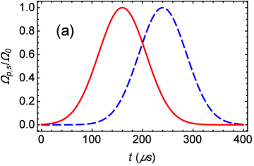
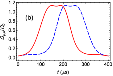
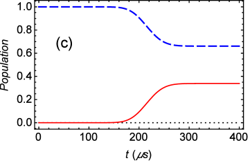
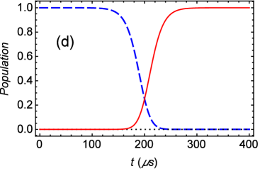
Figure 2: (Color online) Different Rabi frequencies for STIRAP (a) and STIRSAP (b), where Stokes (solid red) and pump (dashed blue) pulses are shown. The state evolutions of STIRAP (c) and STIRSAP (d) are also compared, where population of levels $|1\rangle$ (dashed blue), $|2\rangle$ (dotted black), and $|3\rangle$ (solid red) is presented. Parameters: $\Omega_{0}=2\pi\times 5$ MHz, $\Delta=2\pi\times 2.5$ GHz, $t_{f}=400$ $\mu$s, $\tau=t_{f}/10$ and $\sigma=t_{f}/6$.

Once the effective two-level Hamiltonian (8) is obtained, we can calculate the counter-diabatic driving, from the definition (6), as PRL105

$$H_{cd}=\frac{\hbar}{2}\begin{pmatrix}0&-i\Omega_{a}(t)\\ i\Omega_{a}(t)&0\end{pmatrix},$$ (11)

where $\Omega_{a}(t)=[\Omega_{\textrm{eff}}(t)\dot{\Delta}_{\textrm{eff}}(t)-\dot{\Omega}_{\textrm{eff}}(t)\Delta_{\textrm{eff}}(t)]/[\Delta_{\textrm{eff}}^{2}(t)+\Omega_{\textrm{eff}}^{2}(t)]$. Assisted by the counter-diabatic term (11), the system can be driven along the adiabatic path of reference Hamiltonian (8) within a short time. The total Hamiltonian, $H=H_{\textrm{eff}}+H_{cd}$, is constructed as

$$H=\frac{\hbar}{2}\begin{pmatrix}-\Delta_{\textrm{eff}}(t)&\sqrt{\Omega_{\textrm{eff}}^{2}(t)+\Omega_{a}^{2}(t)}e^{-i\phi}\\ \sqrt{\Omega_{\textrm{eff}}^{2}(t)+\Omega_{a}^{2}(t)}e^{i\phi}&\Delta_{\textrm{eff}}(t)\end{pmatrix},$$ (12)

where $\phi(t)=\arctan[\Omega_{a}(t)/\Omega_{\textrm{eff}}(t)]$. By applying the unitary transformation,

$$U(t)=\begin{pmatrix}e^{-i\phi(t)/2}&0\\ 0&e^{i\phi(t)/2}\end{pmatrix},$$ (13)

we can further obtain $\tilde{H}_{\textrm{eff}}=U^{{\dagger}}HU-i\hbar U^{{\dagger}}\dot{U}$, namely,

$$\tilde{H}_{\textrm{eff}}=\frac{\hbar}{2}\begin{pmatrix}-\tilde{\Delta}_{\textrm{eff}}(t)&\tilde{\Omega}_{\textrm{eff}}(t)\\ \tilde{\Omega}_{\textrm{eff}}(t)&\tilde{\Delta}_{\textrm{eff}}(t)\end{pmatrix},$$ (14)

with $\tilde{\Delta}_{\textrm{eff}}(t)=\Delta_{\textrm{eff}}(t)+\dot{\phi}$ and $\tilde{\Omega}_{\textrm{eff}}(t)=\sqrt{\Omega_{\textrm{eff}}^{2}(t)+\Omega_{a}^{2}(t)}$. Obviously, the unitary transformation means the rotation along $z$-axis, which results in the cancellation of $\sigma_{y}$ term in the Hamiltonian (12). In principle, the population dynamics of Hamiltonian (14) is the same as the previous one (12), up to the global phase. When the boundary condition $U(0)=U(t_{f})=1$ is satisfied, the initial and final population is the same as the adiabatic reference. Now let us go back to the three-level system and design the modified pump and Stokes fields by comparing the Hamiltonian (14) and (8). Like Eqs. (9) and (10), we impose

$$\tilde{\Delta}_{\textrm{eff}}(t) = \frac{\tilde{\Omega}_{p}^{2}-\tilde{\Omega}_{s}^{2}}{4\widetilde{\Delta}},$$ (15)

$$\tilde{\Omega}_{\textrm{eff}}(t) = -\frac{\tilde{\Omega}_{p}(t)\tilde{\Omega}_{s}(t)}{2\widetilde{\Delta}},$$ (16)

and calculate inversely the modified fields as

$$\tilde{\Omega}_{p}(t) = \sqrt{2\widetilde{\Delta}(\sqrt{\tilde{\Delta}^{2}_{\textrm{eff}}(t)+\tilde{\Omega}^{2}_{\textrm{eff}}(t)}+\tilde{\Delta}_{\textrm{eff}}(t))},$$ (17)

$$\tilde{\Omega}_{s}(t) = \sqrt{2\widetilde{\Delta}(\sqrt{\tilde{\Delta}^{2}_{\textrm{eff}}(t)+\tilde{\Omega}^{2}_{\textrm{eff}}(t)}-\tilde{\Delta}_{\textrm{eff}}(t))}.$$ (18)

In order to guarantee that the problem of a two-level system with counter-diabatic term can be transformed back to a three-level system with modified Stokes and pumping pulses, we should have $\widetilde{\Delta}\gg\tilde{\Omega}_{p,s}(t)$. Here it is reasonable to assume $\widetilde{\Delta}=\Delta$, since the original detuning $\Delta$ is the order of GHz, but the (modified) Rabi frequency is the order of MHz, see the parameters in Fig. 2. Substituting the expressions of $\tilde{\Omega}_{\textrm{eff}}(t)$ and $\tilde{\Delta}_{\textrm{eff}}(t)$ into Eqs. (17) and (18), we finally obtain new designed laser fields to drive the state following the dynamics of effective two-level Hamiltonian (14), thus implementing STIRSAP at large intermediate-level detuning.

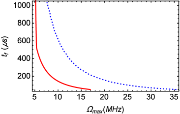
Figure 3: (Color online) Operation time $t_{f}$ versus the peak value of Rabi frequency $\Omega_{\textrm{max}}$ for STIRSAP (solid red) and STIRAP (dashed blue) when the fidelity is above $99\%$. Parameters are the same as those in Fig. 2.

To illustrate how shortcut protocol works for STIRAP, we assume the original pump and Stokes pulses, see Fig. 2 (a), as an adiabatic reference,

$$\Omega_{p}(t)=\Omega_{0}\,\exp\,\left[-\frac{(t-t_{f}/2-\tau)^{2}}{\sigma^{2}}\right],$$ (19)

$$\Omega_{s}(t)=\Omega_{0}\,\exp\,\left[-\frac{(t-t_{f}/2+\tau)^{2}}{\sigma^{2}}\right],$$ (20)

with full width at half maximum (FWHM) $\sigma$, separation time between the two pulses $\tau$, and the amplitude $\Omega_{0}$. We set the detuning $\Delta=2\pi\times 2.5$ GHz to guarantee large detuning, $\Delta\gg\Omega_{0}$, for the validity of “adiabatic elimination”. In this case, the operation time required for adiabatic process should be larger than resonant $\pi$ pulse, $t_{f}\gg t_{\pi}=2\pi\Delta/\Omega^{2}_{0}$. Under the parameters: $\Omega_{0}=2\pi\times 5$ MHz, $t_{f}=400$ $\mu$s ($t_{\pi}=100$ $\mu$s), $\tau=t_{f}/10$ and $\sigma=t_{f}/6$, the dynamics of original Hamiltonian (5) with pump and Stokes pulses, see Eqs. (19) and (20), is not adiabatic at all, and population is not completely transferred from $|1\rangle$ to $|3\rangle$, see Fig. 2 (c). By using modified pulses predicted from Eqs. (17) and (18), the perfect population transfer can be achieved within a short time, as shown in Figs. 2 (b) and (d). The shapes of modified pump and Stokes pulse are smooth enough to generate in the experiment with cold atoms NC , though they are slightly different from original Gaussian ones.

Importantly, we have to point out the energy cost for the acceleration of STIRAP. By comparing the pulses in STIRAP and STIRSAP, we see that the peak value of modified Rabi frequencies is larger than original ones. It is reasonable that more laser intensity is required to shorten the operation time, and the relation between energy (laser intensity) and operation time, in general, satisfies $\Omega_{\textrm{max}}\propto 1/t_{f}$. To quantify it, we plot the operation time versus maximum value of laser intensity $\Omega_{\textrm{max}}$ in Fig. 3. Given the fidelity above $99.99\%$, the maximum laser intensity required for shortcuts is less than that for STIRAP. In other words, when an allowed laser intensity is fixed, the operation time for STIRSAP is less than that for conventional STIRAP. For example, if the maximum value of laser intensity is $\Omega_{\textrm{max}}=2\pi\times 10$ MHz, the time required for STIRSAP is $t_{f}=145$ $\mu$s, which is about 4.3 times faster than the original STIRAP, $t_{f}=620$ $\mu$s.

III.2 one-photon resonance ($\Delta\equiv 0$)

On one-photon resonance, $\Delta=0$, the three-level system is similarly reduced to the following effective two-level system VitanovPRA ,

$$H_{\textrm{eff}}=\frac{\hbar}{2}\begin{pmatrix}-\Delta_{\textrm{eff}}(t)&\Omega_{\textrm{eff}}(t)\\ \Omega_{\textrm{eff}}(t)&\Delta_{\textrm{eff}}(t)\end{pmatrix},$$ (21)

with effective Rabi frequency and detuing, $\Omega_{\textrm{eff}}(t)=\Omega_{p}(t)/2$ and $\Delta_{\textrm{eff}}(t)=-\Omega_{s}(t)/2$. Noting that the Hamiltonian (5) on resonance ($\Delta=0$) has the same form as the optical Bloch equations for such effective two-level system (in units $\hbar=1$) Carroll ; Laine . The probability amplitudes $c_{j}(t)$ of the three-level system with Hamiltonian (5) are related to the corresponding two-level amplitudes $b_{j}(t)$ by $c_{1}(t)=|b_{1}(t)|^{2}-|b_{2}(t)|^{2}$, $c_{2}(t)=2i\mbox{Im}[b_{1}^{*}(t)b_{2}(t)]$, and $c_{3}(t)=-2\mbox{Re}[b_{1}^{*}(t)b_{2}(t)]$, where $j$ denotes the number of states. Again, the total Hamiltonian is $H=H_{\textrm{eff}}+H_{cd}$, where the counter-diabatic term is calculated as PRL105

$$H_{cd}=\frac{\hbar}{2}\begin{pmatrix}0&-i\Omega_{a}(t)\\ i\Omega_{a}(t)&0\end{pmatrix}.$$ (22)

with $\Omega_{a}(t)=[\dot{\Omega}_{p}(t)\Omega_{s}(t)-\dot{\Omega}_{s}(t)\Omega_{p}(t)]/[\Omega_{p}^{2}(t)+\Omega_{s}^{2}(t)]$. After $z$-axis rotation by using unitary transformation (13), we can obtain

$$\tilde{H}_{\textrm{eff}}=\frac{\hbar}{2}\begin{pmatrix}-\tilde{\Delta}_{\textrm{eff}}(t)&\tilde{\Omega}_{\textrm{eff}}(t)\\ \tilde{\Omega}_{\textrm{eff}}(t)&\tilde{\Delta}_{\textrm{eff}}(t)\end{pmatrix},$$ (23)

with the new definition, $\tilde{\Delta}_{\textrm{eff}}(t)=\Delta_{\textrm{eff}}(t)+\dot{\phi}$, $\tilde{\Omega}_{\textrm{eff}}(t)=[\Omega_{\textrm{eff}}^{2}(t)+\Omega_{a}^{2}(t)]^{1/2}$, and $\phi(t)=\arctan[2\Omega_{a}(t)/\Omega_{p}(t)]$. Supposing the two-level problem can be transformed back to three-level problem, we can impose $\tilde{\Omega}_{\textrm{eff}}(t)=\tilde{\Omega}_{p}(t)/2$ and $\tilde{\Delta}_{\textrm{eff}}(t)=-\tilde{\Omega}_{s}(t)/2$, and the modified pump and Stokes Rabi frequency can be inversely calculated as

$$\tilde{\Omega}_{p}(t) = \sqrt{\Omega_{p}^{2}(t)+4\Omega_{a}^{2}(t)},$$ (24)

$$\tilde{\Omega}_{s}(t) = \Omega_{s}(t)-2\dot{\phi}(t).$$ (25)

Figs. 4 (a) and (b) show the new designed pump and Stokes pulses, as compared to the original ones. The evolution of state in Figs. 4 (c) and (d) demonstrates that by using STIRSAP the population transfer can be achieved with fidelity $1$, while the previous STIRAP does not work perfectly. The parameters are $\Omega_{0}=2\pi\times 5$ MHz, $t_{f}=1$ $\mu$s, $\tau=t_{f}/8$ and $\sigma=t_{f}/6$. The operation time used here is very short, and not much larger than $t_{\pi}=\sqrt{2}\pi/\Omega_{0}\simeq 0.14$ $\mu$s for resonant $\pi$ pulse. So the influence of spontaneous emission might be negligible, though the level $|2\rangle$ is populated.

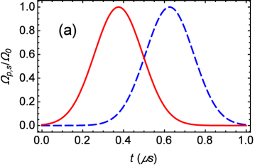
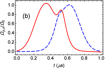
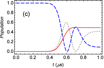
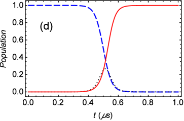
Figure 4: (Color online) Different Rabi frequencies for STIRAP (a) and STIRSAP (b), where Stokes (solid red) and pump (dashed blue) pulses are shown. The state evolutions of STIRAP (c) and STIRSAP (d) are also compared, where population of levels $|1\rangle$ (dashed blue), $|2\rangle$ (dotted black), and $|3\rangle$ (solid red) is presented. Parameters: $\Omega_{0}=2\pi\times 5$ MHz, $t_{f}=1$ $\mu$s, $\tau=t_{f}/8$ and $\sigma=t_{f}/6$.

Fig. 5 shows that the final population transfer is sensitive to the variation of separation time $\tau$, described by $(1+\delta)\tau$. When decreasing $\tau$, the fidelity becomes worse. However, in the case of large detuning, the fidelity is robust against the fluctuation of severation time $\tau$ NC . As a matter of fact, it is relevant to the mapping between two and three-level problems. When the total Hamiltonian $H=H_{\textrm{eff}}+H_{cd}$ for the effective two-level system is transformed back to the three-level problem, the Hamiltonian will have the direct coupling $\Omega_{a}(t)$ between level $|1\rangle$ and $|3\rangle$. But after applying the unitary transformation $U$, the population dynamics of the Hamiltonian $\tilde{H}_{\textrm{eff}}$ is determined by $\widetilde{\mathbf{b}}(t)=[b^{\prime}_{1}(t)e^{i\phi/2},b^{\prime}_{2}(t)e^{-i\phi/2}]^{T}$, where $b^{\prime}_{j}(t)$ is the probability amplitudes of two-level systems with Hamiltonian $H=H_{\textrm{eff}}+H_{cd}$. When going back to three-level system, we can calculate the probability amplitudes of three-level problem from $\widetilde{c}_{1}(t)=|b^{\prime}_{1}(t)|^{2}-|b^{\prime}_{2}(t)|^{2}$, $\widetilde{c}_{2}(t)=2i\mbox{Im}[{b^{\prime}}^{*}_{1}(t)b^{\prime}_{2}(t)e^{-i\phi}]$, and $\widetilde{c}_{3}(t)=-2\mbox{Re}[{b^{\prime}}^{*}_{1}(t)b^{\prime}_{2}(t)e^{-i\phi}]$. This provides the population of level $|3\rangle$,

$$P_{3}(t)\equiv|\widetilde{c}_{3}(t)|^{2}=\cos^{2}[\phi(t)].$$ (26)

Clearly, when $\phi(t_{f})=0$, the full population transfer, $P_{3}(t_{f})=1$, can be achieved. This suggests the condition that the two-level problem can be transformed back to the three-level problem on resonant case. For example, the phase $\phi(t_{f})$ saturates to null when $\tau$ increasing, see the inset in Fig. 5, and the final population becomes irrelevant to the shift of separation time. In fact, the condition, $U(0)=U(t_{f})=1$, guarantees that the populations at initial and final time are the same before and after the unitary transformation PRL109 . So one can further choose other functions of adiabatic reference, satisfying $\phi(0)=\phi(t_{f})=0$, instead of Eqs. (19) and (20).

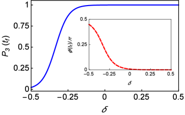
Figure 5: (Color online) Fidelity (solid blue) versus the variation of separation time $(1+\delta)\tau$. Inset: Dependence of phase $\phi$ (solid red) versus $\delta$ for further explanation. Parameters are the same of those in Fig. 4.

Furthermore, as we know, three-level system on one-photon resonance satisfies intrinsic SU(2) Lie algebra, which simplifies the shortcut design. To clarify it, we rewrite the total Hamiltonian, $H=H_{0}+H_{cd}$, on resonance, as

$$H=\frac{1}{2}[\Omega_{p}(t)\lambda_{1}+\Omega_{s}(t)\lambda_{6}-2\Omega_{a}(t)\lambda_{5}],$$ (27)

where the Gell-Mann matrices,

$$\lambda_{1}=\begin{pmatrix}0&1&0\\ 1&0&0\\ 0&0&0\end{pmatrix},\lambda_{5}=\begin{pmatrix}0&0&-i\\ 0&0&0\\ i&0&0\end{pmatrix},\lambda_{6}=\begin{pmatrix}0&0&0\\ 0&0&1\\ 0&1&0\end{pmatrix},$$

are introduced, and satisfy the commutation relation, $[\lambda_{1},\lambda_{5}]=-i\lambda_{6}$, $[\lambda_{5},\lambda_{6}]=-i\lambda_{1}$, and $[\lambda_{6},\lambda_{1}]=-i\lambda_{5}$. To get rid of the counter-diabatic term, we introduce the unitary transformation $U(t)=e^{-i\phi(t)\lambda_{6}}$, that is,

$$U(t)=\begin{pmatrix}1&0&0\\ 0&\cos\phi(t)&-i\sin\phi(t)\\ 0&-i\sin\phi(t)&\cos\phi(t)\end{pmatrix},$$ (28)

so that the Hamiltonian, $\tilde{H}=U^{{\dagger}}HU-iU^{{\dagger}}\dot{U}$, becomes

$$\tilde{H}=\frac{1}{2}[\tilde{\Omega}_{p}(t)\lambda_{1}+\tilde{\Omega}_{s}(t)\lambda_{6}-\tilde{\Omega}_{a}(t)\lambda_{5}],$$ (29)

where the Rabi frequencies are

$$\tilde{\Omega}_{p}(t) = \Omega_{p}(t)\cos\phi(t)+2\Omega_{a}(t)\sin\phi(t),$$ (30)

$$\tilde{\Omega}_{s}(t) = \Omega_{s}(t)-2\dot{\phi}(t),$$ (31)

$$\tilde{\Omega}_{a}(t) = 2\Omega_{a}(t)\cos\phi(t)-\Omega_{p}(t)\sin\phi(t).$$ (32)

Imposing $\tilde{\Omega}_{a}(t)=0$ gives $\phi(t)=\arctan[2\Omega_{a}(t)/\Omega_{p}(t)]$, which exactly results in Eqs. (24) and (25). By choosing alternative unitary transformation, $U(t)=e^{-i\phi(t)\lambda_{1}}$, we have the modified pump and Stokes pulses accordingly in the form of

$$\tilde{\Omega}_{p}(t) = \Omega_{p}(t)-2\dot{\phi}(t),$$ (33)

$$\tilde{\Omega}_{s}(t) = \sqrt{\Omega_{s}^{2}(t)+4\Omega_{a}^{2}(t)}.$$ (34)

Clearly, STIRSAP is achieved with the appropriate boundary condition $U(0)=U(t_{f})=1$. This argument is consistent with the condition that the two-level problem can be transformed back to the three-level problem on resonance. Otherwise, the population can not be exactly transferred from $|1\rangle$ to $|3\rangle$, see Fig. 5, due to the transformation. It turns out that it is not necessary to reduce the three-level system on one-photon resonance to the effective two-level problem, since the system has symmetry of SU(2). As a matter of fact, we can further choose a general unitary transformation $U(t)=\exp{\{-i[\alpha(t)\lambda_{1}+\beta(t)\lambda_{5}+\gamma(t)\lambda_{6}]\}}$, and have more flexibility to design the optimal shortcut, similar to the proposal in the literature Clerk . This suggests that shortcut methods are mathematically equivalent ChenPRA11 ; ChenPRA12 , though their physical implementation is totally different. Besides, high-order iteration can be applied, in terms of superadiabtic concept SongXK .

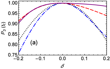
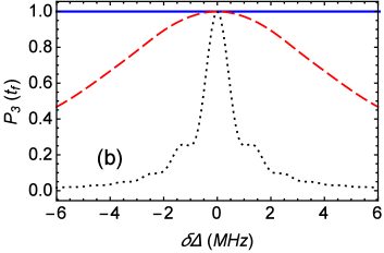
Figure 6: (Color online) (a) Population of level $|3\rangle$ at final time, $P_{3}(t_{f})$, versus the variation of laser intensity, where STIRSAP at large detuning: $t_{f}=1000$ $\mu$s (solid purple) and $t_{f}=400$ $\mu$s (dot-dashed blue); STIRSAP on one-photon resonance: $t_{f}=1$ $\mu$s (dashed red); resonant $\pi$ pulse: $t_{f}=1$ $\mu$s (dotted black). (b) $P_{3}(t_{f})$ versus the variation of detuning, where STIRSAP at large detuning: $t_{f}=400$ $\mu$s (solid blue); STIRSAP on one-photon resonance: $t_{f}=1$ $\mu$s (dashed red); resonant $\pi$ pulse: $t_{f}=1$ $\mu$s (dotted black). Other parameters are the same as those in Figs. 2 and 4.

IV DISCUSSION

In this section, we turn to discuss the stability of STIRSAP with respect to different systematic errors. Fig. 6 (a) shows that such shortcut protocol on one-photon resonance is more robust than the resonant $\pi$ pulse (with constant Rabi frequency $\Omega_{0}=\sqrt{2}\pi/t_{f}$), when the fluctuation of laser intensity is induced, described by $(1+\delta)\Omega_{s,p}$ or $(1+\delta)\tilde{\Omega}_{s,p}$. On the contrary, the shortcut protocol at large detuning is not as stable as the shortcut on one-photon resonance and resonant $\pi$ pulse, especially when operation time is short, $t_{f}=400$ $\mu$s. However, the stability is improved when $t_{f}=1000$ $\mu$s and better than other protocols. From the point view of experiment with cold atoms NC , STIRSAP at large detuning shows several advantages: (i) level $|2\rangle$ is not populated, which avoids spontaneous decay from excited state; (ii) it is not sensitive to the separation time $\tau$, as compared to the case of one-photon resonance; (iii) resonant $\pi$ pulse does not work perfectly, due to inhomogeneity of atomic cloud NC . Fig. 6 (b) also demonstrates STIRSAP is more robust against the detuning error. Particularly, at large detuning the results are not affected by small vibration of detuning. In addition, we should mention the original STIRAP is accelerated, so the improvement of fidelity by decreasing operation time is expected, in the presence of spontaneous emission and dephasing noise (calculated by using three-level Lindblad master equation). Of course, the robustness also depends on the shapes of pump and Stokes fields, and their optimization will be left for further investigation Ruschhaupt .

Finally, we shall introduce two kinds of experiments, which are ready to demonstrate our STIRSAP. The parameters through the whole paper are oriented to STIRAP experiment with cold atoms, where the laser-atom coupling scheme of the three-level are presented, and two ground states $|F=1,m_{F}=0\rangle=|1\rangle$ and $|F=2,m_{F}=0\rangle=|2\rangle$, and one excited state $5^{2}P_{3/2}(=|3\rangle)$ of ${}^{87}\mbox{Rb}$ are selected as a typical three-level system. One part of the results on STIRSAP at large detuning has been verified in the current experiment NC , and definitely the one-photon resonance case can be tested experimentally as well. On the other hand, the shortcut protocol designed by generalized inverse engineering Clerk has been utilized to control solid-state spin state in NV center NV-3level . This $\Lambda$-type three-level system including three spin levels, $|m_{s}=0\rangle$, $|m_{s}=1\rangle$ and $|m_{s}=-1\rangle$. Such system is available to achieve fast spin manipulation by using STIRSAP with the applications in quantum information processing.

V Conclusion

In summary, we have developed the method to implement STIRSAP without additional coupling by using the counter-diabatic driving in three-level systems. Considering two cases of large detuning and one-photon resonance, we can reduce the three-level system to an effective two-level problems by using “adiabatic elimination” or SU(2) Lie algebra. Thereafter, the shapes of pump and Stokes fields are modified to achieve the fast and high-fidelity population transfer without additional coupling between initial and final levels under certain conditions. This strategy is extremely helpful when we are faced with difficulty in the experiments. All results can be extended to accelerate the variants of STIRAP, e.g. fractional STIRAP fSTIRAP , or to other adiabatic passages in multi-level systems Tannor . The STIRSAP might be also interesting for other analogous quantum three-level systems, see recent review Mompart-Rev .

References

- (1) K. Bergmann, H. Theuer, and B. Shore, Rev. Mod. Phys. 70, 1003 (1998).
- (2) S. Guérin and H. R. Jauslin, Adv. Chem. Phys. 125, 147 (2003).
- (3) P. Král, I. Thanopulos, and M. Shapiro, Rev. Mod. Phys. 79, 53 (2007).
- (4) M. Saffman, T. G. Walker, and K. Mølmer, Rev. Mod. Phys. 82, 2313 (2010).
- (5) N. V. Vitanov, A. A. Rangelov, B. W. Shore, and K. Bergmann, arXiv:1605.00224.
- (6) I. R. Solá, V. S. Malinovsky, and D. J. Tannor, Phys. Rev. A 60, 3081 (1999).
- (7) U. Boscain, G. Charlot, J.-P. Gauthier, S. Gu erin, and H.-R. Jauslin, J. Math. Phys. 43, 2107 (2002).
- (8) D. Sugny and C. Kontz, Phys. Rev. A 77, 063420 (2008).
- (9) G. S. Vasilev, A. Kuhn, and N. V. Vitanov, Phys. Rev. A 80, 013417 (2009).
- (10) M. Levitt, Prog. Nucl. Magn. Reson. Spectrosc. 18, 61 (1986).
- (11) B. T. Torosov, S. Guérin, and N. V. Vitanov, Phys. Rev. Lett. 106, 233001 (2011).
- (12) B. T. Torosov and N. V. Vitanov, Phys. Rev. A 87, 043418 (2013)
- (13) M. Demirplak and S. A. Rice, J. Phys. Chem. A 107, 9937 (2003); J. Phys. Chem. B 109, 6838 (2005).
- (14) M. V. Berry, J. Phys. A 142, 365303 (2009).
- (15) X. Chen, I. Lizuain, A. Ruschhaupt, D. Guéry-Odelin, and J. G. Muga, Phys. Rev. Lett. 105, 123003 (2010).
- (16) X. Chen, E. Torrontegui, and J. G. Muga, Phys. Rev. A 83, 062116 (2011).
- (17) A. Ruschhaupt, X. Chen, D. Alonso, and J. G. Muga, New J. Phys. 14, 093040 (2012).
- (18) D. Daems, A. Ruschhaupt, D. Sugny, and S. Guérin, Phys. Rev. Lett. 111, 050404 (2013).
- (19) X. Chen and J. G. Muga, Phys. Rev. A 86, 033405 (2012).
- (20) L. Giannelli and E. Arimondo, Phys. Rev. A. 89, 033419 (2014).
- (21) B. T. Torosov, G. DellaValle, and S. Longhi, Phys. Rev. A 89, 063412 (2014).
- (22) S. Martínez-Garaot, E. Torrontegui, X. Chen, and J. G. Muga, Phys. Rev. A 89, 053408 (2014).
- (23) S. Masuda and S. A. Rice, J. Phys. Chem. A 119, 3479 (2015); J. Phys. Chem. C 119, 14513 (2015).
- (24) X.-K. Song, Q. Ai, J. Qiu, and F.-G. Deng, Phys. Rev. A 93, 052324 (2016).
- (25) Y.-H. Chen, Y. Xia, Q.-C. Wu, B.-H. Huang, and J. Song, Phys. Rev. A 93, 052109 (2016).
- (26) A. Baksic, H. Ribeiro and A. A. Clerk, Phys. Rev. Lett. 116, 230503 (2016).
- (27) M. G. Bason, M. Viteau, N. Malossi, P. Huillery, E. Arimondo, D. Ciampini, R. Fazio, V. Giovannetti, R. Mannella, and O. Morsch, Nat. Phys. 8, 147 (2012).
- (28) J.-F. Zhang, J. H. Shim, I. Niemeyer, T. Taniguchi, T. Teraji, H. Abe, S. Onoda, T. Yamamoto, T. Ohshima, J. Isoya, and D. Suter, Phys. Rev. Lett. 110, 240501 (2013).
- (29) R. G. Unanyan, L. P. Yatsenko, K. Bergmann, and B. W. Shore, Opt. Commun. 139, 48 (1997).
- (30) S. Ibánez, X. Chen, E. Torrontegui, J. G. Muga, and A. Ruschhaupt, Phys. Rev. Lett. 109, 100403 (2012).
- (31) K. Takahashi, Phys. Rev. A 91, 042115 (2015).
- (32) N. V. Vitanov and S. Stenholm, Phys. Rev. A 55, 648 (1997).
- (33) Y.-X. Du, Z.-T. Liang, Y.-C. Li, X.-X. Yue, Q.-X. Lv, W. Huang, X. Chen, H. Yan, and S.-L. Zhu, Nat. Commun. 7, 12479 (2016).
- (34) B. B. Zhou, A. Baksic, H. Ribeiro, C. G. Yale, F. J. Heremans, P. C. Jerger, A. Auer, G. Burkard, A. A. Clerk, and D. D. Awschalom, arXiv:1607.06503.
- (35) T. Lin, F. Hsiao, Y. Jhang, C. Hu, and S. Tseng, Opt. Express 20, 24085 (2012).
- (36) F. T. Hioe, Phys. Rev. A 32, 2824 (1985).
- (37) C. E. Carroll and F. T. Hioe, Phys. Rev. A. 42, 1522 (1990).
- (38) T. A. Laine and S. Stenholm, Phys. Rev. A 53, 2501 (1996).
- (39) N. V. Vitanov, K. A. Suominen, and B. W. Shore, J. Phys. B At. Mol. Opt. Phys. 32, 4535 (1999).
- (40) R. Menchon-Enrich, A. Benseny, V. Ahufinger, A. D. Greentree, Th. Busch, and J. Mompart, Rep. Prog. Phys. 79, 074401 (2016).